A non-stationary climate-informed weather generator for assessing future flood risks

We present a novel non-stationary regional weather generator (nsRWG) based on an auto-regressive process and marginal distributions conditioned on climate variables. We use large-scale circulation patterns as a latent variable and regional daily mean temperature as a covariate for marginal precipitation distributions to account for dynamic and thermodynamic changes in the atmosphere, respectively. Circulation patterns are classified using ERA5 reanalysis mean sea level pressure fields. We set up the nsRWG for the central European region using data from the E-OBS dataset, covering major river basins in Germany and riparian countries. The nsRWG is meticulously evaluated, showing good results in reproducing at-site and spatial characteristics of precipitation and temperature. Using time series of circulation patterns and the regional daily mean temperature derived from general circulation models (GCMs), we inform the nsRWG about the projected future climate. In this approach, we utilize GCM output variables, such as pressure and temperature, which are typically more accurately simulated by GCMs than precipitation. In an exemplary application, the nsRWG statistically downscales precipitation from nine selected models from the Coupled Model Intercomparison Project Phase 6 (CMIP6), generating long synthetic but spatially and temporally consistent weather series. The results suggest an increase in extreme precipitation over the German basins, aligning with previous regional analyses. The nsRWG offers a key benefit for hydrological impact studies by providing long-term (thousands of years) consistent synthetic weather data indispensable for the robust estimation of probability changes in hydrologic extremes such as floods.

1 Introduction

Reliable climate and hydrological hazard and risk assessments require long time series of meteorological fields such as precipitation and temperature at regional scales. Despite recent advancements in observation technologies, the observed climatic records still remain relatively short for estimating the probability of extreme and rare events over large scales, e.g. at the scale of large river basins and entire countries. They represent a single realization of climate conditions within the range of possibilities due to natural variability. General circulation models (GCMs) can provide several realizations of continuous meteorological fields but often have a spatial resolution that is too coarse to be suitable for hydrological impact studies. While regional climate models (RCMs) provide a sufficiently high resolution, their ensembles are limited compared to those of GCMs and require considerable production time. Given the computational constraints of climate models, there is a severe trade-off between the available number of climate model realizations and their spatial resolution. This is where stochastic weather generators become pivotal as they allow us to extend the time series while preserving the essential statistical properties of meteorological fields (Nguyen et al., 2021; Papalexiou et al., 2023). A weather generator (WG) is a stochastic model capable of generating long-term synthetic meteorological fields, e.g. precipitation and/or temperature, that have the temporal (e.g. autocorrelation) and spatial (e.g. spatial covariance) statistical properties of the fields on which the weather generator was conditioned. These fields can be provided by meteorological observations or physically based climate models. In-depth overviews of the different types of WGs can be found in Haberlandt et al. (2011) and Serinaldi and Kilsby (2014), with a subsequent update by Nguyen et al. (2021).

From the perspective of climate model downscaling, WGs represent a special type of statistical downscaling, which is not only able to bridge the scale gap and increase the spatial resolution of output fields but is also able to extend the time series by generating synthetic fields of arbitrary length (Maraun et al., 2010). Particularly for flood design and risk assessment, long time series are essential for the robust estimation of high flood quantiles and associated risks. In the derived flood frequency analysis (DFFA), weather generators conditioned on past meteorological observations have been successfully applied in combination with rainfall–runoff models for estimating flood quantiles (Blázkova and Beven, 1997; Grimaldi et al., 2012; Haberlandt and Radtke, 2014; Winter et al., 2019). Further extensions of these model chains by including flood inundation and damage models have been used to estimate flood risks at catchment (Falter et al., 2014, 2015; Metin et al., 2018) and national scales (Sairam et al., 2021). The latter approach extends DFFA towards derived flood risk analysis (DFRA) (Falter et al., 2015). When conditioned on observed or simulated meteorological fields, WGs typically assume stationarity, i.e. entire time series of meteorological variables used to parameterize the marginal, while at-site distribution functions and the spatial dependency are assumed to be stationary. In this case, the long synthetic time series (e.g. 10 000 years of daily rainfall) represents a climate realization with statistical properties we would experience if we lived in this stationary climate for 10 000 years. Hence, the derived flood risk would represent the risk associated with this climate state. Under ongoing climate change, the assumption of stationarity may no longer be valid for several atmospheric variables and is certainly no longer valid for temperature (IPCC, 2023). Hence, the assessment of future risks requires novel approaches that consider the non-stationarity of the climate and associated meteorological variables.

Assessments of future flood risks typically rely on climate model projections of precipitation, temperature, and other relevant weather variables. Projections of precipitation, particularly of extremes, strongly depend on climate model resolution and are inherently inferior for coarser-resolution models (Torma et al., 2015; Jong et al., 2023; Hohenegger et al., 2023). Projections from high-resolution RCMs are much less available, and their production is delayed compared to the availability of GCMs. In addition, projections of extreme precipitation are strongly controlled by the GCM ensemble rather than by the selection of RCMs (Fowler et al., 2007). Hence, there is a need for weather generators and other statistical downscaling approaches that make timely use of large GCM ensembles to provide robust downscaling of weather variables for risk assessments of future periods. Moreover, impact and risk attribution studies require climate model runs without anthropogenic forcing, which are typically available only from coarse-resolution GCMs (Eyring et al., 2016). The simulation of precipitation by GCMs has been found to be poor compared to that of pressure and temperature fields (Johnson and Sharma, 2009). Thus, GCM precipitation output can hardly be used directly for conditioning WGs. On the other hand, indices of large-scale circulation dynamics are simulated more accurately than regional precipitation extremes (Farnham et al., 2018). The skill of CMIP6 (Coupled Model Intercomparison Project Phase 6) GCMs in simulating large-scale circulation patterns (CPs) has improved compared to the previous CMIP5 ensemble (Cannon, 2020; Fernandez-Granja et al., 2021). Hence, there is a need for weather generator approaches that establish a link between robustly simulated large-scale atmospheric variables and locally variable precipitation.

Precipitation changes over time are controlled by changes in circulation dynamics, i.e. frequency and persistence of CPs, and by changes in the thermodynamic properties of the atmosphere, including enhanced evapotranspiration and water-holding capacity of the warmer air. Depending on the timescale (daily, monthly), season, and location, a variable relative importance of dynamic and thermodynamic controls on past precipitation trends has been detected (Fleig et al., 2015; Cahynová and Huth, 2016; Marra et al., 2024). Changes in extreme rainfall are particularly sensitive to thermodynamic changes compared to low-quantile precipitation (Haerter et al., 2010; Berg et al., 2013). On the other hand, Shepherd (2014) argued that most of the uncertainty in climate model projections comes from the circulation dynamics, which are sensitive to the model forcing and chaotic variability. Pfahl et al. (2017) demonstrated this for extreme precipitation in particular. They showed that the thermodynamic component of changes in extreme precipitation is robust, i.e. consistent across models. However, this change is modulated by the dynamic component, and this effect is not consistent across models. This can even invert the sign of the precipitation change. Therefore, both components of climatic change – dynamic and thermodynamic – need to be taken into account when downscaling climate models in order to obtain the overall trend and assess the uncertainty of hydrological changes.

To account for the non-stationarity introduced by climate change in WG-based downscaling, two main approaches have been developed, as discussed in the reviews by Wilks (2010, 2012). The first approach adjusts the WG parameters for daily rainfall, temperature, etc. based on monthly change factors in the mean and variance inferred from climate model projections. The change factors can be static or vary gradually over time (Wilks, 1992). Wasko and Sharma (2017), for example, correlated the parameters of a WG to changes in mean monthly temperatures from climate model projections to simulate sub-daily rainfall for two stations in Australia. Kiem et al. (2021) used annual maximum daily temperature to condition a WG for monthly to annual rainfall simulation for Australia. This approach assumes a link between monthly mean changes and changes in daily variability and extremes of specific meteorological variables. It also assumes that changes at the GCM grid scale (>100 km) proportionally translate to the finer scale of a few kilometres. The approach also relies on a robust simulation of, for example, monthly precipitation and the change signal by the GCMs. Conditioning WGs solely on temperature changes tacitly considers only the thermodynamic climate change signal. Recently, Liu et al. (2024) proposed a WG with wet-day probability and transformed the non-stationary gamma marginal precipitation distribution conditioned on large-scale output from GCMs in terms of 6 h precipitation and precipitable water.

The second approach conditions WGs on circulation patterns, either by adjusting the wet- and/or dry-day probabilities and the mean of the simulated variable to large-scale circulation indices using regression equations or by fitting different sets of WG parameters to groups of days characterized by specific circulation patterns (Wilks, 2010). Conditioning weather generators on large-scale CPs has been explored by several studies, e.g. Bárdossy and Plate (1992), Fowler et al. (2005), and Vaittinada Ayar et al. (2020), to name a few. Ailliot et al. (2015) provide a brief overview of weather-pattern-based WG approaches. Also, Haberlandt et al. (2015) approached precipitation downscaling in a non-stationary climate with their WG conditioned on CPs derived by simulated annealing. One of the fundamental assumptions is that climate change is only manifested in changes in atmospheric dynamics. For a case study in northern Germany, Haberlandt et al. (2015) showed that the largest portion of precipitation change is actually driven by changes in the precipitation distribution within individual patterns, i.e. by thermodynamic changes. Even the inclusion of predictors such as humidity and temperature in the weather pattern classification in addition to pressure variables (with these additional predictors, one no longer refers to circulation patterns but rather to weather patterns) could not explain past trends in precipitation in the Rhine basin in Germany (Murawski et al., 2016, 2018). Recently, Steinschneider et al. (2019) suggested an integrated concept of conditioning a semi-parametric WG on both dynamic and thermodynamic changes in the atmosphere. They used a Markov-chain-based simulation of circulation patterns combined with a block-bootstrapping to generate daily meteorological variables (Steinschneider and Brown, 2013). To extend the variability range of generated meteorological fields beyond the observed one, copula-based jitters were introduced while preserving the multi-site correlation and temporal persistence. The simulation of circulation patterns and associated daily meteorological fields can be perturbed based on El Niño–Southern Oscillation (ENSO) dynamics and on Clausius–Clapeyron precipitation scaling and elevation-dependent warming, respectively, in a subsequent step. The authors explored the sensitivity of temperature and precipitation to these perturbations (Steinschneider et al., 2019), and Rahat et al. (2022) further assessed climate change scenarios for the Tuolumne River basin in the western US based on the proposed approach for the management of a downstream reservoir. Recently, Najibi et al. (2024a) further advanced the WG of Steinschneider et al. (2019), e.g. by introducing a mixture of gamma and generalized Pareto distributions instead of solely gamma or a mixture of exponential models, demonstrating an improved WG performance. They applied their WG to develop a comprehensive set of 30 climate change scenarios for temperature and precipitation for the entire state of California (Najibi et al., 2024b). The scenario matrix encompassed temperature changes between +1 and +5 °C in 1 °C steps and corresponding changes in mean annual precipitation between −25 % and +25 %. Additionally, the sensitivity of extreme precipitation to precipitation scaling (0 %, 7 %, and 14 % per degree of warming) was explored for a few scenarios. Informing the WG of changes in thermodynamics resulted in exacerbated precipitation extremes. Changes in the frequencies of CPs (i.e. dynamic changes) extrapolated from historical trends were found to result in a comparable decline in average precipitation and subsequent drought as changes in thermodynamics.

To overcome the limitations of stationary parameterizations described above and to leverage large and timely GCM ensembles, we further develop the idea of conditioning a stochastic weather generator on GCM-based indices of dynamic and thermodynamic changes. To this end, we simultaneously use large-scale circulation patterns as a latent discrete variable and the average regional air temperature as a covariate for marginal non-stationary precipitation distributions in a multi-site auto-regressive WG. The marginal distributions are parameterized using observed precipitation and temperature data, while the circulation patterns are derived from atmospheric reanalysis. When applied to GCM model projections, our approach takes advantage of the strength of GCMs to reproduce these properties more reliably than local precipitation. Considering the two fundamental controls of change in the climate system – dynamic and thermodynamic – may allow us to disentangle future flood changes into those driven by dynamic changes, i.e. changes in the frequency and persistence of circulation patterns, and by thermodynamic changes, i.e. changes due to increasing regional temperature. Contrarily to Steinschneider et al. (2019) and Najibi et al. (2024b), we do not explore discrete combinations of possible temperature and precipitation changes within the range suggested by GCM ensembles or the extrapolation of CPs; rather, we use mutually consistent daily series of CPs and regional temperature from GCMs to condition our WG.

This paper presents this novel methodological approach for a non-stationary weather generator conditioned on circulation patterns and regional daily mean temperature for the purpose of flood risk estimation and flood impact attribution. Although individual methods such as latent Gaussian processes, non-stationary marginal distributions conditioned on a specific covariate, and empirical covariance estimation to model spatial correlation structures are well established in the scientific literature, this specific combination implemented in a multi-site auto-regressive weather generator and applied on a regional scale is a novel advancement, to the best of our knowledge. We demonstrate an implementation of the weather generator for a domain in central Europe followed by a comprehensive evaluation of the presented approach. Finally, changes in downscaled precipitation from climate model projections are analysed in preparation for subsequent analyses of changes in flood risk.

2 Study area and data

The weather generator is set up for a domain between 45.125 and 55.125° N latitude and 5.125 to 19.125° E longitude (Fig. 1). This domain encompasses the five major river basins in Germany – the Rhine, Danube, Elbe, Weser, and Ems – which are targeted for flood risk assessment in future studies. This domain is further termed the “German domain” and covers more than 650 000 km². Hence, we speak further of a regional weather generator covering this scale and domain. The regional WG is set up based on two types of meteorological data: (1) small-scale observational data to calibrate the weather generator and (2) synoptic-scale reanalysis data used to characterize circulation dynamics. Both datasets are used at a daily resolution, spanning from 1 January 1950 to 31 December 2021.

We use the E-OBS dataset version 25.0e (Cornes et al., 2018), which contains gridded observed mean daily temperature and precipitation totals. For the German domain, 540 grid cells with a spatial resolution of 0.5° × 0.5° are selected for parameterizing the WG after remapping the E-OBS data (Fig. 1). To derive the daily series of circulation patterns over Europe to be used as a latent variable for the WG, we adopt the ERA5 dataset provided by the European Centre for Medium-Range Weather Forecasts (ECMWF) (Hersbach et al., 2020). We use mean sea level pressure (MSLP) for the region from 25 to 70° N latitude and from 15 to 30° E longitude (same as Nied et al., 2014), encompassing a substantial portion of Europe and adjacent regions (“European domain”) (Fig. 1). The pressure data are aggregated to a spatial resolution of 1° × 1° prior to CP classification. Additionally, we extract the mean daily 2 m air temperature grid (t2m) for the German domain and aggregate it to the mean daily regional temperature to be used as a covariate in the WG.

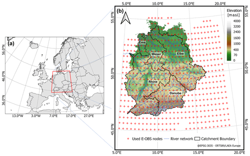
Figure 1 (a) European domain (35–70° N and 15–30° E) used for circulation pattern classification and (b) German domain (45.125–55.125° N and 5.125–19.125° E) covering the five major river basins in Germany (Danube, Elbe, Rhine, Weser, and Ems) for which the nsRWG is set up.

In this study, we apply the proposed regional WG for developing synthetic weather series for future climate scenarios. We condition the WG on CPs and regional temperature derived from an array of GCMs included in the CMIP6 (Coupled Model Intercomparison Project Phase 6) (Eyring et al., 2016). We preselected 15 CMIP6 GCMs (Table S1 in the Supplement) that have been evaluated by Cannon (2020) with regard to their ability to reproduce circulation dynamics prior to subsequent screening and weighting (Sect. 3.5).

The daily MSLP grids for the historical period (1985–2014) and two future periods spanning 2031–2060 (near future) and 2071–2100 (far future) are extracted and remapped to a consistent resolution of 1° × 1°. Further, mean daily t2m grids are extracted for the same periods, and regional daily mean temperature is computed for the German domain. We consider two shared socio-economic pathways, SSP245 and SSP585 (IPCC, 2023), for the generation of synthetic weather series. The SSP245 pathway represents a middle-of-the-road emissions trajectory marked by moderate attempts to address greenhouse gas emissions. It strives for a harmonious balance between economic growth and environmental sustainability, envisioning a world where society aims for equitable socio-economic progress while acknowledging the paramount importance of climate action. In contrast, the SSP585 pathway portrays a scenario of exceedingly high emissions with limited mitigation efforts, where economic expansion and fossil fuel usage continue to surge, casting a shadow over environmental concerns.

3 Methods

3.1 Circulation pattern classification

We employ a CP classification approach based on the SANDRA (Simulated ANnealing and Diversified RAndomization) objective classification algorithm (Philipp et al., 2007, 2016). This method is based on k-means clustering and is designed to minimize the within-cluster variance of the Euclidean distance between the cluster elements and their respective centroids. To circumvent the limitations of conventional k-means clustering, which often converges to local optima, the SANDRA algorithm introduces random reassignments of cluster elements, facilitating the search for the global optimum. Beck and Philipp (2010) and Philipp et al. (2016) found a very good performance by SANDRA compared to other classification algorithms. For use with a weather generator, it is desirable to have a CP classification, in which different CP classes have local weather characteristics that are as distinct as possible, e.g. where precipitation distributions for various CPs differ strongly. This is typically achieved with a higher number of classes (Murawski et al., 2016). However, we need to ensure that the WG has sufficient data to robustly parameterize the distributions of the weather variables for each class. With an increasing number of classes, fewer data are available within each class. Therefore, we test the SANDRA classifications with 4, 5, 6, 7, and 8 classes. To capture the seasonality in precipitation, we consider two distinct seasons for each CP: winter (November–April) and summer (May–October). Hence, in total, we test classifications with 8, 10, 12, 14, and 16 classes.

We evaluate the stratification of observed precipitation for each classification using two metrics: explained variation (EV) (Beck and Philipp, 2010) and the pseudo-F statistic (PF) (Calinski and Harabasz, 1974). EV is defined as the ratio of the sum of squared deviations from the mean within classes to the total sum of squared deviations from the overall mean. The pseudo-F statistic is the ratio of the sum of squared deviations between the class means to the mean within classes, weighted by the number of classes and cases (i.e. days). Values close to zero indicate poor stratification. EV = 1 indicates perfect stratification. Higher values for both metrics indicate better stratification.

3.2 Multi-site non-stationary weather generator

In this study, we introduce a non-stationary version of the regional weather generator (nsRWG), building upon the original stationary model developed by Hundecha et al. (2009) and further refined by Nguyen et al. (2021). Like its predecessors, the nsRWG is a multi-variate auto-regressive (MAR-1) model designed to simulate daily weather variables, including both precipitation and temperature. The non-precipitation variables are conditioned on the wet and/or dry state of the respective day according to the precipitation generated. Contrarily to the stationary versions (Nguyen et al., 2021), the precipitation generation in the nsRWG is now conditioned on CP as a latent variable characterizing changes in atmospheric dynamics. Additionally, the mean regional daily mean temperature characterizing thermodynamic changes is used as a covariate for the marginal non-stationary probability distributions.

3.2.1 Spatio-temporal dependence model

The multi-variate auto-regressive model follows Bárdossy and Plate (1992): let $W\left(t\right)=\left(W\left(t,u_{\mathrm{1}}\right),\mathrm{\dots },W\left(t,u_n\right)\right)$ be a multi-variate standard normal random vector of n locations $u=u_{\mathrm{1}},\mathrm{\dots }{u}_n$ on day t with zero mean. For the moment, we can think of W(t) as being standardized precipitation on day t. In the next step, we introduce the circulation pattern CP_i as a latent variable, where i is the circulation pattern index. We further extend the approach of Bárdossy and Plate (1992) for the estimation of the state variable by considering the transition between all pairs of circulation patterns. The MAR-1 model for the day t, which is characterized by CP_i, now reads as follows:

$$\begin{array}{}\text{(1)}& W\left(t\right)=\left\{\begin{array}{ll}{B}_{i}W\left(t-\mathrm{1}\right)+C_i\mathrm{\Psi }\left(t\right),& \text{if day }t-\mathrm{1}{\text{ has the same CP}}_i\\ {\stackrel{\mathrm{‾}}{B}}_{i}W\left(t-\mathrm{1}\right)+{\stackrel{\mathrm{‾}}{C}}_i\mathrm{\Psi }\left(t\right),& \text{if day }t-\mathrm{1}\text{ has a different CP}\\ D_i\mathrm{\Psi }\left(t\right),& \text{if }t=\mathrm{1}\text{ (starting day)}\end{array}\right.,\end{array}$$

where $\mathrm{\Psi }\left(t\right)=\left(\mathit{\psi }\left(t,u_{\mathrm{1}}\right),\mathrm{\dots },\mathit{\psi }\left(t,u_n\right)\right)$ is a random vector of the independent standard normal variable. The matrices $B_i{\stackrel{\mathrm{‾}}{B}}_i{C}_i$, ${\stackrel{\mathrm{‾}}{C}}_i$, and D_i are related to the lag-0 correlation matrix (M_i0), the lag-1 correlation matrix (M_i1) within a single CP_i, and the lag-1 correlation matrix (${\stackrel{\mathrm{‾}}{M}}_{i\mathrm{1}})$ for the transition between CP_s values other than CP_i to CP_i.

$$\begin{array}{}\text{(2)}& {\displaystyle }{B}_i=M_{i\mathrm{1}}{M}_{i\mathrm{0}}^{-\mathrm{1}}\text{(3)}& {\displaystyle }{\stackrel{\mathrm{‾}}{B}}_i={\stackrel{\mathrm{‾}}{M}}_{i\mathrm{1}}{M}_{i\mathrm{0}}^{-\mathrm{1}}\text{(4)}& {\displaystyle }{C}_i{C}_i^T=M_{i\mathrm{0}}-B_i{M}_{i\mathrm{1}}^T\text{(5)}& {\displaystyle }{\stackrel{\mathrm{‾}}{C}}_i{\stackrel{\mathrm{‾}}{C}}_i^T=M_{i\mathrm{0}}-{\stackrel{\mathrm{‾}}{B}}_i{\stackrel{\mathrm{‾}}{M}}_{i\mathrm{1}}^T\text{(6)}& {\displaystyle }{D}_i{D}_i^T=M_{i\mathrm{0}}\end{array}$$

In the above, the superscripts −1 and T indicate the matrix inversion and matrix transpose operator, respectively.

The introduction of ${\stackrel{\mathrm{‾}}{M}}_{i\mathrm{1}}$,${\stackrel{\mathrm{‾}}{B}}_i$ and ${\stackrel{\mathrm{‾}}{C}}_i$ represents an enhancement compared to the previous works by Bárdossy and Plate (1992), Hundecha et al. (2009), and Nguyen et al. (2021) when dealing with frequently alternating CPs. Previous studies re-initialized the precipitation state every time there was a shift in a latent variable state, i.e. a shift in CP (Bárdossy and Plate, 1992) or a change between months (Hundecha et al., 2009; Nguyen et al., 2021).

We estimate the correlation matrices (M_i0, M_i1, and ${\stackrel{\mathrm{‾}}{M}}_{i\mathrm{1}}$) through the Kendall correlation and then transform them into a Pearson's correlation (Serinaldi and Kilsby, 2014; Nguyen et al., 2021). To correct for poorly defined (not positive-definite) lag-0 correlation matrices M_i0, we use the method of Higham (2002) to find the nearest positive-definite correlation.

3.2.2 Marginal distributions

We use the three-parameter extended generalized Pareto distribution (Naveau et al., 2016; Nguyen et al., 2021) to model the non-zero daily precipitation distribution at every location u for each CP, i.e. the marginal distribution. The cumulative probability distribution function for non-zero precipitation x is given by

$$\begin{array}{}\text{(7)}& F\left(x(t,u)\right)=\left\{\begin{array}{ll}{\left(\mathrm{1}-{\left(\mathrm{1}+\mathit{\sigma }{\left(t,u\right)}^{-\mathrm{1}}\mathit{\xi }x(t,u)\right)}^{-{\mathit{\xi }}^{-\mathrm{1}}}\right)}^k& \text{for }\mathit{\xi }>\mathrm{0}\\ \left(\mathrm{1}-\exp \left(-\mathit{\sigma }{\left(t,u\right)}^{-\mathrm{1}}x(t,u)\right)\right){}^k& \text{for }\mathit{\xi }=\mathrm{0}\end{array}\right.,\end{array}$$

where κ controls the shape of the lower tail, σ is a scale parameter, and ξ>0 controls the decay rate of the upper tail. The scale parameter σ is allowed to covary with the regional daily mean temperature (Eq. 8). The exponential function is used to ensure that the scale parameter is positive:

$$\begin{array}{}\text{(8)}& \mathit{\sigma }\left(t,u\right)=\exp \left({\mathit{\sigma }}_{\mathrm{0}}\left(u\right)+\text{t2m}\left(t\right)\cdot {\mathit{\sigma }}_{\mathrm{1}}\left(u\right)\right).\end{array}$$

We employ the Shuffled Complex Evolution–University of Arizona (SCE-UA) global optimization algorithm (Duan et al., 1992) to estimate the parameters κ, ξ, σ₀, and σ₁ by optimizing the log-likelihood function.

The complete precipitation process including wet and dry conditions with non-negative precipitation x for a certain CP at an individual location u is modelled using the cumulative distribution H(x):

$$\begin{array}{}\text{(9)}& H\left(x\left(t,u\right)\right)=\left\{\begin{array}{ll}\left(\mathrm{1}-p\left(u\right)\right)+p\left(u\right)\cdot F\left(x\left(t,u\right)\right),& x\left(t,u\right)>\mathrm{0}\\ \mathrm{1}-p\left(u\right),& x\left(t,u\right)=\mathrm{0}\end{array}\right.,\end{array}$$

where p represents the wet frequency, and (1−p) stands for the probability of zero rainfall. The link between the marginal distribution of precipitation (Eq. 9) and the MAR-1 model (Eq. 1) is given by

$$\begin{array}{}\text{(10)}& \mathrm{\Phi }\left(W\left(t,u\right)\right)=H\left(x\left(t,u\right)\right),\end{array}$$

where Φ stands for the cumulative distribution function of a standard normal distribution.

For simulating daily average temperature fields consistent with non-stationary precipitation fields, we condition marginal temperature distributions for each month on the wet and/or dry state of precipitation. Similarly to Nguyen et al. (2021), we apply a normal distribution to model daily temperature data. To accommodate the non-stationary change due to increasing regional temperature, we use it as a covariate for the location parameter of the non-stationary normal distribution:

$$\begin{array}{}\text{(11)}& \mathit{\mu }\left(t,u\right)={\mathit{\mu }}_{\mathrm{0}}\left(u\right)+{\mathit{\mu }}_{\mathrm{1}}\left(u\right)\cdot \text{t2m}\left(t\right),\end{array}$$

where μ is the location parameter of the normal distribution, and parameters μ₀ and μ₁ are estimated by optimizing the log-likelihood function analogously to the parameters of the marginal precipitation distribution. Finally, temperature fields are also simulated using a multi-variate MAR-1 model analogously to precipitation.

3.3 Model setup and performance evaluation

The nsRWG is set up for the study area using the observed gridded dataset E-OBS v25.0e. The model is calibrated for 540 grid cells. For each combination of CP and season (winter or summer), 100 realizations are generated with a time series length of 72 years, the same length as for the observed data. Synthetic and observed climates are compared using several statistical metrics introduced below. This evaluation procedure is commonly applied to assess stochastic weather models (Kleiber et al., 2012; Breinl et al., 2013; Serinaldi and Kilsby, 2014; Baxevani and Lennartsson, 2015; Nguyen et al., 2021).

In the evaluation process, special attention is given to both the local and spatial model performance. For the local evaluation, the following at-site metrics are computed and compared with observations:

• Precipitation intermittence properties. This includes wet-day frequency and four transition probabilities (wet-to-wet, wet-to-dry, dry-to-wet, and dry-to-dry). We consider days to be dry if the recorded daily precipitation is below 0.1 mm.

• Daily precipitation for each CP. This includes the mean and 99.5th percentile.

• Seasonal precipitation total for each CP. This includes the mean and 98th percentile.

Both the 99.5th and 98th percentiles are estimated using the semi-parametric quantile estimation proposed by Hutson (2002).

• n d maxima. The total precipitation for n=5 and 10 d is compared to the observed statistics to analyse the plausibility of wet-spell precipitation amounts. We consider these durations to be important for the generation of flood events by single cyclones and for flood events resulting from subsequent storms, with the preceding storms contributing to the catchment wetness.

The ability of the nsRWG to reproduce daily average temperature is assessed for each month by comparing the observed mean and 99.5th percentile values from the observation period to the simulated values.

To evaluate the spatial representation of precipitation fields, for each circulation pattern and season, we examine the following:

• The correlation of precipitation as a function of distance between pairs of locations. This includes lag-0 (M₀), lag-1 (M₁) for the transition between days with the same CP, and lag-1 (${\stackrel{\mathrm{‾}}{M}}_{\mathrm{1}}$) for the transition between days characterized by different CPs.

• The catchment areal precipitation. This includes the 99.5th percentile of catchment average precipitation for the five major river basins in Germany.

For a consistent and comparable assessment of model performance, we adopt the evaluation and performance framework (CASE) for weather generators proposed by Bennett et al. (2018). In the first step, the at-site performance is assessed for each at-site metric. The performance is categorized as “good” (G), “fair” (F), or “poor” (P) at each location, i.e. grid cell. Model performance is considered to be good if the observed metric falls within the 90 % range of the metric values computed for 100 model realizations. Fair performance is assigned when the observations are outside the 90 % range but within the 99.7 % limits or if the absolute relative difference (RD) between the observed and simulated metric means is 5 % or less. Poor performance is indicated when neither of these conditions is met. RD is defined as follows:

$$\begin{array}{}\text{(12)}& \text{RD}=\left|{\displaystyle \frac{M_{\mathrm{obs}}-{\stackrel{\mathrm{‾}}{M}}_{\mathrm{sim}}}{M_{\mathrm{obs}}}}\times \mathrm{100}\right|,\end{array}$$

where M_obs is the metric value based on observations, and ${\stackrel{\mathrm{‾}}{M}}_{\mathrm{sim}}$ is the mean metric value based on simulated data.

The overall performance is assessed by computing the share of sites exhibiting good, fair, and poor performance. Overall performance is classified into six categories (Bennett et al., 2018):

• “overall good” if more than half of the locations show good performance

• “overall fair” if more than half of the locations show fair performance

• “overall poor” if more than half of the locations show poor performance

• “overall fair–good” if the total percentage of fair- and good-performance locations exceeds the percentage of locations with poor performance

• “overall fair–poor” if the total percentage of fair- and poor-performance locations exceeds the percentage of locations with good performance

• “overall variable” if the total percentage of good- and poor-performance locations exceeds the percentage of locations with fair performance.

3.4 Downscaling future precipitation

To showcase the practical value of the newly developed weather generator, we employ it to downscale precipitation for future climate projections from nine global climate models. The GCMs are selected from the list of models in Table S1 using a mixture of qualitative and quantitative considerations regarding their performance in simulating European climate and taking into account their independence. The selection is carried out to reduce the computational load for the nsRWG and subsequent future climate impact studies on flood risk change. The main guide for the selection is the model performance weights calculated using the ClimWIP (Climate model Weighting by Independence and Performance) method (Brunner et al., 2020) as implemented in the ESMValTool (Earth System Model Evaluation Tool) version v2.6.0 (Eyring et al., 2020; https://docs.esmvaltool.org/en/latest/recipes/recipe_climwip.html, last access: 1 June 2023). As performance metrics, we use the models' distances to ERA5 in the European domain for the 1985–2014 climatology and the annual variability of temperature and sea level pressure, as well as the temperature trend. This follows the metric selection of Brunner et al. (2020) but targeting Europe. We also ensure that the final selection of models follows the recommendations for model selection from the recent work by Merrifield et al. (2023), who considered model performance, independence, and spread as criteria. The resulting ClimWIP performance weights are summarized in Fig. 2.

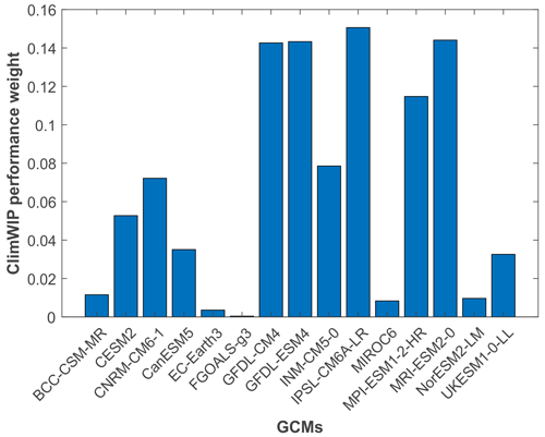
Figure 2 Performance weights for 15 GCMs (Table S1) resulting from the ClimWIP procedure based on the preselected evaluation criteria for the historical period 1985–2014.

Based on the resulting weights, we select nine models to be used in this study. The only exceptions are the two GFDL models, from which we select only the (better-performing) Earth system version even though they both received high weights. This is done to limit the inter-dependency in our model pool. Our selection includes UKESM1-0-LL, CanESM5, CESM2, CNRM-CM6-1, INM-CM5-0, MPI-ESM1-2-HR, MRI-ESM2-0, GFDL-ESM4, and IPSL-CM6A-LR. For these models, the independence weights are also computed and can be used in future climate impact studies.

Overall, we investigate 36 distinct cases, which result from the combination of nine GCM models, two pathways, and two future periods. To this end, for each of these cases, we generate 100 realizations of daily time series with the nsRWG conditioned on the respective CPs and regional daily mean temperature corrected for bias with respect to ERA5 using quantile mapping (R package qmap by Gudmundsson et al., 2012).

4 Results and discussion

4.1 Circulation pattern classification and mean regional temperature

The results of the classification of circulation patterns indicate relatively low values of EV below 0.1 and of log(PF) between 2 and 2.3, showing a similar range as in Murawski et al. (2016). The differences between classifications with different numbers of classes (between four and eight) are relatively small, especially for cases with more than six classes. Therefore, we adopt the final classification with six CPs and consider this to be a good compromise between the degree of stratification (i.e. EV and PF) and the data available to estimate the marginal distributions. In total, the entire period is stratified into 12 classes (i.e. six CPs and two seasons), which is similar to a classical monthly based parameterization used by Hundecha and Merz (2012) and Nguyen et al. (2021), with the difference being that days are unevenly distributed between classes. We also compare the EV and PF metrics and examine the stratified precipitation patterns between the CP-based classifications and the monthly based classification calculated for the current precipitation dataset (not shown). The CP-based classification with more spatially distinct stratification shows somewhat better performance than the monthly based classification, although the overall values of EV and PF are low. This suggests that, while both approaches exhibit low explanatory power for precipitation, CP-based classification provides a more useful framework for capturing variability compared to the classical monthly based approach. Moreover, using CP-based stratification may allow us to assess the impact of potential changes in CP frequency and persistence in future climate projections.

Figure 3 shows the mean sea level pressure (MSLP) of the six patterns of the selected classification. CP2 and CP4 are characterized by high-pressure systems covering a large region, particularly around central Europe. The descending air associated with these high-pressure systems inhibits cloud formation and precipitation, leading to stable and dry weather conditions, often characterized by sunny days. CP3 includes the days with weak pressure gradients and is associated with moderate precipitation and weather conditions. CP1, CP5, and CP6 exhibit distinct low-pressure systems over large areas. As a result, these regions are prone to cloudy and wet weather conditions. CP5, in particular, shows an extremely low-pressure area in the North Atlantic region, creating a steep positive pressure gradient towards central Europe. The steep pressure gradient can drive strong winds and lead to intense precipitation events in central Europe. The winter, summer, and annual frequencies of the CPs are summarized in Table 1. In winter, CP3 is the most frequent, with 36.8 %, while CP5 is the rarest, with only 3.8 %. In summer, CP2 takes the lead with 19.6 %, and CP4 and CP6 are close behind with 17.0 % each. For the whole year, CP3 is the most frequent, with 26.3 %, followed by CP1, with 17.3 %. CP5 is again the least frequent, with 10.2 %. These numbers give an idea of how different CPs play out over the seasons.

Table 1 Winter, summer, and annual frequencies of the selected classification with six CPs.

The regional average daily temperature over the period 1950–2021 shows a mean of 8.6 °C and a standard deviation of 7.3 °C. In this period, a significant positive trend of 0.27° per decade (p value <0.01) is detected based on the E-OBS data. The overall change in regional average annual temperature amounts to 1.9 °C from 1950. The pronounced increase in temperature underscores the potential relevance of thermodynamic changes in the atmosphere to be considered in the nsRWG parameterization.

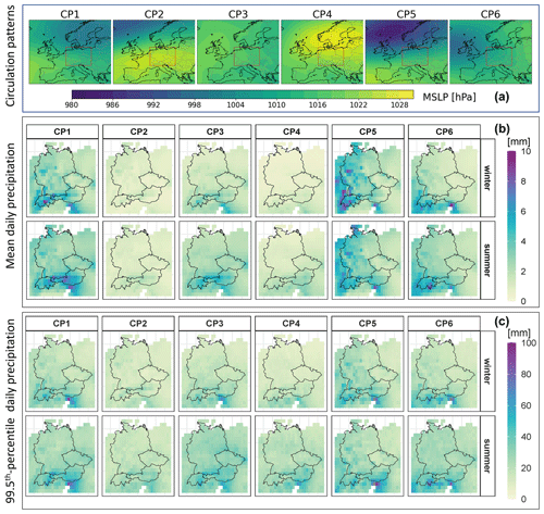
Figure 3 (a) Selected circulation pattern classification with six patterns. The maps show the average mean sea level pressure of all the days falling into the same pattern. The red box in the maps shows the German domain. (b) Mean daily precipitation observed for the six CPs during winter and summer seasons and (c) 99.5th percentile daily precipitation observed for six CPs during winter and summer seasons.

Figure 3 illustrates the stratification of daily precipitation intensity, examining the mean and 99.5th percentile of the classification based on the six CPs further divided into summer and winter. We observe a clear distinction between CPs in terms of mean and extreme precipitation. CP2 and CP4 stand out as rather dry patterns, on average, whereas CP5 and CP1 are relatively wet in both seasons. CP3 and CP6 show average wetness which varies slightly between seasons. CP1 and CP5 exhibit high extreme precipitation in both seasons. Additionally, CP3 and CP6 bring about extreme rainfall in the summer season throughout the German domain.

4.2 Marginal distribution fitting

We model the marginal precipitation distributions with the extended generalized Pareto distribution (extGPD) based on precipitation data stratified into 12 classes according to CPs and seasons. We assess the model fitting for both stationary and non-stationary model versions (see Sect. 3.2.2), where the former is indeed a nested form of the latter. The goodness of fit of the stationary model was evaluated using the Kolmogorov–Smirnov (KS) test, the Cramér–von Mises (CVM) test, and the Anderson–Darling test, which indicated that the stationary model adequately fits the observed data at a significance level of 0.05 (results not shown). However, applying traditional goodness-of-fit tests in a non-stationary context is challenging as these tests must be performed at each time step due to time-varying parameters. Therefore, we employ the corrected Akaike information criterion (AICc) (Akaike, 1973; Burnham and Anderson, 2004) to measure the relative quality of the two models in fitting the data, as recommended in several studies (Cannon, 2010; Villarini et al., 2009; Kim et al., 2017). AICc, like other information criteria, does not provide direct measures of goodness of fit. However, it reflects how well the model fits the data through the likelihood function while penalizing for the number of parameters (model complexity). Consequently, a model with a lower AICc should be preferred in the model selection process (Burnham and Anderson, 2004).

To compare the performance of the two distribution models in fitting data across all locations for CP and season, we calculate the percentage of locations where the non-stationary model shows a lower AICc value compared to the stationary model and vice versa. This analysis allows us to derive a measure called the difference in model performance, where a positive value indicates a preference for the non-stationary model. Figure 4 illustrates that the non-stationary model provides a better fit for more than 50 % of the cells for CP1, CP3, CP4, and CP6 in both seasons; for CP1, CP3, and CP4, this is even in over 75 % of the cells. For CP2, characterized by rather dry conditions, the non-stationary model is better for about 70 % of the cells in summer. In winter, the stationary model has a slight edge. For CP5 (wet conditions), the non-stationary model has a slight advantage in winter, but only 25 % of the cells are better simulated in summer. Overall, the non-stationary model is preferred over its nested version in approximately 70.5 % of fitting cases. This supports our decision to utilize the non-stationary model for fitting marginal distributions in subsequent analyses.

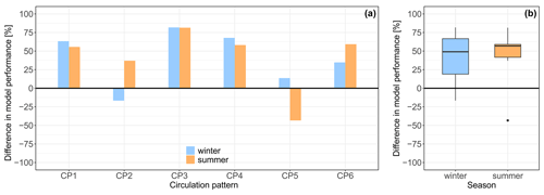
Figure 4 Difference in model performance in terms of fitting marginal distributions of extGPD to precipitation data between the non-stationary and stationary models for six CPs and two seasons (a) and summarized for two seasons (b). A positive value indicates better performance for the non-stationary case.

4.3 Evaluation of the nsRWG performance

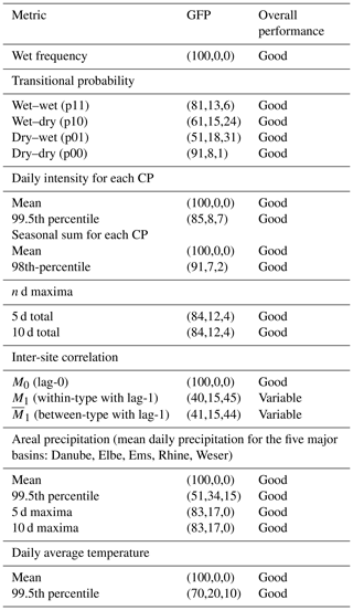
The at-site and spatial performance of the nsRWG is evaluated using the performance metrics described in Sect. 3.4. We use the good, fair, poor (GFP) score, which indicates the percentage of locations that have good, fair, and poor performance with respect to each metric considering all 100 realizations. Table 2 summarizes the performance statistics, which are discussed in detail in the following sections. Although a direct comparison with the performance of the stationary RWG model of Nguyen et al. (2021) is not straightforward due to the different underlying datasets (gridded E-OBS vs. station-based), we discuss the nsRWG performance in the context of the stationary model evaluation.

Table 2 Summary of the model performance statistics for the nsRWG and categorization of the model performance according to Bennett et al. (2018).

4.3.1 At-site nsRWG performance

The nsRWG replicates the essential statistic of the observed wet-day frequency (Fig. 5, top row) with a perfect GFP score (100,0,0) across the model domain. This consistent performance is evident in both seasons, as shown by the red dots closely aligned with the 1:1 line. The narrow grey bars reflect small uncertainty. CP1, CP5, and CP6 display a higher number of wet days compared to CP2, CP3, and CP4, consistently with our inference from the circulation patterns in Sect. 4.1 (Figs. 2 and 3).

The nsRWG reproduces the four transition probabilities reasonably well (Table 2). The model is particularly good at capturing the wet-to-wet (p11) and dry-to-dry (p00) transitions. Wet-to-dry (p10) and dry-to-wet (p01) transitions are more challenging, but the overall performance is still categorized as good. The performance across the CPs and seasons is nearly uniform, with some small variations (Fig. 5). For instance, the transition probabilities in dry-to-wet transitions are slightly overestimated for CP1, CP3, and CP4 in both seasons. CP5 generally shows larger variability in performance across model realizations. The nsRWG performance with regard to wet-day frequency and transition probabilities is comparable to the stationary model performance (Nguyen et al., 2021).

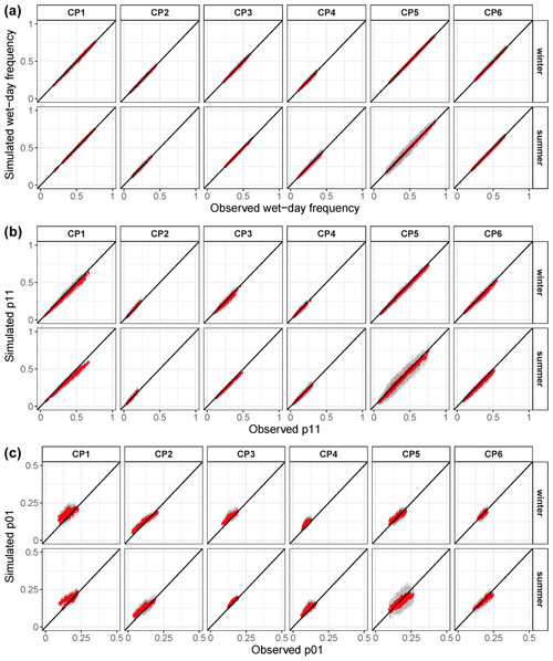
Figure 5 Comparison of observed and simulated wet-day frequency (a) and transition probabilities (p11: wet-to-wet; p01: dry-to-wet) of daily precipitation (b, c) in all grid cells. Red dots represent the median of the grey range corresponding to 100 model realizations.

The nsRWG accurately reproduces mean daily precipitation sums and the 99.5th percentile of daily precipitation (Table 2). The performance for extreme precipitation is fairly uniform across CPs and seasons (Fig. 6); i.e. most of the red dots are close to the 1:1 line.

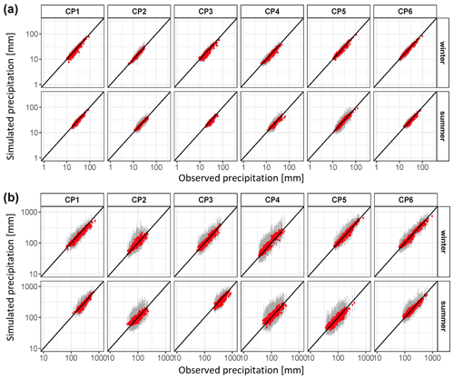
Figure 6 Comparison of observed and simulated extreme (99.5th percentile) daily precipitation (a) and 98th percentile seasonal precipitation total (b) for each CP in all grid cells. Red dots represent the median of the grey range corresponding to 100 model realizations.

The nsRWG performance with regard to the seasonal precipitation sum for each CP is good (Table 2). The mean of the seasonal sum is perfectly matched (Table 2), but the 98th percentile is also reproduced very well for all CPs (Table 2, Fig. 6). Dry CPs (CP2 and CP4) show quite a strong variability in the 98th percentile of seasonal precipitation sums in comparison to wetter CPs. In summer, CP5 also exhibits strong variability between different model realizations (Fig. 6). Though this pattern is associated with high mean and extreme daily precipitation (Fig. 3), the total seasonal precipitation sum is relatively small (Fig. 6). For all CPs and seasons, the median of model realizations is close to the 1:1 line, which is what should be expected for a good model performance.

Figure 7 shows the good performance of the nsRWG in reproducing 5 and 10 d precipitation annual maxima. This statistic reflects the model's ability to correctly generate maximum multi-day precipitation, which is particularly relevant for flooding. This metric integrates the model performance with respect to auto-correlation, transition probabilities, and marginal probabilities. Although autocorrelation and transition probabilities are generally linked to averages, their influence can also extend to extremes, particularly in capturing variability in multi-day events. The overall performance (Table 2) is good and shows notable improvement compared to the stationary model application (Nguyen et al., 2021). Additionally, we compared frequency plots for observed and simulated multi-day precipitation in nine exemplary grid points across the domain (Fig. S1). The range of simulated precipitation quantiles encompasses the observed quantiles well across the entire empirical probability range.

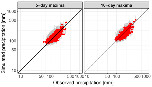
Figure 7 Comparison of observed and simulated multi-day precipitation sums accumulated over 5 and 10 d periods in all grid cells. Red dots represent the median of the grey range corresponding to 100 model realizations.

The nsRWG excels in reproducing the mean of daily average temperature in each month at all locations (Table 2). The performance with regard to the 99.5th percentile of daily average temperature is slightly weaker but still good overall (Table 2). It is obviously more challenging for the nsRWG to match the extreme percentiles compared to the mean. The performance with regard to the 99.5 percentile is fairly stable across all months (Fig. 8), and most of the red dots corresponding to the mean of 100 realizations align closely to the 1:1 line. The spread in the winter half-year (November–March) is, however, slightly stronger than in the summer half-year (May–October). The performance of the non-stationary model version is comparable to or even slightly better than that of the stationary RWG (Nguyen et al., 2021). To compare the dependency between the extreme daily temperature and precipitation states, we additionally explore the observed and simulated difference in dry-day and wet-day extreme temperatures across the year (Fig. S2). The satisfactory results demonstrate the expected dependency between precipitation state and extreme temperature.

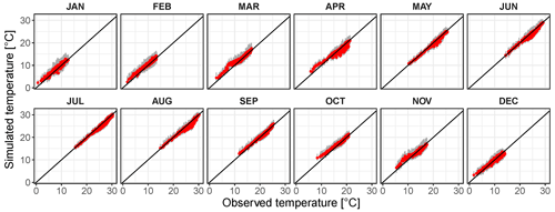
Figure 8 Comparison of observed and simulated 99.5th percentile average daily temperature for all months and grid cells. Red dots represent the median of the grey range corresponding to 100 model realizations.

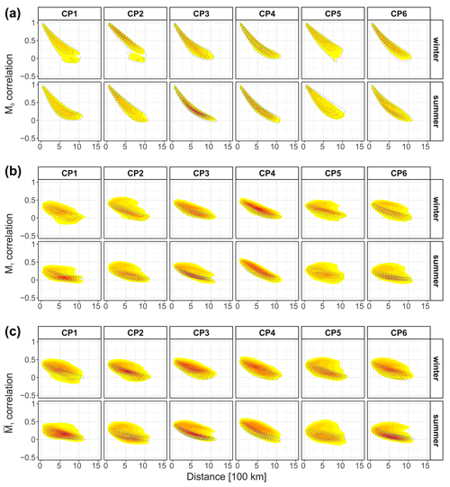
Figure 9 Comparison of observed and simulated spatial correlation versus inter-site distance: M₀ lag-0 correlation (a), M₁ within-type correlation (b), and ${\stackrel{\mathrm{‾}}{M}}_{\mathrm{1}}$ between-type correlation (c). Increasing density of points for the observed series is indicated in shaded colours from yellow to red. The density of points for the simulated series is indicated by the contour lines.

4.3.2 Spatial nsRWG performance

Figure 9 provides an overview of the nsRWG's ability to replicate the spatial dependence structure, as characterized by three different types of correlation: M₀ (lag-0), M₁ (within-type with lag-1), and ${\stackrel{\mathrm{‾}}{M}}_{\mathrm{1}}$ (between-type with lag-1). The simulated M₀ correlation closely aligns with the observed correlation structure, demonstrating a close match even for inter-site distances of up to 1100 km. However, the other two correlation types, M₁ and ${\stackrel{\mathrm{‾}}{M}}_{\mathrm{1}}$, are partly significantly underestimated across all CPs and seasons. This is particularly evident in the case of ${\stackrel{\mathrm{‾}}{M}}_{\mathrm{1}}$; i.e. the model has some difficulties in representing spatial rainfall during transitions between days characterized by two different CPs. Exploring the incorporation of orographic effects or anisotropy (e.g. Liu et al., 2024) into the representation of the spatial dependence structure of the nsRWG could be beneficial for future work.

Despite some deficiencies in reproducing the spatial correlation, the nsRWG is capable of reproducing various characteristics of the catchment average precipitation (mean, 99.5th percentile, 5 and 10 d annual maxima) for the five major river basins in Germany (Table 2). The performance in terms of areal extreme (99.5th percentile) daily precipitation is fairly good and consistent across all basins and CPs (Fig. 10). The model underestimates the extreme areal precipitation slightly, particularly in summer, which is the consequence of the underestimation of spatial correlations (Fig. 9).

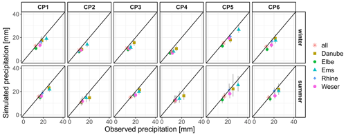
Figure 10 Comparison of observed and simulated extreme (99.5th percentile) daily precipitation averaged over the five major river basins in Germany (Danube, Elbe, Ems, Rhine, and Weser) and over the whole domain (all). The coloured dots represent the median of the grey range corresponding to 100 realizations.

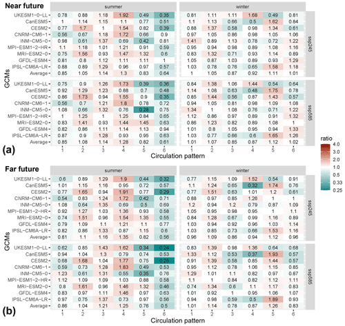
Figure 11 Changes in projected circulation pattern frequency for the near future (a) and the far future (b). The changes in frequency are represented by the ratio between CP frequency in the future and the control periods. “Average” represents the average frequency changes across the nine selected GCMs.

4.4 Future projected changes

In the following section, we demonstrate an application of the nsRWG for the generation of long synthetic precipitation series conditioned on the selected CMIP6 GCMs in historical and near- and far-future periods. To this end, we consider the topology of individual CPs (Fig. 3, top row) derived for the past period to remain stable in future. Thus, only the frequency and persistence of CPs change with time. Furthermore, the spatio-temporal structure of precipitation is considered to be stationary. Another fundamental assumption of the presented approach is that the climate for each of the 30-year periods is regarded to be stationary. The non-stationarity of CPs and of the regional temperature within these periods prescribes the variability of long-term synthetic weather generated by the nsRWG. The non-stationarity of climate between the 30-year periods can be considered by means of changes in CPs and regional temperature over time. Here, the aim is not to provide a detailed analysis of projected changes in dynamics and thermodynamics but rather to demonstrate how these explain changes in statistically downscaled extreme precipitation over Germany. A more comprehensive analysis of projected changes in the atmosphere and the associated flood hazard and risk is the focus of future research.

4.4.1 Changes in circulation pattern frequency and persistence

Projected changes in the frequency of CPs are more pronounced in summer than in winter across all GCMs (Fig. 11). The nine selected GCMs are mostly consistent in projecting the frequency changes of the six CPs in summer but show a more mixed pattern in winter. This behaviour is similar in both the near- and far-future periods and for both SSPs. In summer, wetter CPs such as CP1, CP5, and CP6 become less frequent in nearly all GCMs. In particular, the reduction in the frequency of CP6 is pronounced and consistent in all but one GCM. On the contrary, drier patterns (CP2 and CP4) and the average wet pattern of CP3 become more frequent in summer. The driest, CP4, experiences the strongest positive change. The UKESM1-0-LL model projects that the frequencies of this pattern almost double in the near future. In winter, changes are less consistent across models and periods. On average, a slight increase is projected for the wetter CP5 characterized by westerly flows and responsible for extreme precipitation, particularly in western and southwestern Germany (Fig. 3). The drier winter patterns, CP3 and CP4, show a slight reduction in the occurrence frequency (factors between 0.78 and 0.94, on average), which is mostly consistent across GCMs. Here, UKESM1-0-LL stands out and shows an opposite tendency (Fig. 11).

4.4.2 Changes in regional temperature

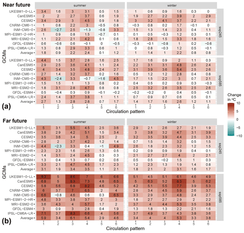
Changes in mean regional temperature corrected for bias between the historical and control periods are analysed across SSPs, GCMs, CPs, and seasons (Fig. 12). Since the marginal precipitation distributions are conditioned on the regional temperature for each CP, this is a valuable insight into how temperature changes for different CPs. The vast majority of GCMs indicate a positive regional temperature change for future periods. Only a few GCMs (e.g. INM-CM5-0 and GFDL-ESM4) show negative changes for some CPs. The far future and the more pessimistic SSP585 scenario show stronger positive changes, as expected. The positive signals are stronger in summer than in winter. The temperature change is weakest for the wettest pattern, CP5, in all models and scenarios. One of the driest patterns, CP4, shows the strongest temperature increase in both summer and winter. Circulation patterns CP1 and CP3, which are medium wet patterns concerning both average and extreme precipitation (Fig. 3), show a relatively strong positive temperature change. While the CP1 frequency is consistently decreasing (Fig. 11), the projected frequency of CP3, in combination with positive temperature, will increase the importance of CP3 for total precipitation input in the future. The average summer and winter temperature changes for the far future and the SSP585 scenario are in the range of changes assessed by Coppola et al. (2021a) for a somewhat larger CMIP6 GCM ensemble in the central European region.

Figure 12 Changes in average regional temperature between the historical scenario and the near future (a) and the far future (b) across nine GCM projections, two SSPs, six CPs, and two seasons. “Average” represents the average change across the nine selected GCMs.

4.4.3 Changes in future extreme precipitation generated with the nsRWG

Here, we present the changes in extreme precipitation conditioned on future climate projections. We examine the plausibility of seasonal and spatial patterns of changes in extreme precipitation in relation to the available literature. This discussion is impaired by the still-small number of CMIP6-based analyses of extreme precipitation over the central European domain. An in-depth analysis of downscaled precipitation data and a comprehensive flood impact assessment will be addressed in a separate, forthcoming study.

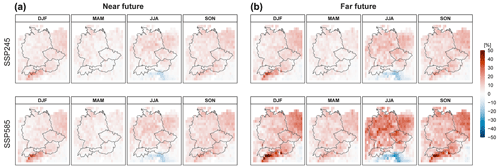
Figure 13 Changes in extreme (99.5th percentile) daily precipitation between the historical and the near-future periods (a) and the historical and far-future periods (b) for winter (DJF), spring (MAM), summer (JJA), and autumn (SON) and for two SSP scenarios. The results are averaged over nine GCM models and 100 nsRWG realizations.

Extreme daily precipitation from the nsRWG is projected to consistently increase over the target region, except over northern Italy, in the summer months (JJA) (Fig. 13). The overall increase in extreme precipitation is in line with the assessment of the CMIP6 GCM ensembles for western and central Europe for the 99th percentile daily precipitation (Coppola et al., 2021a, b) and for the seasonal 20-year return period precipitation (Ritzhaupt and Maraun, 2023), although the model spread is considerable, particularly in summer. Decreases in summer over Italy for daily mean and hourly extreme precipitation are consistent with the MPI-ESL-LL downscaled by the WRF regional climate model driven by the CMIP5 RCP4.5 scenario (Knist et al., 2020). According to the nsRWG, the precipitation increase for SSP245 is mostly in the range of up to 20 % and up to 40 % in the near and far future, respectively, for all seasons (Fig. 13). The increase is stronger for SSP585 compared to SSP245 and is particularly pronounced in the summer months (JJA) in the far future. However, the autumn months (SON) also show a notable increase. Given the decreasing frequency of the wetter CPs in the summer half-year, the increase in extreme precipitation is likely to be dominated by thermodynamic changes. However, the question of attributing precipitation and flood changes to changes in the dynamic and thermodynamic components is the subject of future research.

5 Conclusions

In this paper, we develop a non-stationary version of the auto-regressive regional weather generator (nsRWG) conditioned on circulation patterns (CPs) and regional daily mean temperature. The nsRWG is designed to generate a synthetic long-term (thousands of years) daily weather series for use with hydrological impact models to assess future flood risks. By conditioning the nsRWG on CPs and regional temperature, we consider the effect of changes in the dynamic and thermodynamic properties of the atmosphere on changes in local precipitation. The non-stationary extended generalized Pareto distribution is used to simulate the marginal precipitation distributions. CPs are used as a latent variable to parameterize the marginal non-stationary precipitation distributions, whose scale parameter is conditioned on the regional daily mean temperature. Temperature data are modelled using a non-stationary normal distribution conditioned on the regional daily mean temperature.

The nsRWG is set up for a domain of more than 650 000 km² covering five major river basins in Germany – the Danube, Elbe, Rhine, Weser, and Ems – using E-OBS gridded observation data of daily precipitation and temperature. Circulation patterns and the regional temperature are derived based on the ERA5 reanalysis. The evaluation of the nsRWG following the CASE framework by Bennet et al. (2018) shows overall good results with regard to the at-site precipitation intermittency properties, i.e. the mean and extreme (99.5th percentile) daily and multi-day precipitation sums. The comparison with a stationary precipitation model version, which does not include temperature as a covariate in the marginal precipitation distributions, shows a superior performance compared to the non-stationary model for more than 70 % of grid cells in the study area. Matching the spatial correlation structure of precipitation remains a challenge for the nsRWG, particularly when transitioning between days with different CPs. Nevertheless, the areal extreme precipitation for the major German river basin is very well reproduced by the model. The nsRWG excels in simulating a minimum, mean, and maximum daily temperature and their extreme percentiles.

The link between large-scale atmospheric characteristics such as CPs and regional temperature on one side and local precipitation and temperature on the other allows us to use pressure and temperature variables from the general circulation models (GCMs) to generate local weather and, at the same time, to account for the climate change signal manifested in changes in the frequency and persistence of circulation patterns and regional warming. This approach is charming as it relies on the mean sea level pressure for CP classification and on the regional temperature – two variables that are simulated by the global climate models more skilfully than precipitation. We demonstrate the application of the nsRWG for downscaling the precipitation from nine CMIP6 GCMs weighted by the ClimWIP approach. The latter is used to assess the skill of GCMs in reproducing the mean, variability, and trend of the covariates (mean sea level pressure and regional temperature) in the historical period (1985–2014). The results suggest a consistent increase in extreme precipitation over the German basins in the near (2031–2060) and far (2071–2100) future, in line with the previous regional analyses of various CMIP6 ensembles. By generating a long synthetic series for each of the historical and future periods, we can estimate precipitation change more robustly than if we were only using a 30-year series directly available from a climate model. Hence, the nsRWG offers a key benefit for hydrological impact studies by providing long-term (thousands of years) consistent synthetic weather data indispensable for the robust estimation of high flood flow quantiles and future flood risk changes.