Reducing reliability bias in assessments of extreme weather risk using calibrating priors

A number of recent climate studies have used univariate parametric statistical models to estimate return periods of extreme weather events based on the method of maximum likelihood. Using simulations over multiple training datasets, we find that using maximum likelihood gives predictions of extreme return levels that are exceeded more often than expected. For instance, when using the generalised extreme value distribution (GEVD) with 50 annual data values, fitted using maximum likelihood, we find that 200-year return levels are exceeded more than twice as often as expected; i.e. they are exceeded in more than 1 in 100 simulated years. This bias, which we refer to as a predictive coverage probability (PCP) bias, would be expected to lead to unreliable predictions. We review the theory related to Bayesian prediction using right Haar priors which gives an objective way to incorporate parameter uncertainty into predictions for some statistical models and which eliminates the bias. We consider a number of commonly used parametric statistical models and give the right Haar priors in each case. Where possible, we give analytical solutions for the resulting predictions. Where analytical solutions are not possible, we apply either an asymptotic approximation for the Bayesian prediction integral or ratio of uniforms sampling. For the fully parameterised GEVD and the generalised Pareto distribution with a known location parameter, neither of which have a right Haar prior, we test a number of methods and find one that gives big reductions in the PCP bias relative to maximum likelihood predictions. Finally, we revisit the De Bilt extreme temperature example considered in a number of previous studies and generate revised, and shorter, estimates for the return period of the 2018 heatwave. Software for fitting predictive distributions with parameter uncertainty has been developed by the first author and will be available as an R package.

1 Introduction

A number of recent studies in the field of extreme weather attribution have estimated the return probabilities and return levels of extreme weather events, in past, present, and possible future climates. See, for example, Philip et al. (2022), Otto et al. (2023), Rivera et al. (2023), Thompson et al. (2023), Vautard et al. (2023), and Zachariah et al. (2023). Overviews of some of the methodologies used in extreme weather attribution are given in Philip et al. (2020), van Oldenborgh et al. (2021), and van Oldenborgh et al. (2022), and aspects of the uncertainty in extreme weather attribution have been discussed in Jeon et al. (2016) and Paciorek et al. (2018).

1.1 Point estimates and parameter uncertainty

As one step in the attribution methodology, many attribution studies use univariate parametric statistical models to estimate the distribution of the weather index of interest. The generalised extreme value distribution (GEVD) and generalised Pareto distribution (GPD) are commonly used, and, less commonly, other distributions, including the normal, log-normal, gamma, and standard Weibull distributions, are also used. Parameters are often modelled as a function of global mean surface temperature. All the studies cited above have then used the approach of making point estimates of the parameters of the statistical model and substituting those point estimates into the formula for the distribution function in order to calculate return probabilities and return levels. We refer to this methodology as the point-estimate plug-in methodology. Various methods could be used to make the point estimates of the parameters, although all the above studies use maximum likelihood. The maximum likelihood methodology has the benefit of being straightforward, both conceptually and in practice. It is also objective in the specific sense that the predictions depend on the data and the model assumptions but not on any prior assumptions about unknown parameter values. However, it neglects the uncertainty around the parameter estimates. Because the relationship between parameter estimates and predicted probabilities is non-linear, this is likely to lead to narrower predictive distributions than if parameter uncertainty were included. This phenomenon is well documented. For instance, to quote Bernardo and Smith (1993) (p. 483), “We should emphasise [...] that the all too often adopted naive solution of prediction based on the `plug-in estimate' [...] usually using the maximum likelihood estimate, is bound to give misleadingly overprecise inference statements about y, since it effectively ignores the uncertainty about theta”, and Geisser (1993) (p. 17), “[...] introducing maximum likelihood estimates for the mean and variance [...] results in estimated prediction intervals that are too tight in the frequency sense.” There are various ways one can understand why point estimates of parameters may not lead to good predictions. For instance, one can say that the uncertainty in predicting a future value arises from the uncertainty both inherent in the distribution model and about the underlying parameter values of that model. Using point estimates for parameters ignores the latter uncertainty. Results from simulation tests of the ability of maximum likelihood plug-in predictions to predict extremes given by Gerrard and Tsanakas (2011) and Fröhlich and Weng (2015) confirm that maximum likelihood underestimates the probabilities of extreme events. More recently, this effect has been noted in the context of the estimation of temperature extremes by Zeder et al. (2023). The impact of using point estimates for prediction can also be demonstrated mathematically by reference to the Bayesian paradigm, in which the predictive distribution of a future unobserved value, given the observed data, consists of an integration over all possible values of the unknown model parameters. An asymptotic expansion of this integral (Datta et al., 2000, Eq. 2.1), reproduced in Sect. 5 as Eq. (2), shows that the predictive distribution based on maximum likelihood point estimation is a zeroth-order (O(n⁻¹)) approximation to this integral. However, it also shows that to the first order (O(n⁻²)), the first, second, and third derivatives of the underlying distribution and the first derivative of the prior are important. Thus, although maximum likelihood will adequately account for parameter uncertainty in prediction for sufficiently large datasets, this may well not be the case for smaller datasets.

1.2 Objective Bayesian methods

In this article, our goal is to assess whether predictions that include a representation of parameter uncertainty using Bayesian methods perform better than predictions based on maximum likelihood. We will focus on objective Bayesian methods, in which the prior is used as a mathematical device to achieve certain desired properties. However, if genuine prior information is available, then use of a suitable subjective prior may improve the accuracy of prediction, especially when there are parameters that are particularly hard to estimate, such as shape parameters. We do not investigate such approaches in the present study.

1.3 The reliability principle

We define our goal to be the derivation of methods for predicting extremes that are as reliable as possible. We refer to a reliable method as one which, when tested many times, produces probabilities that correspond to the actual frequencies of unobserved events. For instance, events which are predicted to occur with a probability of 0.01 should occur approximately 1 % of the time. The tests over which frequencies are calculated could be over many different observed variables and datasets. Reliability is a standard way to evaluate probabilistic predictions: see, for example, Wilks (2011) for a discussion of the use of reliability and reliability diagrams.

Probabilities from reliable methods can be used to make informed decisions. For instance, consider a government that manages 1000 flood defences. We suppose that these flood defences fail independently. If the defences are each designed to fail with a probability of 0.01 every year, and the probabilities were calculated using a method that is known to give reliable probabilities, then the government could reasonably expect 10 of the defences to fail every year, on average, and could plan for that. Maximum likelihood predictions are not reliable, because of the neglect of parameter uncertainty, and underestimate extremes. If the defences are designed to fail using probabilities derived from maximum likelihood, then more than 10 of them should be expected to fail every year. We see from this example that probabilities from unreliable methods are difficult to interpret, difficult to use for decision-making, and may be misleading. We refer to the idea that methods for calculating predictive probabilities should be reliable as the reliability principle.

To assess the reliability of the methods that we consider, we evaluate reliability for fixed parameter values. For each parameter value, we compare the nominal (i.e. specified) return probability with the probability at which modelled return levels are actually exceeded by out-of-sample values. We refer to the probability at which modelled return levels are actually exceeded, which is the true predictive probability for that return level, as the predictive coverage probability (PCP). A method that gives PCP that matches nominal probabilities, for a certain parameter value, is reliable for that parameter value. A method that is exactly reliable for all parameter values individually will be exactly reliable in all situations, even when the parameters are unknown. Similarly, a method that is approximately reliable for all parameter values will be approximately reliable in all situations.

Reliability is also known as calibration. In our objective Bayesian approach, we use the prior to attempt to achieve calibration and will refer to objective priors that are chosen to achieve reasonable calibration as calibrating priors.

1.4 Unbiased estimators

We do not aim for our prediction methods to give unbiased or low bias estimates of probabilities or return values. There are several interrelated reasons for this:

• a.

  The bias of probabilities and return values is defined as a comparison between predicted values and values based on the true parameters. In a real climate data situation, the true values for the parameters can never be known, and so this comparison does not correspond to any comparison that can be made in a real situation and can only be calculated when using simulations. This contrasts with reliability, which corresponds to a comparison between predicted return values and observed outcomes that can be made in real situations.

• b.

  The comparison involved in calculating the bias of probabilities and return values does not directly consider the behaviour of individual out-of-sample values and how they relate to the prediction, even though this is the comparison which matters to users of a prediction. This contrasts with reliability, which directly considers the behaviour of individual out-of-sample values and how they relate to the prediction. In simulations, the behaviour of individual out-of-sample values in relation to the prediction can be determined by substituting predicted return values into the true distribution function, as we discuss in Sect. 2.

• c.

  The bias is an average across the results of multiple simulations or experiments where the underlying parameter values are held constant. Bias is therefore particularly suited for helping understand the results of repeated experiments, such as laboratory experiments. However, in the present context, there are no repeated experiments, and we are making predictions based on single fixed samples. The only averaging possible in real situations is over predictions based on different fixed samples, which would have different underlying parameter values. For bias to be relevant to real situations, a connection would therefore have to be made between these two kinds of averaging. For bias of probabilities and quantiles, there is no such connection. However, for reliability, there is a connection. PCP, as a probability, can be combined across multiple situations, and when multiple individual predictions are reliable, the predictions considered together are also reliable.

• d.

  There are no mathematical results that relate the level of bias of probabilities or return values to the reliability of predictions of out-of-sample values. There is no mathematical reason to think that unbiased probabilities correspond to the frequencies of out-of-sample values.

Overall, unbiasedness, or low bias, of estimated probabilities and return levels is neither necessary nor sufficient for predictions to be reliable.

The problems with assessing estimators in terms of their bias are well documented. For instance, to quote Bernardo and Smith (1993) (p. 462), “However, although requiring [...] estimators to be unbiased [...] may have some intuitive appeal, there are powerful arguments against requiring unbiasedness.”

1.5 Overview

In Sect. 2.1, we discuss methods for the statistical modelling of extremes, and in Sect. 2.2, we define the terminology, simulation methodology, and 12 statistical models that we use. In Sect. 3, we evaluate the PCP bias from using the maximum likelihood plug-in method for our list of 12 models. In Sect. 4, we review the theory for making Bayesian predictions with right Haar priors, which provides an objective method for incorporating parameter uncertainty into predictions, but which only applies to some statistical models. In Sect. 5, we discuss how the theory can be applied to 10 of our 12 models but not to the GEVD or GPD. For these 10 models, we test the effectiveness of the resulting predictions using simulations. We then also test ways to predict the GEVD and GPD. In Sect. 6, we extend the discussion and simulation testing to include statistical models in which the parameters have predictors. In Sect. 7, we revisit a standard example from the extreme weather attribution literature that involves estimating the return periods of maximum temperatures measured in De Bilt. Finally, in Sect. 8, we draw some conclusions and discuss outstanding questions.

2 Preliminaries

2.1 Statistical modelling of extremes

One approach for modelling extremes is to use the GEVD for modelling maxima and the GPD for modelling the tails of distributions beyond an extreme threshold. There are many examples in the literature, such as Northrop et al. (2016), Risser et al. (2019), Wehner et al. (2020), and Jonathan et al. (2021). The justification for this approach is based on extreme value theory and the proof that for many underlying distributions the distribution of maxima converges to the GEVD and the distribution of threshold exceedances converges to the GPD (see, for example, the textbook by Coles, 2001). There are various reasons, however, why the GEVD and GPD may not always be the best distributions to use in extreme weather attribution, even for maxima and exceedances beyond a threshold (see, for example, the discussions in Zhu et al., 2019, and Russell and Huang, 2021). First, climate variables typically have seasonal cycles in mean, variance, and distribution shape. Annual maxima and threshold exceedances are therefore not maxima and exceedances of a stationary distribution. Second, the effective sample size during 1 year of variability may not be large enough to give good convergence to the GEVD or GPD. Third, trends in climate variables are often modelled as a function of time or global mean surface temperature. However, the trends may not be modelled correctly. Any mismatch between real and modelled trends will affect the distribution of the residuals around the trend. Fourth, climate variables are typically affected by multi-year climate variability, which can cause their distribution to vary over time. These four factors all mean that using the GEVD and GPD to model the future values may not be justifiable. Fifth, sample sizes may not be large enough to give meaningful information about all the parameters in these models, i.e. may not be large enough to avoid overfitting relative to simpler models with fewer parameters. Finally, as we see below, it is more difficult to form a predictive distribution for the GEVD and GPD than for some other statistical distributions for fundamental mathematical reasons. In some cases, it may be better to use a simpler distribution for which it is easier to form a predictive distribution.

Given the above list of reasons why the GEVD and GPD may not always be the best distributions to use, we discuss another approach to modelling extremes based on model selection. In this approach, a number of models are considered and the appropriateness of each is assessed using a model selection metric, such as AIC (Akaike information criterion) or the log score (see textbooks such as Wasserman, 2003, or Claeskens and Hjort, 2010, for a discussion of model selection). GEVD and GPD are included in the models considered but are not automatically assumed to be the most appropriate. Motivated by this alternative philosophy for modelling extremes, we consider below how to make predictions for a number of statistical distributions, not just the GEVD and GPD. We consider 12 models in all. For random variables that are bounded on one side, as is the case for many rainfall related variables, we consider the exponential distribution, the Pareto distribution with a known scale parameter, the log-normal distribution, the Fréchet distribution with a known location parameter, the standard Weibull distribution, and the GPD with a known location parameter. For variables that are not bounded on either side, as is the case for many temperature related variables, we consider the normal distribution, the logistic distribution, the Cauchy distribution, the Gumbel distribution, the GEVD with a known shape parameter, and the GEVD.

2.2 Evaluating predictions using predictive coverage probability

The focus of our study is on return periods of extreme events. In general, extreme events might be either the upper or the lower tail of the distribution, but we concentrate on the upper tail. We focus on the extremes rather than the body of the distribution by considering return periods of exceedances from 2 to 200 years.

We suppose that we have a random sample, $d=(x_{\mathrm{1}},x_{\mathrm{2}},\mathrm{\dots },x_n)$, of observations from a probability distribution function $F(\cdot ;\mathit{\theta })$ indexed by an unknown parameter θ. We are interested in exceedance probabilities for a future observation Y from the same distribution. In the present context, we refer to an exceedance probability α as the return probability, $\mathrm{1}/\mathit{\alpha }$ as the return period, and upper quantile q(θ,α) satisfying $F\left(q\right(\mathit{\theta },\mathit{\alpha });\mathit{\theta })=\mathrm{1}-\mathit{\alpha }$ as the return level. Other definitions of the return period are possible, but this definition would seem to be the most commonly used in climate science.

Suppose that α is a nominal (i.e. specified) return probability (and $\mathrm{1}/\mathit{\alpha }$ the corresponding nominal return period) and that we have a prediction methodology that produces an estimate $\widehat{q}\left(\mathit{\alpha }\right)$ of the true return value q(θ,α) corresponding to α. Then, the true return probability α(d,θ) for the given data d corresponding to $\widehat{q}\left(\mathit{\alpha }\right)$ is

$$\begin{array}{}\text{(1)}& \mathit{\alpha }(d,\mathit{\theta })=P_{\mathit{\theta }}(Y>\widehat{q}(\mathit{\alpha }\left)\right|d)=\mathrm{1}-F(\widehat{q}\left(\mathit{\alpha }\right);\mathit{\theta }).\end{array}$$

Since α(d,θ) is a function of the unknown parameter θ, it is not useful for evaluating a given prediction methodology for a specific dataset d. However, in the standard frequentist spirit, we can evaluate a prediction methodology based on the mean probability E_θ(α(d,θ)) over repeated sampling. Note that $E_{\mathit{\theta }}\left(\mathit{\alpha }\right(d,\mathit{\theta }\left)\right)=P_{\mathit{\theta }}(Y>\widehat{q}(\mathit{\alpha }\left)\right)$, where the probability is over the joint distribution of the data d and the future value Y. This quantity is the PCP. The predictive coverage probability bias is the difference $E_{\mathit{\theta }}\left(\mathit{\alpha }\right(d,\mathit{\theta }\left)\right)-\mathit{\alpha }$.

If the prediction method were perfect, we would expect the PCP to be equal to the nominal return probability for all values of the nominal probability. As discussed in the Introduction, this then leads to reliable prediction methods even when the parameter is unknown. If the prediction method produces predictive distributions for which the tail of the distribution is too thin, then the return level will be exceeded more often than expected, and the PCP will be larger than the nominal return probability α. For example, we would expect the predicted 100-year return level to be exceeded with a probability of 1 %. If the tail of the predictive distribution is too thin, then the predicted 100-year return level will be exceeded with a probability greater than 1 %.

In order to compute the PCP associated with a given prediction methodology specified by $\widehat{q}\left(\mathit{\alpha }\right)$, we use an adaptation of the simulation methodology used by Gerrard and Tsanakas (2011) as follows:

1. Specify a value for the parameter θ and generate a large number N of samples of training data d from $F(\cdot ;\mathit{\theta })$ using a random number generator. Each training sample consists of n values. When considered in relation to the example we present later, these samples represent annual maxima of temperature for n years.

2. Specify a number of nominal return periods $\mathrm{1}/\mathit{\alpha }$ at which we wish to test the prediction methodology.

3. For each training sample, compute the estimated return level $\widehat{q}\left(\mathit{\alpha }\right)$ corresponding to each of the nominal return periods. Then compute the corresponding true return probability α(d,θ) from Eq. (1). Since this step compares the prediction against the distribution with true parameter values, it is effectively an out-of-sample evaluation of the prediction and therefore evaluates the true out-of-sample predictive performance.

4. For each value of α, compute the average of the α(d,θ) values over all the training samples. This gives a Monte Carlo estimate of the PCP.

   This method of evaluating the predictive skill of a prediction methodology by comparing nominal and mean true return probabilities allows for an easy comparison of results across different distributions since the comparison does not involve the units or magnitude of the underlying random variables.

We apply the above methodology to 12 statistical models – namely, exponential, Pareto with a known scale parameter, normal, log-normal, logistic, Cauchy, Gumbel, Fréchet with a known location parameter, standard Weibull, GEVD with a known shape parameter, GEVD, and GPD with a known location parameter. These models were chosen because they are commonly used, serve as good examples of the theory, and may have applications in the climate sciences. In each case, we take N=5000 and n=50 and repeat the above process three times to assess convergence. Many analyses of extreme weather return periods use historical data consisting of the maximum value per year, and our choice of n=50 is intended to correspond to a case in which 50 years of historical data is being used. Overall, 50 years is reasonably representative of studies in this field. Regarding the statistical parameters, the following applies: for the exponential, we use a rate of 1; for the Pareto with a known scale, we use a shape of 1; for the normal, we use a mean of 0 and a standard deviation of 1; for the log-normal, we use a log-mean of 0 and a log-standard deviation of 1; for the Gumbel, logistic and Cauchy, we use a location of 0 and a scale of 1; for the Fréchet with a known location parameter, we use a shape of 1 and a scale of 1; for the Weibull, we use a shape of 1 and a scale of 1; for the GEVD with a known shape parameter, we use a location of 0, a scale of 1, and a shape of −0.25; for the GEVD, we use a location of 0, scale of 1, and shape of −0.25; and for the GPD with a known location parameter, we use a location of 0, scale of 1, and shape of 0.1. Changing the location and scale parameters does not affect the results. Changing the shape parameters only affects the results for the GEVD and GPD, and we explore this dependence below.

There are a number of relationships between the distributions we are considering, which are discussed in Sect. 4.

3 Predictive coverage probability of maximum likelihood predictions

We now quantify the PCP from using a maximum likelihood plug-in methodology to predict return levels for the 12 statistical models given in Sect. 2.2. For the normal, we also consider parameter estimation using the standard unbiased estimator for the variance, while for the GEVD, we also consider using probability weighted moments (PWM), since PWM is commonly used as an alternative point-estimate method. The return value estimators $\widehat{q}\left(\mathit{\alpha }\right)=q(\widehat{\mathit{\theta }},\mathit{\alpha })$ satisfy the equation $F\left(\widehat{q}\right(\mathit{\alpha });\widehat{\mathit{\theta }})=\mathrm{1}-\mathit{\alpha }$.

Figures 1 and 2 show the PCP versus nominal return probabilities for our 12 distributions, in grey. These figures are versions of the reliability diagram that is commonly used in both weather forecasting and machine learning for illustrating the properties of probabilistic forecast systems. In our application, we have adapted the standard reliability diagram to focus on the upper tail using axes that are linear in inverse return probability. These figures show that, for all the distributions we consider, the maximum likelihood PCP is greater than the nominal probability in the upper tail, i.e. shows reliability bias.

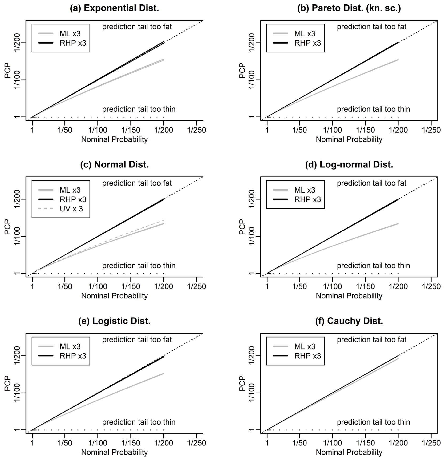
Figure 1 Predictive coverage probability (PCP) versus nominal return probability for predictions generated using maximum likelihood (ML; grey) and right Haar priors (RHP; black) for various distributions. The Pareto distribution has a known scale parameter. The black dots indicate the specified return probabilities at which results were calculated. Each panel shows six lines: three lines showing results from three independent evaluations of the performance of maximum likelihood and three likewise for RHP. Panel (c) shows a third set of three lines (UV; grey, dashed) based on the unbiased estimator for the variance of the normal distribution.

For instance, for the normal distribution example, the return levels corresponding to nominal return periods of 50, 100, 150, and 200 years are exceeded 1.24, 1.35, 1.42, and 1.48 times more often than would be expected and so actually correspond to return periods of 40, 74, 106, and 135 years. For the GEVD, the return levels corresponding to the nominal return periods of 50, 100, 150, and 200 years are exceeded 1.38, 1.69, 1.97, and 2.24 times more often than would be expected and actually correspond to return periods of 36, 59, 76, and 89 years.

For the normal, results based on the unbiased estimator for the standard deviation are very slightly better than those for maximum likelihood but still show considerable reliability bias. For the GEVD, results based on PWM are very slightly better than those for maximum likelihood but again show considerable reliability bias.

From Gerrard and Tsanakas (2011), we know that the maximum likelihood results for the normal and log-normal should be the same, since normal and log-normal are related by an increasing transformation of the random variable. Similarly, the results for exponential and Pareto should be the same.

One way to compensate for the biased predictions generated by the maximum likelihood plug-in method would be to use charts like Figs. 1 and 2 to derive a correction. For instance, for the GEVD, we could use the PCP to relabel the 1-in-200-year event as a 1-in-89-year event. This relabelling approach could be used as the basis for an algorithm for generating less biased predictions, although such an algorithm would be computationally expensive. For the GEVD and GPD, such an algorithm would also still suffer from some reliability bias because the reliability bias depends on the parameters, and the real parameters are unknown. We do not explore the relabelling approach in this study. Rather, we will explore what statistical theory has to say about whether there are computationally inexpensive alternative methods to maximum likelihood for generating predictions that can eliminate or reduce the reliability bias in the first place.

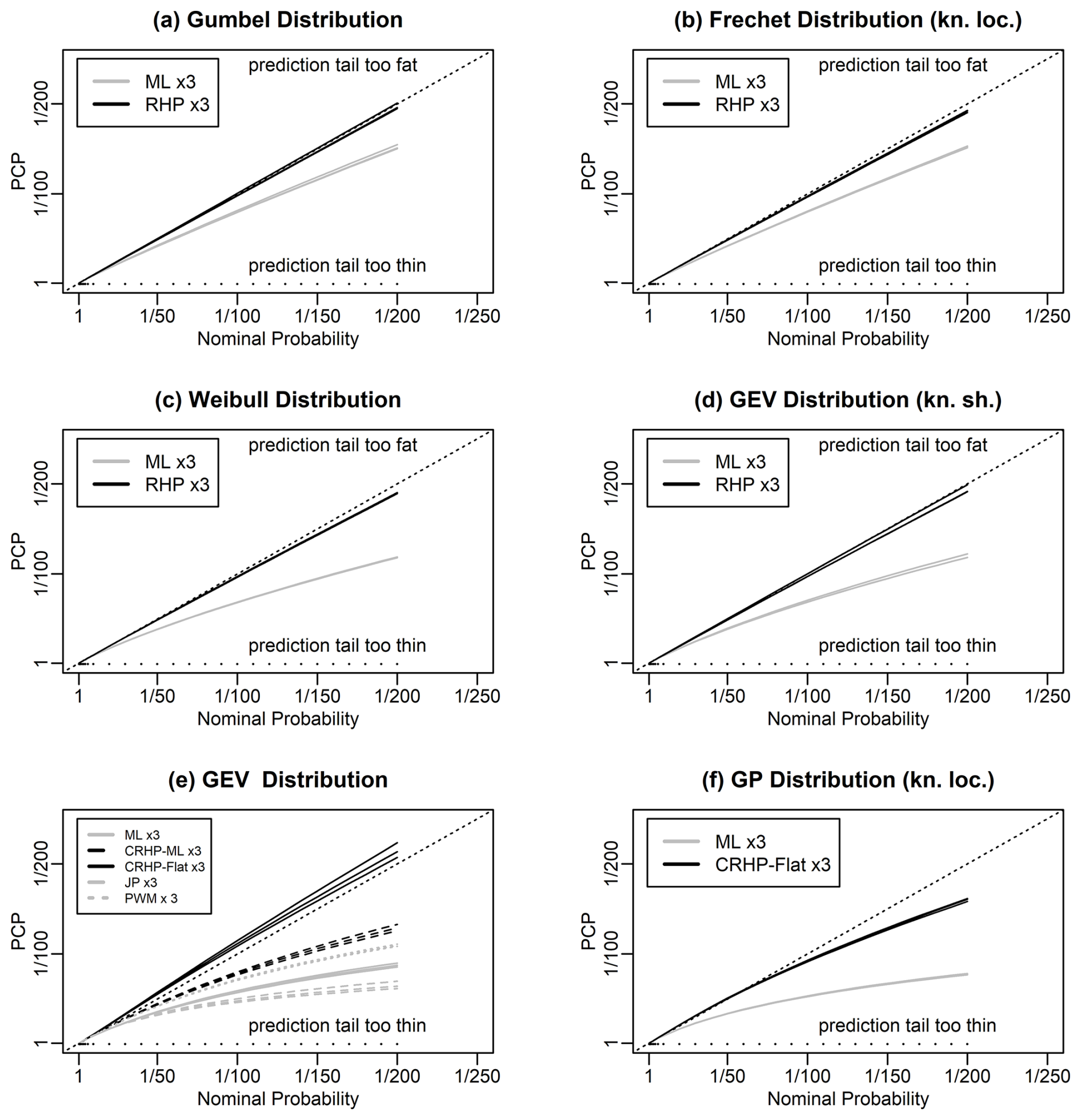
Figure 2 Panels (a)–(d) follow Fig. 1 but for different distributions. The Fréchet distribution has a zero location parameter, and the GEVD in panel (d) has a known shape parameter of −0.25. Panel (e) shows corresponding results for the GEVD for five models: maximum likelihood; a hybrid maximum likelihood/Bayesian prediction, in which we fix the shape parameter to the maximum likelihood estimate and integrate over uncertainty in the location and scale parameters using the conditional right Haar prior (RHP) for the GEVD; Bayesian prediction using the prior given as the product of the conditional RHP for the GEVD with a flat prior for the shape parameter; Jeffreys' prior (JP); and probability weighted moment parameter estimation (PWM). Panel (f) shows corresponding results for the GPD with a zero location parameter for two models: maximum likelihood and a Bayesian prediction using the prior given as the product of the conditional RHP for the GPD with a flat prior for the shape parameter.

3.1 Sampling bias of maximum likelihood predictions

We also evaluate the sampling bias of the probabilities and return levels from our predictions. We do not want, or expect, the sampling bias to be zero, as discussed in the Introduction, since sampling bias is not an indicator of whether predictions are reliable or not. We present the bias simply as a diagnostic that can help with understanding how the predictions are generated. For estimating return values and return probabilities, the sampling biases of the maximum likelihood and Bayesian estimators that we are considering are of the same asymptotic order of n⁻¹ and so tend to zero as the sample size tends to infinity. We evaluate the sampling bias using a modified version of the simulations described above and illustrate it in Figs. S1–S4 in the Supplement. Maximum likelihood gives relatively small but non-zero sampling bias for both the return levels and the return probabilities.

4 A review of predictive probability matching theory

There have been various pieces of statistical research into the question of how to achieve zero reliability bias (i.e. PCP equal to the nominal probability). We use one of the main results from this research, which comes from Fraser (1961), Hora and Buehler (1966), and Severini et al. (2002). This result is that, for a certain class of statistical models known as transitive transformation models, we can achieve zero PCP bias using a Bayesian prediction with the prior set to what is known as the right Haar prior (RHP). This is known as predictive probability matching. The RHP must be determined for each model. This result can be explained in three steps as described in the next three sections.

4.1 Transitive transformation models

If we transform a normally distributed random variable X using the linear transformation $X^{\prime }=a+bX$, then the new random variable X^′ is also normally distributed. If X has a mean and standard deviation (μ,σ), then X^′ has a mean and standard deviation $({\mathit{\mu }}^{\prime }=a+b\mathit{\mu },{\mathit{\sigma }}^{\prime }=b\mathit{\sigma })$, assuming b>0. The set of all these transformations form a group, known as a transformation group. Furthermore, any normally distributed random variable can be transformed to any other normally distributed random variable in this way, and the transformation is invertible, which makes the group of transformations a sharply transitive transformation group (which we abbreviate to transitive transformation group). Not all distributions have transitive transformation groups. For instance, there is no set of transformations over the set of all gamma distributions that form a transitive transformation group.

We refer to those statistical models that are associated with transformations that form a transitive transformation group as transitive transformation models. They are also known homogeneous models (e.g. McCormack and Hoff, 2023). Examples of transitive transformation models are exponential, Pareto with a known scale, Rayleigh, normal with a known location or scale, normal, lognormal with a known location or scale, lognormal, Gumbel, Fréchet with a known location parameter, Weibull, Logistic, Cauchy, Laplace, Lévy, GEVD with a known shape parameter, generalised Pareto distribution (GPD) with a known shape parameter, and any other distribution which has just location and/or scale parameters. Examples of models that are not transitive transformation models are gamma, Pareto, Fréchet, GEVD, GPD with a known location parameter, and GPD.

4.2 Existence of a right Haar prior

If there exists a transformation group acting sharply transitively on a parameter space, then Haar's theorem tells us that there exists what is known as the right Haar prior (RHP) on this parameter space. Haar's theorem was originally proven by the mathematician Alfred Haar in 1933. It is covered in modern textbooks on measure theory and Haar measures such as Diestel and Spalsbury (2014). In fact, we do not have to invoke Haar's theorem to justify our approach since we will derive the RHPs for all the cases in which we need them, and the derivations themselves prove the existence of the RHP for those specific cases. Details of how we derive RHPs are given in the Appendix.

4.3 Predictive probability matching

The RHP can be used to produce a Bayesian predictive distribution for a random variable Y using the standard Bayesian prediction equation given by

$$p\left(y\right|d)={\displaystyle \frac{\int f(y;\mathit{\theta })L(\mathit{\theta };d)\mathit{\pi }\left(\mathit{\theta }\right)\mathrm{d}\mathit{\theta }}{\int L(\mathit{\theta };d)\mathit{\pi }\left(\mathit{\theta }\right)\mathrm{d}\mathit{\theta }}},$$

where p(y|d) is the probability density of the prediction of y given training data d, f(y;θ) is the probability density of a prediction of the random variable Y for given parameter θ, L(θ;d) is the likelihood of the parameter θ given the training data d, and π(θ) is the RHP. This predictive distribution will be probability matching, i.e. will have zero PCP bias. The proof of this result involves the framework described by Fraser (1961), a theorem from Hora and Buehler (1966) that relates Bayesian and frequentist estimates, and the application of this theorem to prediction by Severini et al. (2002).

4.4 Discussion

The Severini et al. (2002) result solves the problem of how to make predictions that are predictive probability matching for transitive transformation models. It therefore tells us how to completely eliminate the PCP bias that we have discussed above for that set of models. We apply the theory to the 10 of our 12 models that are transitive transformation models. The GEVD and GPD with a known location parameter are not transitive transformation models, but we test whether a methodology partly based on the RHP approach can be used to reduce the reliability bias in GEVD and GPD predictions.

4.5 Examples

We now give a number of examples of the RHP for various types of transformation model and some specific distributions.

4.5.1 RHP for location models

Location distributions are distributions with a single parameter μ for which the distribution function is proportional to g(x−μ) for some function g. Examples of families of location distributions are the normal distribution with a known standard deviation, the Gumbel distribution with a known scale parameter, the GEVD with known shape and scale parameters, and the GPD with known shape and scale parameters. The transformation $X^{\prime }=X+a$, ${\mathit{\mu }}^{\prime }=\mathit{\mu }+a$, for any a, then forms a transitive transformation group over the distributions within each family. The RHP in this case is given by π(μ)∝1. The derivation of the location distribution RHP is given in Appendix A.

4.5.2 RHP for scale models

Scale distributions are distributions with a single parameter σ for which the distribution function is proportional to $g(x/\mathit{\sigma })$, for some function g. Examples of families of scale distributions are the exponential, the Weibull with a known shape parameter, the normal with a known location parameter, the Gumbel with a known location parameter, and the GEVD with a known location parameter and a known shape parameter. The transformation $X^{\prime }=bX$, ${\mathit{\sigma }}^{\prime }=b\mathit{\sigma }$, for any b>0, forms a transitive transformation group over scale distributions within each family. The RHP in this case is given by $\mathit{\pi }\left(\mathit{\sigma }\right)\propto \mathrm{1}/\mathit{\sigma }$. The derivation of the scale distribution RHP is given in Appendix A.

4.5.3 RHP for location-scale models

Location-scale distributions are distributions with two parameters (μ,σ) for which the distribution function is proportional to $g\left(\right(x-\mathit{\mu })/\mathit{\sigma })$ for some function g. Examples of families of location-scale distributions are the normal, logistic, Cauchy and Gumbel distributions, and GEVD and GPD with known shape parameters. The transformation $X^{\prime }=a+bX$, ${\mathit{\mu }}^{\prime }=a+b\mathit{\mu }$, ${\mathit{\sigma }}^{\prime }=b\mathit{\sigma }$, for any a and b>0, forms a transitive transformation group over location-scale distributions within each family. The RHP in this case is given by $\mathit{\pi }(\mathit{\mu },\mathit{\sigma })\propto \mathrm{1}/\mathit{\sigma }$. The derivation of the location-scale RHP is given in Appendix A.

The location, scale, and location-scale cases then determine the RHP for all the transitive transformation distributions we are considering using the arguments below.

4.5.4 RHP for the exponential distribution

The exponential is a scale distribution with one parameter λ and exceedance distribution function given by $S\left(x\right)=\exp (-\mathit{\lambda }x)$. Transforming the parameter to $\mathit{\sigma }=\mathrm{1}/\mathit{\lambda }$, to match the form for scale distributions given above, allows us to derive the RHP for the exponential as $\mathit{\pi }\left(\mathit{\lambda }\right)\propto \mathrm{1}/\mathit{\lambda }$. Details of the derivation are given in Appendix B.

4.5.5 RHP for the Pareto distribution with a known scale

The Pareto with a known scale parameter x_m is a distribution with one parameter α, with an exceedance distribution function given by $S\left(x\right)=(x_m/x{)}^{\mathit{\alpha }}$. It is not a location or scale distribution. However, if we transform the random variable to $X^{\prime }=-\log (\log X-\log x_m)$, then X^′ follows a Gumbel distribution with scale=1, which is a location distribution. This allows us to derive the RHP for the Pareto as $\mathit{\pi }\left(\mathit{\alpha }\right)\propto \mathrm{1}/\mathit{\alpha }$. Details of the derivation are given in Appendix C.

4.5.6 RHP for the log-normal distribution

The log-normal is not a location-scale distribution. However, if we transform the random variable to $X^{\prime }=\log X$, then X^′ is normally distributed, and so X^′ does follow a location-scale distribution. Under this transformation, the normal parameters are the same as the log-normal parameters. The RHP for the log-normal is obtained by transforming the RHP for the normal, but since the parameters are the same, the transformation does nothing, and the RHP is the same as for the normal, i.e. $\mathit{\pi }(\mathit{\mu },\mathit{\sigma })\propto \mathrm{1}/\mathit{\sigma }$.

4.5.7 RHP for the Fréchet distribution with a zero location parameter

The Fréchet with a zero location parameter is a distribution with two parameters (s,α) with cumulative distribution function given by $F\left(x\right)=\exp (-(x/s{)}^{-\mathit{\alpha }})$. The Fréchet with a zero location parameter is not a location-scale distribution. However, if we transform the random variable to $X^{\prime }=\log X$, then X^′ follows a Gumbel distribution, which is a location-scale distribution. This allows us to derive the RHP for the Fréchet with a zero location parameter as $\mathit{\pi }(s,\mathit{\alpha })\propto \mathrm{1}/\left(s\mathit{\alpha }\right)$. Details of the derivation are given in Appendix D.

4.5.8 RHP for the Weibull distribution

The Weibull is a distribution with two parameters (k,λ) with exceedance distribution function given by $S\left(x\right)=\exp (-(x/\mathit{\lambda }{)}^k)$. The Weibull is not a location-scale distribution. However, if we transform the random variable to $X^{\prime }=-\log X$, then X^′ follows a Gumbel distribution, which is a location-scale distribution. This allows us to derive the RHP for the Weibull as $\mathit{\pi }(k,\mathit{\lambda })\propto \mathrm{1}/\left(k\mathit{\lambda }\right)$. Details of the derivation are given in Appendix E.

4.5.9 RHP for the GEVD and GPD

The GEVD is a distribution with three parameters $(\mathit{\mu },\mathit{\sigma },\mathit{\xi })$ with a distribution function given by e^−t(x) where for ξ=0, $t\left(x\right)=e^{-(x-\mathit{\mu })/\mathit{\sigma }}$, and otherwise $t\left(x\right)=(\mathrm{1}+\mathit{\xi }((x-\mathit{\mu })/\mathit{\sigma }){)}^{-\mathrm{1}/\mathit{\xi }}$. The parameter ξ is referred to as the shape parameter. For negative values of the shape parameter, the GEVD is a three parameter form of the Weibull; when the shape parameter is zero, the GEVD is equivalent to the Gumbel distribution, and when the shape parameter is positive, the GEVD is a form of the Fréchet distribution. We can create a transformation group for the GEVD using the set of all linear transformations $X^{\prime }=a+bX$, for b>0. However, this transformation group is not transitive since the corresponding transformation of the parameters does not change the value of the shape parameter. Instead, the transformations split the set of GEVDs into multiple subsets (known as orbits in group theory), each with a different value of the shape parameter. The RHP of this transformation group, which we call the conditional RHP (CRHP), does not create probability matching predictions for the distribution when all parameters are unknown. This is because it does not address the need to put a prior on the shape parameter. There is, in fact, no transitive transformation group for the GEVD and hence no RHP. However, the above arguments do show that the GEVD with a known shape parameter is a location-scale model, and hence a transitive transformation model, and so has an RHP of $\mathit{\pi }(\mathit{\mu },\mathit{\sigma })\propto \mathrm{1}/\mathit{\sigma }$.

Similar arguments apply to the GPD with a known location parameter. For the unknown shape parameter there is no RHP, only a CRHP.

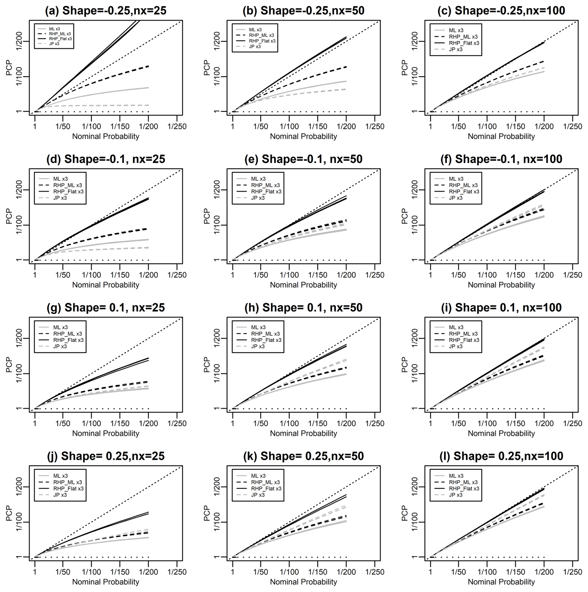
Figure 3 Evaluation of the performance of various methods for predicting GEVD simulated data following the format of Fig. 1. The three columns correspond to sample sizes of 25, 50, and 100, respectively. The four rows correspond to values of the shape parameter of −0.25, −0.1, 0.1, and 0.25, respectively. Four methods are used to make the predictions: (a) maximum likelihood; (b) Bayesian prediction using DMGS with the RHP on the location and scale parameters and using the maximum likelihood value for the shape parameter; (c) Bayesian prediction using DMGS with the RHP on the location and scale parameters and a flat prior on the shape parameter; and (d) Bayesian prediction using DMGS with Jeffreys' prior.

5 Computation of the predictive distributions

Given the theory in the previous section, we now describe methods for producing probability matching predictive distributions for the 10 of our 12 models that are transitive transformation models. For each model we consider how to evaluate the Bayesian prediction integral, given the RHP for that model, and where possible, we use analytic solutions. However, in many cases, analytic solutions are not possible. Methods for evaluating the Bayesian prediction integral, in the absence of analytical solutions, include numerical quadrature, importance sampling, rejection sampling schemes such as ratio-of-uniforms sampling (RUST) (Wakefield et al., 1991; Northrop, 2023), and Monte Carlo Markov chain (MCMC) (see, for example, textbooks such as Bailer-Jones, 2017). They each have advantages and disadvantages, depending on the problem being addressed, but none are completely straightforward to use. For instance, although MCMC is available in many software packages, using it requires an understanding of burn-in and convergence. As a simpler approach, that requires less understanding, we use a novel method for evaluating the Bayesian prediction integral, taken from the Datta et al. (2000) study on approximate predictive probability matching. Datta et al. (2000) treat the maximum likelihood plug-in prediction as the first term in an asymptotic expansion and then also derive the second term. Equation (2.1) in their paper gives the following expression for the predictive probability density:

$$\begin{array}{}\text{(2)}& \begin{array}{rl}& p\left(y\right|d)=f(y;\widehat{\mathit{\theta }})\\ & {\displaystyle \frac{\mathrm{1}}{\mathrm{2}n}}\left[c^{\mathrm{st}}\left\{c^{\mathrm{jr}}{a}_{\mathrm{jrs}}+{\displaystyle \frac{\mathrm{2}{\mathit{\pi }}_s\left(\widehat{\mathit{\theta }}\right)}{\mathit{\pi }\left(\widehat{\mathit{\theta }}\right)}}\right\}{f}_t(y;\widehat{\mathit{\theta }})+c^{\mathrm{jr}}{f}_{\mathrm{jr}}(y;\widehat{\mathit{\theta }})\right]\\ & +o\left(n^{-\mathrm{1}}\right),\end{array}\end{array}$$

where c_st and a_jrs are, respectively, the negative inverse of the matrix of second-order and the tensor of third-order partial derivatives of the log-likelihood, both evaluated at $\widehat{\mathit{\theta }}$; π(θ) is the prior density; π_s(θ) is the vector of first-order partial derivatives of π(θ); and f_t(y;θ) and f_jr(y;θ) are, respectively, the vector of first-order and the matrix of second-order partial derivatives of f(y;θ), where the partial derivatives are all with respect to the parameters. The summation convention has been used to simplify this expression.

Equation (3.3) in Datta et al. (2000) then gives a corresponding first-order expression for the predicted quantiles as a function of the exceedance probability:

$$\begin{array}{}\text{(3)}& \begin{array}{rl}& h(\mathit{\pi },\mathit{\alpha })=q(\widehat{\mathit{\theta }},\mathit{\alpha })+{\displaystyle \frac{\mathrm{1}}{nf\left(q\right(\widehat{\mathit{\theta }},\mathit{\alpha });\widehat{\mathit{\theta }})}}\\ & \left[c^{\mathrm{st}}\left\{{\displaystyle \frac{\mathrm{1}}{\mathrm{2}}}{c}^{\mathrm{jr}}{a}_{\mathrm{jrs}}+{\displaystyle \frac{{\mathit{\pi }}_s\left(\widehat{\mathit{\theta }}\right)}{\mathit{\pi }\left(\widehat{\mathit{\theta }}\right)}}\right\}{\mathit{\mu }}_t(\widehat{\mathit{\theta }},\mathit{\alpha })+{\displaystyle \frac{\mathrm{1}}{\mathrm{2}}}{c}^{\mathrm{jr}}{\mathit{\mu }}_{\mathrm{jr}}(\widehat{\mathit{\theta }},\mathit{\alpha })\right],\end{array}\end{array}$$

where h(π,α) is the predictive quantile given prior π and exceedance probability α; ${\mathit{\mu }}_t(\mathit{\theta },\mathit{\alpha })=-F_t\left(q\right(\mathit{\theta },\mathit{\alpha });\mathit{\theta })$ and ${\mathit{\mu }}_{\mathrm{jr}}(\mathit{\theta },\mathit{\alpha })=-F_{\mathrm{jr}}\left(q\right(\mathit{\theta },\mathit{\alpha });\mathit{\theta })$, where F_t(y;θ) and F_jr(y;θ) are, respectively, the first-order and second-order partial derivatives of F(y;θ) with respect to the parameters. These definitions of μ_t and μ_jr are different but equivalent to the definitions (3.2) given in Datta et al. (2000).

Although apparently complex, the evaluation of Eqs. (2) and (3) is straightforward as it involves only the differentiation of the likelihood, prior, density and distribution function, and matrix multiplication. We refer to the idea of using this equation to estimate predictive densities and quantiles as the DMGS method (after the initials of the authors of Datta et al., 2000). Relative to the standard numerical methods for evaluating the Bayesian prediction integral, the DMGS method has advantages and disadvantages:

• a.

  DMGS is straightforward to automate (i.e. to run for many cases without human intervention). For our purposes, automation is important since we are running many thousands of test cases for many distributions and are developing software libraries.

• b.

  DMGS is faster than the numerical integration methods. Speed is important in our application since our simulation tests involve many evaluations.

• c.

  Equation (3) gives the quantiles we require directly as a function of the exceedance probabilities.

• d.

  DMGS will be less accurate than a method that evaluates the full integral since it is only a first-order approximation. We assess whether it is a good approximation or not using the results from our simulation testing. High accuracy is less important for us, given the uncertainties involved in all other steps of the estimation of extreme weather return periods.

For two parameter distributions, our application of the DMGS equations involve the numerical evaluation of the various terms in Eq. (3). Here the vectors ${\mathit{\mu }}_t(\widehat{\mathit{\theta }},\mathit{\alpha })$ and ${\mathit{\pi }}_s\left(\widehat{\mathit{\theta }}\right)$ have two components, c_st and ${\mathit{\mu }}_{\mathrm{jr}}(\widehat{\mathit{\theta }},\mathit{\alpha })$ are 2×2 matrices with three unique terms, and a_jrs is a $\mathrm{2}\times \mathrm{2}\times \mathrm{2}$ tensor with four unique terms. For three-parameter distributions, the vectors have 3 components, the matrices become 3×3 matrices with 6 unique terms, and the tensor becomes a $\mathrm{3}\times \mathrm{3}\times \mathrm{3}$ tensor with 10 unique terms. For four-parameter distributions, the vectors have 4 components, the matrices become 4×4 matrices with 10 unique terms, and the tensor becomes a $\mathrm{4}\times \mathrm{4}\times \mathrm{4}$ tensor with 20 unique terms.

5.1 Specific distributions

We now describe how we evaluate the Bayesian prediction integral with the prior set to the RHP for 10 of our models that are transitive transformation models. For the GEVD, and GPD with a known location parameter, we describe a number of alternative approaches for generating predictions. An evaluation of the properties of the resulting return period predictions is given in Figs. 1 and 2 in black.

5.1.1 Prediction for the exponential distribution

For the exponential, the Bayesian prediction integral can be solved exactly, giving quantile predictions of the form

$$\widehat{q}\left(\mathit{\alpha }\right)=s\left({\mathit{\alpha }}^{-\mathrm{1}/n}-\mathrm{1}\right),$$

where x_i is the historical data and $s={\sum }_{i=\mathrm{1}}^n{x}_i$. Figure 1a shows that these predictions are exactly predictive probability matching, up to the accuracy of our simulation tests, as expected from the theory.

5.1.2 Prediction for the Pareto distribution with a known scale

For the Pareto with a known scale, the Bayesian prediction integral can be solved exactly, giving quantile predictions of the form

$$\widehat{q}\left(\mathit{\alpha }\right)=\exp \left(s\left({\mathit{\alpha }}^{-\mathrm{1}/n}-\mathrm{1}\right)\right).$$

Figure 1b shows that these predictions are exactly predictive probability matching, up to the accuracy of our simulation tests, as expected.

5.1.3 Prediction for the normal distribution

The normal distribution, when parameterised using the mean μ and standard deviation σ, is a location-scale distribution, and so the RHP is given by $\mathit{\pi }(\mathit{\mu },\mathit{\sigma })\propto \mathrm{1}/\mathit{\sigma }$. If the normal distribution is parameterised differently (for instance, using the variance or the inverse of the standard deviation or the inverse of the variance), then the RHP must be transformed using the rule for transforming probability densities. This prior was proposed as an appropriate prior for the normal distribution by Jeffreys (1961) before the development of the RHP theory and is often known as Jeffreys' independence prior for the normal distribution.

The Bayesian prediction integral with this prior can be solved exactly (see, for instance, Lee, 2012), giving quantile predictions of the form

$$\widehat{q}\left(\mathit{\alpha }\right)=\stackrel{\mathrm{‾}}{x}+\widehat{\mathit{\sigma }}\sqrt{(\mathrm{1}+\mathrm{1}/n)}{Q}_t(\mathrm{1}-\mathit{\alpha },n-\mathrm{1}),$$

where $\stackrel{\mathrm{‾}}{x}$ is the mean of x_i, $\widehat{\mathit{\sigma }}$ is the square root of the usual unbiased estimator of the variance, with the denominator n−1, and $Q_t(\mathrm{1}-\mathit{\alpha },n-\mathrm{1})$ is the set of quantiles of the t distribution with n−1 degrees of freedom at a probability of 1−α.

By comparison with corresponding predictions for the normal distribution with a known mean and a known variance (see, e.g. Lee, 2012), it can be seen that the $\sqrt{(\mathrm{1}+\mathrm{1}/n)}$ term arises because of the uncertainty around the mean parameter, while the t distribution arises because of the uncertainty around the standard deviation parameter. This distribution is identical to the confidence distribution for the normal distribution (see, e.g. Wasserman, 2003). Figure 1c shows that these predictions are exactly predictive probability matching, up to the accuracy of our simulation tests, as expected.

5.1.4 Prediction for the log-normal distribution

For the log-normal distribution, the Bayesian prediction integral can be solved exactly by transforming the random variable to that of a normal distribution using the normal distribution solution and transforming back. Figure 1d shows that these predictions are exactly predictive probability matching, up to the accuracy of our simulation tests, as expected.

5.1.5 Prediction for the logistic, Cauchy, and Gumbel distributions

The logistic distribution with the distribution function $F\left(x\right)=(\mathrm{1}+\exp (-(x-\mathit{\mu })/\mathit{\sigma }){)}^{-\mathrm{1}}$, the Cauchy distribution with the density function $f\left(x\right)=\left(\mathit{\pi }\mathit{\sigma }\right[\mathrm{1}+\left(\right(x-\mathit{\mu })/\mathit{\sigma }{)}^{\mathrm{2}}]{)}^{-\mathrm{1}}$, and the Gumbel distribution with the distribution function $F\left(x\right)=\exp \left(-\exp \left(-\left((x-\mathit{\mu })/\mathit{\sigma }\right)\right)\right)$ are all location-scale distributions and so all have the RHP given by $\mathit{\pi }(\mathit{\mu },\mathit{\sigma })\propto \mathrm{1}/\mathit{\sigma }$.

There are, however, no known closed-form solutions for the Bayesian prediction integrals in these cases, and so we use the DMGS method. Figures 1e, f and 2a show our numerical evaluation of the PCP calculated using the DMGS method. At the accuracy of the simulations, the predictions appear to be exactly predictive probability matching. The impact of the approximation used in the DMGS method is not apparent. We conclude that the DMGS method is sufficiently accurate for our purposes for these distributions for this sample size.

5.1.6 Prediction for the Fréchet distribution with a zero location parameter, Weibull distribution, and GEVD with a known shape parameter

There are no known closed-form solutions for the Bayesian prediction integrals in these cases, and so we use the DMGS method. Figure 2b, c, d show our numerical evaluation of the PCP calculated using the DMGS method. There are slight biases, with the values of the PCP being slightly higher than the nominal probabilities. These biases are because of the first-order approximation used in the DMGS method. The biases are much smaller than the bias from using maximum likelihood, and we conclude that the DMGS method is sufficiently accurate for our purposes. For other purposes, or smaller sample sizes, it may be necessary to use a different method to evaluate the integral, such as RUST or MCMC, to achieve more accurate results.

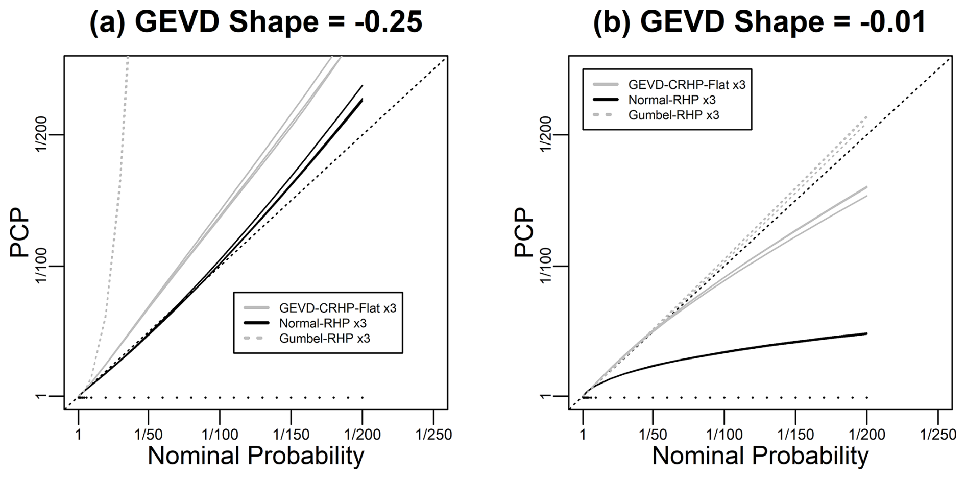
Figure 4 Evaluation of the performance of three methods for predicting GEVD simulated data, for a sample size of 25, following the format of Fig. 1. The three methods are all Bayesian predictions based on the GEVD, the normal, and the Gumbel, respectively. The prior for the GEVD is the CRHP-flat prior, while the priors for the normal and Gumbel are the RHP. Panel (a) considers data simulated with a shape parameter of −0.25, and panel (b) considers data simulated with a shape parameter of −0.01.

5.1.7 Prediction for the GEVD

The GEVD with unknown shape parameter is not a transitive transformation model, as discussed above, and hence the RHP approach does not give a method for making probability matching predictions. There is currently a lack of theory that might help, and the only way to find methods that give predictions that are close to probability matching is trial and error. There are many possible approaches, and we have investigated the following three methods in addition to maximum likelihood:

• a.

  a hybrid maximum likelihood/Bayesian prediction, in which we fix the shape parameter to the maximum likelihood estimate and integrate over the uncertainty in the location and scale parameters with the prior set to the CRHP for the GEVD, which we refer to as the CRHP-ML method;

• b.

  Bayesian prediction using the CRHP for the GEVD, along with a flat prior on the shape parameter, which we refer to as the CRHP-flat method; and

• c.

  Bayesian prediction using Jeffreys' prior, which has the property that it is invariant to parameter transformation.

In all three cases, we calculate the predictive quantiles using the DMGS method. Figure 2e shows that the best results come from the CRHP-flat method. This method gives values of the PCP which are slightly lower than the nominal probability. The CRHP-ML method outperforms maximum likelihood but still shows a large reliability bias, while Jeffreys' prior does not perform as well as maximum likelihood.

Figure 3 explores the performance of our four methods for predicting the GEVD as a function of the sample size and shape parameter for sample sizes ranging from 25 to 100 and values of the shape parameter ranging from −0.25 to 0.25. The CRHP-flat method is consistently the best method. This method performs very well for a sample size of 100 and appears to give near-perfect probability matching. It performs less well for a sample size of 25. The results in this figure show that the reliability bias from all methods is reduced as the sample size increases.

The poor performance of the CRHP-flat method for small sample sizes motivates us to explore whether alternative distribution shapes, for which there is an RHP, might be better for predicting GEVD data in some cases. Figure 4 shows results from a numerical experiment in which we simulate GEVD data and attempt to predict it using Bayesian methods based on GEVD with a CRHP-flat prior and normal and Gumbel distributions with the RHP. When the simulated data is based on a shape parameter of −0.25, predictions based on the normal distribution with the RHP give a better prediction than the GEVD with the CRHP-flat prior. When the simulated data is based on a shape parameter of −0.01, predictions based on the Gumbel distribution with the RHP give a better prediction than the GEVD with the CRHP-flat prior. These are just suggestive results, but they add weight to the argument given in Sect. 2 that it may make sense to test a number of models when predicting maxima rather than just using only the GEVD.

5.1.8 Prediction for the GPD with a known location parameter

The GPD with a known location parameter is also not a transitive transformation model. Figure 2f shows results from testing the CRHP-flat method. This method gives PCP values that are slightly higher than the nominal probability at long return periods but which are much more accurate than maximum likelihood in this case.

Figure 5 explores the performance of two methods for predicting the GPD with a known location parameter as a function of the sample size and shape parameter for sample sizes ranging from 25 to 100 and values of the shape parameter ranging from 0 to 0.6. The CRHP-flat method is consistently the best method. As for the GEVD, this method performs very well for a sample size of 100 and appears to give near-perfect probability matching. It performs less well for a sample size of 25.

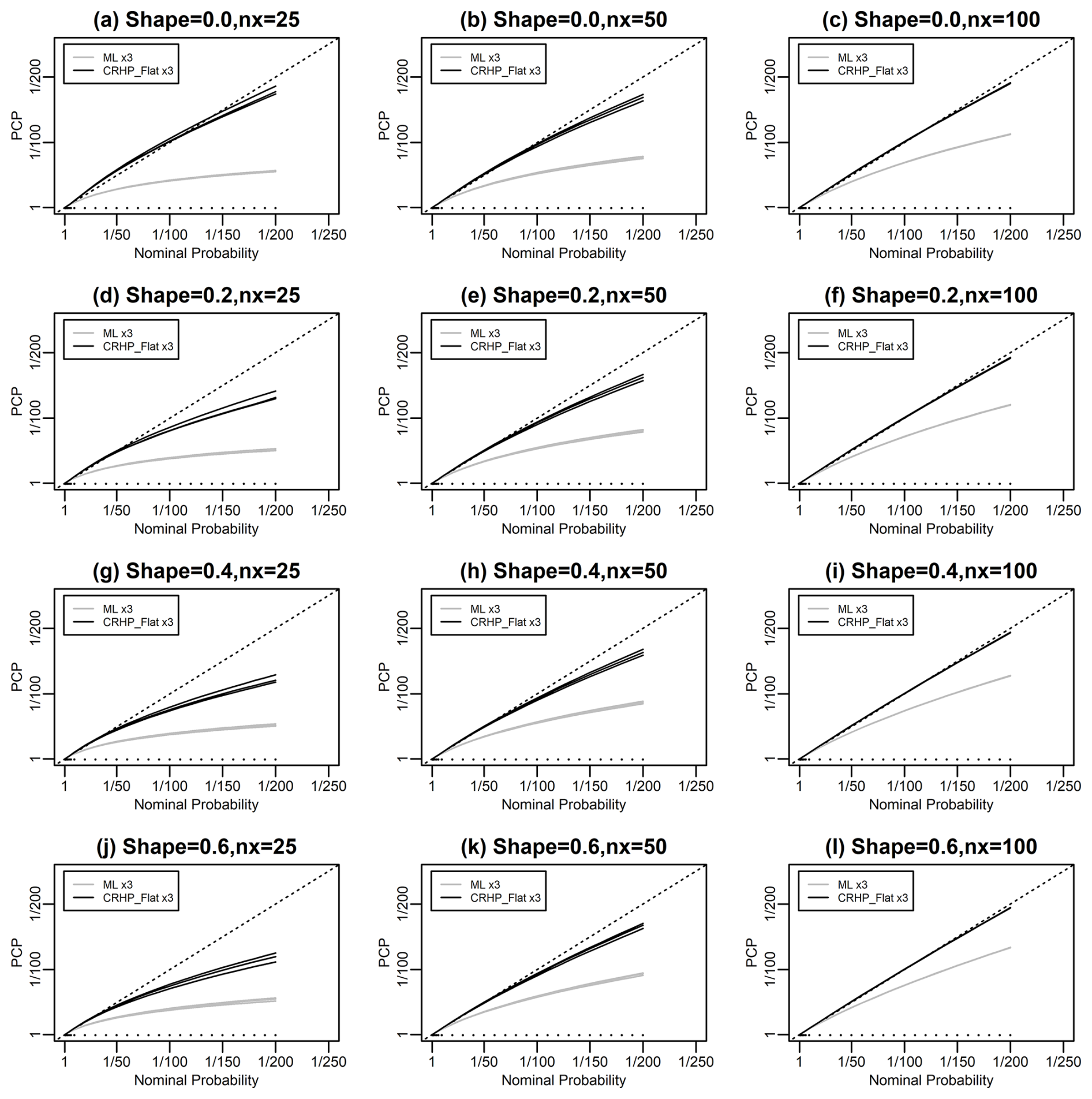
Figure 5 Similar to Fig. 3 but now for data simulated using the GPD. The three columns correspond to sample sizes of 25, 50, and 100, respectively. The four rows correspond to values of the shape parameter of 0, 0.2, 0.4, and 0.6, respectively. Two methods are used to make the predictions: (a) maximum likelihood; and (b) Bayesian prediction using DMGS with the CRHP on the location and scale parameters and a flat prior on the shape parameter.

5.2 Sampling bias of Bayesian predictions

We can also consider the sampling bias of our Bayesian estimators of the return value and return probability. Results are shown in Figs. S1–S4. Evaluating the return probability bias requires calculating exceedance probabilities. For all except the GEVD and GPD, we evaluate the exceedance probabilities using an asymptotic expansion derived from the density expansion given in Datta et al. (2000). However, this asymptotic expansion is not suitable for evaluating densities and probabilities for the GEVD and GPD because the support of these models depends on the parameter values, and so we evaluate the exceedance probabilities using RUST instead. For the return value estimators, we see that in the upper tail the Bayesian estimators all have positive sampling bias and that the magnitude of the biases is larger than that of the maximum likelihood biases. For the return probability estimators, we see that the sampling biases are of a similar size to the maximum likelihood sampling biases. That Bayesian predictions show sampling biases in this way is well known (see, e.g. Bernardo and Smith, 1993; Gelman et al., 1995), and is not related to the performance of the predictions in terms of reliability. For the RHP models, one could say that these biases are necessary in order to achieve reliable predictions, and it seems likely that they are necessary to achieve approximate reliability for the non-RHP models too.

6 Extension to modelling trends

In many cases, extreme weather return periods are estimated in the presence of a trend due to climate change. The best way to capture a trend is to use a single statistical model that encompasses both the trend and the distribution around the trend. Any of the statistical models we have discussed above can be generalised to include a trend by adding a predictor to any of the parameters. For instance, a location parameter μ can be replaced with a linear function of a predictor r_i, giving ${\mathit{\mu }}_i=\mathit{\alpha }+\mathit{\beta }{r}_i$. For a location-scale model with a trend, the transformation $X_i^{\prime }=a+b{X}_i+c{r}_i$, ${\mathit{\alpha }}^{\prime }=a+b\mathit{\alpha },{\mathit{\beta }}^{\prime }=b\mathit{\beta }+c,{\mathit{\sigma }}^{\prime }=b\mathit{\sigma }$, for any a,c and b>0, forms a transitive transformation group over the distributions in the family.

We apply linear trends to the location parameters of the following six models: normal, log-normal, logistic, Cauchy, Gumbel, and GEVD. For the GEVD, we additionally apply a log-linear trend to the scale parameter and a linear trend to the shape parameter. The predictors r_i would typically be either time or global mean surface temperature. In each case, adding a predictor in this way adds an extra parameter to the model since the original parameter is replaced by two parameters. The derivation for the RHP for linear predictors on the location parameter is given in Appendix F, and the RHPs do not change in any of the six cases relative to the same model without the trend. The details of how we make predictions for the six distributions with trends are as follows.

Figure 6 As Fig. 1 but for models with trends, i.e. predictors, on the location parameter.

6.1 Normal distribution with a trend

For the normal with a trend, the RHP prediction for the point r₀ is given by

$$\widehat{q}\left(\mathit{\alpha }\right)=\stackrel{\mathrm{‾}}{x}+\widehat{\mathit{\sigma }}\sqrt{(\mathrm{1}+\mathrm{1}/n+R_{\mathrm{0}}/R)}{Q}_t(\mathrm{1}-\mathit{\alpha },n-\mathrm{2}),$$

where the unbiased estimator for the variance ${\widehat{\mathit{\sigma }}}^{\mathrm{2}}$ uses n−2 in the denominator, $R_{\mathrm{0}}=(r_{\mathrm{0}}-\stackrel{\mathrm{‾}}{r}{)}^{\mathrm{2}}$, and $R={\sum }_{i=\mathrm{1}}^n(r_i-\stackrel{\mathrm{‾}}{r}{)}^{\mathrm{2}}$.

6.2 Log-normal distribution with a trend

For the log-normal with a trend, the RHP prediction can be produced by taking the log of the data x_i, producing the RHP prediction for the normal distribution with a trend and taking the inverse log of the prediction.

6.3 Logistic, Cauchy, and Gumbel distributions with a trend

For the logistic, Cauchy, and Gumbel with trends, there is no analytic solution for the prediction, and we use the DMGS approach.

6.4 GEVD with a trend

For the GEVD, we consider models with trends on the location (GEV1); on the location and the scale (GEV2); and on the location, scale, and shape (GEV3). In all cases, we make predictions using maximum likelihood and a CRHP-flat prior. We do not consider the other two models that were considered for the GEVD without a trend, given their poor performance. We use the DMGS approach for the Bayesian integral.

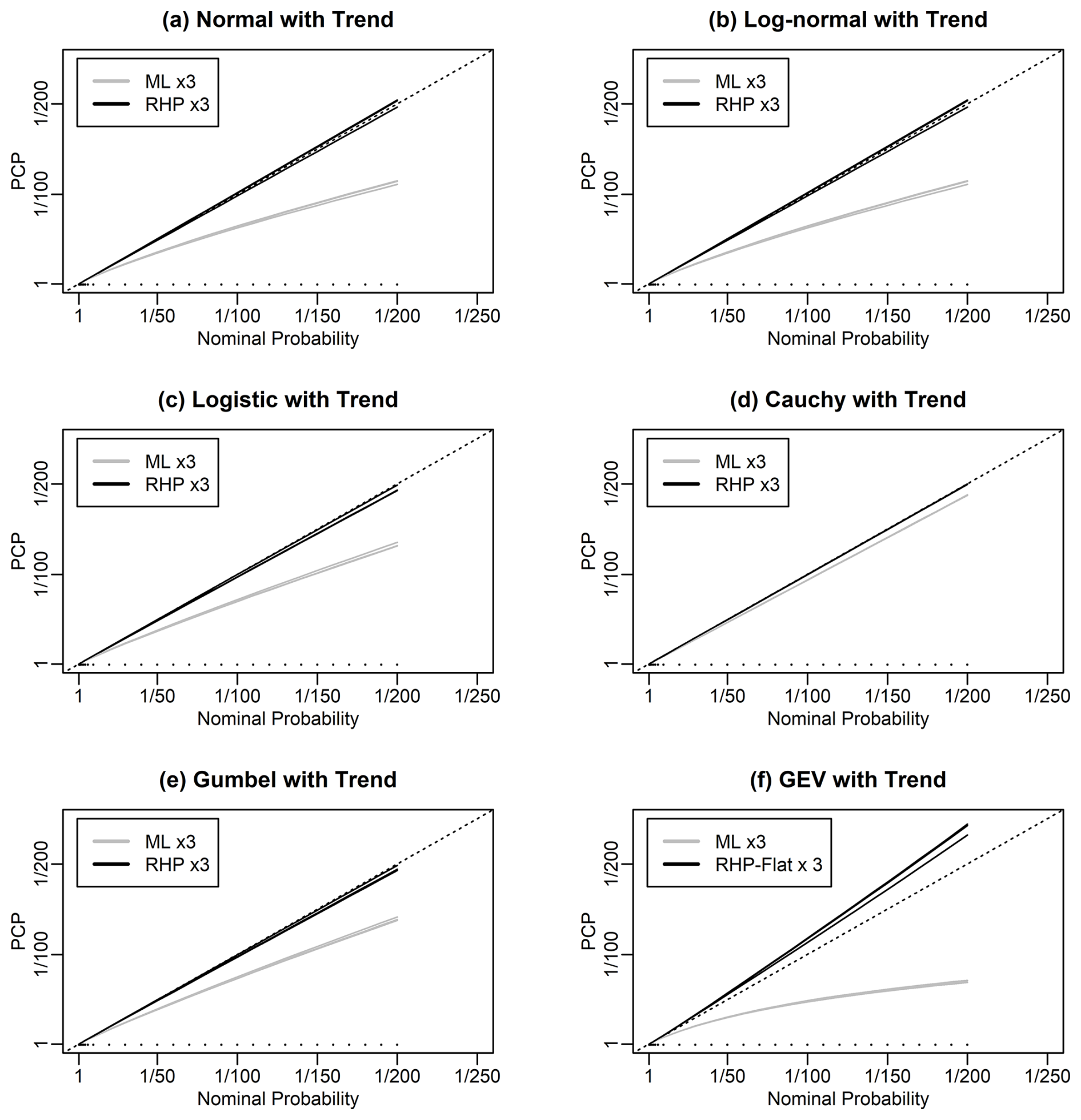
6.5 Numerical testing of trend models

We test these trend models using simulations, as for the non-trend models. In all cases, the trend is set to a slope of 1 in 50 years, although the PCP results do not depend on the size of the slope. Results are shown in Fig. 6 and show that the normal, log-normal, logistic, Cauchy, and Gumbel with a trend models show poor probability matching when using maximum likelihood and good probability matching when using the RHP. The GEVD with trend shows poor probability matching when using maximum likelihood. The CRHP-flat method performs much better than maximum likelihood.

In Figs. S5–S7, we give results for the performance of maximum likelihood and the CRHP-flat method for the GEV1, GEV2, and GEV3 models as a function of the sample size and shape parameter. We see that the CRHP-flat method always beats maximum likelihood and once again performs very well for a sample size of 100. We see that the reliability biases increase as more predictors are added.

7 De Bilt example

We now revisit the De Bilt example that has previously been discussed in Philip et al. (2020), van Oldenborgh et al. (2021), and van Oldenborgh et al. (2022). This example considers 118 or more years of annual maximum temperature data from De Bilt (in our case, we use 122 years of data).

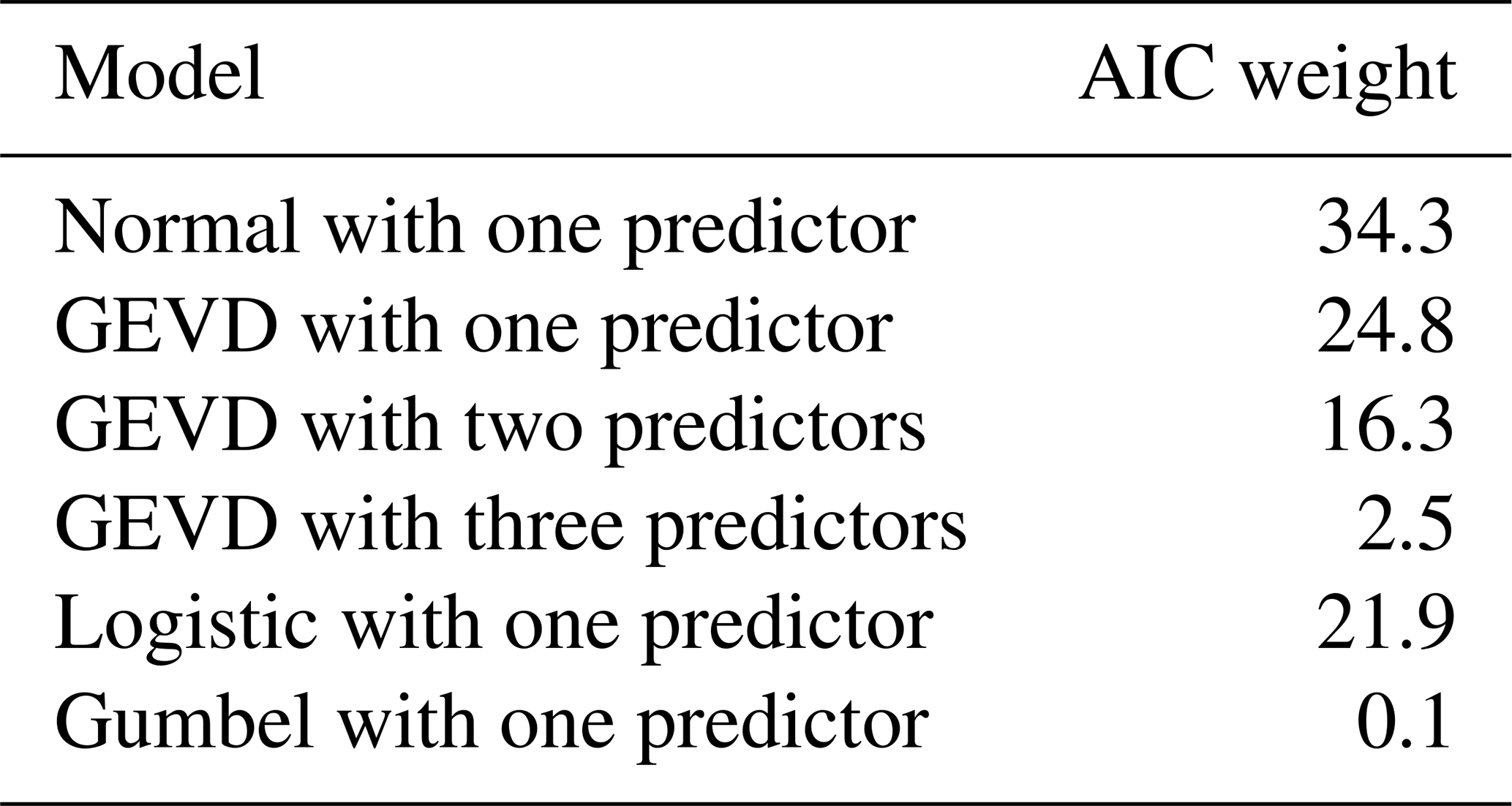
Table 1 Model selection AIC weights for six models applied to De Bilt historical maximum temperatures. The weights sum to 100 (before rounding).

We use the model selection philosophy for modelling extremes, as discussed in Sect. 2, in which we consider multiple models rather than just relying solely on the GEVD. We consider the following six models: normal with a linear predictor on the mean, GEV1, GEV2, GEV3, logistic with a linear predictor on the location, and Gumbel with a linear predictor on the location. We use global mean surface temperature for the predictors. For the normal, logistic, and Gumbel, we consider both maximum likelihood (ML) and RHP predictions. For the GEVD models, we consider maximum likelihood and CRHP-flat predictions. The ML models are only included for model selection, and as points of comparison, since we already know from our simulation results that they do not give good extrapolation of extremes and so are not appropriate models. In all the models, we merge the steps of trend and distribution modelling.

For the GEV1 model, the maximum likelihood parameter estimates are as follows: location =23.2, trend slope =3.13, scale =1.66, and shape $=-\mathrm{0.32}$. For this value of the shape parameter, the GEVD has a somewhat similar shape to the normal distribution. For model selection among the maximum likelihood models, we calculate AIC weights. Table 1 shows that the normal model gets the highest weight, followed by the GEV1 model and then the logistic model. GEV2 and GEV3 get lower AIC weights, and the Gumbel gets almost zero weight, implying that it does not fit the historical data well at all.

We see that this is an example where the model selection scores favour a model for maxima which is not the GEVD. Comparing the likelihoods for the normal and GEV1 models shows that the GEV1 has a higher likelihood and the normal only has a better AIC score because of the compensation for having fewer parameters. The AIC model selection is therefore favouring normal over GEV1 because it considers GEV1 to be overfitted relative to the normal.

Our decision of which model or models to select in this case is a subjective one based on the model selection scores, extreme value theory, and simulation results presented earlier. Different scientists may put a different emphasis on these three factors. The model selection scores assess the overall agreement between the distribution shape and the data, while the simulation results assess the ability to extrapolate into the tail, which is not assessed by the model selection scores. We conclude that the best model to use in this case, of the 10 we are considering, would be the normal RHP model since the normal has the best model selection scores, and using the RHP version should give good extrapolation in the tail. The second- and third-best models are the GEV1 with a CRHP-flat prior and the logistic RHP models since these models both have reasonably good model selection scores and would be expected to extrapolate well into the tail. The best three models all perform well, and considering all three is useful as it gives an indication of the level of model uncertainty.

Figure 7 shows predictions from the normal and GEVD methods for 1901 and 2022 climates. We see that the normal models give higher temperatures for a known return period (or shorter return periods for a known temperature) than the corresponding GEV1 models.

In the 1901 climate, the 2018 heatwave has a return period much longer than any we have calculated in the normal, logistic, or GEV1 models, emphasising how drastically climate has changed between 1901 and 2018. In the 2022 climate, in the normal RHP model (the first of our selected models), the 2018 heatwave has a return period of 44 years. In the second and third of our selected models, the GEV1 CRHP-flat prior and logistic RHP models, the heatwave has return periods of 34 and 52 years. All of these return periods are shorter than the return period from the GEVD ML model, which is 90 years.

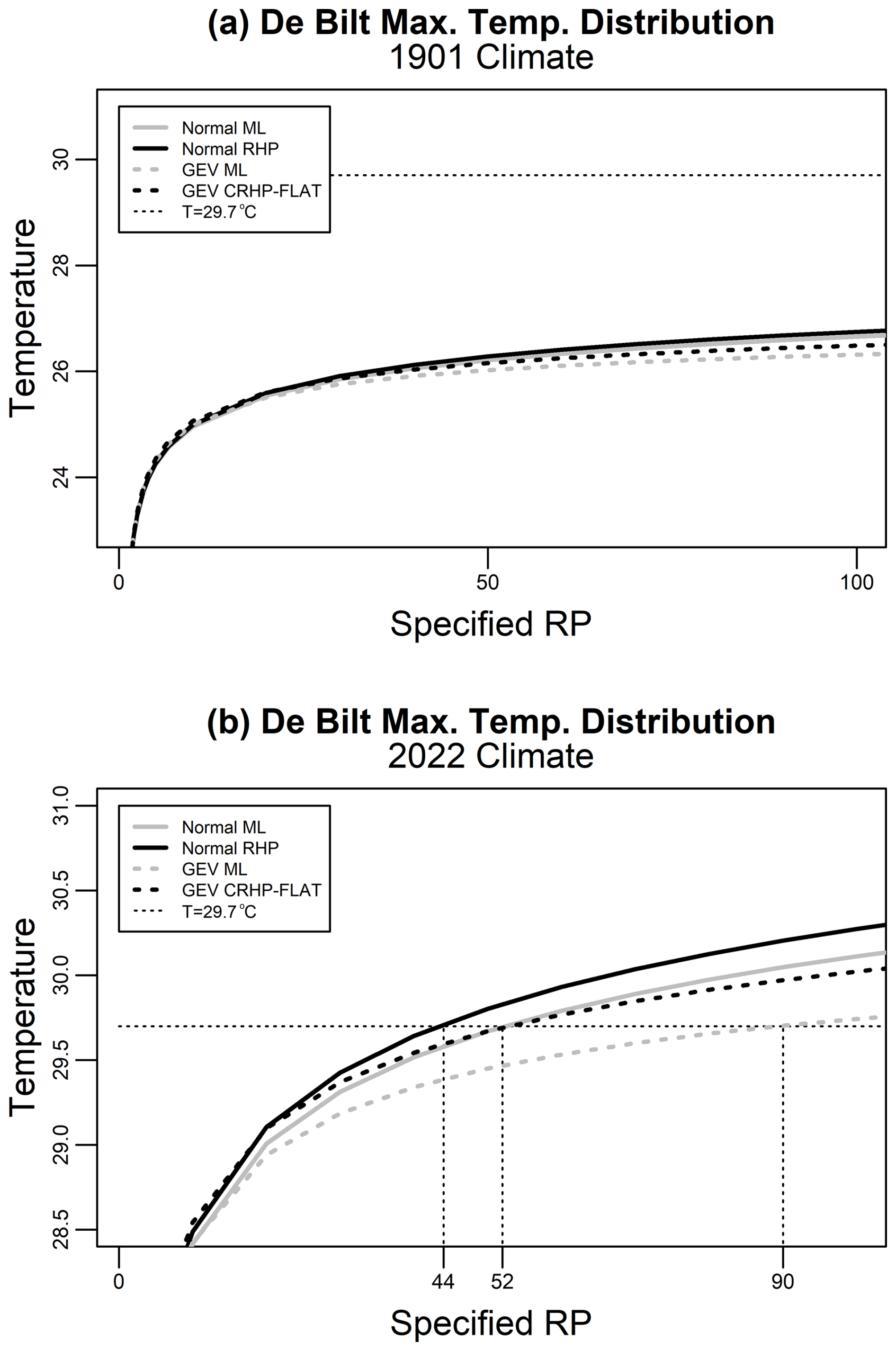
Figure 7 Return periods for maximum temperature at De Bilt based on four different statistical methods for (a) 1901 climate and (b) 2022 climate. The location parameters are all modelled with global mean surface temperature as a linear predictor. The models are normal (solid lines) and GEVD (dashed lines) based on maximum likelihood (grey) or Bayesian methods (black). The normal models achieve the best model selection scores. The return periods of the 2018 heatwave of 29.7 °C in the 2022 climate are shown by vertical dashed lines.

7.1 Uncertainty intervals

Studies that have used maximum likelihood to estimate extremes often use a parametric bootstrap method to generate confidence intervals around the estimated return probabilities. In Fig. S8, we show results for 90 % confidence intervals generated in this way for the GEV1 maximum likelihood model and compare them with the GEV1 CRHP-flat model return probabilities. We see that at short return periods, the Bayesian return probabilities are greater than the maximum likelihood return probabilities but still lie within the range of the confidence intervals. However, at longer return periods, beyond around 1500 years, the Bayesian return probabilities lie outside the confidence intervals. This can readily be understood as the Bayesian predictive distributions have fatter tails than the underlying distributions. For instance, the predictive distribution for the normal distribution is a t distribution, which has fatter tails than the normal, and the predictive distribution for the exponential distribution is a Pareto distribution, which has fatter tails than the exponential. Similarly, for the GEVD, the predictive distribution is also fatter-tailed. The confidence intervals for the maximum likelihood GEVD are based on GEVDs with different parameter values. However, any GEVD, with any parameter values, will always ultimately be overtaken by the predictive distribution we are generating because of the fatter tails.

For our Bayesian prediction, uncertainty intervals can be created by sampling from the posterior distribution. We have generated Bayesian intervals in this way using RUST. The results are also shown in Fig. S9.

8 Conclusions

We have compared statistical predictions of extremes that propagate parameter uncertainty with statistical predictions based on maximum likelihood, in the context of univariate parametric statistical models. This is motivated by a number of recent studies which have used statistical models to estimate extreme weather return periods using maximum likelihood, including Philip et al. (2022), Otto et al. (2023), Rivera et al. (2023), Thompson et al. (2023), Vautard et al. (2023), Zachariah et al. (2023), and van Oldenborgh et al. (2022).

We have used simulations to show that if the statistical model is being fitted using maximum likelihood to 50 years of data, then estimated return levels corresponding to return periods of around 25 years and above will be exceeded materially more often than the return period suggests. We call this discrepancy between the probability of exceeding a predicted quantile and the probability implied by the nominal return period of the prediction a reliability bias. The reliability bias gets worse as the return period increases. The degree of the reliability bias varies from distribution to distribution, but of the distributions we have tested, it is the worst for the GEVD and GPD. For the GEVD, return level estimates corresponding to return periods of 200 years are exceeded more than once in every 100 years rather than once every 200 years as one would expect.

We have explored using objective priors that are chosen to reduce this reliability bias, which we call calibrating priors. For certain statistical models, known as transitive transformation models, it is possible to derive a Bayesian prior, known as the right Haar prior (RHP), that can be used to make objective Bayesian predictions that give predictions without reliability bias (assuming that the statistical model is correct). We have given the RHP for a number of commonly used distributions: the exponential distribution, Pareto distribution with a known scale parameter, normal distribution, log-normal distribution, logistic distribution, Cauchy distribution, Gumbel distribution, Fréchet distribution with a known location parameter, Weibull distribution, and GEVD with a known shape parameter.

The situation for non-transitive transformation models, such as the GEVD and GPD, is more complex. There is no RHP for non-transitive transformation models, and it is unclear as to what the best method is for making predictions. We have therefore resorted to trial and error, and have tested four methods for predicting the GEVD and two methods for predicting the GPD. We find a Bayesian method that gives reasonably good predictive probability matching for both distributions. It consists of using the conditional RHP for a known shape parameter to determine the prior on the location and scale parameters, combined with a flat prior on the shape parameter. For the largest sample sizes we test, of 100 data points, this CRHP-flat method gives close to perfect predictive probability matching.

Based on these results, we recommend that in any situation in which a univariate parametric statistical model is being used for modelling probabilities or return periods of extreme weather, predictions should be generated using the calibrating priors that we present in preference to using maximum likelihood. Calibrating priors are straightforward to use and eliminate or greatly reduce the reliability bias caused by ignoring parameter uncertainty.

Making a Bayesian prediction is not entirely straightforward as it involves an integral. To avoid having to use numerical methods to perform this integral, we have used an approximation scheme, based on Eq. (3.3) from Datta et al. (2000), that we call the DMGS method. The DMGS method reduces the Bayesian prediction integral to a direct calculation involving derivatives and matrix multiplication, is straightforward to write in computer code, and is fast to evaluate. Our results show no apparent reliability bias from using the DMGS method for the logistic, Cauchy, and Gumbel distributions and a small reliability bias from using it for the Fréchet, Weibull, and GEVD with known shape distributions. The bias for the Fréchet, Weibull, and GEVD with known shape distributions is, however, much smaller than the bias from using maximum likelihood and may be small enough that it can be ignored for many applications. Alternatively, the integral could be performed using standard numerical methods.

The models we have considered are relatively simple. The most complex, as measured by number of parameters, is the GEVD with three predictors, which has six parameters. However, the idea of using calibrating priors can also be applied to more complex models with more parameters. Indeed, the more parameters there are, the more important it becomes to account for parameter uncertainty. A key area for future research is therefore to derive reasonable calibrating priors for more complex models.

We have also investigated an example consisting of maximum temperature data from the last 122 years at De Bilt, which has previously been discussed by Philip et al. (2020), van Oldenborgh et al. (2021), and van Oldenborgh et al. (2022). These authors used the GEVD, on the basis that the GEVD is the limiting distribution for maxima when the parameters are known, and estimated the parameters using maximum likelihood. We use a model selection approach, using AIC, and test normal with a predictor on the mean, GEVD with one, two, and three predictors on the location, scale, and shape parameters and logistic and Gumbel models with predictors on the location parameter. We find the best AIC score for the normal model with a predictor on the mean. GEVD with a predictor on the location parameter gives the second-best AIC score, and the logistic distribution with a predictor on the location parameter gives the third best score. The GEVDs with two and three predictors get less good AIC scores because they are overfitted. The Gumbel gets a very poor AIC score and can be completely rejected as suitable model. We therefore select normal RHP, GEVD with a CRHP-flat prior, and logistic RHP as the best models (all with predictors on the location parameter). For the 2018 heatwave, predictions from these models give return periods of 44, 52, and 34 years, respectively. These are lower than the return periods given by the maximum likelihood version of the GEVD, which is 90 years. The difference in return periods between the two GEVD models is because of the inclusion of parameter uncertainty.

Estimating probabilities and return levels of extreme weather events is difficult and involves many uncertainties. We have investigated one issue, which is how to propagate parameter uncertainty into the predicted distribution. Methods also exist for reducing parameter uncertainty, in particular the ideas of basing parameter estimates on data from multiple sites or on higher-frequency data. In some cases, it may be possible to combine the two ideas of propagating the parameter uncertainty and reducing the parameter uncertainty, which may then give the best results.

We intend to continue this line of research and further investigate methods for propagating parameter uncertainty when using non-transitive transformation distributions, such as the gamma distribution, GEVD, and GPD, as well as extending the method of calibrating priors to other more complex models.

Appendix A: Deriving right Haar priors

Consider a sharply transitive transformation model as described in Sect. 3.1. The associated transformation group can be identified with the parameter space Ω. If t is an element of Ω and S a subset¹ of Ω, then we can define a new subset of Ω which we call the right translate of S by t as $S*t=\mathit{\{}s*t;s\in S\mathit{\}}$, where * is the group operation. The right Haar prior (RHP) is defined to be the measure I satisfying $I(S*t)=I\left(S\right)$. In a similar way, the relation $I(t*S)=I\left(S\right)$ defines the left Haar prior (LHP), where t*S is the left translate of S by t. The RHP and LHP are not necessarily equal. Haar's theorem guarantees the existence and uniqueness, up to scalar multiplication, of the right and left Haar priors.

As noted in Sect. 3.2, it is not necessary to invoke Haar's theorem since the derivations below themselves prove the existence of the RHP for those specific cases. In each case, we derive the prior density, π, that satisfies the equation

$$\begin{array}{}\text{(A1)}& \mathit{\pi }\left(\mathit{\varphi }\right)=\mathit{\pi }\left(\mathit{\theta }\right){\left|{\displaystyle \frac{\partial \mathit{\theta }}{\partial \mathit{\varphi }}}\right|}_{+},\end{array}$$

where $\mathit{\varphi }=\mathit{\theta }*t$, t∈Ω. Then $I\left(S\right)={\int }_S\mathit{\pi }\left(\mathit{\theta }\right)\mathrm{d}\mathit{\theta }$ is the RHP, with associated RHP density π. To see this, note that

$$\begin{array}{rl}I(S*t)& =\underset{S*t}{\int }\mathit{\pi }\left(\mathit{\varphi }\right)\mathrm{d}\mathit{\varphi }=\underset{S}{\int }\mathit{\pi }\left(\mathit{\varphi }\right){\left|{\displaystyle \frac{\partial \mathit{\varphi }}{\partial \mathit{\theta }}}\right|}_{+}\mathrm{d}\mathit{\theta }\\ & =\underset{S}{\int }\mathit{\pi }\left(\mathit{\theta }\right)\mathrm{d}\mathit{\theta }=I\left(S\right)\end{array}$$

as required.

Equation (A1) can be solved for each case or solved in general with

$$\mathit{\pi }\left(\mathit{\theta }\right)\propto {\left|{\displaystyle \frac{\partial (t*\mathit{\theta })}{\partial t}}(t=e)\right|}_{+}^{-\mathrm{1}},$$

where e is the identity element of the symmetry group. The plus sign indicates that the absolute value of the determinant is taken.

A1 Location models

In the transitive transformation for location distributions, the parameter μ transforms as ${\mathit{\mu }}^{\prime }=\mathit{\mu }+a$. Equation (A1) therefore becomes $\mathit{\pi }(\mathit{\mu }+a)=\mathit{\pi }\left(\mathit{\mu }\right)$, the solution of which is π(μ)∝1, which is the RHP. For comparison, the LHP is identical in this case since $a+S=S+a$.

A2 Scale models

In the transitive transformation for scale distributions, the parameter σ transforms as ${\mathit{\sigma }}^{\prime }=b\mathit{\sigma }$. Equation (A1) becomes bπ(bσ)=π(σ), the solution of which is $\mathit{\pi }\left(\mathit{\sigma }\right)\propto \mathrm{1}/\mathit{\sigma }$, which is the RHP. Again we see that this is identical to the LHP since bS=Sb.

A3 Location-scale models

In the transitive transformation for location-scale distributions, $\mathit{\theta }=(\mathit{\mu },\mathit{\sigma })$ transforms by $t=(a,b)$ as ${\mathit{\theta }}^{\prime }=(a+b\mathit{\mu },b\mathit{\sigma })$. Hence, $\mathit{\varphi }\equiv \mathit{\theta }*t=(\mathit{\mu }+a\mathit{\sigma },b\mathit{\sigma })$ with the Jacobian

$$\left|{\displaystyle \frac{\partial \mathit{\varphi }}{\partial \mathit{\theta }}}\right|=\left|\begin{array}{cc}\mathrm{1}& a\\ \mathrm{0}& b\end{array}\right|=b.$$

Equation (A1) becomes $b\mathit{\pi }(\mathit{\mu }+a\mathit{\sigma },b\mathit{\sigma })=\mathit{\pi }(\mathit{\mu },\mathit{\sigma })$, which has the solution $\mathit{\pi }(\mathit{\mu },\mathit{\sigma })\propto \mathrm{1}/\mathit{\sigma }$, which is the RHP. For comparison, the relation $I(t*S)=I\left(S\right)$ gives the LHP. However, since $t*\mathit{\theta }=(a+b\mathit{\mu },b\mathit{\sigma })\ne \mathit{\theta }*t$, the left Haar prior is different and is equal to $\mathit{\pi }(\mathit{\mu },\mathit{\sigma })\propto \mathrm{1}/{\mathit{\sigma }}^{\mathrm{2}}$.

Appendix B: Exponential distribution

The exponential distribution gives $P(X>x)=\exp (-\mathit{\lambda }x)$. If we transform this distribution to the new parameter σ using $\mathit{\sigma }=\mathrm{1}/\mathit{\lambda }$, then the RHP for the scale distribution parameterised by σ, ${\mathit{\pi }}_s\left(\mathit{\sigma }\right)\propto \mathrm{1}/\mathit{\sigma }$, transforms into the RHP for the exponential, π_e(λ), using ${\mathit{\pi }}_e\left(\mathit{\lambda }\right)={\mathit{\pi }}_s\left(\mathit{\sigma }\right)\frac{\mathrm{d}\mathit{\sigma }}{\mathrm{d}\mathit{\lambda }}$, which gives ${\mathit{\pi }}_e\left(\mathit{\lambda }\right)\propto \mathrm{1}/\mathit{\lambda }$.

Appendix C: Pareto distribution with a known scale

The Pareto distribution with a known scale gives $P(X>x)=(x_m/x{)}^{\mathit{\alpha }}$. If we transform using $y=-\log (\log x-\log x_m)$ and μ=log α, we find that $P(Y<y)=\exp \left(-\exp \left(-\left(y-\mathit{\mu }\right)\right)\right)$, which is a form of the Gumbel distribution, with a scale parameter of 1. We can derive the RHP for the Pareto with a known scale, π_p(α), from the RHP for the Gumbel with a known scale, π_g(μ), using ${\mathit{\pi }}_p\left(\mathit{\alpha }\right)={\mathit{\pi }}_{\mathrm{g}}\left(\mathit{\mu }\right)\frac{\mathrm{d}\mathit{\mu }}{\mathrm{d}\mathit{\alpha }}$, which gives ${\mathit{\pi }}_p\left(\mathit{\alpha }\right)\propto \frac{\mathrm{1}}{\mathit{\alpha }}$.

Appendix D: Fréchet distribution with a zero location

The Fréchet distribution with a zero location parameter gives $P(X<x)=\exp \left(-{\left(x/s\right)}^{-\mathit{\alpha }}\right)$. If we transform using y=log x, μ=log s and $\mathit{\sigma }=\mathrm{1}/\mathit{\alpha }$, we find that $P(Y<y)=\exp \left(-\exp \left(-\left((y-\mathit{\mu })/\mathit{\sigma }\right)\right)\right)$, which is a form of the Gumbel distribution. We can derive the RHP for the Fréchet, π_f(α,s), from the RHP for the Gumbel, π_g(μ,σ), using ${\mathit{\pi }}_{\mathrm{f}}(\mathit{\alpha },s)={\mathit{\pi }}_{\mathrm{g}}(\mathit{\mu },\mathit{\sigma })\left|J\right|$, where J is the Jacobian, given by

$$J=\left(\begin{array}{cc}\frac{\partial \mathit{\mu }}{\partial s}& \frac{\partial \mathit{\sigma }}{\partial s}\\ \frac{\partial \mathit{\mu }}{\partial \mathit{\alpha }}& \frac{\partial \mathit{\sigma }}{\partial \mathit{\alpha }}\end{array}\right)=\left(\begin{array}{cc}\frac{\mathrm{1}}{s}& \mathrm{0}\\ \mathrm{0}& -\frac{\mathrm{1}}{{\mathit{\alpha }}^{\mathrm{2}}}\end{array}\right),$$

which has the determinant $\mathrm{1}/\left(s{\mathit{\alpha }}^{\mathrm{2}}\right)$, and so

$${\mathit{\pi }}_{\mathrm{f}}(s,\mathit{\alpha })\propto {\displaystyle \frac{\mathrm{1}}{\mathit{\sigma }}}{\displaystyle \frac{\mathrm{1}}{s{\mathit{\alpha }}^{\mathrm{2}}}}\propto {\displaystyle \frac{\mathrm{1}}{s\mathit{\alpha }}}.$$

Appendix E: Weibull distribution

The Weibull distribution gives $P(X>x)=\exp \left(-{\left(x/\mathit{\lambda }\right)}^k\right)$. If we transform using $y=-\log x$, $\mathit{\mu }=-\log \mathit{\lambda }$, and $\mathit{\sigma }=\mathrm{1}/k$ we find that $P(Y<y)=\exp \left(-\exp \left(-\left((y-\mathit{\mu })/\mathit{\sigma }\right)\right)\right)$, which is a form of the Gumbel distribution.

We can derive the RHP for the Weibull, π_w(λ,k), from the RHP for the Gumbel, π_g(μ,σ), using ${\mathit{\pi }}_w(\mathit{\lambda },k)={\mathit{\pi }}_{\mathrm{g}}(\mathit{\mu },\mathit{\sigma })\left|J\right|$, where J is the Jacobian, given by

$$J=\left(\begin{array}{cc}\frac{\partial \mathit{\mu }}{\partial \mathit{\lambda }}& \frac{\partial \mathit{\sigma }}{\partial \mathit{\lambda }}\\ \frac{\partial \mathit{\mu }}{\partial k}& \frac{\partial \mathit{\sigma }}{\partial k}\end{array}\right)=\left(\begin{array}{cc}-\frac{\mathrm{1}}{\mathit{\lambda }}& \mathrm{0}\\ \mathrm{0}& -\frac{\mathrm{1}}{k^{\mathrm{2}}}\end{array}\right),$$

which has the determinant $\mathrm{1}/\left(k^{\mathrm{2}}\mathit{\lambda }\right)$, and so

$${\mathit{\pi }}_w(\mathit{\lambda },k)\propto {\displaystyle \frac{\mathrm{1}}{\mathit{\sigma }}}{\displaystyle \frac{\mathrm{1}}{k^{\mathrm{2}}\mathit{\lambda }}}\propto {\displaystyle \frac{\mathrm{1}}{k\mathit{\lambda }}}.$$

Appendix F: Location-scale models with a trend

In the transitive transformation for location-scale distributions with a trend, $\mathit{\theta }=(\mathit{\alpha },\mathit{\beta },\mathit{\sigma })$ transforms by $t=(a,c,b)$ as ${\mathit{\theta }}^{\prime }=(a+b\mathit{\alpha },b\mathit{\beta }+c,b\mathit{\sigma })$. Hence, $\mathit{\varphi }\equiv \mathit{\theta }*t=(\mathit{\alpha }+a\mathit{\sigma },c\mathit{\sigma }+\mathit{\beta },b\mathit{\sigma })$, with the Jacobian

$$\left|{\displaystyle \frac{\partial \mathit{\varphi }}{\partial \mathit{\theta }}}\right|=\left|\begin{array}{ccc}\mathrm{1}& \mathrm{0}& a\\ \mathrm{0}& \mathrm{1}& c\\ \mathrm{0}& \mathrm{0}& b\end{array}\right|=b.$$

Equation (A1) becomes $b\mathit{\pi }(\mathit{\alpha }+a\mathit{\sigma },c\mathit{\sigma }+\mathit{\beta },b\mathit{\sigma })=\mathit{\pi }(\mathit{\alpha },\mathit{\beta },\mathit{\sigma })$, which has solution $\mathit{\pi }(\mathit{\alpha },\mathit{\beta },\mathit{\sigma })\propto \mathrm{1}/\mathit{\sigma }$, which is the RHP.