Comparison of sea surface temperatures and marine air temperatures in the tropical Pacific

In the study of the global climate, ocean temperature estimates use sea surface temperature (SST) anomalies instead of marine air temperature (MAT) anomalies. A key question to ask is whether biases result from this choice. In this article we employ hierarchical statistical models to investigate spatiotemporal differences between SST and MAT and their anomalies in the tropical Pacific. The analysis uses observations from the Tropical Atmosphere Ocean (TAO) buoy network and the ERA5 data product. Our spatiotemporal modeling approach accounts for missing data in the observation network and allows for full uncertainty quantification. Our findings indicate evidence that SST and MAT are interchangeable in the tropical Pacific when we calculate seasonally adjusted monthly anomalies.

1 Introduction

In estimating global mean temperature anomalies (Vose et al., 2012; Lenssen et al., 2019; Morice et al., 2020; Rohde and Hausfather, 2020), the ocean temperature anomaly estimates use sea surface temperature (SST) anomalies instead of marine air temperature (MAT) anomalies (Freeman et al., 2017). Here, the term “anomaly” stands for a deviation from an average over some reference period, as is common in climate science. SST is measured by a sensor under water, while MAT is measured by a sensor in the air. The main reason for using SST is that, especially in the earlier records, the SST readings were of a better quality and more reliably recorded on ships (Sect. S1 in Kent et al., 2017). On the other hand, SST tends to be warmer than MAT. If the global average anomaly difference is constant (say over a monthly timescale), the anomalies would be identical. Cayan (1980) identifies large-scale relationships between SST and MAT for Marsden squares in the Northern Hemisphere. He finds that SST is redder (in the spectral sense; i.e., there is more dependence in the time series) than MAT, presumably because of the thermal inertia of the ocean mixed layer. Feng et al. (2018) compare the two using a coupled reanalysis study and find a very slight decrease in the difference between SST and MAT, both globally and over the equatorial Pacific. Kent et al. (2013) compare nighttime MAT anomalies to SST anomalies and find that since 1980 there has been a tendency for the difference to increase in the northern temperate region, while there is a slight decrease in the tropical region. Recent work, using relatively sparse data from the Tropical Atmosphere Ocean (TAO) buoys (Hayes et al., 1991), indicates that the difference may recently have been increasing in the equatorial Pacific (Rubino et al., 2020), based on least-squares regression over stretches of data at least 35 months long for which both series are available without missing data.

We focus on understanding the spatiotemporal relationship between SST and MAT in the tropical Pacific. To do this, we analyze the difference between SST and MAT, allowing for temporal dependence in the TAO buoy series and including spatial dependence between buoys. Our spatiotemporal regression-based approach allows us to investigate whether or not there are temporal trends in the differences and how these trends may vary spatially. We also compare them to an analysis of the difference between SST and MAT based on the European Centre for Medium-Range Weather Forecasts' ERA5 fifth-generation reanalysis product (Hersbach et al., 2020), which is restricted to the grid squares containing the buoys.

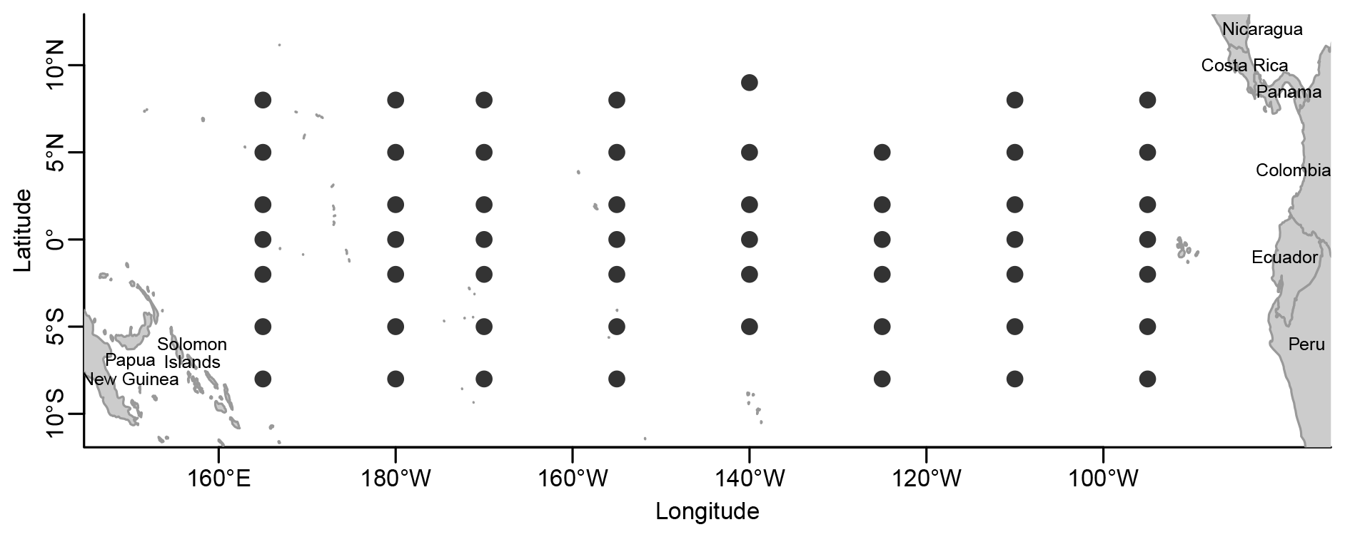
Figure 1 Locations of the 54 buoys in the current TAO array in the tropical Pacific.

One popularly used temperature anomaly is defined by removing seasonal averages over a given time period at each location. Thus, in addition to analyzing the raw difference series (SST minus MAT), we analyze seasonally adjusted difference series obtained by subtracting the average monthly differences over the entire period of 1996–2018 for both the buoys and ERA5.

In Sect. 2, we describe and illustrate the data and reanalysis used, while in Sect. 3 we present a statistical model for the different spatiotemporal difference datasets (buoy and ERA5; raw differences and seasonally adjusted differences) and describe our Bayesian inferences. The results appear in Sect. 4, and a discussion of our analysis is found in Sect. 5. The Supplement includes further data analyses and details of the model fitting procedure.

2 Data and exploratory data analyses

2.1 TAO buoy data

The TAO array of fixed ocean buoys in the tropical Pacific originated in 1984 (although some buoys were started earlier) as an effort to understand the El Niño phenomenon. The current array has 54 buoys, each measuring winds, sea surface temperature, relative humidity, air temperature, and subsurface temperature at 10 depths in the upper 500 m. We will focus on MAT (measured by a Rotronic MP-101A sensor for 2 min averages every 10 min) and SST (measured by a PMEL ATLAS module instantaneously six times an hour). A complete update and restructuring of the network is underway and is expected to be completed by 2027. A plot of the locations of the 54 buoys in the current TAO array is shown in Fig. 1.

The earliest measurement of both MAT and SST is from 7 March 1980 at the buoy at 110° W and the Equator. A summary of the data quality indicator for MAT and SST measurements is shown in Table S1 in the Supplement. We use data with quality classifications 1 (good), 2 (probably good), and 5 (adjusted). The quality is best if the sensor calibration agrees pre-deployment and post-deployment. If only one of the two calibrations is available, the quality is deemed probably good. The adjusted classification has used some data external to the sensor to adjust for pre- or post-calibration disagreement. Details about the arrays, their instrumentation, and their data quality control are given on the TAO website (Mangum et al., 1998).

We looked at patterns of missing data in the daily series at each location (Fig. S1 in the Supplement). At least part of the missingness is caused by the fact that buoys attract fish and therefore fishers, who purposely or inadvertently cut the wire holding the buoy in place (Connell et al., 2023). When buoys float away from their assigned location, a rescue ship is sent out to recover them. Another source of missing data was the 2012 decommissioning of a NOAA ship that had serviced the array since 1996 (McPhaden et al., 2023). Without mooring maintenance, the missingness rose to 70 %. The COVID restrictions also made it difficult to recover lost buoys, leading to higher missingness after 2019 (Boyer et al., 2023). Thus, we decided to only use data from 1996 to 2018.

The daily data are turned into monthly data by averaging data in months that have at least 15 d of non-missing data. (We average over the observed daily values within each month.) Figure S2 shows the resulting percentage of missing monthly values for the period 1996 to 2018. The percentage of missingness varies by location, ranging from 6 % (2° S, 140° W) to 51 % (2° N, 95° W).

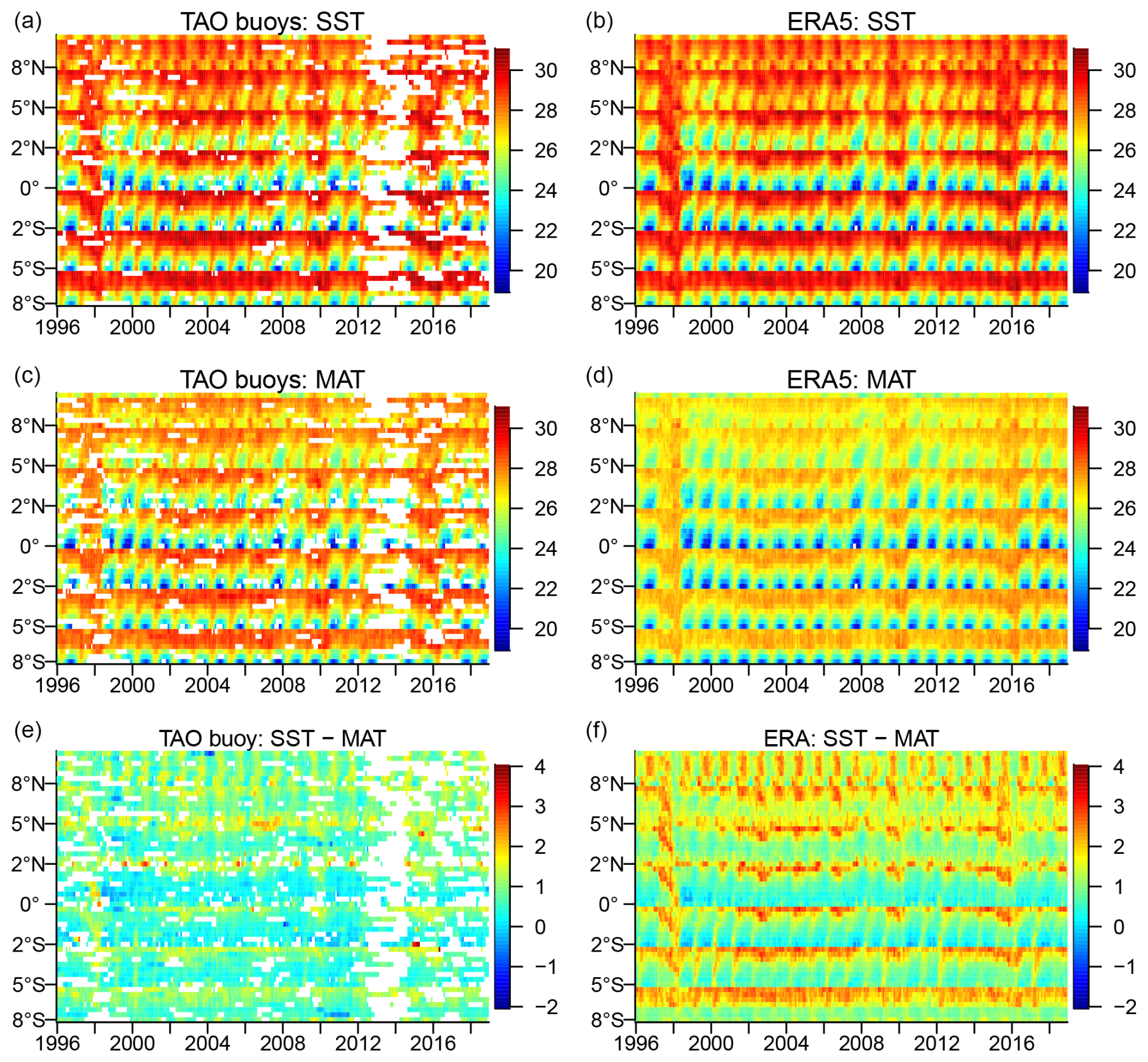
Figure 2 Heat maps of the SST, MAT, and their difference for the TAO buoy data (a, c, e) and the ERA5 data product (b, d, f). The units are degrees Celsius. In each panel the monthly time series by year (horizontal axis) are ordered from north to south and, within each latitude, from west to east (vertical axis).

2.2 Reanalysis data product

In order to get an alternative estimate of the SST and MAT, we go to the European Centre for Medium-Range Weather Forecasts' ERA5 (Hersbach et al., 2020). A reanalysis uses a current weather forecasting model of historical data. The input data for ERA5 come from satellites, weather balloons, weather data, buoys, ships, and other weather data. This is, however, not a coupled model. Rather, the sea surface temperature is prescribed using different Hadley Centre models (the OSTIA model since 2007), and the atmosphere is then run using the sea surface temperature as a boundary condition. ERA5 produces hourly data for a variety of variables on a 0.25° × 0.25° grid. We use the monthly means data products for SST and MAT, extracting 54 monthly time series of each variable at the grid cells closest to the locations of the TAO array of ocean buoys. There are no missing values for these 54 monthly SST and MAT series.

2.3 Exploratory data analysis

On average (over all of the buoys), the SST is about 0.76 °C warmer than the MAT at a monthly scale. The difference SST − MAT is directly proportional to the sensible heat flux (Cayan, 1980). Looking at the different buoy locations, the difference in the monthly means ranges from 0.21 (Equator and 125° W) to 1.55 (2° N and 95° W).

We show heat maps of the SST, MAT, and their difference (SST − MAT) for the TAO buoys in Fig. 2a, c, and e. Note the very sparse data availability around 2013. As expected, there are strong seasonal effects on the SST, MAT, and their difference that seem to vary by latitude and longitude over the tropical Pacific. The seasonal effects are stronger in the east, where the buoys are closer to the continental land, as compared to the west. While there are spatial variations in the average temperature over 1996–2018, it is hard to see long-term temporal trends.

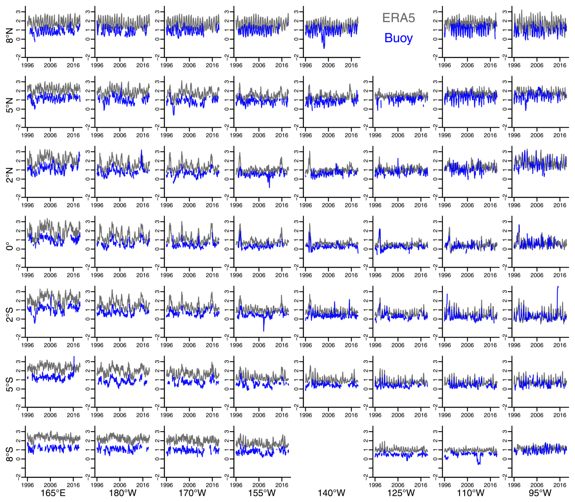
Figure 3 Buoy (blue) and ERA5 (gray) monthly differences (SST − MAT) for the 0.25° × 0.25° grid square containing the corresponding buoy location. This pictorial representation does not accurately represent the distances between the different buoy locations, and the series presented at 8° N and 140° W is actually at the location 9° N and 140° W.

Figure 3 shows, in blue, time series of observed differences between the sea surface temperatures and marine air temperatures for the TAO buoys. Each panel shows a different buoy location but does not accurately represent the distances between the locations (again, see Fig. 1 for the actual locations). While we observe seasonal variations that vary spatially in the difference SST − MAT, for the TAO buoys, the strength of these seasonal variations is weaker compared to examining the SST or MAT separately. This indicates that there is some agreement between the seasonal patterns for the sea surface and air temperatures in the tropical Pacific. Figure 3 indicates no evidence of long-term trends but some evidence that the average differences vary spatially for the buoys across this region.

2.3.1 Comparison to ERA5

We compare heat maps of the monthly SST, MAT, and SST − MAT for the TAO buoys (Fig. 2a, c, and e) and the ERA5 product (Fig. 2b, d, and f) in Fig. 2. Figure 3 shows for each buoy location the two time series of monthly TAO buoy differences and monthly ERA5 differences.

Clearly the ERA5 differences tend to be higher than the buoy differences, particularly in the western part. This could be because the forecast model in the version (CY41R2) of the ECMWF's Integrated Forecasting System used in ERA5 has a known cold bias in the lower regions of the troposphere over most parts of the globe (Haiden et al., 2021). Some outlying buoy patterns do not show up in ERA5 (e.g., 9° N, 140° W around 2004 and 2° S, 195° W around 2015). This may be due to unfortunate configurations of missing values.

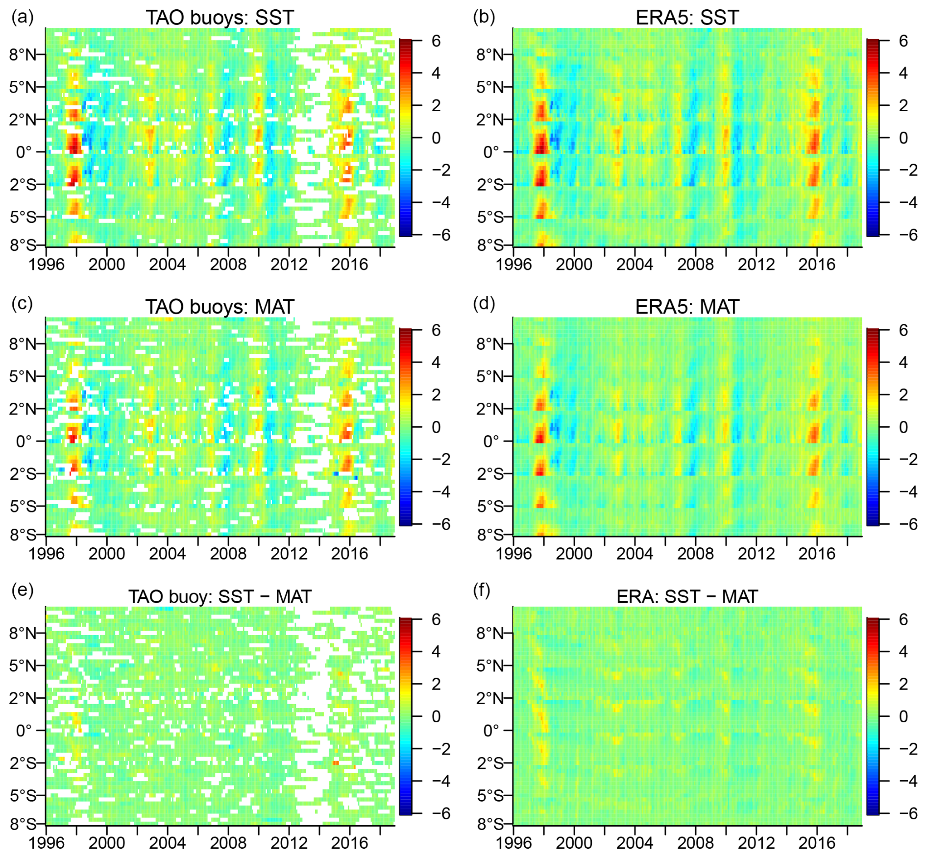
Figure 4 Heat maps of the seasonally adjusted monthly SST, MAT, and their differences for the TAO buoy data (a, c, and e) and the ERA5 product (b, d, and f). The units are degrees Celsius. In each panel the monthly time series by year (horizontal axis) are ordered from north to south and within each latitude from west to east (vertical axis).

As with the TAO buoy monthly SST, MAT, and their differences, we see strong seasonal variations in the corresponding monthly ERA5 series, varying spatially over the tropical Pacific (again, the seasonal effects are stronger to the west nearer the continental land). There is a suggestion that the seasonalities are not the same for the TAO buoys and ERA5 series, which we will examine further in our modeling efforts. Again, as with the TAO buoys, there is no visual evidence of long-term trends in the monthly differences for ERA5, but spatial variations in the average differences exist.

2.3.2 Seasonally adjusted monthly differences (anomalies)

The argument for using SST as a proxy for MAT in calculating global mean temperature is that the difference between the two does not change (on a global scale) over time (on a monthly scale), so when SST and MAT anomalies are calculated, the difference should be zero. We calculate anomalies by subtracting the longest possible monthly temporal average, in our case from 1996 to 2018. From now on we will call these anomalies seasonally adjusted monthly values.

Figure 4 shows the seasonally adjusted monthly values of the SST, MAT, and their difference. Making this seasonal adjustment takes care of the ERA5 cold bias in MAT and illustrates that the raw MAT from ERA5 should not be used as the ground truth for this measurement in the equatorial Pacific. Rather, ERA5 MAT seasonally adjusted monthly differences need to be used.

In the heat maps of seasonally adjusted monthly SST and MAT values, there are obvious warm and cold bands. They correspond to the Oceanic Niño Index (ONI), which essentially consists of temporally smoothed ocean temperature averages over the central region of the network. High values of the ONI correspond to high values of both SST and MAT. The index is closely related to the Southern Oscillation Index (SOI), which compares pressure gradients rather than temperature gradients. It is notable that this pattern is clearly discernible in the buoy data in spite of the substantial amount of missing data.

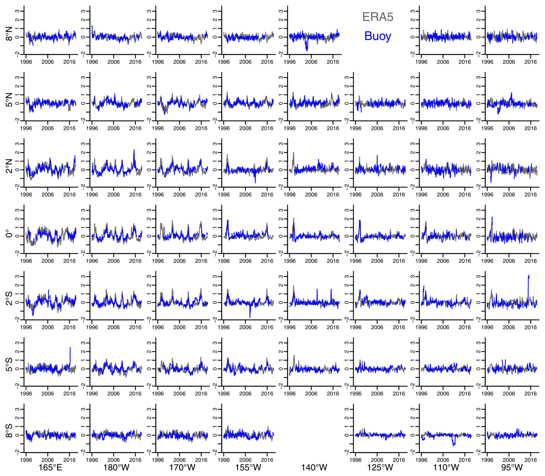
Figure 5 Buoy (blue) and ERA5 (gray) seasonally adjusted monthly differences for the 0.25° × 0.25° grid square containing the corresponding buoy location. This pictorial representation does not accurately represent the distances between the different buoy locations, and the series presented at 8° N, 140° W is actually at the location 9° N, 140° W.

Figure 5 compares the seasonally adjusted monthly differences calculated for the TAO buoys and the ERA5 product. We present this figure at the same vertical scale as Fig. 3. After seasonal adjustment, the TAO buoy and ERA5 differences are more similar, with little evidence of seasonality across the tropical Pacific. While there are local temporal disparities in the distributions of the seasonally adjusted monthly differences for the buoys and reanalysis product, the centers and spreads are similar at each spatial location. Together with the lack of visual evidence of long-term trends in these seasonally adjusted monthly differences, this suggests that, indeed, after seasonal adjustment, SST could be used in place of MAT. We next investigate this formally using statistical models for the differences.

3 Spatiotemporal modeling

In this section we introduce a hierarchical spatiotemporal model that we will fit to our four monthly difference datasets: the monthly differences, SST minus MAT, for the TAO buoy data; the monthly differences, SST minus MAT, for the ERA5 product; the seasonally adjusted monthly differences, SST minus MAT, for the TAO buoy data; and the seasonally adjusted monthly differences, SST minus MAT, for the ERA5 product. In the model below we refer to each dataset as the monthly differences. Again, our primary interest is to learn whether or not there are spatially varying temporal trends in each monthly difference dataset while accounting for possible spatially varying seasonal effects and residual spatiotemporal dependence.

Suppose that D⊂𝒮 is our continuous geospatial domain in the Pacific Ocean, where here 𝒮 denotes Earth's surface. Let T⊂ℤ denote the discrete-time index set. For a given dataset, we observe the monthly differences at m spatial locations in D denoted by ${\mathit{s}}_{\mathrm{1}},\mathrm{\dots },{\mathit{s}}_m$. At each spatial location s_j ($j=\mathrm{1},\mathrm{\dots },m$), let O_j⊂T denote the set of time indexes where we observe data. For the TAO buoy data, these indexes vary according to where we observe data at each location, whereas for the ERA5 product O_j=T for all j since there are no missing data. Then $\mathit{\left\{}Z\right({\mathit{s}}_j,t):j=\mathrm{1},\mathrm{\dots },m,t\in O_j\mathit{\}}$ denotes the observed spatiotemporal monthly differences for a given dataset.

Our interest is in modeling the underlying latent spatiotemporal difference process $\mathit{\left\{}Y\right(\mathit{s},t):\mathit{s}\in D,t\in T\mathit{\}}$. Assuming a standard Gaussian measurement error model, we assume that the observations are related to this latent process through

$$Z({\mathit{s}}_j,t)=Y({\mathit{s}}_j,t)+\mathit{ϵ}({\mathit{s}}_j,t),j=\mathrm{1},\mathrm{\dots },m,t\in O_j,$$

where we assume that $\mathit{\left\{}\mathit{ϵ}\right(\mathit{s},t):\mathit{s}\in D,t\in T\mathit{\}}$ is a mean zero Gaussian process that is independent over space and time. We suppose that the measurement error variance $\text{var}\left(\mathit{ϵ}\right(\mathit{s},t\left)\right)={\mathit{\sigma }}^{\mathrm{2}}>\mathrm{0}$ is constant over space and time.

Our model for the latent spatiotemporal difference process assumes that

$$Y(\mathit{s},t)=\mathit{\mu }(\mathit{s},t)+\mathit{\eta }(\mathit{s},t),\mathit{s}\in D,t\in T,$$

where $\mathit{\left\{}\mathit{\mu }\right(\mathit{s},t):\mathit{s}\in D,t\in T\mathit{\}}$ is the spatiotemporal mean process and $\mathit{\left\{}\mathit{\eta }\right(\mathit{s},t):\mathit{s}\in D,t\in T\mathit{\}}$ is a spatiotemporal irregular noise process that captures residual dependence not explained by the mean. Our spatiotemporal mean process can account for potential spatiotemporal trend components but also spatially varying seasonal-in-time components. Let $\mathit{\{}{x}_{k,t}:t\in T\mathit{\}}$, $k=\mathrm{1},\mathrm{\dots },K$ denote a set of K covariates that each vary over time. These covariates could be temporal trend covariates, or seasonal or periodic covariates. Then,

$$\mathit{\mu }(\mathit{s},t)=\sum _{k=\mathrm{1}}^K{\mathit{\beta }}_k\left(\mathit{s}\right)x_{k,t},\mathit{s}\in D,t\in T.$$

In our models for the TAO buoy and ERA5 monthly differences, we include an intercept, a linear trend term, and sine and cosine terms with periods of 1 year: thus, K=4. We find that using one sine term and one cosine term provides a reasonable and interpretable description for the periodicity observed in both the TAO buoy and ERA5 monthly differences. A less parsimonious description for the periodicity over years would mean including more sine and cosine terms with shorter periods, fitting a different term for each month, or using periodic splines (e.g., Perperoglou et al., 2019). With more complicated models we could use Bayesian model selection methods (e.g., Gelman et al., 2013, Sect. 7) to select between different models for the spatiotemporal mean process. In our models for the TAO buoy and ERA5 seasonally adjusted monthly differences, we include an intercept and a linear trend term but no sine or cosine terms. (Models for seasonally adjusted monthly differences that included yearly periodicities contained posterior seasonal components that were not different from zero.) We assume that the spatially varying coefficient processes $\mathit{\left\{}{\mathit{\beta }}_k\right(\mathit{s}):\mathit{s}\in D\mathit{\}}$ are a priori independent of k. For each k, $\mathit{\left\{}{\mathit{\beta }}_k\right(\mathit{s}):\mathit{s}\in D\mathit{\}}$ is a stationary Gaussian process with mean ${\mathit{\mu }}_{{\mathit{\beta }}_k}$ and covariance

$$\text{cov}\left({\mathit{\beta }}_k\right(\mathit{s}),{\mathit{\beta }}_k({\mathit{s}}^{\prime }\left)\right)={\mathit{\tau }}_{{\mathit{\beta }}_k}^{\mathrm{2}}\exp (-d(\mathit{s},{\mathit{s}}^{\prime })/{\mathit{\lambda }}_{{\mathit{\beta }}_k}),\mathit{s},{\mathit{s}}^{\prime }\in D,$$

where, for each k, ${\mathit{\tau }}_{{\mathit{\beta }}_k}^{\mathrm{2}}>\mathrm{0}$ is the variance parameter and ${\mathit{\lambda }}_{{\mathit{\beta }}_k}>\mathrm{0}$ is the spatial range parameter. Here, $d(\mathit{s},{\mathit{s}}^{\prime })$ denotes the chordal distance between the spatial locations s and s^′ in D. More specifically, writing these two spatial locations in terms of the longitude and latitude, i.e., $\mathit{s}=(\text{long},\text{lat}{)}^T$ and ${\mathit{s}}^{\prime }=({\text{long}}^{\prime },{\text{lat}}^{\prime }{)}^T$, we have

$$\begin{array}{rl}d(\mathit{s},{\mathit{s}}^{\prime })=& \mathrm{6.371}\left[\right(\cos \left(\text{long}\mathit{\kappa }\right)\cos \left(\text{lat}\mathit{\kappa }\right)\\ & -\cos \left({\text{long}}^{\prime }\mathit{\kappa }\right)\cos \left({\text{lat}}^{\prime }\mathit{\kappa }\right){)}^{\mathrm{2}}\\ & +\left(\cos \right(\text{lat}\mathit{\kappa }\left)\sin \right(\text{long}\mathit{\kappa })-\cos ({\text{lat}}^{\prime }\mathit{\kappa }\left)\sin \right({\text{long}}^{\prime }\mathit{\kappa }){)}^{\mathrm{2}}\\ & +\left(\sin \right(\text{long}\mathit{\kappa })-\sin ({\text{long}}^{\prime }\mathit{\kappa }){)}^{\mathrm{2}}{]}^{\mathrm{1}/\mathrm{2}},\end{array}$$

with $\mathit{\kappa }=\mathit{\pi }/\mathrm{180}$. The chordal distance is the Euclidean distance through a sphere with Earth radius 6.371 km, induces “a valid correlation function on the sphere” (Banerjee et al., 2004, p. 620), and ensures that the spatial range parameter is measured in thousands of kilometers.

We define our spatiotemporal irregular noise process $\mathit{\left\{}\mathit{\eta }\right(\mathit{s},t):\mathit{s}\in D,t\in T\mathit{\}}$ as follows. For t=1, let $\mathit{\eta }(\mathit{s},\mathrm{1})=\mathit{\zeta }(\mathit{s},\mathrm{1})$ for all s∈D. Then, for t≥2, let

$$\mathit{\eta }(\mathit{s},t)=\mathit{\varphi }\left(\mathit{s}\right)\mathit{\eta }(\mathit{s},t-\mathrm{1})+\mathit{\zeta }(\mathit{s},t),\mathit{s}\in D.$$

Thus, $\mathit{\left\{}\mathit{\eta }\right(\mathit{s},t):\mathit{s}\in D,t\in T\mathit{\}}$ is a spatiotemporal autoregressive process of order 1 – AR(1). In the above equation, $\mathit{\left\{}\mathit{\varphi }\right(\mathit{s}):\mathit{s}\in D\mathit{\}}$ is the spatially varying autoregressive parameter process and {ζ(s,t)} is a mean zero Gaussian spatiotemporal innovation process that is assumed to be independent over time but correlated over space. We model a transformation of the AR(1) parameter process $\mathit{\left\{}\mathit{\varphi }\right(\mathit{s}):\mathit{s}\in D\mathit{\}}$ to enforce stationarity in time: to guarantee that ϕ(s) lies in $(-\mathrm{1},\mathrm{1})$ for all spatial locations s∈D, we let

$$\mathit{\eta }\left(\mathit{s}\right)=\log \left(\right(\mathrm{1.0}+\mathit{\varphi }\left(\mathit{s}\right))/(\mathrm{1.0}-\mathit{\varphi }\left(\mathit{s}\right)\left)\right),\mathit{s}\in D,$$

and we assume that this transformed spatial process $\mathit{\left\{}\mathit{\eta }\right(\mathit{s}):\mathit{s}\in D\mathit{\}}$ is a stationary Gaussian spatial process with mean μ_η and covariance

$$\text{cov}\left(\mathit{\eta }\right(\mathit{s}),\mathit{\eta }({\mathit{s}}^{\prime }\left)\right)={\mathit{\tau }}_{\mathit{\eta }}^{\mathrm{2}}\exp (-d(\mathit{s},{\mathit{s}}^{\prime })/{\mathit{\lambda }}_{\mathit{\eta }}),$$

where ${\mathit{\tau }}_{\mathit{\eta }}^{\mathrm{2}}>\mathrm{0}$ is the variance parameter and λ_η>0 is the spatial range parameter. To enforce a stationary starting condition in time, for $\mathit{s},{\mathit{s}}^{\prime }\in D$, let

$$\text{cov}\left(\mathit{\zeta }\right(\mathit{s},t),\mathit{\zeta }({\mathit{s}}^{\prime },t\left)\right)=\left\{\begin{array}{ll}\frac{{\mathit{\tau }}_{\mathit{\zeta }}^{\mathrm{2}}\exp (-d(\mathit{s},{\mathit{s}}^{\prime })/{\mathit{\lambda }}_{\mathit{\zeta }})}{\mathrm{1}-\mathit{\varphi }\left(\mathit{s}\right)\mathit{\varphi }\left({\mathit{s}}^{\prime }\right)},& t=\mathrm{1};\\ {\mathit{\tau }}_{\mathit{\zeta }}^{\mathrm{2}}\exp (-d(\mathit{s},{\mathit{s}}^{\prime })/{\mathit{\lambda }}_{\mathit{\zeta }}),& \text{otherwise}.\end{array}\right.$$

In the above equation, ${\mathit{\tau }}_{\mathit{\zeta }}^{\mathrm{2}}>\mathrm{0}$ is the variance parameter and λ_ζ>0 is the spatial range parameter. Since $\mathit{\left\{}\mathit{\zeta }\right(\mathit{s},t):t\in T\mathit{\}}$ is stationary in time at each spatial location s∈D, the variance is constant over time with

$$\begin{array}{}\text{(1)}& \text{var}\left(\mathit{\zeta }\right(\mathit{s},t\left)\right)={\displaystyle \frac{{\mathit{\tau }}_{\mathit{\zeta }}^{\mathrm{2}}}{\mathrm{1}-{\mathit{\varphi }}^{\mathrm{2}}\left(\mathit{s}\right)}},t\in T.\end{array}$$

We fit our spatiotemporal models in the Bayesian paradigm, and thus we now discuss our specification of the prior distribution for the hyperparameters in the model. We assume that all of the hyperparameters are mutually independent. For the measurement error variance σ², we assume a prior that is an inverse Gamma distribution with shape 0.01 and rate 0.01. For parameters in the spatiotemporal irregular noise process $\mathit{\left\{}\mathit{\eta }\right(\mathit{s},t):\mathit{s}\in D,t\in T\mathit{\}}$, the variance ${\mathit{\tau }}_{\mathit{\zeta }}^{\mathrm{2}}$ has an inverse Gamma distribution with shape 0.01 and rate 0.01, and for the spatial range parameter λ_ζ we assume a weakly informative Gamma prior with shape 20 and rate 10. For the transformed AR(1) parameter process $\mathit{\left\{}\mathit{\eta }\right(\mathit{s}):\mathit{s}\in D\mathit{\}}$, we assume a normal distribution with mean 0 and variance 10 for the mean μ_η, an inverse Gamma distribution with shape 0.01 and rate 0.01 for the variance ${\mathit{\tau }}_{\mathit{\eta }}^{\mathrm{2}}$, and again a weakly informative Gamma prior with shape 20 and rate 10 for the range parameter λ_η. For each spatially varying coefficient process $\mathit{\left\{}{\mathit{\beta }}_k\right(\mathit{s}):\mathit{s}\in D\mathit{\}}$, for $k=\mathrm{1},\mathrm{\dots },K$, we also assume a normal distribution with mean 0 and variance 10 for the mean ${\mathit{\mu }}_{{\mathit{\beta }}_k}$, an inverse Gamma distribution with shape 0.01 and rate 0.01 for the variance ${\mathit{\tau }}_{{\mathit{\beta }}_k}^{\mathrm{2}}$, and again a weakly informative Gamma prior with shape 20 and rate 10 for the range parameter ${\mathit{\lambda }}_{{\mathit{\beta }}_k}$. The weakly informative priors for all of the spatial range parameters were constructed from spatial models of the parameter estimates obtained from site-by-site time series analyses of the monthly differences and monthly seasonally adjusted differences for both the TAO buoy data and the ERA5 product. We chose a single prior that was wide enough to capture the dependence observed for all of the different spatially varying parameters.

For each model, we draw samples from the posterior distribution of the parameters given the monthly differences using a Markov chain Monte Carlo (MCMC) algorithm that is summarized in Sect. S2 in the Supplement. After discarding the first 5000 samples, we draw 100 000 more samples from the posterior distribution, keeping every 10th sample. Running two independent MCMC algorithms, this yields 20 000 draws from the posterior of each model that we base our inference on. Trace plots of the two sets of MCMC samples and standard diagnostic calculations (e.g., Gelman et al., 2013, chap. 11) indicated good mixing of the Markov chains.

4 Results

4.1 Spatiotemporal models fit to the differences

We first fit our spatiotemporal model to the monthly differences (SST − MAT) for the TAO buoy dataset and the ERA5 product. (We consider models fitted to monthly de-seasonalized differences in the next subsection.)

Table 1 Posterior means with 95 % credible intervals in parentheses for hierarchical spatiotemporal Bayesian models fit to four different datasets. Each column shows the results for each dataset: (a) the monthly differences, SST − MAT, for TAO buoys; (b) the monthly differences, SST − MAT, for ERA5; (c) the seasonally adjusted monthly differences, SST − MAT, for TAO buoys; and (d) the seasonally adjusted monthly differences, SST − MAT, for ERA5.

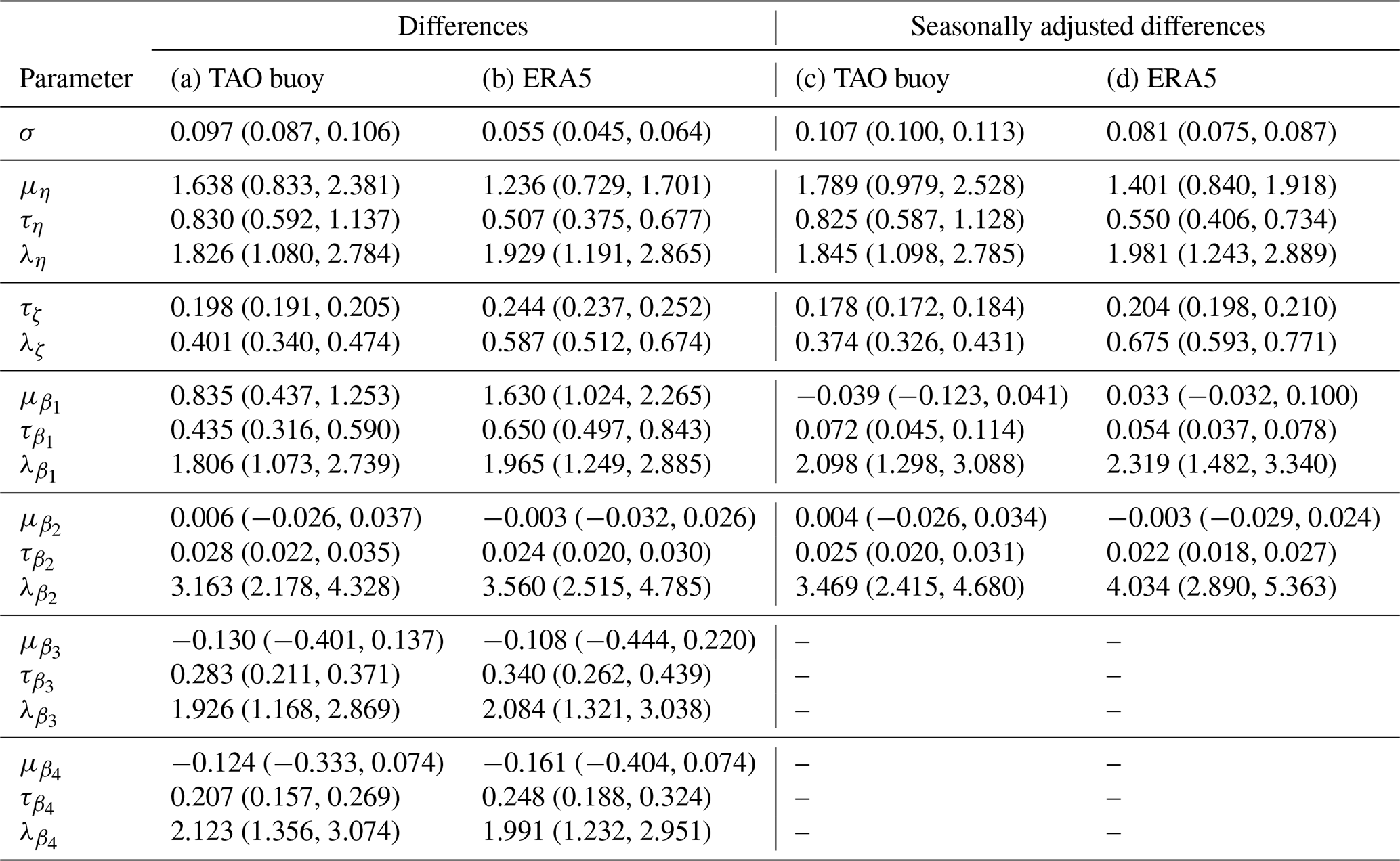
Column (a) of Table 1 presents summaries of the posterior distributions of hyperparameters in the model fit to the monthly differences for the buoys, while column (b) of the same table summarizes the posterior for the model fit to the monthly differences for ERA5. For each parameter, we calculate the posterior mean and show the 95 % posterior credible intervals in parentheses. Across most of the parameters, we find differences in the posterior distributions for the model fit to the buoys and the model fit to ERA5. For example, for the monthly differences, we learn that the measurement error standard deviation (SD), σ, is smaller for ERA5 than for the TAO buoys. This is to be expected as we anticipate that ERA5 will include more sources of information about the temperature in each grid box containing the TAO buoy location. Similarly, the mean for the intercept process, ${\mathit{\mu }}_{{\mathit{\beta }}_{\mathrm{1}}}$, is different from zero and positive for both datasets, indicating that the SST is higher than the MAT on average, but the difference is higher for ERA5 as compared to the buoys.

The SD parameters for the latent spatially varying processes (τ_η for the transformed AR(1) parameter process, τ_ζ for the spatiotemporal innovation process, and ${\mathit{\tau }}_{{\mathit{\beta }}_k}$ for the coefficient process with $k=\mathrm{1},\mathrm{\dots },\mathrm{4}$) all indicate that these processes have different uncertainties that need to be accounted for in both datasets. The range parameters for the latent spatially varying processes (λ_η, λ_ζ, and ${\mathit{\lambda }}_{{\mathit{\beta }}_k}$ for $k=\mathrm{1},\mathrm{\dots },\mathrm{4}$) are all different from one another. Even given the choice of an informative prior for these range parameters, there is some evidence of Bayesian learning relative to the prior, which assumes means of 2 and 0.025 and 0.975 quantiles of 1.222 and 2.967, respectively. Since a large range parameter indicates stronger spatial dependence, we learn that all latent processes exhibit stronger spatial dependence in the model fit to the ERA5 monthly differences as compared to the model fit to the buoy monthly differences. Looking across the different latent processes, the weakest spatial dependence occurs for the spatiotemporal innovation process, as measured by λ_ζ, whereas the strongest spatial dependence occurs for the coefficient process for the spatially varying linear trend, as measured by ${\mathit{\lambda }}_{{\mathit{\beta }}_{\mathrm{2}}}$.

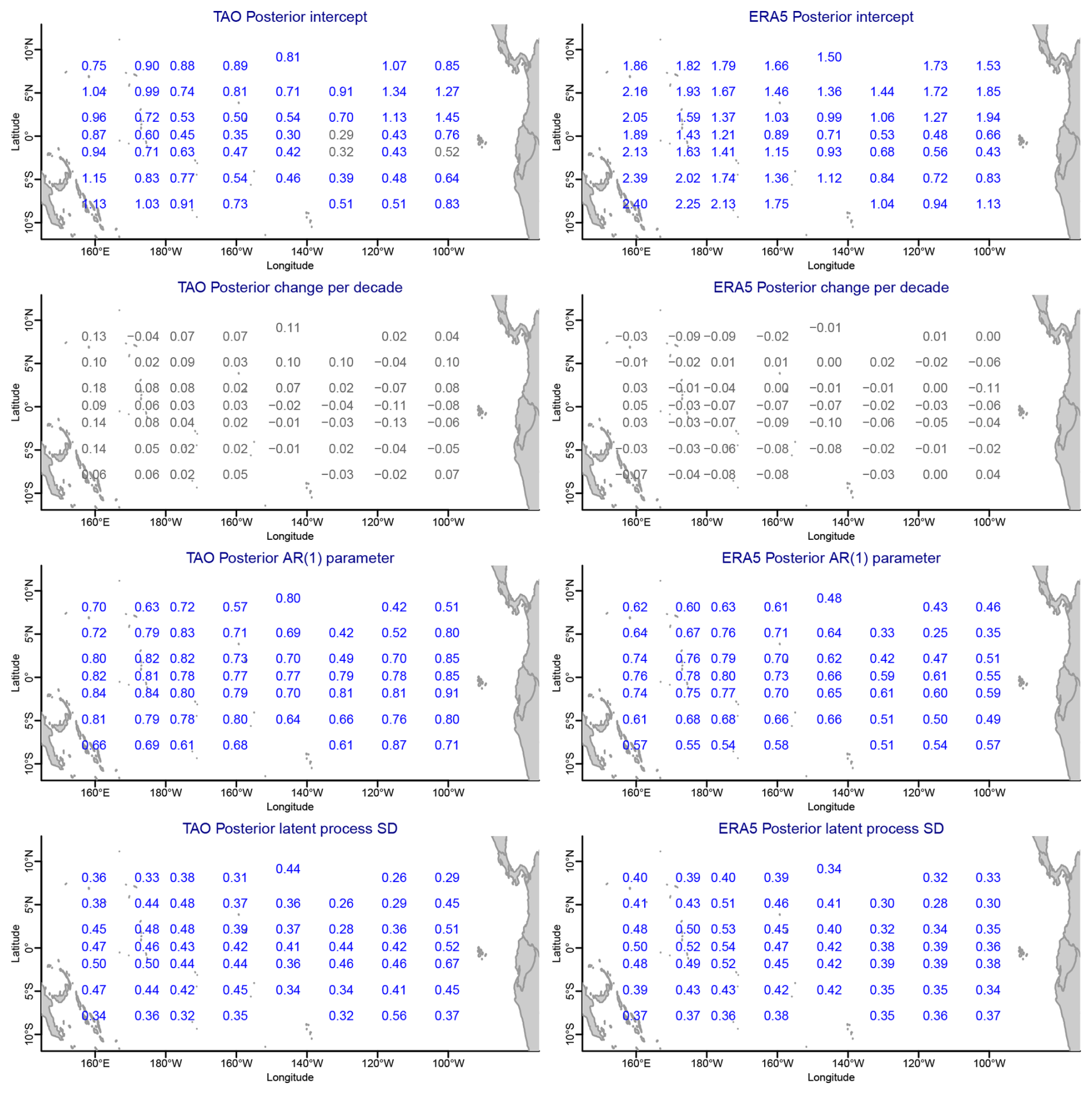
Figure 6 A summary of the spatially varying posteriors from the hierarchical spatiotemporal Bayesian models fit to the monthly differences SST − MAT for the TAO buoys (first column) and ERA5 (second column). The values are the posterior means for the spatially varying intercepts (first row), the spatially varying decadal trend (second row), the spatially varying AR(1) parameters (third row), and the spatially varying process standard deviations (fourth row). The gray values indicate that the simultaneous 95 % credible interval for the parameter at that location contains zero, whereas the blue values indicate that the interval does not contain zero.

Figure 6 displays posterior summaries of the spatially varying parameters in each of the two models: the first column shows the posterior means for the model fit to the monthly differences for the TAO buoys, and the second column shows the posterior means for the model fit to the monthly differences for ERA5. In the different rows we present different parameters: posterior means for the spatially varying intercepts (first row), the spatially varying decadal trends (second row), the spatially varying AR(1) parameters (third row), and the spatially varying AR(1) process SDs calculated using the square root of Eq. (1) (fourth row). For each panel we calculate simultaneous 95 % credible intervals for the parameters over the different locations using the simconf.mc function from the excursions R package (Bolin and Lindgren, 2017, 2018). If the interval at each location contains zero, we present the posterior mean at a given location in gray, indicating that there is no evidence that the parameter at that location is not zero, suitably accounting for multiple comparisons. If the posterior mean is shown in blue, however, there is evidence that the parameter at that location is not zero.

Examining the second row of Fig. 6, we see that, over the tropical Pacific, all slopes measured by change per decade in the models for the buoy and ERA monthly differences are not different than zero. This indicates no evidence of linear trends in the difference, SST − MAT, on a monthly timescale. However, we see that most intercepts in the models for the buoy and ERA monthly difference models (the first row) are greater than zero. Thus, both the buoy and ERA5 datasets indicate that the sea surface temperature, SST, is higher than the marine air temperature, MAT, at most of the locations. This difference varies by location and dataset. Expanding on our earlier exploratory analysis, SST is significantly higher than MAT in the ERA5 dataset as compared to the TAO buoy network. This indicates that, on the monthly timescale without de-seasonalization, the average monthly SST values are not interchangeable with the average monthly MAT values, regardless of the dataset that we use.

The third row of Fig. 6 compares the spatially varying AR(1) parameter, which measures the strength of temporal dependence in the latent monthly difference process estimated for the TAO buoys (left column) and ERA5 (right column). The fourth row of the same figure indicates the spatially varying AR(1) process SDs, again calculated from the square root of Eq. (1). From these panels, we learn that there is significant temporal dependence over all locations in the tropical Pacific, which again varies over the region of interest. The temporal dependence estimated from ERA5 tends to be weaker than that from the TAO buoys, which suggests that the ERA5 product, which includes more sources of information about the SST and MAT, introduces less temporal dependence at a monthly scale than the TAO buoy network values. While there are differences in the process SDs over the region, the values for the buoys and ERA5 are more similar.

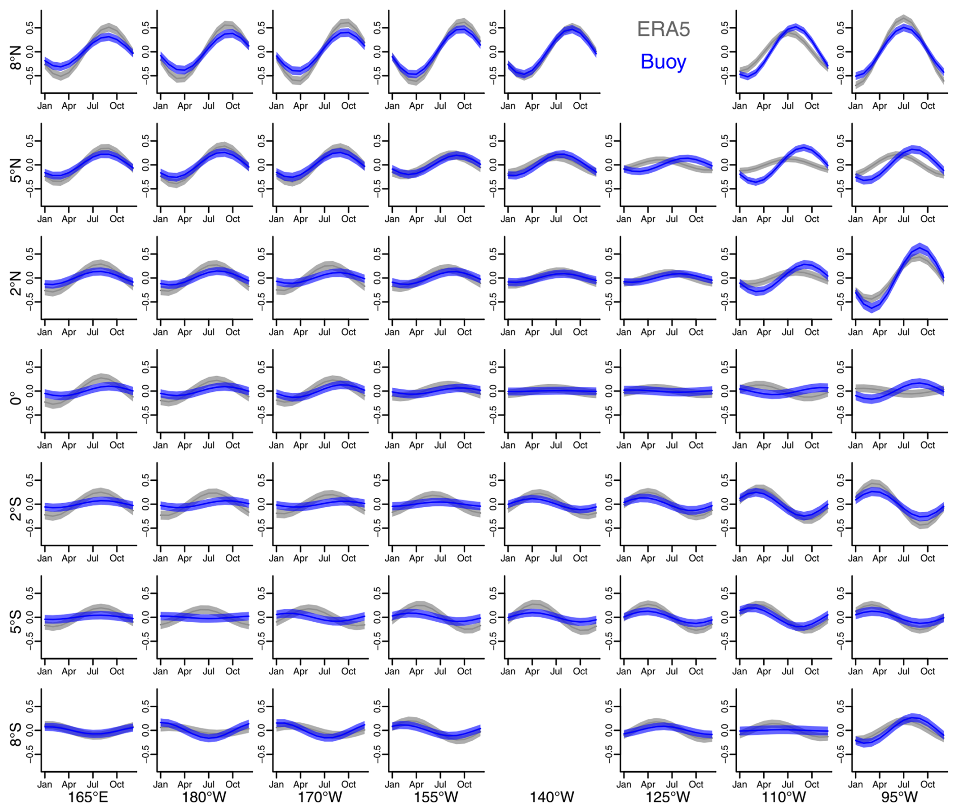
Figure 7 Posterior summaries of the seasonal terms from hierarchical spatiotemporal Bayesian models fit to the differences, SST − MAT, for TAO buoys (blue) and ERA5 (gray), as a function of longitude and latitude. For each seasonal term, the solid dark lines indicate the posterior mean as a function of the month, and the lighter-shaded regions denote 95 % simultaneous credible intervals. This pictorial representation does not accurately represent the distances between the different buoy locations, and the series presented at 8° N and 140° W is actually at the location 9° N and 140° W.

Figure 7 compares the posterior distribution of the spatially varying seasonal components estimated for the monthly differences of the buoys (in blue) and ERA5 (in gray) for the different locations in the tropical Pacific. In each panel the solid line shows the posterior mean value estimated for each month, and the shaded regions indicate simultaneous 95 % credible intervals, again estimated using the methods of Bolin and Lindgren (2017, 2018). These figures indicate a spatial variation in the seasonalities that varies by the dataset used (buoy or ERA5). As a reminder, each seasonality is a summary of the seasonal variation in the monthly differences SST − MAT, not the seasonalities of SST and MAT. We would expect stronger seasonalities in SST and MAT as we move away from the Equator, but we expect the seasonal structure of the differences to be less pronounced. For the differences we also see stronger seasonal structures as we move away from the Equator and closer to the continental land in the east (there are only islands to the west of the region of interest in the tropical Pacific). Different seasonalities for the monthly differences indicate that the yearly seasonal structures of SST are different from the yearly seasonal structures of MAT and further point to the fact that SST and MAT are not interchangeable on the raw monthly scale in the tropical Pacific.

4.2 Spatiotemporal models fit to the seasonally adjusted differences

Next, we fit our spatiotemporal model to the monthly seasonally adjusted differences (SST − MAT) for the TAO buoy dataset and the ERA5 product. Since we have already de-seasonalized the values in each dataset, in these models we do not include seasonality terms that vary over the spatial locations. (As mentioned earlier, we verified this assumption by examining a more complicated model which included yearly seasonality terms.) However, we still include a constant and linear trend term at each location, which can vary spatially over the tropical Pacific.

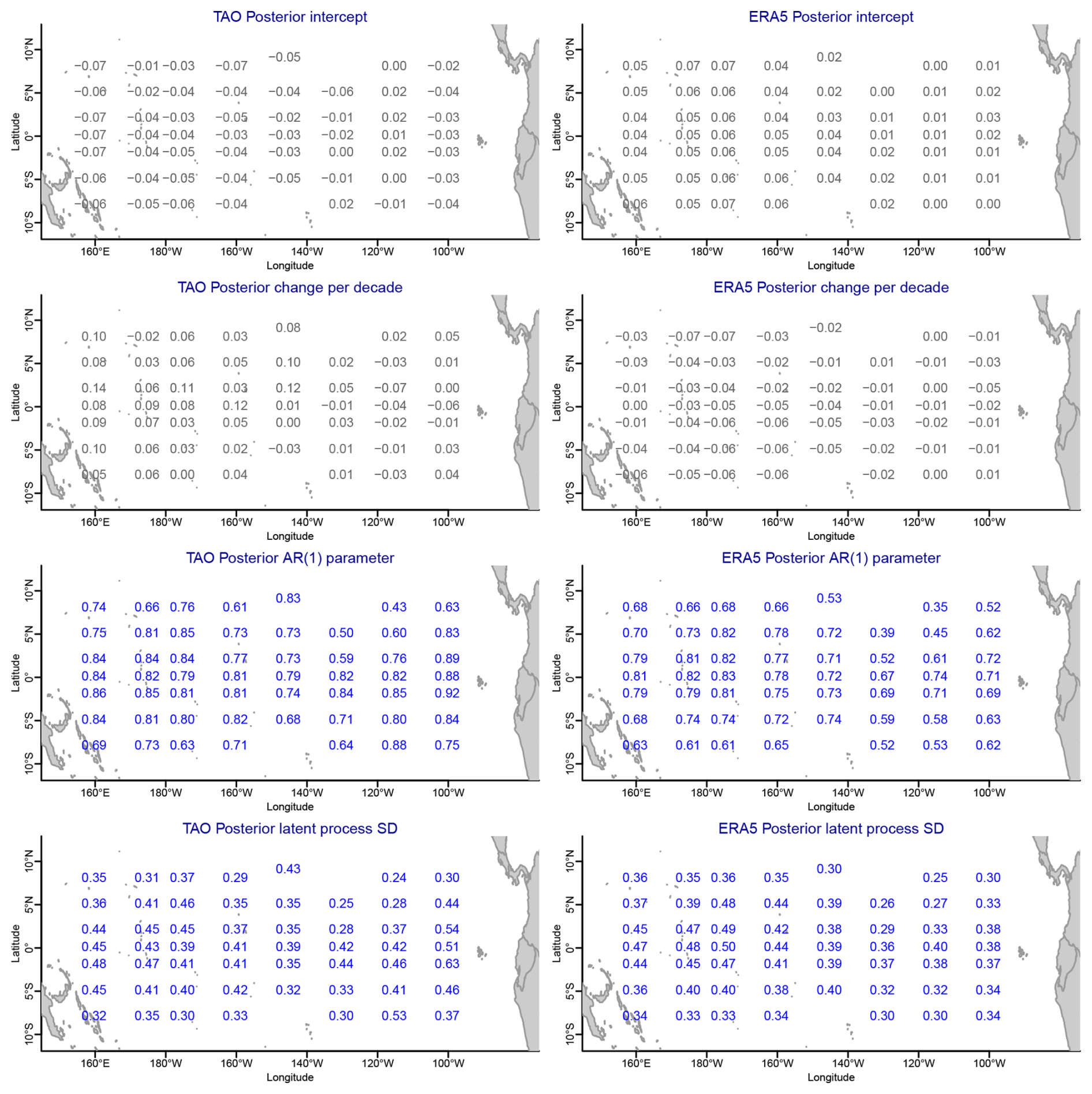
Figure 8 A summary of the spatially varying posteriors from the hierarchical spatiotemporal Bayesian models fit to the seasonally adjusted monthly differences, SST − MAT, for the TAO buoys (first column) and ERA5 (second column). The values are the posterior means for the spatially varying intercepts (first row), the spatially varying decadal trend (second row), the spatially varying AR(1) parameters (third row), and the spatially varying process standard deviations (fourth row). The gray values indicate that the simultaneous 95 % credible intervals for the parameter at that location contain zero, whereas the blue values indicate that the interval does not contain zero.

Column (c) of Table 1 presents summaries of the posterior distributions of hyperparameters in the model fit to the monthly seasonally adjusted differences for the buoys, while column (d) of the same table summarizes the posterior distributions for the model fit to the monthly seasonally adjusted differences for ERA5. Comparing the model fit to the monthly (not seasonally adjusted) differences, we learn that the process parameter for the measurement error SD (σ) is similar for the buoys but larger for ERA5. The parameters for the spatially varying AR(1) parameters (μ_η, τ_η, and λ_η) and the spatiotemporal innovation process (τ_ζ and λ_ζ) vary little in either model fit to the seasonally adjusted monthly differences as compared to the model fit to the monthly differences. This suggests that these spatial characteristics do not vary after seasonal adjustment.

After seasonal adjustment, both intercept terms (as measured by ${\mathit{\mu }}_{{\mathit{\beta }}_{\mathrm{1}}}$ for the buoys and ERA5) are now not different from zero and have a smaller SD compared to the models fit to the datasets without seasonal adjustment (as measured by ${\mathit{\tau }}_{{\mathit{\beta }}_{\mathrm{1}}}$). Figure 8 displays posterior summaries of the spatially varying parameters in each of the two models fit to the seasonally adjusted monthly differences. This plot is arranged similarly to Fig. 6. The first row of Fig. 8 indeed confirms that, once we seasonally adjust SST and MAT, we cannot tell their difference apart on average (the posterior intercepts at the different locations for both the buoy and ERA5 spatiotemporal models are not different from zero). Likewise, the second row of Fig. 8 indicates no evidence that SST − MAT has linear trends at any location in the region of interest, once we seasonally adjust it. While the spatially varying AR(1) parameters and process SDs vary a little for the seasonally adjusted models compared to the non-seasonally adjusted models, there is little evidence that the spatiotemporal dependence characteristics have changed.

5 Summary and discussion

In this article we study the difference between sea surface temperature (SST) and marine air temperature (MAT) over the tropical Pacific, using data from the TAO buoys. As is well known, SST is typically warmer than MAT, but when using seasonally adjusted differences as our anomaly, there is no substantial difference. Our spatiotemporal models indicate no significant temporal trends at the locations of the TAO buoys for both the TAO buoy monthly differences and seasonally adjusted monthly differences as well as the ERA5 monthly differences and seasonally adjusted monthly differences, disagreeing somewhat with the findings of Rubino et al. (2020). The main difference from that work is that we are able to fit linear trends for each station over the entire time period, regardless of the missing value pattern. Rubino et al. (2020) found occasional short-term non-significant ordinary least-squares (OLS) trend differences between SST and MAT anomalies.

Comparing the seasonally adjusted monthly difference buoy data to the corresponding grid square values from the ERA5 seasonally adjusted monthly differences, we see no major difference between the two datasets using our spatiotemporal models. Thus, our results indicate that SST and MAT are interchangeable for computing global seasonally adjusted monthly temperature anomalies in the tropical Pacific. In order to extend these findings to the globe, we could analyze a coupled reanalysis, where there is a realistic interaction between sea surface and marine air temperatures. This would also have been the preferred reanalysis for this study. Unfortunately, we have not found any coupled reanalysis that covers the time period of our study.

We have chosen to use statistical tools that allow us to estimate and predict the missing values in our spatiotemporal model. This allows us to fully account for all uncertainty in the TAO buoy values. However, one could have imputed these missing data values before fitting a statistical model. There are a variety of ways to do this. A blending approach replaces missing values with the corresponding ERA5 values. Due to the bias in ERA5 MAT, this can only be done using the monthly seasonally adjusted values. Another approach, due to Fuentes et al. (2006), is to compute a singular value decomposition (SVD) of the space–time data matrix, iterating between computing the SVD for the matrix and replacing the missing values by linear regression of the columns onto the first SVD component. As an initial replacement for the missing values, regression on the column averages is used. This function is implemented as SVDMiss in the SpatioTemporal R package available in the CRAN archive.

To understand the robustness of our results to missing data, we imposed the same missing data pattern as for the buoys on the ERA5 data and refit our model to this dataset. Other than an increase in the uncertainty in estimating parameters in the spatiotemporal model fit to this dataset as compared to the model fit to the ERA5 data with no missingness imposed, no other appreciable disparities could be detected. This indicates that no bias was induced by the missingness observed in the TAO buoy network. Given the extent of the missingness in the TAO buoy network, we were also worried that there could be an association between missingness and the temperature values themselves. Such a phenomenon is known as preferential sampling (e.g., Diggle et al., 2010; Gelfand et al., 2012). Exploratory plots comparing the SSTs and MATs to summaries of the missing data pattern indicated no evidence of preferential sampling. Additionally, we note that the comparison of point measurements (TAO buoy values) to grid square predictions (the ERA5 product) is not ideal. One could either downscale the ERA5 data to the point locations given by the observational network or upscale the point locations to grid squares (e.g., Berrocal et al., 2012). However, each of these options would require substantial additional modeling and computer processing.

Our latent space–time difference process assumed an autoregressive model of order 1 in time at each location, with a temporal dependence that varies by location and a spatiotemporal innovation process that is independent over time but correlated in space. This gave a good summary of the observed dependence. More complicated models with more involved dependence structures may better account for uncertainty in the monthly differences but would be computationally more challenging to fit. Likewise, we used exponential spatial covariance functions throughout to capture the spatial dependence in various parts of the model, ranging from the latent space–time difference process but also the spatially varying parameter processes. While there is an advantage in allowing the degree of smoothness of the spatial processes to change by using more general covariance functions such as the Matèrn covariance function (e.g., Stein, 2012), the gridded nature of the TAO buoy measurements and ERA5 data product limits our ability to accurately estimate any smoothness parameter. Also, as is often the case, there was some difficulty estimating the range parameters for the spatial correlations using relatively uninformed priors. We therefore chose informative priors that allowed some learning; i.e., the posterior density was not the same as the prior density. Slight changes to the form of the prior for the range parameters do change the results slightly, given the dependence between the posterior distributions for the mean, variance, and range parameters of the spatial processes. Another approach might be, rather than to impose independent priors, to assign multivariate spatial priors within contiguous blocks of buoy sites with independence only between blocks, thereby enforcing some spatial dependence even in the priors.