the Creative Commons Attribution 4.0 License.
the Creative Commons Attribution 4.0 License.
 | 05 Sep 2025
A new data-standardization procedure for comprehensive outlier detection in correlated meteorological sensor data
Temesgen Zewotir
Rajen N. Naidoo
Delia North
Studies that investigate the effects of meteorological fluctuations on varying multi-disciplinary outcomes often depend on analysis of high-frequency sensor data from automatic monitoring stations in different locations. The validation of such spatial time series requires attention given that they are susceptible to multiple forms of error. Existing validation techniques tend to cater to detection of only one form of outlier in isolation, lack robustness, or fail to optimally leverage the strong between-series correlation that often prevails in high-frequency meteorological data exhibiting multiple seasonalities. To address these shortcomings, two adaptations were made to an existing procedure, for more powerful outlier detection in strongly correlated high-frequency time series, using a distributional approach. The modified technique was tested in a simulation study and was also applied to a real univariate spatial set of hourly air temperature series from the South African Air Quality Information System. In both instances, the effectiveness of the technique in detecting outliers was assessed relative to procedures lacking either or both adaptations. The results show the modified procedure to be most comprehensive in the simultaneous detection of multiple forms of error, including solitary spikes, shifts in the series mean, and irregularities in the diurnal pattern. Furthermore, the method is generalizable to any set of time series displaying a similar correlation structure.
- Article
(1510 KB) - Full-text XML
- BibTeX
- EndNote


The ambient measurement of meteorological variables at high frequency, via automated sensors, serves many purposes that extend beyond weather surveillance. In particular, studies that investigate the effects of meteorological fluctuations on varying multi-disciplinary outcomes often rely upon the analysis of ground-level monitoring data, either directly or indirectly, for the adjustment of models developed using covariate data derived from satellite imagery (Moreno-Tejera et al., 2015). Such high-frequency time series are usually collected, processed, and transmitted by automatic monitoring stations (AMSs) situated in different locations. A wide range of meteorological variables may be measured as often as every few minutes over an extended period, with the resulting data series thus being characterized by multiple forms of seasonality. For example, the values of hourly surface air temperature readings will depend not only on the hour of the day but also on the month (or week) of the year in which they are recorded.
Due to the predictable 24 h rotation of the Earth, many meteorological variables respectively exhibit a very strong positive linear correlation over time between differing spatial locations when measured at high frequencies (e.g. air temperature, atmospheric pressure, solar radiation, and humidity). This is provided that the measurement locations are close enough to one another (no more than 200 km apart) to be subject to the same intermediate mesoscale weather systems (Penn State Department of Meteorology, 2025). However, in general, the quality of data that are recorded near-continuously by programmed reading instruments in the absence of direct regular human observation tends to be extremely poor and is often marred simultaneously by numerous varying forms of error or outliers (Schlüter and Kresoja, 2020). This can result in the observed temporal correlations between univariate series within a spatial set being artificially lower than they typically would be if the data were perfectly clean.
In this article, we distinguish between differing forms of outlier by referring to single outliers and to multiple consecutive or sequential outliers. Both forms of outlier mentioned often arise in automated high-frequency meteorological data recorded at ground level – due either to the use of a lower-cost apparatus having been distributed at high density (Van Poppel et al., 2023), because of changeovers in the system, or human error in the programming of higher-grade systems (Schlüter and Kresoja, 2020). A single outlier is typically observed as a solitary spike or dip in the data. A consecutive sequence of outliers may present itself either as a level shift (increase or decrease in the series mean) or as an irregularity in the seasonal (usually diurnal) pattern. Irregular patterns are the most difficult to identify (Schlüter and Kresoja, 2020), as they present themselves in the form of sub-sequences that are only improbable during certain parts of the diurnal cycle.
The literature highlights that existing outlier detection methods for time series are sub-optimal for the type of high-frequency, error-prone meteorological data described above. Our appraisal of published works highlights that current techniques fail to optimally leverage the strong between-series correlation that often prevails in high-frequency meteorological data. Furthermore, they frequently lack robustness when applied to data sets containing extreme or extensive error, and they tend to cater to the detection of only one form of outlier in isolation.
For example, based on their extensive review, Blazquez-Garcia et al. (2021) conclude that there is a need for validation techniques which leverage more fully the temporal correlation between time series within a spatial or multivariate set and which further make contingency for every series within the set to be equally likely to contain outliers. This would be contrary to applying the distorted but common assumption that particular series within the set may be regarded as clean and used as a reliable benchmark. In their review, Blazquez-Garcia et al. (2021) also provide a structured classification of existing methods in which they distinguish between them, predominantly according to the type of outlier that each has been designed to detect (solitary versus multiple sequential). Similarly, Posio et al. (2008) discuss the pros and cons of a wide variety of outlier detection methods and suggest that, in order for the choice of technique to be optimal, prior knowledge is needed of the type of inconsistencies likely to be present in the data. Schlüter and Kresoja (2020) determine their “autoregressive cost update mechanism” to be more effective at identifying solitary outliers, whereas their “wavelet-based mechanism” is deemed more effective at detecting the presence of multiple consecutive outliers. They advocate for the implementation of a combination of data pre-processing tools in order to ensure a comprehensive approach to outlier detection.
Since prior knowledge may not exist of the outlier type or types present within a time series – particularly those retrieved using an automated sensor – the literature infers that several existing validation techniques would need to be employed in order to ensure comprehensive detection of both solitary and sequential outliers within sensor-dependent meteorological data. Clearly this is undesirable, with a need for the development of a single deft solution. For high-frequency univariate spatial time series in particular, the type of seasonality present within the data also demands consideration in the detection of outliers as well as the strength of the temporal correlation between series.
In this paper, we present a new method for standardizing meteorological sensor data, with the purpose of enabling comprehensive detection of multiple varying forms of outlier in strongly correlated series that typically come from high-frequency measurements being collected across different locations. In Sect. 2, we provide a detailed discussion of the limitations and weaknesses of existing validation procedures for correlated series. In particular, we draw attention to a parsimonious method which employs, twice over, a conventional data-standardization approach to outlier detection but which is best-suited for the validation of lower-frequency, more moderately correlated data. In Sect. 3, we formulate a new procedure for detecting outliers in high-frequency, strongly correlated series by making two adaptations to the double-standardization procedure described in Sect. 2. Whilst still preserving the simplicity of the original double-standardization procedure, we take into account the presence of multiple seasonalities within high-frequency data so that we are able to fully leverage the between-series correlation structure. Furthermore, we introduce the use of robust statistics into the standardization of the data to ensure sensitivity of detection. In Sect. 4, we design and conduct a Monte Carlo simulation study to test the effectiveness of the new procedure in the simultaneous detection of multiple varying forms of outlier within strongly correlated simulated series. We assess performance relative to double-standardization procedures lacking either or both procedural adaptations. We show the modified technique to be more reliable in the simultaneous detection of varying forms of moderate and severe outliers. In Sect. 5, we present a case study in which we apply the new validation procedure to an actual data set containing an unknown element of error. We similarly find the modified technique to be highly sensitive and more comprehensive in the simultaneous detection of varying forms of outlier than other comparable double-standardization procedures. In Sect. 6, we summarize our conclusions and suggest possible avenues for extension in future work.
Many existing methods for the detection of outliers in multivariate time series do attempt to account for the temporal correlation that is commonly present between different variables in order to avoid “loss of information” (Blazquez-Garcia et al., 2021). Such techniques reduce the dimension of the data to a single variable or a reduced set of uncorrelated variables, to which univariate methods of outlier detection are then applied. A similar approach might be applied to validate the correlated univariate spatial time series that arise when the same weather variable is concurrently measured across a number of different locations at high frequency, with the series displaying largely parallel trends over time. However, this would only serve to detect outliers that simultaneously affect multiple time series (Blazquez-Garcia et al., 2021). The presence of outliers that occur independently within a given series would be overlooked.
One approach to validating seasonal, univariate spatial time series that caters to the possibility of independent outliers within each series and also attempts to account for temporal correlation between series is a double-standardization procedure employed by Washington (2020) for the validation of a spatial set of daily maximum temperature series spanning several years. The method draws on the work of Lund et al. (1995) as well as a technique titled “climatologically aided interpolation” that was proposed by Willmott and Robeson (1995). The procedure adopts, twice over, a conventional “z-score” approach to outlier detection (Moore et al., 2009) whilst controlling overtly for seasonality within each series.
As Moore et al. (2009) explain, z scores are generally derived by leveraging the distribution of the data to apply the following transformation:
where x denotes the original data value, μ=mean(x), and σ = standard deviation(x).
As a first step in the data-validation procedure employed by Washington (2020), each series is independently standardized by replacing the original data values with their corresponding z scores, but the z scores are derived using seasonally controlled parameter estimates for the mean and the variance. For example, Washington opts to standardize each of the daily maximum temperatures recorded in the month of February, using the mean and standard deviation of all daily maximum temperatures recorded in the month of February across different years. Each of the daily maximum temperatures recorded in the month of March is transformed using the mean and standard deviation of all daily maximum temperatures recorded in the month of March, and so on. This seasonally controlled approach to preliminarily (and independently) standardizing every time series within the spatial set permits separate initial flagging of potential outliers within each series through inspection of how many standard deviations above or below the relevant seasonal mean each value lies and through application of a threshold.
In the next step of Washington's procedure, each of the z scores is subsequently standardized but this time using the spatial distribution of the z scores across series (locations) at each time point (or rolling window of time) within the data set. For example, if we consider, say, 13 February 1984 to be one particular time point within Washington's daily spatio-temporal data set, each of the z scores from across the differing locations within the spatial set, relating to that particular date only, is standardized using the mean and standard deviation of all z scores relating to that date (or narrow window of time around that date) across series. This subsequent round of standardization in Washington's procedure enables secondary confirmation of whether each data point that was preliminarily flagged as an outlier (after step 1) should remain as such, based on how many standard deviations the corresponding z score lies above or below the mean of the z scores across series observed within a narrow window around the relevant time point.
The double-standardization procedure described above is conceptually designed to address the following sequential questions:
-
Is each reading at a “normal” level for the given location in the given seasonal period?
-
For those that are not, is each abnormally high or low reading in fact normal in relation to the mean reading being recorded at all of the locations, within a narrow window around that same respective time point?
This procedure was proposed, most sensibly, for the validation of a moderately correlated set of univariate spatial time series, thus necessitating that outlier detection rely primarily on independent detection within each series alone and less so on leveraging correlation dependencies. Furthermore, the procedure was applied to daily data exhibiting only one type of seasonality, with temperature values being treated as dependent on the month of the year (rather than the week of the year). Thus, the prevailing between-series correlation structure was largely retained in the standardized data set after step 1 of the procedure, despite controlling for season (month) during the preliminary transformation of each series. This is due to the fact that, for the most part, consecutive data points within a given series were standardized using the same distributional parameters (mean and standard deviation), with the only exceptions occurring at change points in a month. For example, a daily maximum temperature recorded on, say, 31 March was standardized using a different set of distributional parameters to the next daily maximum temperature recorded on 1 April. However, each of the daily maximum temperatures recorded sequentially from 1 to 31 March was standardized using the same set of distributional parameters, and so the change in the resulting z scores from one day to the next – relative to the standard deviation of the data – was the same as the corresponding change in the original data values. Thus, in the context of daily spatial time series, the extent to which differing pairs of series change together is largely preserved in the standardized version of the data, and hence so too is the between-series temporal correlation, even when the preliminary standardization of each series is performed by overtly controlling for seasonality.
In contrast, if the double-standardization procedure described above were to be applied to a higher-frequency time series of hourly air temperature readings that extend over several months and thus exhibit multiple seasonalities (including both the hour of the day with a periodicity of 24 and the month of the year with a periodicity of 12), then the between-series correlation structure would not be retained. In this scenario, each consecutive data value within a given series would be standardized using a different set of distributional parameters. For example, within a given series, each temperature reading recorded at a time of, say, 01:00 LT on any given day in, say, February would need to be transformed using the mean and standard deviation of all temperature readings in that series recorded at a time of 01:00 LT in the month of February. However, subsequent readings recorded at a time of 02:00 LT would need to be transformed using the mean and standard deviation of all temperature readings recorded at a time of 02:00 LT in the month of February. Hence, the change in the resulting z scores from one hour to the next – relative to the standard deviation of the data – would differ from the corresponding movement in the original data series. The benefit of subsequently standardizing the z scores across series (locations) using their spatial distribution at each time point would then be limited given that seasonally controlled series standardization of hourly data (exhibiting multiple seasonalities) decreases the prevailing temporal correlation between series. We later provide evidence to corroborate this in Sect. 4.
Moreover, for the type of high-frequency error-prone sensor data considered in this paper, the other weakness of the double-standardization procedure described above is that the sensitivity of the outlier detection would be inhibited by the widely acknowledged susceptibility of z scores to bias. When robust estimates are not used for the mean and standard deviation of the distribution, they may become artificially higher or lower due to the presence of a few severe outliers within the data, or even only one (Posio et al., 2008). This is a particular risk when there are many outliers on one side of the distribution or when the spatial sample is small (which is often the case with device-collected meteorological data). Under such circumstances, the z scores themselves become biased, and the outliers present within the data may go undetected. Thus, a conventional z-score approach to outlier detection has a circular flaw in that it is most efficient at detecting outliers only when the presence of outliers within the data is negligible or the outliers are mild.
3.1 Rationale
For the type of strongly correlated, error-prone spatial time series that usually arise when meteorological data are collected using a sensor at high frequency across different locations, we propose an alternative z-score approach to data validation in which outlier detection is conducted once after double standardization of the data is complete. Should only certain series within the spatial set be of importance, we nonetheless recommend that all series be retained within the set during data validation. The purpose of this is to maintain the feasibility of implementing a distributional approach to the detection of outliers within the series of interest but in a robust and realistic manner that regards every series in the spatial set as being equally susceptible to inaccuracy. This rationale stems from the notion that a period of unusually high or low, say, air temperature might appear dubious when observed in isolation for a given location, but this could correspond to a heat wave or unusually cold spell being experienced concurrently across all neighbouring locations too. Hence, we recommend that potential data errors only be flagged within each series after a comparison (of standardized data) has been made between all locations within the set for each given point in time. The proposed technique is thus designed to assess whether the (standardized) reading being observed for a given location, at a given point in time, is normal in relation to that being observed for the majority of the locations at the same point in time. This accounts for the possibility of measurement error occurring at more than one location simultaneously. We subsequently impose two adaptations to the double-standardization procedure described in Sect. 2.
Firstly, we prescribe the use of robust statistics for more accurate estimation of the true parameters of the data in the absence of error (i.e. the true mean and true standard deviation of the data when clean). This is to avoid introducing bias during either preliminary or secondary standardization of the data. This procedural adaptation caters atypically for the likelihood of numerous inconsistencies being present within each series and for the fact that no series in isolation can confidently be regarded as an accurate reference. Provided the data are symmetrically distributed, we advocate for replacing the mean in Eq. (1) with the median as an ideal and hence for replacing the standard deviation with an unbiased estimate that is derived from the median absolute deviation from the median (MAD). This usually involves multiplying the MAD by a constant scaling factor , where Q(75) denotes the 0.75 quantile of the assumed underlying probability distribution in the absence of outliers. When the data follow a Gaussian distribution, c=1.4826 (Posio et al., 2008).
Such an approach to data standardization was first popularized during the 1960s, giving rise to the Hampel identifier, which is a robust technique for flagging anomalies in time series using the MAD method and which typically employs a “rolling window” to overcome non-stationarity (Posio et al., 2008). A MAD approach to data standardization is widely regarded as preferable (Lewinson, 2019; Leys et al., 2013; Owolabi et al., 2021; Posio et al., 2008; Wicklin, 2021). This is due to the fact that the median and hence the MAD are insensitive to the presence of outliers – provided less than 50 % of the data are comprised of outliers – and given that they are also resistant to sample size. These robust statistics enable greater sensitivity of detection, relative to a chosen z-score threshold, by eliminating z-score bias.
As a second procedural adaptation, we atypically prescribe that initial standardization of each series be performed globally. This is to enable every consecutive data value within a given series to be transformed using the same respective estimates for the mean and standard deviation of the series in its entirety. This is as opposed to applying Hampel's rolling window or any other technique to control overtly for multiple seasonalities within the series. Since we are proposing that outlier detection in strongly correlated series need only be conducted after double standardization of the data is complete, it is not necessary to remove the seasonal (and diurnal) trend in each series during preliminary standardization. Moreover, the subsequent spatial standardization of the z scores across series is performed in a seasonally controlled manner, since it involves making a comparison of data between locations at common points in time when each location is subject to the same seasonal (and diurnal) effects and even the same weather conditions. In Sect. 4, we explore more overtly whether or not the subsequent spatial standardization of the data does in fact remove seasonality in the twice-standardized series when either the proposed or original (non-adapted) version of the double-standardization procedure is applied.
The benefit of preserving the seasonal (and diurnal) trend in each series during preliminary standardization is that the prevailing temporal correlation between the original data series does not become depressed in the standardized version of the data. Global series standardization thus facilitates maximum exploitation of the temporal correlation structure in the spatial set when subsequently making a comparison between series in the detection of possible error. In addition, globally estimated parameters are less susceptible to breaking down than parameters estimated for shorter seasonally controlled periods, particularly within high-frequency sensor-dependent time series that may contain extended sub-sequences of error.
It is important to highlight that, although we are advocating for outlier detection in strongly correlated series to be based entirely on the spatial distribution of the data at respective points in time, the preliminary standardization of each series is still necessary. Series may exhibit differences in probability distribution due to differing micro-climates whilst still displaying very similar trends over time (i.e. temporal correlation) as a consequence of diurnal periodicity. For example, one spatial location might display a greater standard deviation in hourly air temperature than another location, with comparatively higher daily maxima and lower daily minima being recorded. However, this could simply be due to that location being exposed to a more extreme micro-climate as a result of perhaps being situated at a slightly higher altitude, e.g. only 40–50 km away. Thus, to avoid making mistakes in the flagging of outliers based on comparison between series, it is necessary to first standardize each series to exhibit a mean of 0 and a standard deviation of 1.
3.2 Formulating the new procedure
In summary, we propose the following procedure for comprehensive validation of spatial time series that exhibit a strong positive correlation over time.
Standardize each series i independently using robust estimates for the global mean and global standard deviation of the respective series, such that the one-time standardized data values within each series (or spatial location) i are given by
where xit denotes the reading recorded at location i at time t, Mi=median(xit), and for all t.
Perform subsequent standardization of the one-time standardized data across all series at each time point t independently, using robust estimates for the mean and standard deviation of each respective Gaussian-assumed spatial distribution, such that the twice-standardized values are given by
where and for all series (or spatial locations) i.
Identify outliers in relation to a deviation threshold h such that, if , the value xit is flagged as a potential data error warranting further investigation.
Note that we do not prescribe a value for h. A value of h=3 is commonly adopted (Pearson, 2002), given that only ∼0.3 % of z scores would be expected to display an absolute value greater than 3 in clean data if they follow a standard normal distribution. However, depending on how closely the spatial distribution of approximates a Gaussian distribution at each time point t, a higher threshold may be more appropriate. This is often determined by first examining what percentage of data points are flagged when using h=3. Obviously, the extent of flagging will be inversely proportional to the value of the threshold – the choice of which remains largely subjective in most of the literature (Blazquez-Garcia et al., 2021).
3.3 Technical considerations
The specification of a unitary scaling factor, c=1 in Eq. (2), is easily justified. Given that we are considering univariate spatial time series that are strongly correlated between locations over time, it is expected that each series would exhibit a distribution of similar shape in the absence of outliers. That is, a common type of underlying distribution (e.g. normal or uniform) is expected, consequently necessitating consistent scaling of the respective MAD for each series during preliminary series standardization using Eq. (2). Although the value of the common scaling factor c should theoretically be chosen according to the type of underlying probability distribution universally assumed for every series, the choice of c ultimately has no influence on the respective values of the twice-standardized data once subsequent spatial standardization of has been performed at each time point t. Hence, the scaling factor c is dropped in Eq. (2). That is, c=1.
The feasibility of a MAD approach to data standardization does, however, depend on the assumption that the underlying distribution of the data is symmetric (Posio et al., 2008). This is due to the fact that the median is only reliable as an estimate of the true mean when the data are symmetrically distributed. In the case of time series that are asymmetrically distributed, we would instead propose that the median and the MAD, only in Eq. (2), be replaced with alternative robust statistics that are more appropriate for estimating the parameters of skewed data (e.g. a trimmed mean and a trimmed standard deviation). In contrast, the assumption imposed in Eq. (3) that display an approximate Gaussian (and therefore symmetric) spatial distribution at each time point t is more enduring. This is due to the fact that the proposed procedure has been specifically adapted for the validation of strongly correlated, univariate time series which are expected to exhibit similarly shaped distributions and which are also preliminarily standardized to account for any differences between them in the (true) mean or standard deviation. Hence, the MAD approach prescribed in Eq. (3) is feasible given the properties of the spatio-temporal data for which the validation procedure has been designed. Furthermore, there is flexibility for increasing the deviation threshold accordingly should a higher number of flagged outliers suggest that a degree of under-scaling has indeed occurred during spatial standardization of using Eq. (3).
It is important to assess the reliability and comprehensiveness of the proposed validation procedure for strongly correlated series. It is equally important to ascertain any weaknesses of the proposed technique under particular circumstances. This is best done via a simulation study, since it is not possible to definitively assess a new method using an actual data set in which the element of error present within the data is unknown. To this end, we simultaneously introduced numerous differing aberrations (or outliers) into clean, simulated data, and we then examined the ability of the new double-standardization procedure to detect these aberrations. Specifically, we assessed the performance of the proposed technique relative to that of three other comparable double-standardization procedures lacking either or both of the proposed adaptations. The simulation study was conducted using RStudio version 2024.04.2+764.
4.1 Design of the simulation study
In the design of the simulation study, we adopted the approach of Zewotir and Galpin (2007). During each iteration, we first simulated a clean spatio-temporal set of hourly air temperature data, exhibiting a strong positive correlation between series over time. Next, we simultaneously introduced numerous aberrations, including solitary spikes and dips, temporary level shifts in the series mean, and even irregularities in the diurnal pattern (the likes of which typically might arise due to timestamp error). We then checked to see which of the four double-standardization procedures were able to detect them.
As discussed in Sect. 1, multiple differing forms of outliers often arise in sensor-dependent, high-frequency meteorological data for a wide variety of reasons, including human error. Differing series may be afflicted by differing combinations of outlier types, and any given outlier might affect more than one spatial location simultaneously. Examination of a wide variety of scenarios was thus essential in our simulation study in order to properly assess the sensitivity of detection and robustness of the validation procedure. For the purpose of introducing aberrations to cover a range of possibilities, we needed to select observations spanning differing time points and differing spatial locations. Although one could select observations randomly for each iteration, we instead opted to follow the lead of Zewotir and Galpin (2007) and chose to perturb the same observations in each run for ease of analysis.
4.1.1 Simulation of clean data
The clean spatio-temporal data sets were generated using a relatively simple simulation strategy. Based on their review of the literature, Zewotir and Galpin (2007) emphasize that it is advantageous to employ a simple simulation strategy, rather than a complex one, in order to permit more straightforward evaluation of the performance of the new methodology being tested. If the method yields sensible results in a simple setting that are easy to explain and contextualize, this should provide assurance that the method will similarly produce reasonable results under more complex circumstances.
As a first step, we employed a deterministic model to produce smooth hourly air temperature series of extended duration for a set of 25 spatial locations within the province of Mpumalanga (MP), South Africa. The respective distances between the differing pairs of locations within the spatial set ranged from as little as 1.7 km to at most 162.3 km. The spatial locations used in the study correspond to the locations of the differing AMSs for which we were able to obtain observed series of daily minimum and maximum air temperature readings viz. AMS 1 to AMS 28 (see Table A1) but with AMS 6, AMS 23, and AMS 24 being omitted from the simulation study, due to the high degree of missingness in their respective daily series. For the purpose of the simulation study, we specifically considered a time period extending from 01:00 LT on 1 February 2018 to midnight on 30 September 2018 in order to yield approximately symmetrically distributed air temperature series.
The chillR package (Luedeling et al., 2024) was employed to generate hourly air temperature data. This package provides functions that apply varying mathematical equations published by Linvill (1990), Spencer (1971), and Almorox et al. (2005). Together, the above-mentioned mathematical equations facilitate deterministic modelling of hourly air temperatures, according to Julian date (day of the year) and geographic latitude. A sine curve is used to model the daytime trends in air temperature between sunrise and sunset, and a logarithmic decay function is used to model cooling during the night. The only inputs that the chillR package requires for the simulation of hourly data, in addition to Julian date and geographic latitude, are the corresponding series of the observed daily minimum and maximum air temperatures for each location (previously referenced). These daily series are from the South African Air Quality Information System (SAAQIS, 2023, https://saaqis.environment.gov.za/, last access: 18 July 2023) for the set of 25 spatial locations (or AMSs) mentioned above. We performed basic cleaning of the data via inspection, and a relatively low percentage of each daily series (∼5 % on average) was imputed by linear interpolation. A smooth hourly air temperature series was then generated for each location using relevant functions within the chillR package.
At each iteration of the study, randomness was incorporated into the smooth series simulated for each location. This was done through inclusion of a stochastic error term . In each run, the stochastic error term ε was randomly generated using a seed specific to that iteration in order to obtain the final set of clean spatio-temporal air temperature data to be used in the run. Overall, 100 different random seeds were applied during the study. Without any knowledge of , it was decided that the simulation should be conducted using two contrasting but still reasonable values for (0.25 and 4) in order to test the performance of the proposed outlier detection procedure for strongly correlated series under two differing degrees of between-series correlation. Using AMS 1 as an illustrative example, Fig. 1 highlights the simulation of a substantially more erratic trend in series, when the variance of the random error is set to 4 instead of 0.25. Under each set value of , 100 different clean data sets were simulated and then evaluated prior to aberrations being introduced.
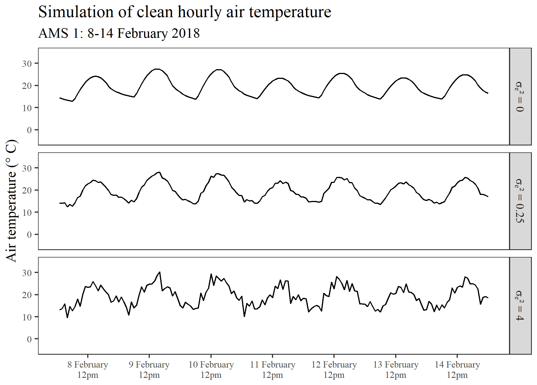
Figure 1An illustration showing a segment of the clean hourly air temperature series that was simulated for AMS 1, initially by deterministic modelling () and thereafter by incorporating stochastic error at each run using two differing set values for .
4.1.2 Introduction of aberrations
Observations were largely chosen at random for the purpose of concurrently introducing numerous varying aberrations into the clean simulated data (in order to replicate the type of error-prone series considered in this paper). Once selected, the same observations were perturbed during each iteration of the study. Table 1 presents the set of 12 varied forms of aberration that were introduced simultaneously during each run, along with the corresponding AMS and time periods that were selected for perturbation. Aberrations 1 to 4 represent differing forms of solitary outliers (spikes or dips) that affect either a single AMS or multiple AMSs concurrently. Aberrations 5 to 9 represent varied forms of temporary level shifts in the series mean, each with a differing duration. Aberration 9 was deliberately designed to extend across more than half the time period of the data, with the expectation that all of the varying double-standardization procedures would break down in trying to detect it (even those procedures that employ robust statistics). Aberrations 10 to 12 represent periods of irregularity in the diurnal pattern, each of differing length. In certain instances, the same AMS was assigned to more than one aberration (e.g. AMS 3) to permit the evaluation of the proposed method against three alternatives in the simultaneous detection of multiple varying forms of outliers within a series.
Table 1An overview of the set of aberrations simultaneously introduced during each iteration of the simulation study as well as the corresponding observations that were randomly selected for perturbation in each instance.
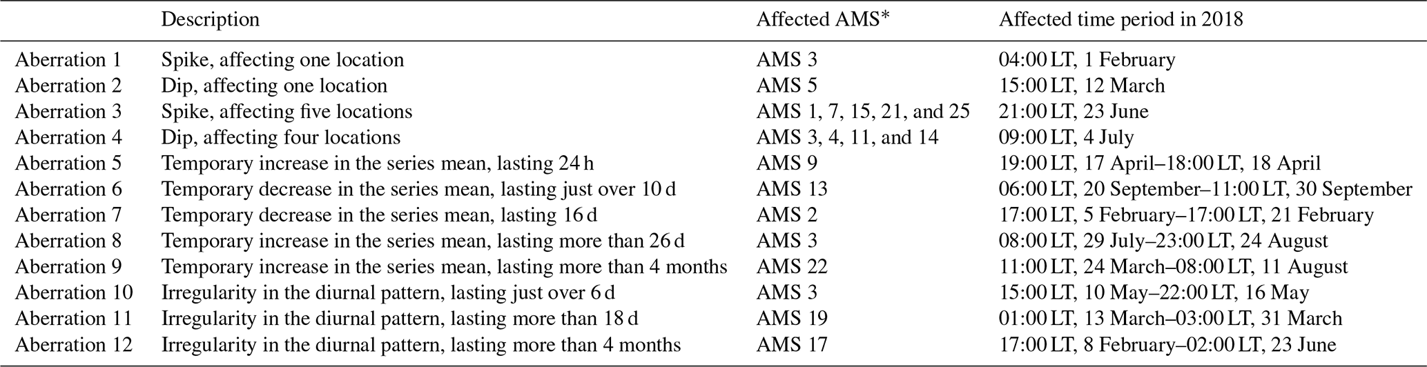
* Automatic monitoring station, i.e. spatial location.
Under each fixed value of (0.25 and 4), the set of aberrations shown in Table 1 was introduced at differing degrees of perturbation (mild, moderate, and severe). For spikes, dips, and level shifts in the series mean (i.e. aberrations 1 to 9), mild outliers were introduced by perturbing the relevant observations by ±5 °C, moderate outliers were introduced by perturbing the relevant observations by ±10 °C, and severe outliers were introduced by perturbing the relevant observations by ±15 °C. To achieve periods of irregularity in the diurnal pattern (i.e. aberrations 10 to 12), mild aberrations were introduced by shifting the respective periods of data backward by 4 h, moderate aberrations were introduced by shifting the respective periods of data backward by 8 h, and severe aberrations were introduced by shifting the period of data backward by 12 h (in which case a complete inversion of the diurnal pattern was achieved with air temperatures that were originally simulated for a timestamp of, say, 15:00 LT, reflecting a timestamp of 03:00 LT instead). To illustrate the manner in which irregular diurnal patterns were introduced into the clean data, Fig. 2 displays the simulation of aberration 10 under differing degrees of perturbation.
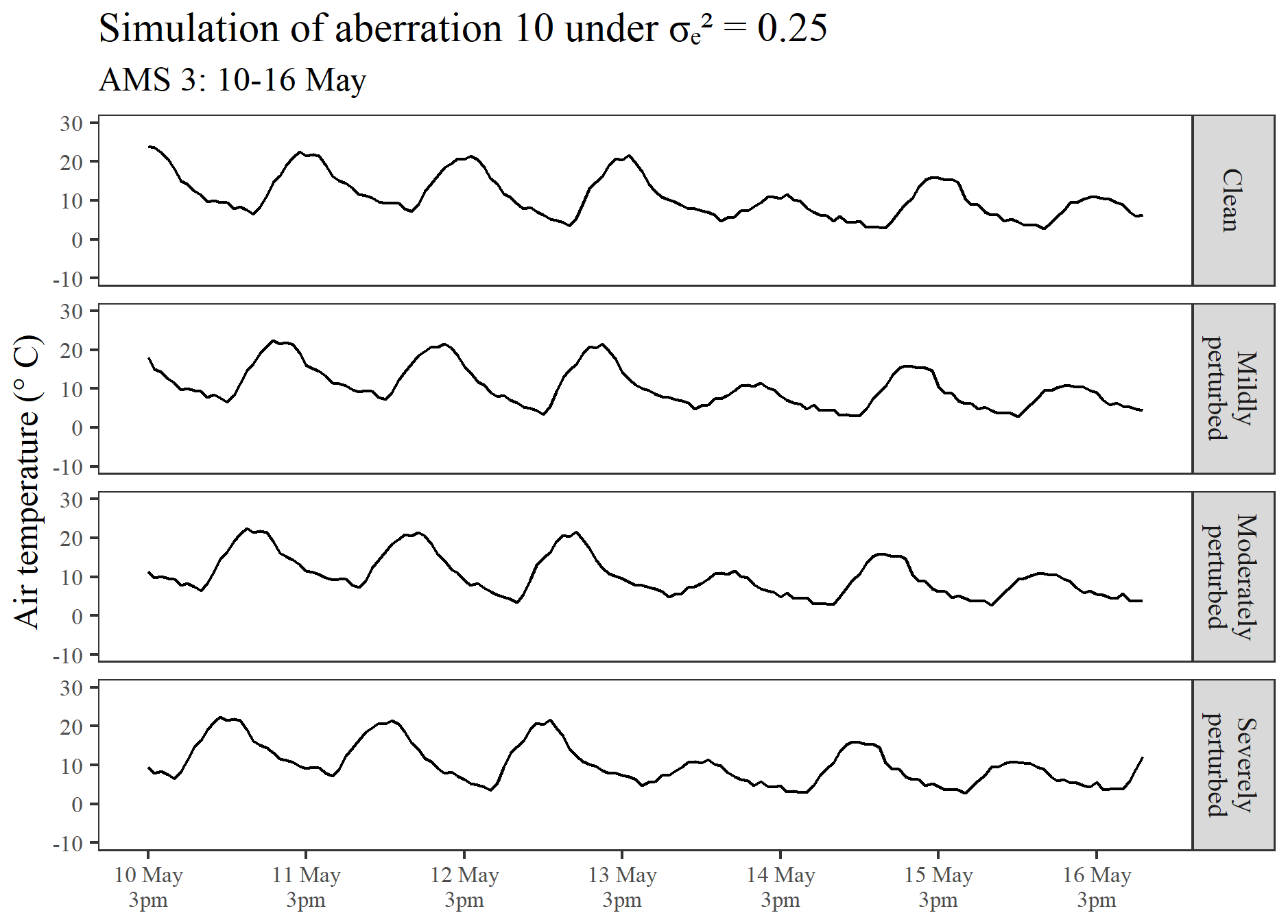
Figure 2An illustration showing the perturbation of a segment of the clean hourly air temperature series that was simulated for AMS 3, in the case, in order to introduce differing degrees of irregular diurnal patterns into the data.
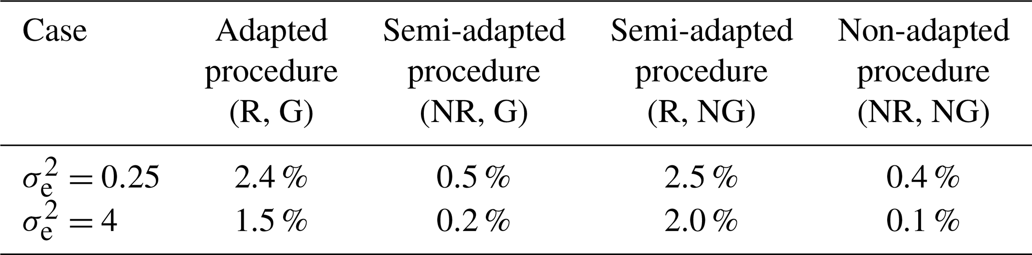
Thus, a total of six different scenarios were tested (two set values of degrees of perturbation). In each of the six scenarios, 100 aberrant data sets were simulated. The adapted double-standardization procedure was applied to each and every aberrant data set, and so too were the semi-adapted and non-adapted versions lacking either or both of the proposed procedural adaptations discussed in Sect. 3.1.
Hereafter, we use the abbreviation “R” to denote the use of robust statistics within a procedure, the abbreviation “NR” to denote the use of non-robust statistics, the abbreviation “G” to indicate the implementation of global series standardization, and the abbreviation “NG” to denote non-global or seasonally controlled series standardization.
4.2 Results of the simulation study
Before assessing the performance of each of the double-standardization procedures in the detection of the artificially imposed aberrations, we evaluated the clean data sets simulated under the two set values of (0.25 and 4). In particular, we explored the prevailing correlation between the clean series in each instance – both before and after preliminary series standardization using different methods – and we examined the rates of “false positives” (Zewotir and Galpin, 2007) that were obtained when the differing validation techniques were applied to the clean data. Finally, we also examined the autocorrelation functions (ACFs) and partial autocorrelation functions (PACFs) of the twice-standardized (clean) series in relation to that of the original series. The objective of this was to ascertain whether or not spatial standardization removes seasonal (diurnal) periodicity within a series, through implementation of either the adapted or non-adapted double-standardization procedure. A data set simulated for AMS 1, using a set value of , was arbitrarily chosen for this purpose.
4.2.1 Evaluation of the clean data sets
In the case, the temporal (Pearson) correlation prevailing between differing pairs of series within the spatial set was observed to range from 0.90 to 0.99 across all 100 iterations of clean data simulated for this scenario. In contrast, the prevailing temporal correlation between the series was observed to be somewhat lower in the case, ranging from 0.81 to 0.93 across all relevant iterations. The slightly weaker between-series correlation generated in this scenario is not surprising given the more erratic trend produced in each series in this case (as illustrated in Fig. 1). In light of the observed differences in correlation structure, we anticipated that there would be a lower rate of success in the detection of outliers in the case, given the formulation of the new procedure specifically for strongly correlated series. That is, the success rate of the new procedure was expected to be inversely proportional to the strength of the between-series correlation prevailing in the data.
Table 2Range of the observed temporal correlation between the one-time standardized series across all of the clean data sets simulated with each value of .
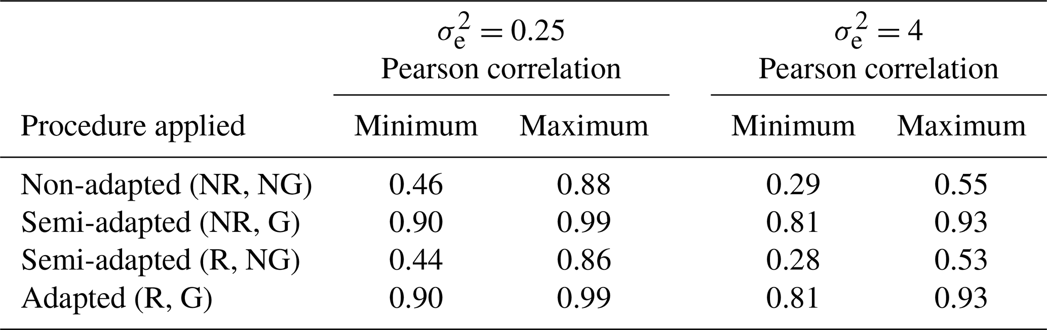
Table 2 displays the range of temporal correlations that continued to prevail between the clean series after preliminary standardization was implemented using differing methods (global versus seasonally controlled) but prior to spatial standardization. Under both set values of , it is evident from the table that the between-series correlation becomes depressed when a non-global (NG) or seasonally controlled approach is applied during preliminary series standardization. For example, in the case, it can be seen that the range of temporal correlation dropped from between 0.90 and 0.99 in the original data (as specified above) to between 0.46 and 0.88 when the non-adapted double-standardization procedure was applied to standardize each series independently (using a non-global approach and non-robust statistics). Similar results were achieved when a semi-adapted double-standardization procedure was applied using robust statistics, again using a non-global approach to independent series standardization. In contrast, it can be seen that the between-series correlation was preserved when a global approach was adopted to preliminarily standardize each series, regardless of whether or not robust statistics were used.
Once spatial standardization of the clean simulated data sets was subsequently implemented using the four differing techniques (i.e. after double standardization of the data was complete), we conducted an evaluation of the distribution of the resulting twice-standardized data in each case to determine the overall false-positive rate of outlier detection using each method. Furthermore, we examined the false-positive rates of detection, specifically among observations selected for eventual perturbation.
Similar to what we would expect to see in standard normal data, Table 3 shows that only a very low percentage of data (0.5 % or less, in each case on average) was flagged as outliers in each of the clean simulated sets when using double-standardization procedures that employ non-robust statistics along with a typical deviation threshold of h=3. However, methods that employ robust statistics during preliminary and spatial standardization were found to yield somewhat higher overall false-positive rates of detection in each case when applied to the clean simulated data. This highlights a slight weakness of the new outlier detection procedure proposed for strongly correlated data, which is indicative of lower levels of efficiency. Moreover, this finding infers that a slightly higher deviation threshold might need to be applied when using this procedure (or any other procedure that employs robust statistics to standardize data) in order to avoid having to inspect (unnecessarily) a very large number of flagged observations. Nonetheless, we chose to proceed with the simulation study, largely using a deviation threshold of h=3, but we also opted to explore detection rates based on a higher deviation threshold of h=5 for the adapted procedure only. Fortunately, despite the apparent tendency of robust outlier detection methods to yield a higher number of false positives, the results presented in Appendix B (see Tables B1 and B2) confirm that virtually no bias was introduced at the start of the study, with false-positive rates being zero or negligible among observations specifically chosen for eventual perturbation.
Table 3Percentages of clean data lying >3 standard deviations from the mean after double standardization of the data using differing procedures (averaged across all 100 simulated data sets relating to each case).
The ACF plots displayed in Figs. 3–5 were used to determine whether or not the seasonality present within a series (see Fig. 3) is ultimately removed via spatial standardization of the data across series at each point in time, using either the adapted (R, G) or non-adapted (NR, NG) double-standardization procedures (see Figs. 4 and 5 respectively). The plots are arbitrarily based on a clean hourly air temperature series that was simulated for AMS 1 in the case (previously shown in Fig. 1). The differing ACF plots of the resulting twice-standardized data, shown in Figs. 4 and 5 respectively, indicate that the spatial standardization of the data serves to greatly reduce the seasonal trend, regardless of whether it is performed using the adapted technique or the non-adapted technique. (The corresponding PACF plots given in Appendix C lead to similar conclusions.) However, it is equally clear from the ACF plots that spatial standardization does not remove seasonality entirely. Furthermore, the ACF associated with the twice-standardized data arising from the adapted procedure (R, G) is seen to decay extremely slowly, indicating strong dependencies between the twice-standardized data values through to very long hourly lags. One would thus expect the adapted procedure to perform well in the detection of extended sequences of consecutive outliers. In contrast, it can be seen that the ACF associated with the twice-standardized data arising from the non-adapted procedure (NR, NG) decays far more rapidly, indicating a greater degree of stationarity, likely due to preliminary series standardization having been performed in a seasonally controlled manner too.
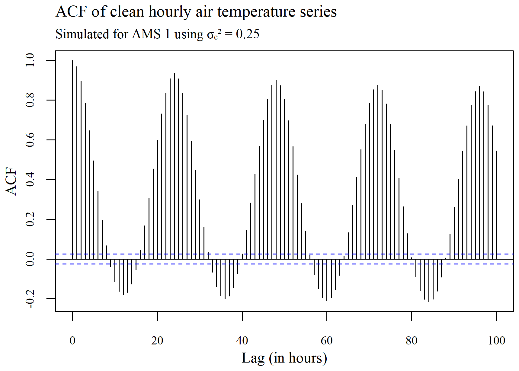
Figure 3Plot of the autocorrelation within a series of clean hourly air temperature data simulated for AMS 1, using .
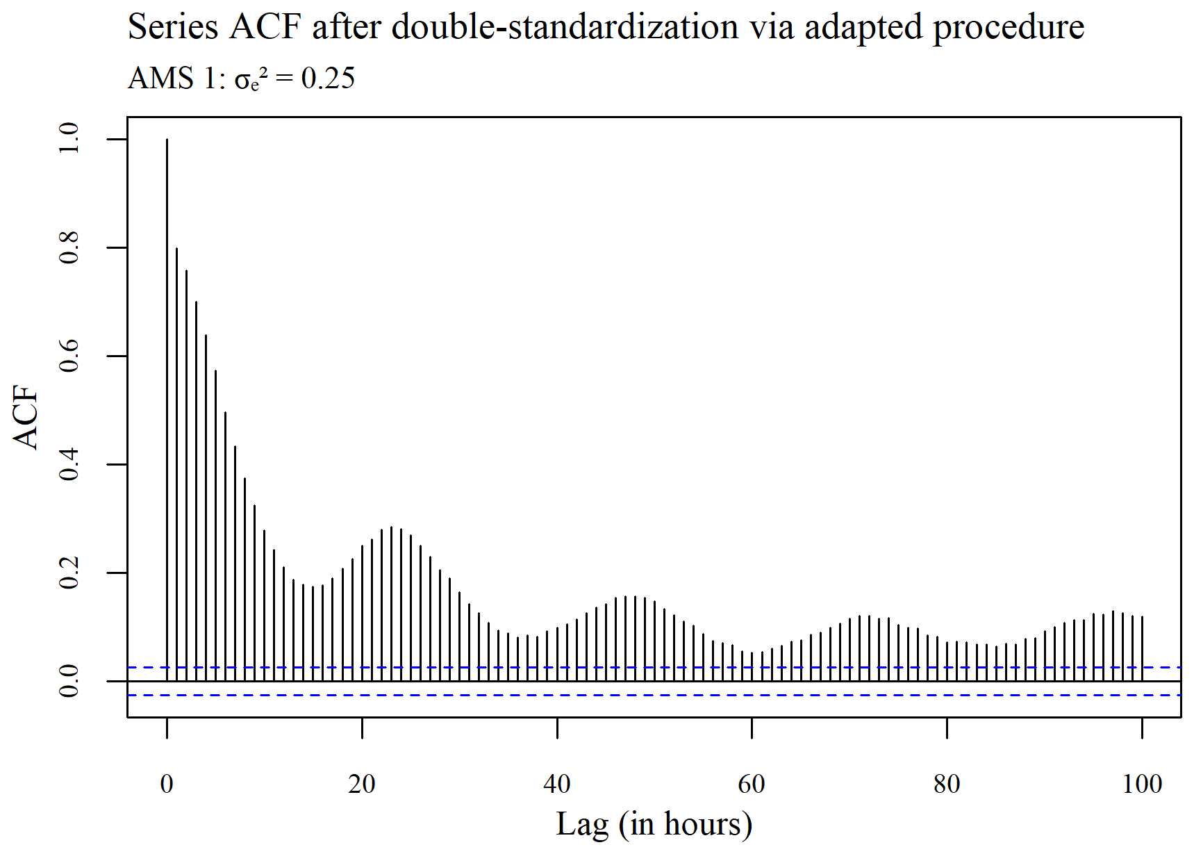
Figure 4Plot of the autocorrelation in the series, after double standardization of the data using the adapted procedure.
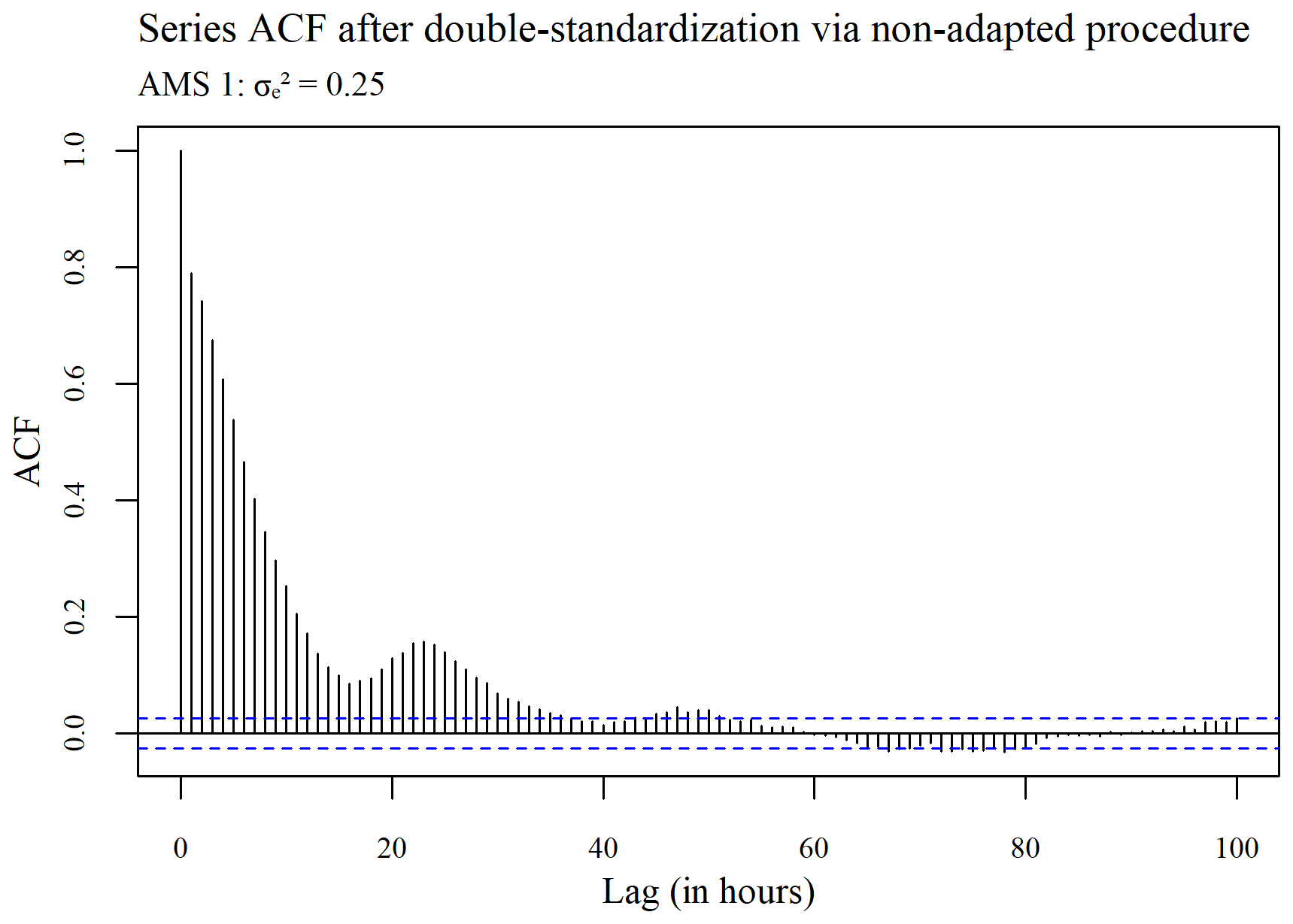
Figure 5Plot of the autocorrelation in the series, after double standardization of the data using the non-adapted procedure.
4.2.2 Results when aberrations were introduced
Tables 4–7 display the success rates of the four validation procedures in detecting the various aberrations that were simultaneously introduced into the clean data under six different scenarios (two set values of degrees of perturbation). For single outliers (i.e. aberrations 1 and 2), the success rate shown refers to the proportion of iterations in which the respective aberration was detected (from a relevant set of 100 runs). For solitary outliers affecting multiple locations (i.e. aberrations 3 and 4), the success rate reflects the proportion of aberrant observations that were detected each time on average. For sequential outliers (i.e. aberrations 5 to 12), the success rate reflects the proportion of the perturbed sequence that was detected each time on average.
Table 4Results showing the success rates of the non-adapted double-standardization procedure (NR, NG) in detecting each aberration among the 100 iterations in each scenario.
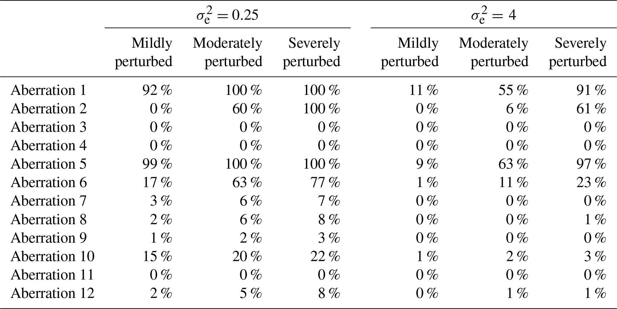
Table 5Results showing the success rates of the semi-adapted double-standardization procedure (NR, G) in detecting each aberration among the 100 iterations in each scenario.
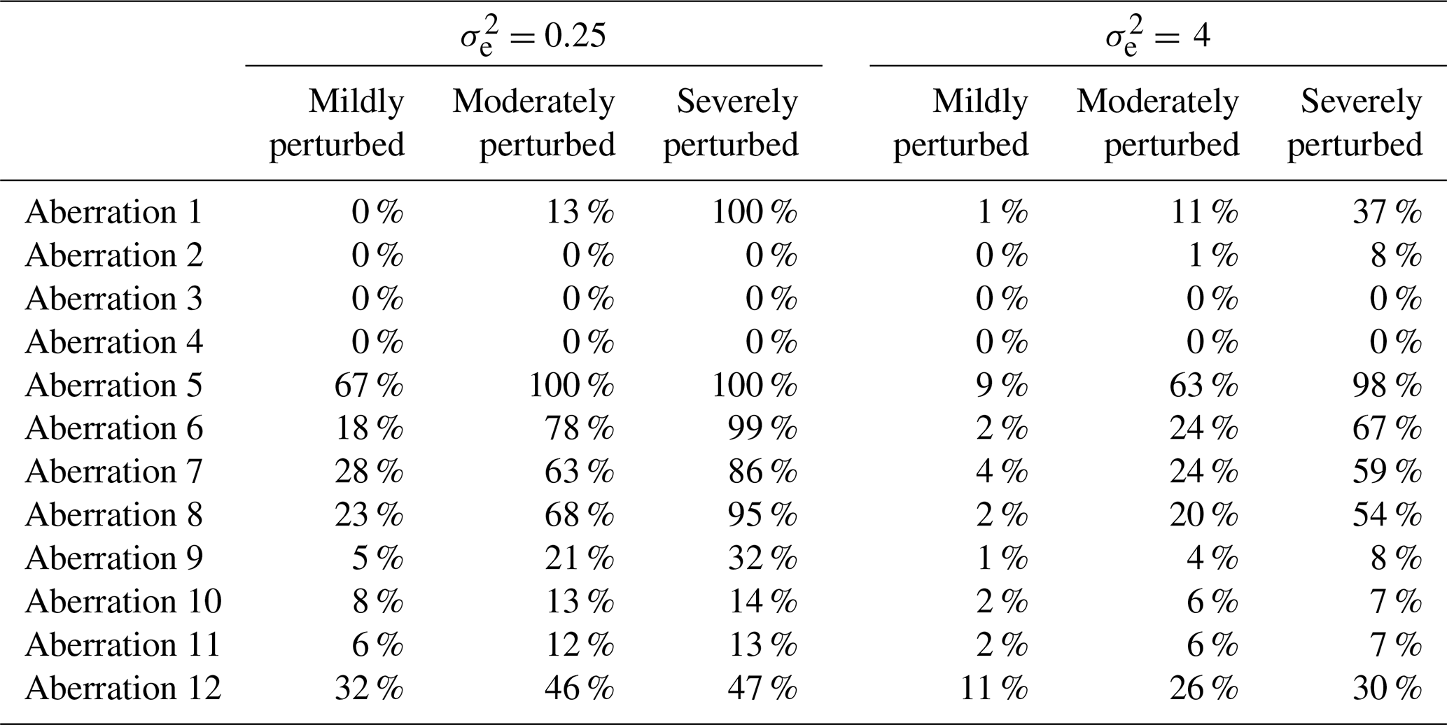
Table 6Results showing the success rates of the semi-adapted double-standardization procedure (R, NG) in detecting each aberration among the 100 iterations in each scenario.
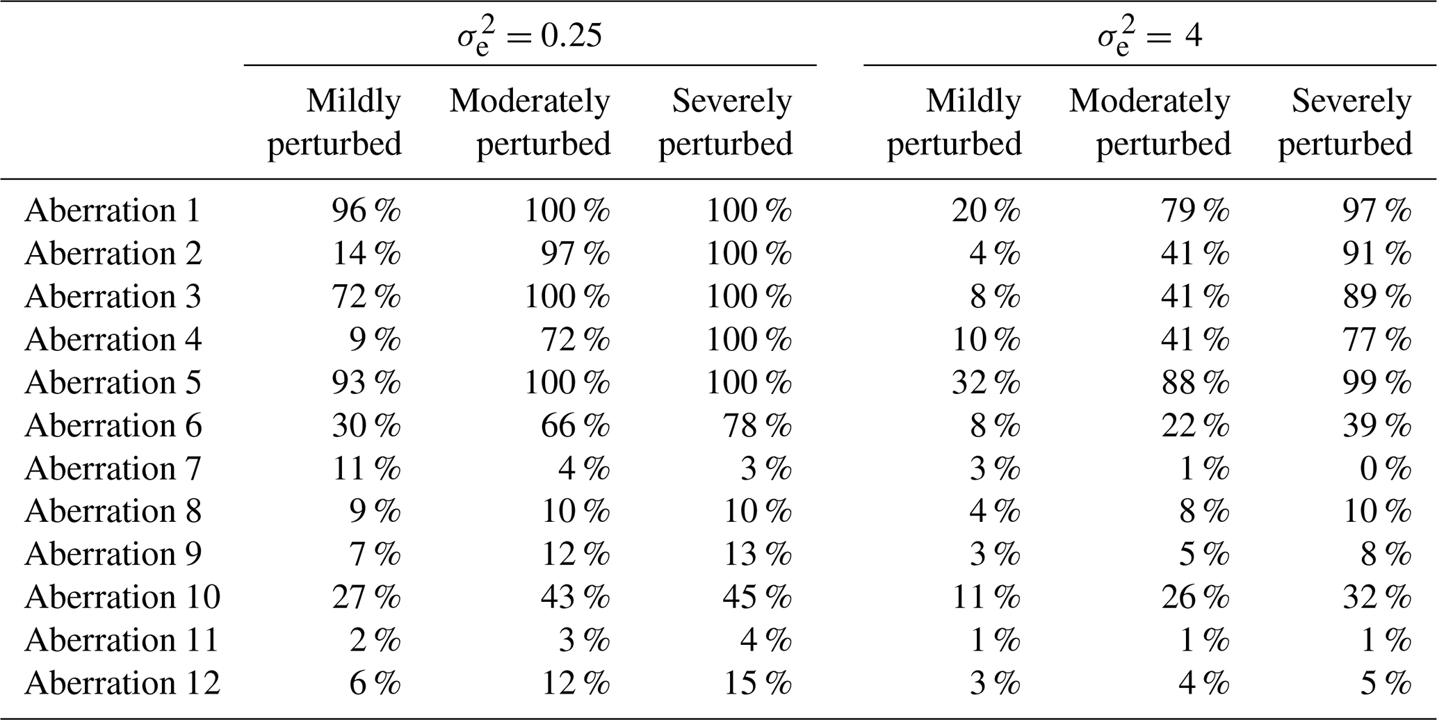
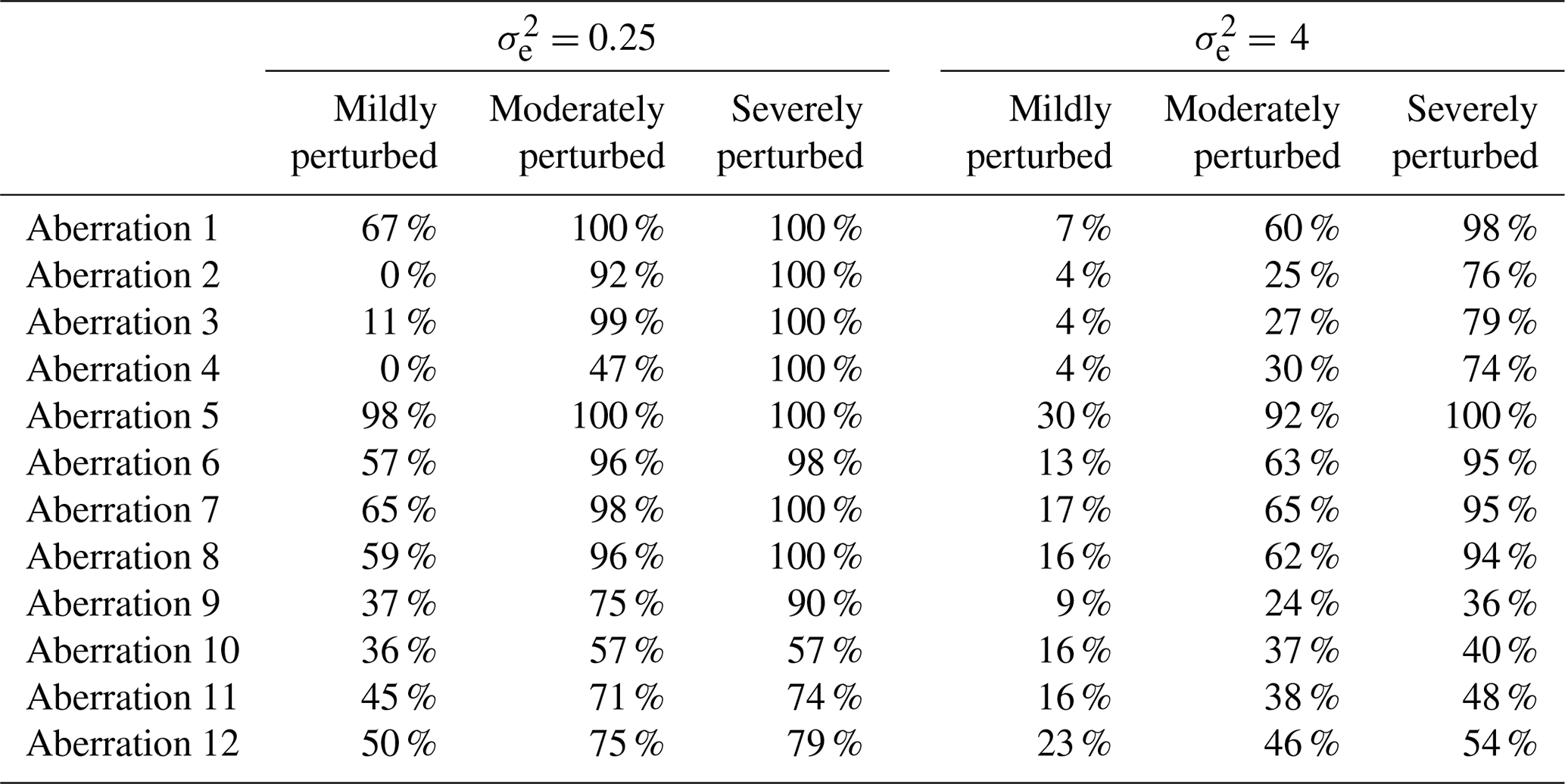
Table 7Results showing the success rates of the adapted double-standardization procedure (R, G) in detecting each aberration among the 100 iterations in each scenario.
The results presented in Table 4, in the case, show that the non-adapted double-standardization procedure (NR, NG) was highly reliable in the detection of aberration 1 (a solitary spike affecting only one location) and aberration 5 (a temporary increase in the series mean of very short duration). Under conditions of moderate to severe perturbation, the method also performed well in the detection of aberration 2 (a solitary dip affecting a single location) and aberration 6 (a temporary decrease in the series mean lasting slightly longer than aberration 5 but still only persisting for less than half a month). However, the non-adapted method performed poorly in the detection of irregular patterns (i.e. aberrations 10 to 12) and also failed to detect any substantial portion of any sequence of level shift lasting more than several days (i.e. aberrations 7 to 9). Furthermore, the non-adapted double-standardization procedure was completely unsuccessful in detecting aberrations 3 and 4, consisting of solitary outliers affecting multiple locations concurrently.
We largely attribute the generally poor performance of the non-adapted method in the detection of sequential outliers to the seasonally controlled approach that this technique uses to implement preliminary series standardization. As we showed in Sect. 4.2.1, this depresses the temporal correlation within the data by reducing the dependencies between consecutive values in each standardized series, in order to render them somewhat stationary. Furthermore, performing preliminary series standardization within smaller seasonally controlled subsets of data, using non-robust estimates, raises the risk of introducing bias when consecutive outliers are present within the series for extended periods. Similarly, we attribute the poor performance of the non-adapted method in the detection of aberrations 3 and 4 to the use of non-robust estimates for the spatial mean and standard deviation of the data at each time point and hence to the introduction of bias into the twice-standardized data during spatial standardization. When the spatial sample is small (e.g. only 25 locations), outliers that affect multiple locations concurrently will substantially bias the spatial mean and standard deviation of the data for the time point in question.
Overall, it is fair to state that the non-adapted double-standardization procedure was not at all comprehensive in detecting the varied set of aberrations that were simultaneously introduced into the data in the case. Furthermore, when weaker temporal correlation prevailed between the simulated series in the case, the procedure was even less sensitive to the presence of all forms of aberration that were introduced.
Tables 5 and 6 display the corresponding rates of success for semi-adapted versions of the double-standardization procedure. The results presented in Table 5 confirm that the implementation of a global approach to preliminarily standardize each series drastically improves the ability of a double-standardization procedure to detect a substantial portion of any sequence of level shift – even those with very long durations – and particularly under conditions of moderate to severe perturbation (see aberrations 5 to 9 in Table 5). However, with the continued use of non-robust statistics, a semi-adapted double-standardization procedure (NR, G) still struggles in general with the detection of irregular patterns (i.e. aberrations 10 to 12), though there was a notable increase in the average proportion of the sequence being detected in relation to aberration 12. Furthermore, such a semi-adapted procedure (NR, G) was found to be largely incapable of detecting solitary outliers (i.e. spikes and dips), with the exception of aberration 1 under conditions of severe perturbation in the case.
In contrast, the results presented in Table 6 highlight that a semi-adapted procedure (R, NG) which adopts the use of robust statistics for data standardization is highly reliable in the detection of all forms of solitary outliers under conditions of moderate to severe perturbation, in the case. This is true even for spikes and dips that affect multiple locations concurrently, i.e. aberrations 3 and 4. However, with the continued implementation of seasonally controlled series standardization, such a semi-adapted procedure (R, NG) remains unreliable in the detection of irregular patterns (i.e. aberrations 10 to 12) and in the detection of substantial portions of any sequence of level shift that has an extended duration (i.e. aberrations 7 to 9).
Table 7 displays the corresponding performance of the (fully) adapted double-standardization procedure (R, G). In the case, the adapted method was found to be highly reliable in detecting all forms of solitary outliers and level shifts (i.e. aberrations 1 to 9) under moderate to severe perturbation, and it was seen to display reasonable performance in detecting such perturbations when mild. (One slight exception was in the detection of aberration 4 under conditions of less than severe perturbation.) The adapted method performed unexpectedly well in detecting the vast majority of the lengthy sequence associated with aberration 9. It had been anticipated that all four double-standardization procedures – even those employing the median and MAD – would break down in the detection of aberration 9, given that this level shift extends for more than half the time period of the data.
Moreover, unlike the other methods, the adapted double-standardization procedure was able to detect large portions of the irregular diurnal patterns that were introduced via aberrations 10 to 12, particularly when the shift in the diurnal pattern was of a moderate to severe degree (i.e. 8 to 12 h). Detection rates of 100 % are not really achievable in the case of irregular diurnal patterns when using a form of double-standardization procedure for data validation. This is true even under severe perturbation (or complete diurnal inversion), when maximum temperatures are logged as having occurred in the early hours of the morning and minimum temperatures during the afternoon. This is due to the fact that readings time-stamped closer to either sunrise or sunset generally will not be flagged, as a result of their values being similarly moderate and comparable (e.g. an air temperature measured at 18:00 LT mistakenly logged with a timestamp of 06:00 LT would probably not appear extreme for a timestamp of 06:00 LT or deviate too far from that recorded elsewhere at 06:00 LT). However, provided a sufficient portion of the irregular diurnal pattern is flagged by the double-standardization procedure, it is usually quite easy to detect the corresponding start and end points.
Overall, the adapted procedure (R, G) displayed either equivalent or superior performance compared to the alternative methods in detecting all forms of severe perturbation and almost all forms of moderate perturbation (with a slight exception in the case of aberrations 2 and 4, where the semi-adapted procedure (R, NG) achieved slightly higher rates of detection, though all four procedures struggled somewhat, specifically in the detection of aberration 4 under conditions of less than severe perturbation, possibly due to a mere peculiarity of the observations selected for this aberration). The adapted method also displayed superior performance in the detection of mildly perturbed sequences, including both level shifts and irregularities in the diurnal pattern. However, it was outperformed by the semi-adapted procedure (R, NG) in the detection of mild spikes and dips (i.e. aberrations 1 to 4) and by the non-adapted procedure in the detection of aberration 1 under mild perturbation only. Thus, it would seem that procedures which implement a seasonally controlled approach to preliminary series standardization possess superior sensitivity in the detection of solitary outliers that are milder. However, this is hardly an advantage when they are unable to detect even the most severe forms of sequential outliers of any substantial duration.
In the case, the adapted double-standardization procedure was still found to be highly reliable in the detection of severe perturbations in almost all of the instances, with fair performance being displayed in the detection of moderate perturbations. In the case, when a higher deviation threshold of h=5 was applied, the adapted procedure only failed to detect 20 % of the severe perturbations that it had successfully identified using a deviation threshold of h=3, although an additional 38 % of moderate perturbations went undetected (see Table D1).
As presented in the case study that follows, we next applied the adapted double-standardization procedure to the set of hourly air temperature series actually recorded by AMS 1 to AMS 28 between 1 February and 30 September 2018. The hourly data were extracted from SAAQIS, and although the degree of error present within each time series was unknown, it was considered to be potentially substantial and have varying forms. For context, SAAQIS serves as a publicly available online platform for storing and reporting on data for a wide range of air pollutant and meteorological variables that are measured via a country-wide network of AMSs under the ownership of differing public entities. Such stations depend on the use of programmable data-recording devices that concurrently measure a variety of sensors for differing variables at highly frequent and regular intervals over extended periods and that are additionally configured to process and transmit the data (Campbell Scientific, 2024). The choice of sensors, rates of raw measurement (e.g. every few minutes or seconds), and time spans for subsequent calculation of recorded values (e.g. hourly readings) is customizable for each station. The resulting time series made available on SAAQIS are hence analogous to the type of data described in Sect. 1 as being susceptible to multiple forms of error.
5.1 Overview of the data
In the case study, we chose to retain AMS 6, AMS 23, and AMS 24 within the spatial time series set despite a high degree of missingness in their respective series. We thus obtained, to varying degrees of completeness, a total of 28 series of average air temperature readings processed for every hour of every day by the respective AMSs positioned at different locations across the Gert Sibande and Nkangala districts of the province of Mpumalanga (see Fig. 6). Six AMSs among the 28 were identified as being of the utmost relevance (hereafter referred to as principal stations), i.e. AMS 9, AMS 10, AMS 12, AMS 15, AMS 21, and AMS 26. These stations were deemed to be of principal importance based on their respective proximities to six different primary schools from which repeated-measure health data had been collected during 2018. The remaining 22 AMSs were regarded as less pertinent (hereafter referred to as subsidiary stations).
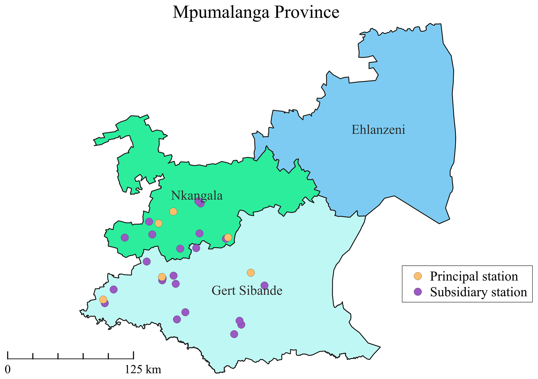
Figure 6Map showing the locations of the 28 AMSs used to record ambient air temperature in MP in South Africa during 2018.
The temporal correlation prevailing between differing pairs of series within the spatial set was determined to range between 0.88 and 0.99, with only the subsidiary series recorded at AMS 24 exhibiting deviant behaviour. In particular, this series was found to display a temporal correlation of less than 0.20 with all other series in the spatial set, raising doubts about the validity of the data within that series. Such a finding highlights the reality, in general, that any series external to the primary interests of a study will also be susceptible to error and should consequently not be used in isolation as a reliable reference for validating the series of principal importance. This notwithstanding, low correlation coefficients must always be interpreted with caution prior to data pre-processing, since temporal correlation between series can be drastically impacted merely by the presence of a few extreme data points (Walker, 1960). Thus, it was decided that, regardless, AMS 24 should be retained within the spatial set.
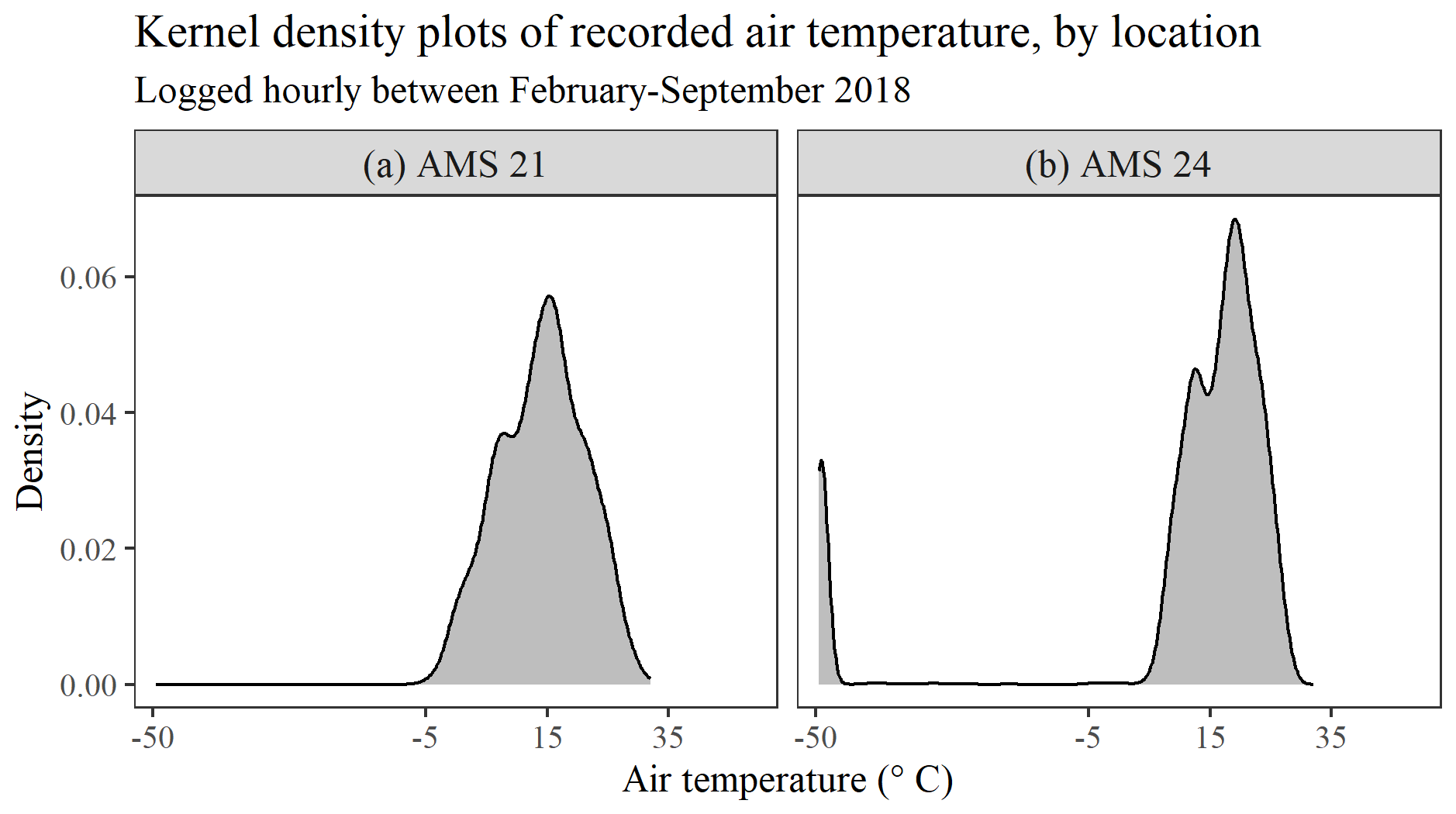
Figure 7(a, b) Estimated probability density function of air temperature at two different locations in the province of Mpumalanga, based on average hourly data logged by AMS 21 (a) and AMS 24 (b) between February and September 2018.
Despite the evidence of a predominantly strong temporal correlation between series, considerable variation was observed in the level of air temperature recorded by the 28 AMSs at discrete points in time. For instance, the air temperatures logged across the 28 different locations between 16:00 and 17:00 LT on 2 February 2018 displayed an interquartile range of 8.3 °C and ranged from as high as 31.7 °C at AMS 26 to as low as 17.4 °C at AMS 11 only 64.0 km away. Such an observation emphasizes the necessity, in general, of preliminarily standardizing each series independently according to its own distribution. However, despite the observed differences, each of the series was confirmed as exhibiting an approximately symmetric distribution of much the same shape, akin to that displayed in Fig. 7a for the series recorded at AMS 21. Even the series recorded at AMS 24 was found to display a distribution of a similar form, as seen in Fig. 7b, aside from the presence of a deviant cluster of extreme outliers situated on the far left, which was subsequently determined to be the result of multiple periods of prolonged instrument malfunction (shown later in Sect. 5.3). Thus, for the purpose of detecting any and all forms of outliers present within the wider spatio-temporal data set, it was deemed viable to apply the proposed double-standardization procedure (R, G) precisely as defined in Eqs. (2) and (3), i.e. by implementing a MAD approach during both stages of data standardization.
Unlike in the simulation study, the double standardization of the data in the case study was performed using Microsoft Excel 2016, given that it facilitates the flagging of outliers more easily via conditional formatting. To once again permit a comparative evaluation of the findings, the non-adapted and semi-adapted double-standardization procedures were also applied to the same univariate spatial set of hourly air temperature series. In each case, no prior data cleaning of any sort was performed. The overall effectiveness in the detection of outliers was assessed in terms of three aspects, i.e. sensitivity (measured by the extent of data flagged as potentially inaccurate), efficiency (determined by the percentage of flagged values confirmed to be inaccurate), and the level of comprehensiveness (based on the absolute number of inaccurate observations and the variety of aberrations detected). Comparative figures were generated in R using the ggplot2 package developed by Wickham (2016).
5.2 Summary of the findings
After double standardization of the data was performed using the adapted procedure (R, G), a total of 3135 twice-standardized air temperature values (2.2 % of all non-missing data) were noted to exceed a deviation threshold of h=3 such that . Of these, 1399 values (1.0 % of all non-missing data) were found to exceed a deviation threshold of h=4. Given the likelihood of a high number of false positives (based on the results of the simulation study), we chose to restrict our investigation to the 1399 more extreme values – the majority of which were observed to appear in consecutive sub-sequences within a select few of the (principal and subsidiary) air temperature series, including AMS 24.
Despite the primary aim being the validation of each principal series, an inspection was conducted of every one of the flagged points and sequences in order to more thoroughly assess the efficiency and comprehensiveness of the adapted procedure in detecting varying types of outliers. Of the 1399 air temperature values that were flagged, a total of 763 (54.5 %) were deemed to reflect data error after in-depth interrogation (a detailed discussion of certain findings is provided in Sect. 5.3). An additional 103 data values were further deemed invalid after noting that they formed part of differing extended sub-sequences – only portions of which had been flagged by the procedure. Ultimately, a total of 886 air temperature values were nullified, with only 24 of these being solitary outliers recorded by varying AMSs (both principal and subsidiary) at differing time points. Another 294 of the nullified values were comprised of a sub-sequence displaying an apparent inversion in the diurnal pattern which occurred at AMS 15 (a principal station). The remainder (566 nullified values) were comprised of 11 different sub-sequences representing periods of abnormal level shifts in four different series (both principal and subsidiary), ranging from as short as 2 h to as long as 304 h. The findings from the simulation study in Sect. 4 provide assurance that any other data errors not detected by the adapted procedure in this case study would likely only be solitary spikes and dips of milder perturbation and hence of lesser consequence.
The comparative analysis in Table 8 highlights that the non-adapted and semi-adapted versions of the double-standardization procedure were considerably less comprehensive in detecting the same assortment of errors using a consistent deviation threshold of h=4. The non-adapted procedure (NR, NG) was determined to be the least sensitive and comprehensive. The semi-adapted procedure (R, NG) was found to be the most sensitive but least efficient, with the highest number of false positives. In line with the findings of the simulation study, this procedure was specifically observed to be less reliable in the detection of sequential outliers, flagging less than half of what the adapted procedure (R, G) had successfully been able to detect. However, the majority of the solitary spikes that were flagged by the adapted procedure were also detected by this procedure (17 out of 24). Conversely, the semi-adapted procedure (NR, G) was found to be somewhat more efficient, though less comprehensive, than the (fully) adapted procedure. As per the observations from the simulation study, this procedure was particularly weak in detecting solitary spikes (only 4 out of the 24 identified) and also somewhat less reliable in the detection of sequential outliers (73 % identified of those flagged by the fully adapted procedure).
Table 8Comparative analysis of the effectiveness of differing double-standardization procedures in detecting multiple varying forms of outliers.
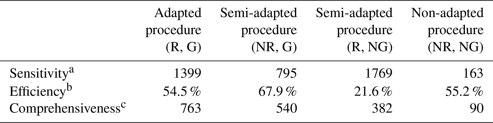
a Number of data points flagged as potential errors; that is, . b Percentage of flagged data points confirmed to be errors. c Total number of invalid data points detected.
It might be argued that the results for the non-robust double-standardization procedures in this case study would have been better if a more typical threshold of h=3 had instead been applied for these techniques in particular. However, the comparative figures shown below in Sect. 5.3 highlight that, even with the use of such a lower deviation threshold, the non-robust procedures would still have missed many aberrant observations that the adapted procedure was successfully able to detect using a deviation threshold of h=4. The findings of the simulation study further support this.
5.3 Examples of specific findings
Figure 8d highlights the superiority of the adapted procedure in identifying moderate air temperature spikes of between 9 and 10.5 °C that occurred concurrently at AMS 15, AMS 21, and AMS 23 between 09:00 and 10:00 LT on 2 February 2018. For example, the twice-standardized value of 6.0 obtained for AMS 21 corresponds to a supposed average air temperature of 28.3 °C between 09:00 and 10:00 LT. This reading was 9.3 °C higher than the average air temperature recorded during the hour prior, between 08:00 and 09:00 LT, and 3.5 °C higher than the average air temperature recorded during the subsequent hour, between 10:00 and 11:00 LT. The nearest neighbouring station to AMS 21 (AMS 17) did not record any such spike, despite being only 2.7 km away. The spikes at AMS 15, AMS 21, and AMS 23 were subsequently deemed invalid after noting that unfeasible readings were simultaneously being reported for other variables at these three stations, e.g. relative humidity in excess of 130 %. However, the corresponding twice-standardized air temperature values shown in Fig. 8a and b that were derived using non-robust double-standardization procedures failed to surpass even a lower deviation threshold of h=3. With the affected AMSs being under the same ownership, it is probably not coincidental that they suffered from similar errors across multiple sensors over the same period of time despite being situated more than 100 km apart. Several such spikes were detected at differing time points within the data set and for differing AMS groups.
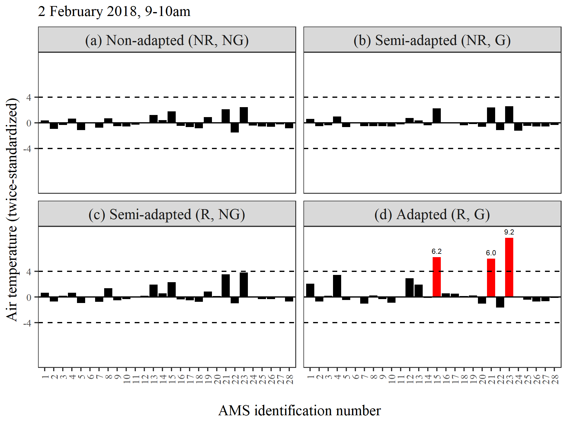
Figure 8(a–d) A comparison of the twice-standardized air temperature values obtained for each AMS between 09:00 and 10:00 LT on 2 February 2018, derived using four differing double-standardization procedures employing either robust (c, d) or non-robust (a, b) statistics and either a seasonally controlled (a, c) or global (b, d) approach to series standardization.
Figure 9a–d highlight the detection of a temporary level shift down in air temperature at AMS 1. Subsequent inspection of the relevant portion of non-standardized data revealed that air temperature at this location supposedly dropped by more than 6 °C to 13.9 °C at midday on 6 April 2018 and then plummeted further to just below freezing (−0.9 °C) at 13:00 LT. Air temperature readings increased slightly thereafter but still remained 5–20° lower versus those recorded at all other AMSs for the next 22 h, before returning to normative levels at 13:00 LT on 7 April 2018. Each of the double-standardization procedures displayed some success in identifying this sequence, most likely due to its very short duration (based on the findings from the simulation study).
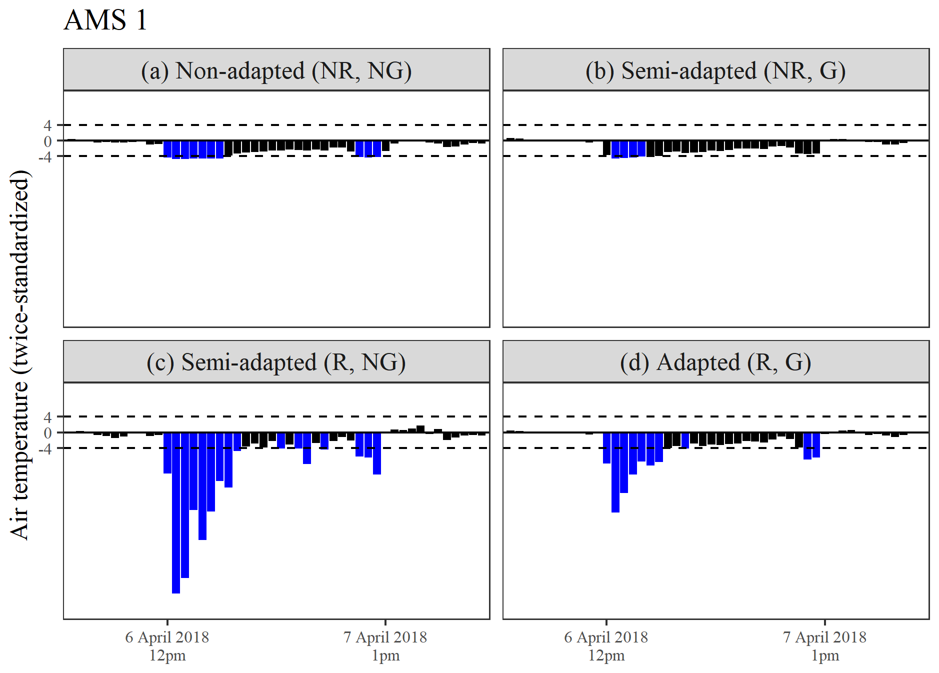
Figure 9(a–d) A comparison of the twice-standardized air temperature series obtained for AMS 1 between 6 and 7 April 2018, derived using four differing double-standardization procedures.
Figure 10d emphasizes the robustness and sensitivity of the adapted procedure in detecting prolonged periods of device malfunction at AMS 24. Air temperatures below −48 °C were reported at this location between 01:00 LT on 10 April and 08:00 LT on 12 April and again between 18:00 LT on 13 April and 08:00 LT on 26 April during 2018 (reflected by twice-standardized values as low as −171 beyond the axis limits of Fig. 10). Similar errors also occurred during September (not depicted). This finding explains the previously observed deviation of AMS 24 from the between-series temporal correlation structure. Procedures adopting a seasonally controlled approach to series standardization broke down in this scenario, as seen in Fig. 8a and c, even when robust MAD estimates were used. This is due to the fact that the malfunction persisted for more than 15 d in total during April (at least between 01:00 and 08:00 LT), resulting in fewer valid air temperature values being flagged as excessively large.
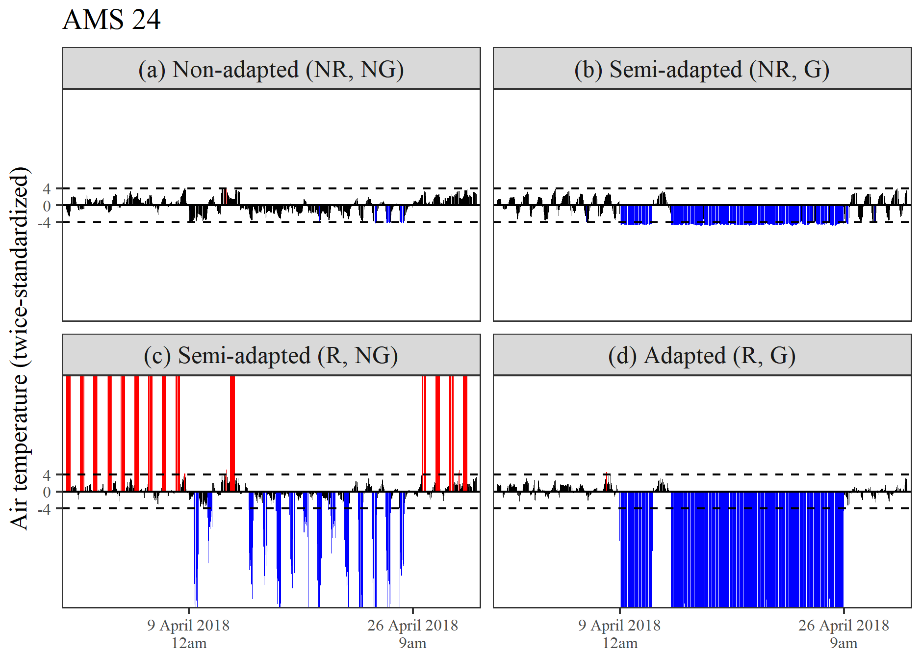
Figure 10(a–d) A comparison of the twice-standardized air temperature series obtained for AMS 24 during April 2018, derived using four differing double-standardization procedures.
Figure 11d highlights the superiority of the adapted procedure in detecting an inversion in the diurnal pattern at AMS 15 (a principal station), which occurred between 07:00 LT on 13 February and noon on 25 February 2018. During this period, maximum temperatures were logged as occurring at night and minimum temperatures during the day. The adapted procedure flagged 63 % of this sub-sequence. As expected, readings time-stamped closer to either sunrise or sunset were generally not flagged due to their more moderate and comparable values. Figure 11a and b show that procedures using non-robust estimates were naturally less sensitive to the period of timestamp error. Figure 11c further shows that detection was also inhibited by seasonally controlled series standardization, with the semi-adapted procedure (R, NG) only flagging 23.5 % of this sequence.
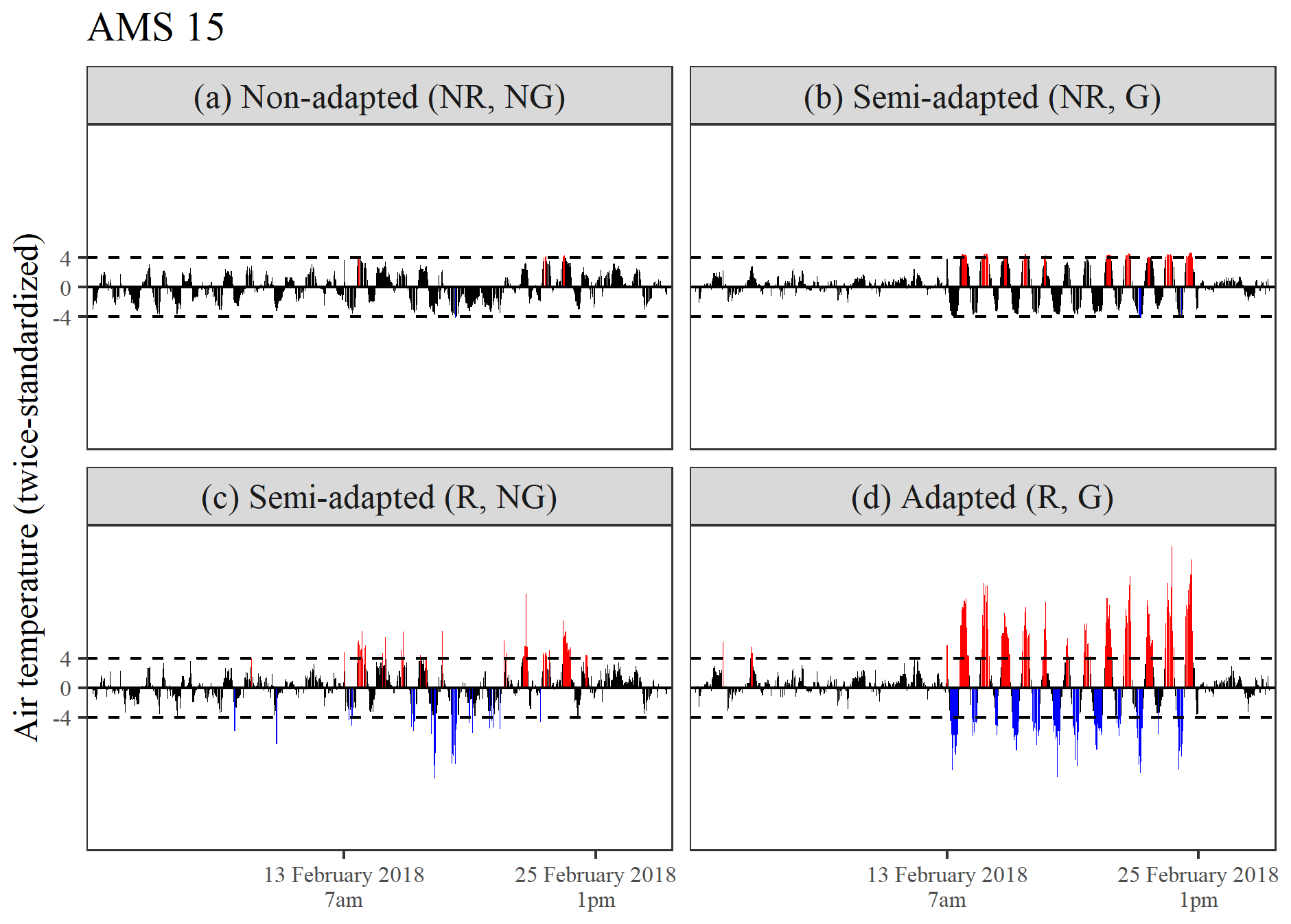
Figure 11(a–d) A comparison of the twice-standardized air temperature series obtained for AMS 15 during February 2018, derived using four differing double-standardization procedures.
In this paper, we have presented a new method for standardizing meteorological sensor data, with the purpose of enabling comprehensive detection of multiple varying forms of outliers in strongly correlated series that typically come from high-frequency measurements collected across different locations over an extended period of time. A review of the relevant literature characterized existing outlier detection techniques as sub-optimal for the validation of such error-prone spatial time series, as they each tend to cater to the detection of only one form of outlier in isolation, lack robustness, or fail to optimally leverage the strong between-series correlation that often prevails in high-frequency meteorological data exhibiting multiple seasonalities.
To address this problem, we have thus devised a nimble technique for the detection of both solitary and sequential outliers (including irregular patterns) in strongly correlated univariate spatial time series. In particular, we have made adaptations to an existing double-standardization procedure for more moderately correlated series that relies on a z-score approach. The modified procedure that we have proposed draws on robust statistics to estimate the mean and standard deviation of each respective temporal and (thereafter) spatial series to ensure sensitivity of detection even when extensive error is present within the data. Provided that each time series has a similarly shaped symmetric distribution, we advocate for the use of the most robust MAD approach to estimating the true mean and standard deviation of the data. Whilst the application of such robust statistics in the detection of outliers is nothing new, to the best of our knowledge the adoption of the MAD method in a double-standardization procedure is unusual. Furthermore, the proposed procedure is somewhat unique in that the MAD technique is applied to highly seasonal, non-stationary time series using a global approach that retains the series structure rather than controlling for seasonality or implementing Hampel's rolling window. Accordingly, the new method preserves and fully leverages the temporal correlation between series by retaining dependencies between consecutive values in the twice-standardized data. This facilitates better detection of more lengthy aberrant sequences, including the detection of seemingly typical data points occurring outside the diurnal cycle.
Both procedural adaptations mentioned above have been shown to be necessary for achieving optimal rates of detection when varying forms of aberration are potentially present within a data set, including irregular patterns. When tested on simulated data marred by artificially imposed aberrations, double-standardization procedures which adopted a global approach to preliminary series standardization generally outperformed those that implemented seasonally controlled series standardization in the detection of sequential outliers lasting more than just a few days. Conversely, procedures which employed robust statistics to standardize the data generally outperformed procedures that did not in the detection of solitary outliers and level shifts with very short durations. Overall, the (fully) adapted double-standardization procedure (R, G) displayed either equivalent or superior performance compared to the non-adapted or semi-adapted versions in the detection of all forms of severe perturbation, and almost all forms of moderate perturbation, in simulated data. The adapted method also displayed superior performance in the detection of mildly perturbed sequences, including both level shifts and irregularities in the diurnal pattern. Similar results were obtained when the adapted double-standardization procedure was applied to real data in a case study, along with other comparable methods. One slight weakness of the adapted procedure was seen to be in the detection of solitary spikes and dips that are more mild but fortunately of lesser consequence.
The detection rates that were achieved by the adapted procedure under simulated conditions of slightly weaker between-series correlation infer that the typical prevailing temporal correlation between series in a univariate spatial set should ideally be somewhat greater than 0.8 in order for the adapted double-standardization procedure to be an appropriate choice for comprehensive detection of outliers. The efficiency of the adapted procedure was also determined to rely on the choice of a higher deviation threshold (i.e. h>3) in order to limit the number of false positives whilst still achieving similarly high rates of detection. The choice of deviation threshold requires careful consideration in order to balance comprehensiveness in the detection of outliers with efficiency. The technique was found to be moderately efficient in the case study using a threshold of h=4, with 54.5 % of the flagged points subsequently being deemed invalid. In retrospect, a higher threshold would have been more appropriate for the given data, since almost all readings that were confirmed to be inadmissible displayed a twice-standardized value larger than 5. Had such a threshold been applied, only 940 values (0.6 % of all non-missing data) would have been flagged but with the same definite errors being detected, raising the efficiency to above 70 %.
As is true for any double-standardization procedure, the proposed technique requires a sufficiently large spatial set, potentially necessitating the inclusion of subsidiary series. Nonetheless, the adapted procedural design permits the atypical (but realistic) notion that subsidiary series may also contain anomalous data. The benefit of devising a method that copes with this assumption is that it becomes feasible to simultaneously validate all series within the spatial set. This in turn implies that if the number of principal series is satisfactorily large, they can in fact be used to validate each other without needing to incorporate any other series external to the primary interests of the study. However, benefit may actually be derived from concurrently validating subsidiary series if they are to subsequently inform multiple imputations of missing and nullified data within the principal series.
The variety and greater extent of inconsistencies detected by the adapted procedure in both the simulation study and the case study highlight the superior comprehensiveness that can be achieved in outlier detection when the method is modified to fully leverage the characteristics of the data. Although both the simulation study and the case study were based on high-frequency air temperature data exhibiting multiple seasonalities, we emphasize the generalizability of the proposed method to any data series that display a strong correlation with each other through time. This includes, but is probably not limited to, univariate spatial time series of differing measures of humidity, solar radiation, and even ambient pressure, despite much weaker diurnal cyclicity in the latter. Similar to air temperature, these variables usually exhibit strong temporal correlation between locations when measured at high frequency and sufficiently fine spatial resolution. Thus, we stress that the applicability of the proposed double-standardization procedure is dependent purely on the temporal correlation prevailing between series in the data requiring validation, with potential usefulness even beyond the scope of meteorology. Extension to multivariate sensor data, or to time series with a lagged temporal correlation structure, may be interesting avenues to pursue in future work.
Table A1Details of the air monitoring stations (AMSs) used to record ambient air temperature across the province of Mpumalanga (MP) in South Africa during 2018a.
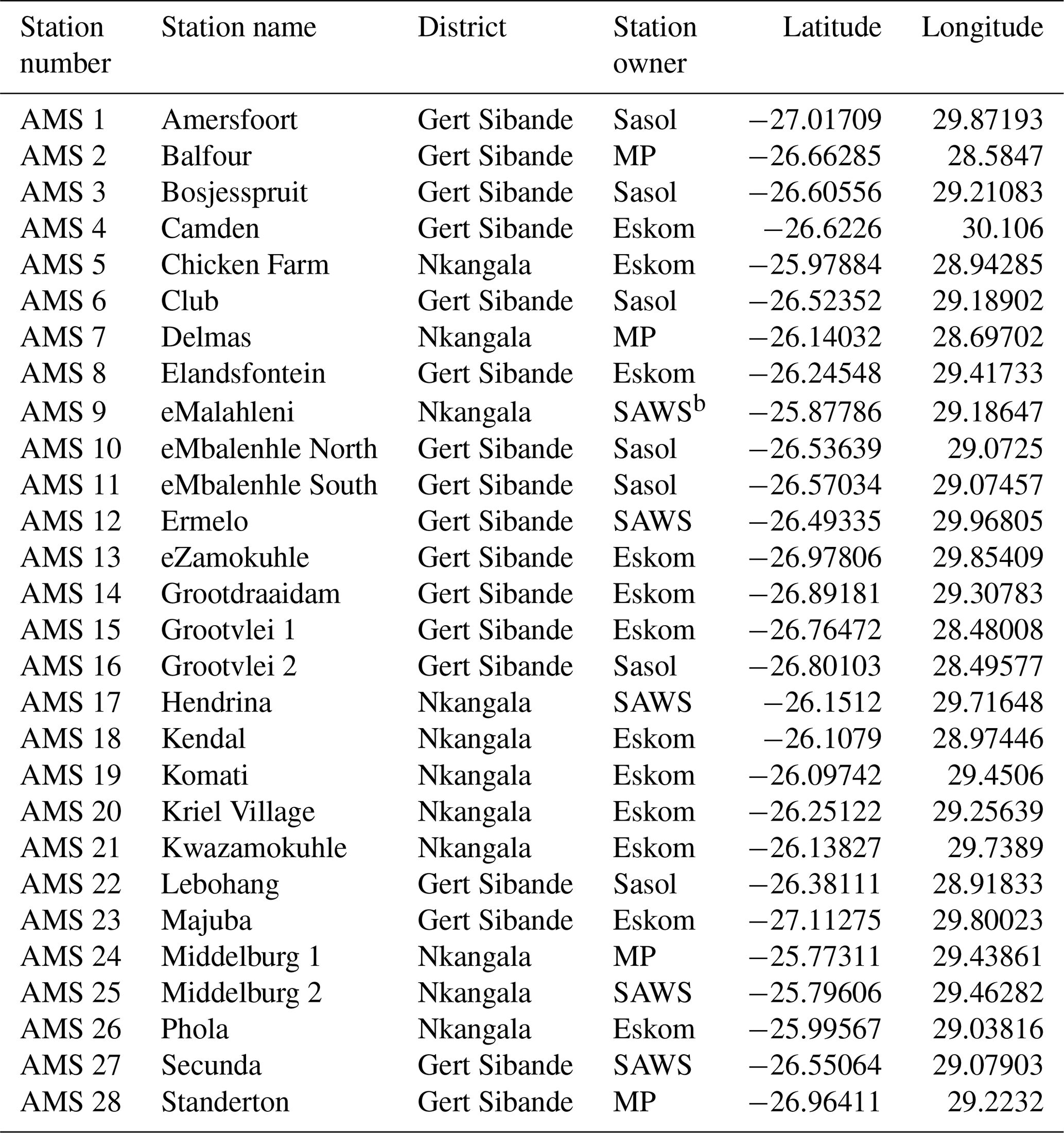
a Information was sourced from the South African Air Quality Information System (SAAQIS). b South African Weather Service.
Table B1False-positive rates of outlier detection among the respective observations selected for perturbation, across 100 iterations in clean data using .
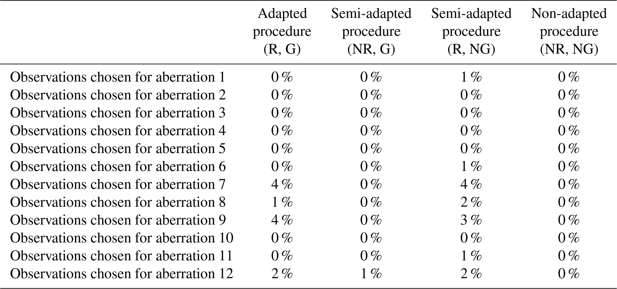
Table B2False-positive rates of outlier detection among the respective observations selected for perturbation, across 100 iterations in clean data using .
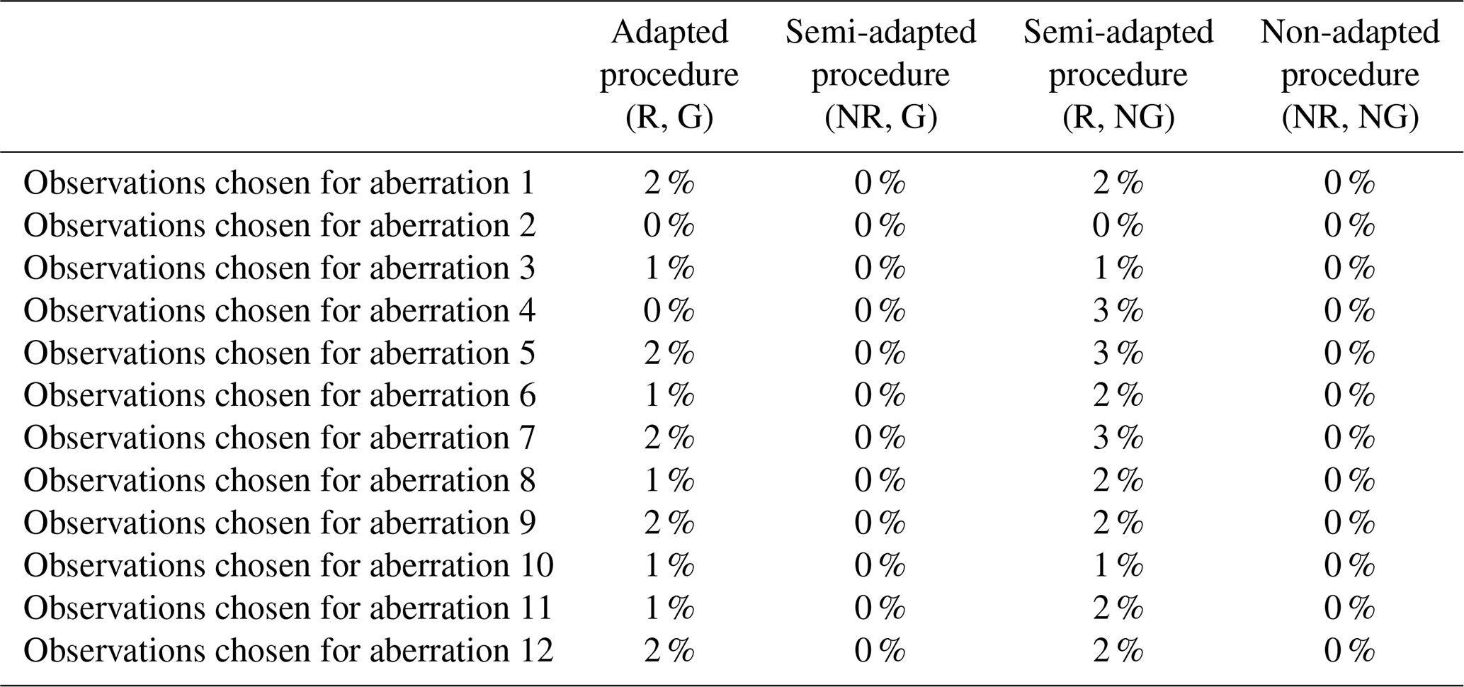
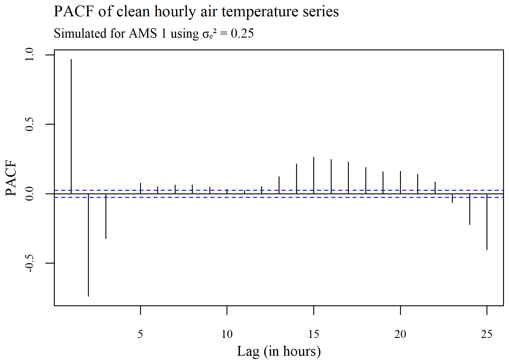
Figure C1Plot of the partial autocorrelation within a series of clean hourly air temperature data simulated for AMS 1, using .
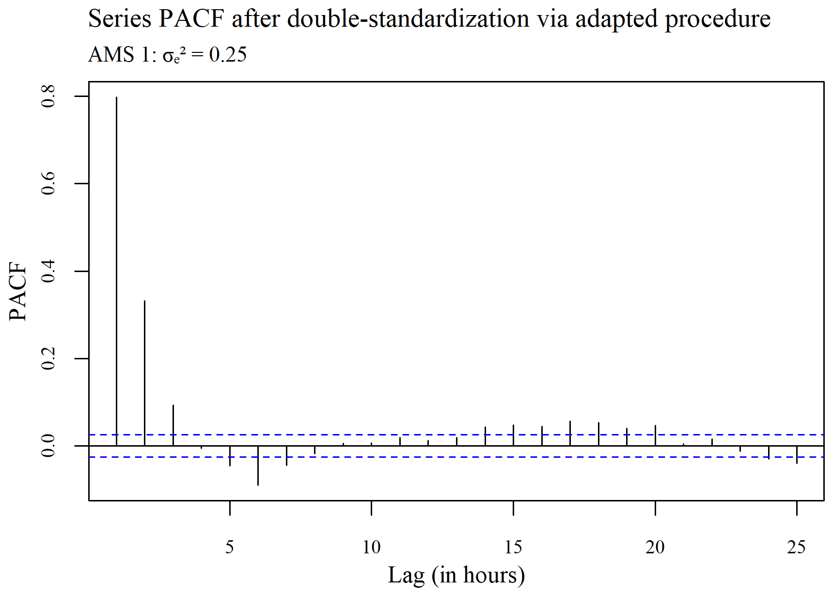
Figure C2Plot of the partial autocorrelation in the series, after double standardization of the data using the adapted procedure.
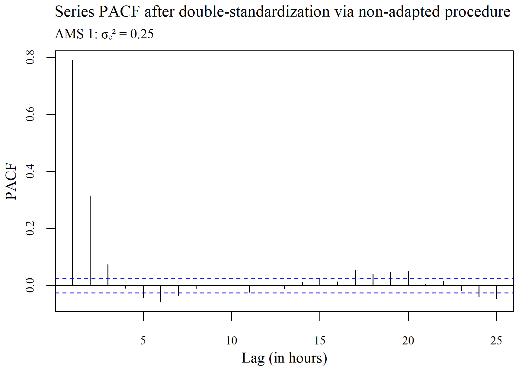
Figure C3Plot of the partial autocorrelation in the series, after double standardization of the data using the non-adapted procedure.
Table D1Results showing the success rates of the adapted double-standardization procedure (R, G) in detecting each aberration when a higher deviation threshold of h=5 was applied.
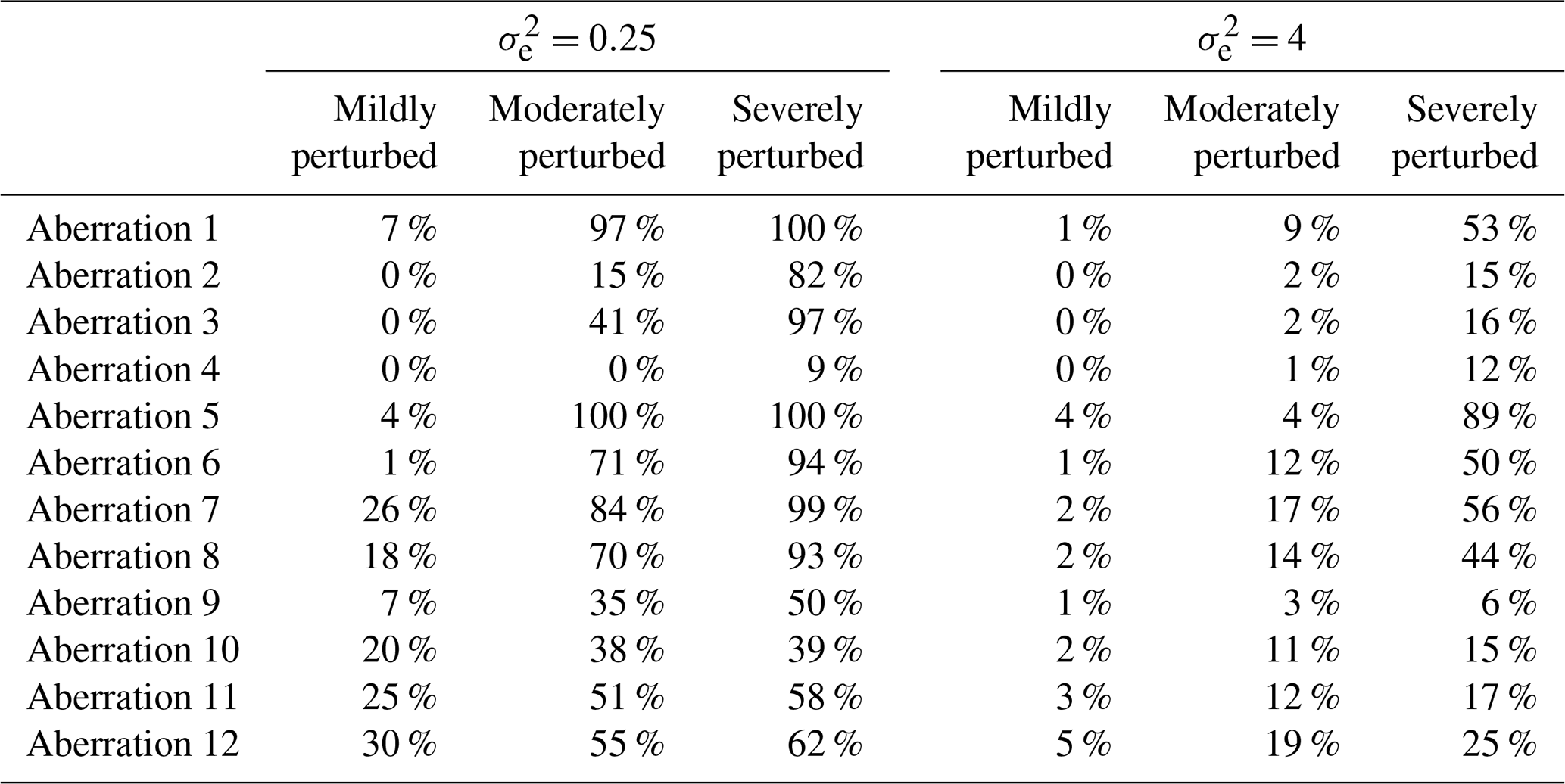
All of the data (both simulated and real) are available upon request from the corresponding author, together with the code used to conduct the simulation study and to generate the graphical analyses. The real data may alternatively be downloaded from the South African Air Quality Information System (https://saaqis.environment.gov.za/, last access 18 July 2023).
NDB: conceptualization, data curation, literature review, methodology, software, formal analysis, writing, visualization. TZ: methodology, supervision. RNN: data curation, supervision, writing – review and editing. DN: supervision, writing – review and editing.
The contact author has declared that none of the authors has any competing interests.
Publisher's note: Copernicus Publications remains neutral with regard to jurisdictional claims made in the text, published maps, institutional affiliations, or any other geographical representation in this paper. While Copernicus Publications makes every effort to include appropriate place names, the final responsibility lies with the authors.
The authors wish to thank the editor and referees for reviewing the article and improving its clarity. The authors also gratefully acknowledge the funding support received from the University Capacity Development Programme (UCDP). Special thanks are extended to Danielle Roberts for her contributions to the generation of certain figures.
This research has been supported by the University Capacity Development Programme (UCDP).
This paper was edited by Mark Risser and reviewed by two anonymous referees.
Almorox, J., Hontoria, C., and Benito, M.: Statistical validation of daylength definitions for estimation of global solar radiation in Toledo, Spain, Energ. Convers. Manage., 46, 1465–1471, https://doi.org/10.1016/j.enconman.2004.07.007, 2005.
Blazquez-Garcia, A., Conde, A., Mori, U., and Lozano, J. A.: A Review on Outlier/Anomaly Detection in Time Series Data, ACM Comput. Surv., 54, 56, https://doi.org/10.1145/3444690, 2021.
Campbell Scientific: Automatic Weather Stations (AWS) and Meteorologic Instruments: Worldwide standard for climate and boundary-layer meteorology, https://www.campbellsci.co.za/aws-meteorology (last access: 12 March 2025), 2024.
Lewinson, E.: Outlier Detection with Hampel Filter: How to implement the Hampel filter in Python from scratch, Towards Data Science, https://towardsdatascience.com/outlier-detection-with-hampel-filter-85ddf523c73d (last access: 12 March 2025), 2019.
Leys, C., Ley, C., Klein, O., Bernard, P., and Licata, L.: Detecting outliers: Do not use standard deviation around the mean, use absolute deviation around the median, J. Exp. Soc. Psychol., 49, 764–766, https://doi.org/10.1016/j.jesp.2013.03.013, 2013.
Linvill, D. E.: Calculating chilling hours and chill units from daily maximum and minimum temperature observations, HortScience, 25, 14–16, https://doi.org/10.21273/HORTSCI.25.1.14, 1990.
Luedeling, E., Caspersen, L., and Fernandez, E.: chillR: Statistical Methods for Phenology Analysis in Temperate Fruit Trees, R package version 0.76, CRAN, https://doi.org/10.32614/CRAN.package.chillR, 2024.
Lund, R., Hurd, H., Bloomfield, P., and Smith, R.: Climatological time series with periodic correlation, J. Climate, 8, 2787–2809, https://doi.org/10.1175/1520-0442(1995)008<2787:CTSWPC>2.0.CO;2, 1995.
Moore, D. S., McCabe, G. P., and Craig, B. A.: Introduction to the Practice of Statistics, 6, WH Freeman and Company, New York, ISBN 978-1-4292-1623-4, 2009.
Moreno-Tejera, S., Ramírez-Santigosa, L., and Silva-Pérez, M. A.: A proposed methodology for quick assessment of timestamp and quality control results of solar radiation data, Renew. Energy, 78, 531–537, https://doi.org/10.1016/j.renene.2015.01.031, 2015.
Owolabi, O., Okoh, D., Rabiu, B., Obafaye, A., and Dauda, K.: A median absolute deviation-neural network (MAD-NN) method for atmospheric temperature data cleaning, MethodsX, 8, 101533, https://doi.org/10.1016/j.mex.2021.101533, 2021.
Pearson, R. K.: Outliers in Process Modelling and Identification, IEEE T. Contr. Syst. T., 10, 55–63, https://doi.org/10.1109/87.974338, 2002.
Penn State Department of Meteorology: Subdividing the Mesoscale, https://learningweather.psu.edu/node/88 (last access: 12 March 2025), 2025.
Posio, J., Leiviskä, K., Ruuska, J., and Ruha, P.: Outlier Detection for 2D Temperature Data, in: IFAC Proceedings Volumes, 17th International Federation of Automatic Control World Congress, 6–11 July 2008, Seoul, South Korea, 1958–1963, https://doi.org/10.3182/20080706-5-KR-1001.00333, 2008.
SAAQIS – South African Air Quality Information System: SAAQIS, https://saaqis.environment.gov.za/ (last access: 18 July 2023), 2023.
Schlüter, S. and Kresoja, M.: Two preprocessing algorithms for climate time series, J. Appl. Stat., 47, 1970–1989, https://doi.org/10.1080/02664763.2019.1701637, 2020.
Spencer, J. W.: Fourier series representation of the position of the Sun, Search, 2, 172–175, 1971.
Van Poppel, M., Schneider, P., Peters, J., Yatkin, S., Gerboles, M., Matheeussen, C., Bartonova, A., Davila, S., Signorini, M., Vogt, M., Dauge, F. R., Skaar, J. S., and Haugen, R.: SensEURCity: A multi-city air quality dataset collected for 2020/2021 using open low-cost sensor systems, Sci. Data, 10, 322, https://doi.org/10.1038/s41597-023-02135-w, 2023.
Walker, A.: Some consequences of superimposed error in time series analysis, Biometrika, 47, 33–43, https://doi.org/10.2307/2332955, 1960.
Washington, B. J.: An Adapted VAR-EM Imputation of Climate Data and Statistical Downscaling of Temperature, Precipitation, and Solar Radiation in Puerto Rico, PhD thesis, University of Georgia, https://openscholar.uga.edu/record/6002 (last access: 3 September 2025), 2020.
Wickham, H.: ggplot2: Elegant Graphics for Data Analysis, Springer-Verlag, New York, ISBN 978-3-319-24277-4, 2016.
Wicklin, R.: The Hampel identifier: Robust outlier detection in a time series, SAS Blog, https://blogs.sas.com/content/iml/2021/06/01/hampel-filter-robust-outliers.html (last access: 15 March 2025), 1 June 2021.
Willmott, C. J. and Robeson, S. M.: Climatologically aided interpolation (CAI) of terrestrial air temperature, Int. J. Climatol., 15, 221–229, https://doi.org/10.1002/joc.3370150207, 1995.
Zewotir, T. and Galpin, J. S.: Evaluation of Linear Mixed Model Case Deletion Diagnostic Tools by Monte Carlo Simulation, Commun. Stat.-Simul. C, 35, 645–682, https://doi.org/10.1080/03610910600716795, 2007.
- Abstract
- Introduction
- Existing validation procedures for correlated series
- Proposed procedure for validation of strongly correlated series
- Evaluation of the new procedure by Monte Carlo simulation
- Application of the procedure to real data: a case study
- Conclusions
- Appendix A
- Appendix B
- Appendix C: Partial autocorrelation function plots for AMS 1 (in the case)
- Appendix D
- Code and data availability
- Author contributions
- Competing interests
- Disclaimer
- Acknowledgements
- Financial support
- Review statement
- References