Robust doubly censored Weibull modelling of NDVI-based burn-scar persistence in satellite time series

Burn-scar persistence in satellite imagery is treated as a lifetime process and modelled within a doubly censored Weibull framework arising from the finite temporal extent of satellite archives. Episodes may appear doubly censored in calendar time because the Landsat record spans a limited analysis window, so that for some pixels neither the true ignition time nor the full recovery are directly observed. On the persistence-time scale used for inference, incomplete episodes contribute as right-censored lifetimes within a unified likelihood formulation. A robust weighted-likelihood estimator with Huber-type influence weights downweights atypically long-lived scars without excluding any observations, thereby limiting the impact of outliers while preserving the central structure of the persistence distribution. The framework is applied to NDVI-based burn-scar persistence derived from Landsat surface-reflectance time series at Monitoring Trends in Burn Severity (MTBS) sampling locations within a large interior-Alaska fire scar, yielding a sample of 90 persistence episodes comprising fully observed and right-censored lifetimes. Weibull parameters are estimated under both maximum likelihood and weighted likelihood, with parametric bootstrap resampling used to obtain confidence intervals. Agreement between model-based and empirical survival behavior is assessed using Kaplan–Meier and Turnbull estimators and a Weibull probability plot. The fitted model indicates a median persistence of approximately 2.7–2.9 years and a 90th-percentile persistence of roughly five to six years, with the Weibull shape parameter consistently exceeding one, indicating an increasing recovery hazard over time. The proposed framework combines interpretability and robustness under censoring and generalizes naturally to other persistence-type environmental processes observed under incomplete monitoring.

1 Introduction

Quantifying how long burned landscapes remain spectrally visible in satellite imagery here termed burn-scar persistence is essential for understanding post-fire recovery and ecological resilience. Even with the continuity of modern Earth-observation archives, incomplete observation windows caused by cloud cover, orbital gaps and sensor outages often prevent full monitoring of fire-affected surfaces. The resulting temporal truncation leads to censoring, where the beginning or end of a persistence episode is unobserved, and thus complicates direct estimation of recovery durations. Similar difficulties arise in other persistence-type phenomena such as snow-cover longevity (Brown and Mote, 2009), floodwater retention (Sai Bhageerath et al., 2025) and orbital-debris decay (Ashruf et al., 2024), where observational incompleteness can bias lifetime inference (Gross and Clark, 1975). Post-fire vegetation dynamics in remote sensing have typically been described using spectral indices such as the Normalized Difference Vegetation Index (NDVI) and the Normalized Burn Ratio (NBR) derived from MODIS and Landsat imagery. Many studies fit smooth exponential or logistic trajectories to these indices to represent disturbance and recovery (Kennedy et al., 2010; Roy and Boschetti, 2009; Verbesselt et al., 2010), yielding visually intuitive but essentially deterministic descriptions. However, such trajectory-based models rarely account explicitly for statistical censoring or for radiometric noise in the underlying satellite observations (Kennedy et al., 2010; White et al., 2022) and may therefore underestimate actual recovery durations when recovery extends beyond the observation window. A probabilistic lifetime formulation, by contrast, can incorporate partial observation directly through survival-analysis principles, for example using nonparametric methods such as those of Kaplan and Meier (1958) and Turnbull (1976).

Within this probabilistic setting, the Weibull distribution provides a flexible model for persistence times: its shape parameter characterizes whether recovery accelerates or decelerates, while its scale parameter defines a characteristic duration (Murthy et al., 2004). Standard parameter estimation via maximum likelihood, however, is known to be sensitive to contamination and model deviations (Huber, 1981; Hampel et al., 1986; Huber and Ronchetti, 2009). Satellite data frequently contains outlying or mixed pixels arising from residual cloud, geolocation errors or misclassification, and these anomalies can distort the estimated hazard and bias ecological interpretation. To mitigate such effects, robust estimation methods have been proposed. The weighted-likelihood estimator was developed in the robustness literature to downweight discordant observations through case-specific likelihood weights (Markatou, 2000), and related minimum-distance and divergence-based approaches have been synthesized by Basu et al. (2011). The underlying principles of bounded influence and adaptive weighting were formalized in the robust M-estimation framework of Huber (1981) and Hampel et al. (1986) and further extended in later treatments (Huber and Ronchetti, 2009; Rousseeuw and Leroy, 1987). Building on these advances, the present study develops a Weibull lifetime model for burn-scar persistence under the doubly censored calendar-time structure induced by a finite observation window, estimated via a Huber-type weighted-likelihood estimator. The framework explicitly accounts for incomplete persistence episodes while moderating the impact of anomalous pixels, thereby improving stability without sacrificing interpretability. Using Landsat surface-reflectance time series at Monitoring Trends in Burn Severity (MTBS) sampling locations within a large interior-Alaska fire scar, with an analysis window from 2010 to 2018, the framework aims to combine statistical rigor with physical realism and to provide a unified tool for extracting meaningful persistence metrics from noisy, incomplete satellite observations.

2 Data and Observational Context

The analysis uses Landsat surface-reflectance time series extracted at Monitoring Trends in Burn Severity (MTBS) sampling locations within a large fire scar in interior Alaska (≈65.5° N, 145–146° W; USDA Forest Service and U.S. Geological Survey, 2024, MTBS; see also the MTBS methodological documentation in Fire Ecology). The MTBS points provide fixed 30 m reference locations inside the mapped burned area, allowing long NDVI histories to be reconstructed without spatial tracking. For each point, all available Landsat 5 TM, Landsat 7 ETM+, and Landsat 8 OLI observations from early 2000 onward were collected and converted to the Normalized Difference Vegetation Index (NDVI). Observations flagged as cloudy, heavily hazy, or snow-covered were discarded, leaving irregular but typically multi-decadal NDVI series for roughly one hundred burned pixels over the period 2000–2020. Burn-scar persistence was defined at each pixel as the time during which vegetation remained in a spectrally degraded post-fire state. To adapt this definition to local conditions, a “healthy vegetation” baseline was computed per pixel as the 80th percentile of its NDVI record. Percentile-based baselines and relative recovery thresholds are commonly used in Landsat time-series studies to define disturbance and recovery in a manner robust to interannual variability (e.g., Pickell et al., 2016; White et al., 2022; Smith-Tripp et al., 2024). A 5-point running median of NDVI was then used to identify disturbance and recovery. A burn episode was declared when the smoothed NDVI fell below 60 % of the baseline and remained below this threshold for several consecutive acquisitions; the first such crossing time was taken as the ignition date. Recovery was defined as the first subsequent time when smoothed NDVI returned to at least 85 % of the baseline, indicating that pre-fire greenness had effectively re-established. Similar relative-threshold definitions have been employed in post-fire recovery studies using Landsat time series, where recovery is operationally defined as return to a specified fraction of pre-disturbance spectral conditions (Pickell et al., 2016; White et al., 2022).

For each pixel, the dominant episode was taken as the longest contiguous interval below the burn threshold, with onset and recovery dates denoted by S_true and E_true. To mimic the finite monitoring windows typical of climate and satellite archives (Kennedy et al., 2010; White et al., 2022), a common analysis window was imposed across all pixels. In this study, [A,B] spans 1 January 2010 to 31 December 2018, capturing several post-fire growing seasons while remaining well within the Landsat record. The analysis window (2010–2018) was selected to represent a finite observation period and to ensure that the data exhibit a mixture of fully observed and censored persistence episodes. While the full Landsat record spans 2000–2020, using the entire period would lead to a higher proportion of fully observed episodes and fewer censored cases. In contrast, the selected window provides a more balanced combination of fully observed and right-censored observations, which is consistent with the censored lifetime framework adopted in this study. The choice of window is therefore intended to reflect incomplete monitoring conditions rather than to restrict the available data. Episodes that both ignite and recover within [A,B] contribute to fully observed lifetimes, with persistence $T=E_{\mathrm{true}}-S_{\mathrm{true}}$. Episodes that ignite within the window but remain spectrally degraded beyond B are right-censored, since only a lower bound on their persistence is observed. A small number of pixels are already in a degraded state at A and have not recovered by B; these give rise to doubly censored episodes whose ignition and recovery both lie outside the analysis window and whose persistence therefore exceeds the 3286 d span of [A,B]. After applying these steps, the final dataset consists of fully observed episodes, right-censored episodes, and a small number of long-lived doubly censored episodes, all expressed as persistence times in days. This configuration reflects key features of satellite-derived impact indicators – finite windows, irregular sampling, and moderate radiometric noise (Kennedy et al., 2010; Verbesselt et al., 2010; White et al., 2022) – and motivates a censored lifetime formulation in which complete and incomplete episodes are estimated jointly rather than discarding partially observed persistence intervals. Although the NDVI thresholds used to define disturbance (60 % of the pixel-specific baseline) and recovery (85 % of the baseline), as well as the 80th-percentile baseline itself, are necessarily heuristic, they are aligned with operational definitions of spectral recovery in Landsat-based disturbance studies. Simple sensitivity checks using alternative thresholds (e.g., 55 %–65 % for disturbance and 80 %–90 % for recovery) yielded qualitatively similar persistence distributions and Weibull parameter estimates, suggesting that the main conclusions are not driven by a single arbitrary choice of cut-off. Additional quantitative sensitivity analyses are provided in Appendix A (Table A2).

3 Conceptual Model of Persistence as a Doubly Censored Lifetime

Satellite archives rarely capture the full life cycle of ecological disturbances. In the case of NDVI-derived burn scars, some pixels are already in a degraded post-fire state when the analysis window opens, while others remain degraded when it closes. As a result, the complete trajectory from ignition to recovery is not always observed. This incomplete visibility naturally leads to censoring, a setting that parallels classical survival and reliability models (Gross and Clark, 1975; Lawless, 2003). We interpret burn-scar persistence as a lifetime variable. For each burned pixel, the persistence lifetime begins at the true onset of spectral degradation and ends when NDVI returns to a near-baseline level. Let S_true denote the true onset time of degradation and E_true the true recovery time. The persistence time is therefore $T=E_{\mathrm{true}}-S_{\mathrm{true}}$, T>0, measured in days from ignition to recovery. The satellite data are observed only within a fixed temporal window [A,B], defined in Sect. 2. Because this window does not necessarily cover the full interval [S_true,E_true], several censoring patterns arise in calendar time:

• Fully observed episodes: S_true≥A and E_true≤B. The entire persistence interval lies within the window, and the observed duration equals the true lifetime.

• Episodes beginning before the window: S_true<A and E_true≤B. Degradation has already started when observation begins.

• Episodes ending after the window: S_true≥A and E_true>B. Recovery occurs beyond the observation period.

• Episodes spanning the entire window: S_true<A and E_true>B. The pixel remains degraded throughout [A,B].

These censoring configurations are illustrated schematically in Fig. 1. In this paper, the term “doubly censored” refers to the calendar-time structure induced by the finite observation window [A,B], in which both ignition and recovery may lie outside the window. Statistical inference, however, is conducted entirely on the persistence-time scale T. On that scale, incomplete episodes do not generate interval-censored lifetimes; rather, they contribute as right-censored observations at their observed lower bound. The statistical model is formulated entirely in terms of the lifetime variable T, not the absolute calendar dates. When expressed on the T-scale, all incomplete episodes contribute as right-censored observations at their observed lower bound. In particular, episodes degraded throughout the window provide the information that $T>B-A$. Similarly, episodes that begin prior to A are left-censored in calendar time but provide right-censored information on the persistence-time scale. Thus, although the observation window induces patterns that may appear as left- or doubly censored in calendar time, the empirical likelihood for the present data involves only fully observed and right-censored persistence times. No interval-censored lifetimes arise on the T-scale in this application. The broader “doubly censored” perspective serves primarily to clarify how finite satellite archives generate incomplete lifetimes, whereas the statistical analysis itself operates on the persistence-time scale.

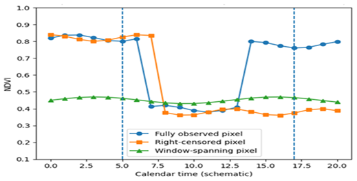
Figure 1 Example NDVI trajectories illustrating calendar-time censoring patterns. The vertical dashed lines mark the opening (A) and closing (B) dates of the satellite analysis window. Fully observed pixels recover within the window, right-censored pixels remain degraded beyond B, and doubly censored pixels are degraded throughout the entire observation window.

To model persistence, we assume that T follows a Weibull distribution with shape parameter b>0 and scale parameter θ>0. The cumulative distribution function is

$$\begin{array}{}\text{(1)}& F\left(t\right)=\mathrm{1}-e^{-{\left(\frac{t}{\mathit{\theta }}\right)}^b}\end{array}$$

and the corresponding density is

$$\begin{array}{}\text{(2)}& f\left(t\right)={\displaystyle \frac{b}{\mathit{\theta }}}{\left({\displaystyle \frac{t}{\mathit{\theta }}}\right)}^{b-\mathrm{1}}{e}^{-{\left(\frac{t}{\mathit{\theta }}\right)}^b}\end{array}$$

as in standard Weibull lifetime models (Murthy et al., 2004). For a fully observed persistence time t_i, the likelihood contribution is f(t_i). For a right-censored episode observed up to time c_i, the contribution is the survival probability 1−F(c_i). Accordingly, the likelihood used in this study is the standard right-censored lifetime likelihood familiar from survival analysis (Lawless, 2003; Turnbull, 1976). Framing burn-scar persistence as a censored lifetime process provides a transparent bridge between satellite data limitations and established statistical tools for incomplete time-to-event data. This formulation also enables principled extensions, including robust estimation and alternative distributional choices, which are developed in the following section. In Fig. 1, schematic NDVI trajectories illustrate fully observed, right-censored, and window-spanning episodes within the observation window [A,B].

In summary, although some episodes are left- or doubly censored in calendar time, the statistical inference is conducted entirely on the persistence-time scale, where incomplete episodes enter the likelihood as right-censored observations. This distinction ensures internal consistency between the conceptual description and the formal likelihood formulation.

4 Methodology

This section describes the estimation procedures used to model burn-scar persistence under censoring and to incorporate robustness through a weighted-likelihood estimator (WLE). The framework has three components: (i) formulation of the Weibull likelihood under general censoring; (ii) introduction of adaptive weighting to achieve robustness against outliers and model deviations; and (iii) quantification of uncertainty using parametric bootstrap resampling.

4.1 Weibull likelihood under general censoring

Let T_i denote the persistence time of the ith burned pixel, assumed to follow a Weibull distribution with shape b>0 and scale θ>0, with distribution and density given in Eqs. (1)–(2). In general, incomplete lifetime data may be represented by intervals (L_i,U_i) on the persistence-time scale, where $\mathrm{0}\le L_i<U_i\le \mathrm{\infty }$. Here, (L_i,U_i) denotes the lower and upper bounds within which the true persistence time T_i is known to lie under the censoring mechanism. In other words, the available data implies only that $T_i\in (L_i,U_i)$. When the episode is fully observed, the bounds coincide at the exact lifetime, so that $L_i=U_i=T_i$. Fully observed episodes satisfy $L_i=U_i=T_i$; pure left-censoring arises when L_i=0 and U_i<∞; pure right-censoring corresponds to L_i<∞ and U_i=∞; and interval-censored observations have $\mathrm{0}<L_i<U_i<\mathrm{\infty }$ (Lawless, 2003; Turnbull, 1976). In the MTBS application, although some episodes appear doubly censored on the calendar-time axis (Sect. 3), the statistical analysis is conducted on the persistence-time scale. On that scale, incomplete episodes contribute as right-censored observations at their observed duration. In particular, pixels degraded throughout [A,B] provide the information that $T>B-A$ and enter the likelihood as right-censored observations. Let ${\mathit{\delta }}_i^{\mathrm{obs}}$, ${\mathit{\delta }}_i^L$, ${\mathit{\delta }}_i^R$, and ${\mathit{\delta }}_i^I$ denote indicators for fully observed, left-censored, right-censored, and interval-censored observations, respectively, satisfying ${\mathit{\delta }}_i^{\mathrm{obs}}+{\mathit{\delta }}_i^L+{\mathit{\delta }}_i^R+{\mathit{\delta }}_i^I=\mathrm{1}.$ The general censored log-likelihood is

$$\begin{array}{}\text{(3)}& \begin{array}{rl}\mathrm{\ell }(b,\mathit{\theta })& =\sum _{i=\mathrm{1}}^n\left[{\mathit{\delta }}_i^{\mathrm{obs}}\log f\right(T_i;b,\mathit{\theta })+{\mathit{\delta }}_i^L\log F(U_i;b,\mathit{\theta })\\ & +{\mathit{\delta }}_i^R\log S(L_i;b,\mathit{\theta })\\ & +{\mathit{\delta }}_i^I\log \mathit{\left\{}F\right(U_i;b,\mathit{\theta })-F(L_i;b,\mathit{\theta }\left)\mathit{\right\}}],\end{array}\end{array}$$

where F and $S=\mathrm{1}-F$ denote the Weibull distribution and survival functions. In the empirical analysis below, only fully observed and right-censored persistence times arise on the lifetime scale, so the likelihood reduces to contributions of the form f(t_i) and S(c_i). Consequently, no interval-censored lifetimes arise in the MTBS application, and Eq. (3) simplifies accordingly. Maximizing ℓ(b,θ) yields the ordinary maximum-likelihood estimator (MLE), which is efficient under correct specification but can be sensitive to contamination and model deviations.

4.2 Weighted-likelihood formulation

To improve robustness, we adopt a weighted-likelihood approach following Markatou (2000) and the divergence-based framework of Basu et al. (2011). Each observation is assigned a weight $w_i\in [\mathrm{0},\mathrm{1}]$ that moderates its influence according to its agreement with the current fitted model. The weighted log-likelihood is

$${\mathrm{\ell }}_{\mathrm{W}}(b,\mathit{\theta })=\sum _{i=\mathrm{1}}^n{w}_i{\mathrm{\ell }}_i(b,\mathit{\theta }),$$

where ℓ_i(b,θ) denotes the individual contribution in Eq. (3).

Deviance-type residuals

Weights are constructed from standardized deviance-type residuals based on model-implied cumulative probabilities.

Define

$$u_i=\left\{\begin{array}{ll}F(T_i;b,\mathit{\theta }),& \text{if fully observed},\\ U_i,U_i\sim \mathrm{Uniform}\left(F\right(L_i;b,\mathit{\theta }),\mathrm{1}),& \text{if right-censored},\end{array}\right.$$

so that right-censored observations use randomized quantile residuals (Dunn and Smyth, 1996). The residual is obtained via the normal-score transformation, $r_i^{\left(\mathrm{0}\right)}={\mathrm{\Phi }}^{-\mathrm{1}}\left(u_i\right)$, where Φ⁻¹ is the standard normal quantile function. To achieve scale invariance, residuals are standardized using the median absolute deviation (MAD),

$$r_i={\displaystyle \frac{r_i^{\left(\mathrm{0}\right)}}{\mathrm{MAD}\left(r^{\left(\mathrm{0}\right)}\right)}}.$$

A Huber-type weight function (Huber, 1981; Huber and Ronchetti, 2009) is then applied

$$\begin{array}{}\text{(4)}& w_i=\left\{\begin{array}{ll}\mathrm{1},& \mid r_i\mid \le c,\\ \frac{c}{\mid r_i\mid },& \mid r_i\mid >c,\end{array}\right.\end{array}$$

where c>0 is a tuning constant controlling the bias–robustness trade-off.

Iterative algorithm

The weighted-likelihood estimator (WLE) ${\widehat{\mathit{\theta }}}_{\mathrm{W}}=\left({\widehat{b}}_{\mathrm{W}}{\widehat{\mathit{\theta }}}_{\mathrm{W}}\right)$ is obtained by:

• Initializing at the MLE.

• Computing residuals and updating weights.

• Maximizing ℓ_W(b,θ).

• Repeating until successive updates change by less than 10⁻⁶.

• When all weights equal one, the procedure reduces to the MLE.

4.3 Data-driven choice of the tuning constant

The tuning constant c governs the strength of downweighting. Rather than fixing it a priori, we adopt a data-driven selection rule. Let ${\widehat{F}}_{\mathrm{NP}}$ denote a nonparametric estimator of the persistence-time distribution (Kaplan–Meier or Turnbull, depending on the censoring structure), and let ${\widehat{F}}_{\mathrm{W},c}$ denote the Weibull distribution fitted via WLE with tuning constant c. For candidate values $c_{\mathrm{1}},\mathrm{\dots },c_M$, define

$$\begin{array}{}\text{(5)}& D\left(c\right)=\underset{\mathrm{0}}{\overset{\mathit{\tau }}{\int }}{\left\{{\widehat{F}}_{\mathrm{W},c}\left(t\right)-{\widehat{F}}_{\mathrm{NP}}\left(t\right)\right\}}^{\mathrm{2}}\mathrm{d}t\end{array}$$

where τ is a high quantile (e.g., the 95th percentile) of ${\widehat{F}}_{\mathrm{NP}}$. The selected constant is $\widehat{c}=\arg \underset{c\in \mathit{\{}{c}_{\mathrm{1}},\mathrm{\dots },c_M\mathit{\}}}{min}D\left(c\right)$ The selection rule is heuristic rather than likelihood-based, as it does not maximize a parametric criterion. Instead, it aims to balance robustness and fidelity to the empirical survival curve over the well-informed central duration range. The squared-loss functional was chosen for transparency and numerical stability, providing a simple measure of global discrepancy while modestly penalizing larger deviations. The truncation point τ limits the influence of sparsely populated upper-tail regions, where censoring is heavy and nonparametric estimates are inherently variable. As shown in Sect. 5.4, parameter estimates remain stable across a reasonable range of tuning constants, indicating limited sensitivity to this choice. This criterion is analogous to minimum-distance fitting against the nonparametric distribution over its central support, thereby limiting the influence of extreme tail behavior.

4.4 Bootstrap confidence intervals

Uncertainty in (b,θ) is assessed using parametric bootstrap resampling. For each of B=1000 replications, a synthetic dataset is generated from the fitted robust Weibull model $\left({\widehat{b}}_{\mathrm{W}},{\widehat{\mathit{\theta }}}_{\mathrm{W}}\right)$, preserving the observed censoring pattern. Specifically, lifetimes $T_i^{\ast }$ are generated from the fitted model and combined with the original censoring times C_i to form

$$T_i^{\mathrm{obs},*}=min(T_i^{*},C_i),{\mathit{\delta }}_i^{*}=\mathbf{1}(T_i^{*}\le C_i).$$

The weighted-likelihood algorithm with tuning constant $\widehat{c}$ is then applied to each bootstrap sample. Percentile-based 95 % confidence intervals are obtained from the empirical distribution of the bootstrap replicates. This approach captures sampling variability and the impact of censoring while avoiding reliance on information-matrix approximations under robustness adjustments (Efron and Tibshirani, 1993; Huber and Ronchetti, 2009).

4.5 Asymptotic properties

The WLE belongs to the class of divergence-based robust estimators for censored lifetime models (Markatou, 2000; Basu et al., 2011). Under standard regularity conditions for censored parametric models and bounded, smooth weight functions, the solution ${\widehat{\mathit{\theta }}}_{\mathrm{W}}$ to the weighted score equation

$$\begin{array}{}\text{(6)}& U_W\left(\mathit{\theta }\right)=\sum _{i=\mathrm{1}}^n{w}_i\left(\mathit{\theta }\right)u_i\left(\mathit{\theta }\right)=\mathrm{0}\end{array}$$

is consistent and asymptotically normal:

$$\sqrt{n}({\widehat{\mathit{\theta }}}_{\mathrm{W}}-{\mathit{\theta }}_{\mathrm{0}})\stackrel{d}{\to }{N}_{\mathrm{2}}(\mathrm{0},{\mathrm{\Sigma }}_{\mathrm{W}}),$$

where ${\mathrm{\Sigma }}_{\mathrm{W}}=J_{\mathrm{W}}^{-\mathrm{1}}{K}_{\mathrm{W}}{J}_{\mathrm{W}}^{-\mathrm{1}}$ is the usual sandwich covariance matrix based on the limiting sensitivity and variability matrices of the weighted score. When w_i≡1, this reduces to the classical MLE covariance structure. In practice, bootstrap-based inference is preferred here due to censoring and adaptive weighting. In the present application, rather than relying on closed-form expressions for Σ_W under censoring, inference is based on the parametric bootstrap described in Sect. 4.4.

5 Results and Interpretation

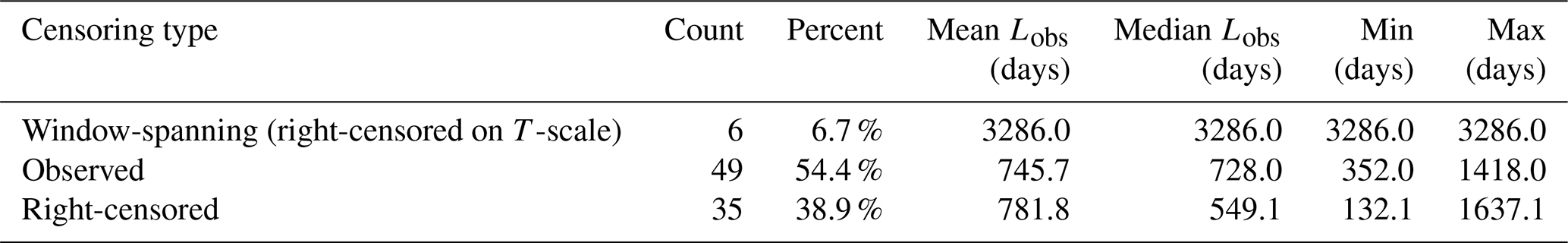
Table 1 summarizes the observed and censored burn-scar episodes in the MTBS sample (n=90). In the MTBS sample, 49 episodes (54 %) are fully observed and 35 (39 %) are right-censored on the persistence-time scale. An additional 6 episodes (7 %) remain degraded throughout the analysis window. These latter cases are doubly censored in calendar time but contribute as right-censored observations on the persistence-time scale. Nearly half of all episodes are therefore incomplete, underscoring the need for an explicit censored-lifetime formulation rather than relying on raw observed durations.

Table 1 Summary of observed and censored burn-scar episodes in the MTBS sample (n=90).

5.1 Model fit and parameter estimation

Fitting the Weibull model to the 90 MTBS episodes yields stable parameter estimates under both maximum likelihood (MLE) and weighted likelihood (WLE). Table 2 summarizes numerical results with bootstrap confidence intervals. Under both methods, the Weibull shape parameter exceeds one, indicating an increasing recovery hazard: the longer a scar persists, the more likely it is to recover in subsequent months. The scale parameter corresponds to persistence times on the order of two to three years, consistent with typical recovery trajectories in boreal and sub-arctic ecosystems (White et al., 2022; Smith-Tripp et al., 2024). The WLE primarily reduces sampling variability driven by a small number of very long-lived scars, including the window-spanning episodes discussed in Sect. 3, while leaving the overall recovery timescale essentially unchanged. The robust estimator produces slightly more stable estimates of the median and upper quantiles but preserves the central tendency. Overall, the Weibull model provides a compact and interpretable summary of the persistence distribution.

Table 2 Weibull parameter estimates and selected quantiles (days).

5.2 Model selection and validation

To assess distributional adequacy, lognormal and gamma models were fitted under the same right-censored likelihood structure used for the Weibull model. In all cases, episodes that are doubly censored in calendar time were represented as right-censored persistence times with $T_i>B-A$, ensuring direct comparability of likelihood-based criteria across distributions. Table 3 reports log-likelihoods and information criteria. The lognormal model attains the smallest AIC and BIC values, followed by the gamma distribution, while the Weibull MLE performs slightly worse under these criteria. The WLE version yields somewhat larger AIC/BIC values due to the effective reduction in influence from downweighted observations, though overall model fit remains comparable. Although the lognormal distribution achieves the smallest information criteria, estimated median persistence times and upper-tail quantiles are broadly comparable across the three models (Table 3). We retain the Weibull family as the primary model because it provides a direct monotone hazard interpretation and integrates naturally with the robust weighted-likelihood framework under right-censoring. The estimated shape parameter consistently exceeds one (Table 2), indicating an increasing recovery hazard over time – a pattern that aligns with ecological expectations of post-fire regrowth. Given the similarity of central and upper-tail persistence estimates across all candidate distributions, the choice of the Weibull model is guided by interpretability and robustness rather than marginal differences in information criteria. Nonparametric survival curves (Kaplan–Meier and Turnbull) were compared with the fitted WLE–Weibull survival curve (Fig. 2). The robust Weibull curve closely follows both empirical estimators over the central duration range of approximately 500–1500 d, with only modest deviations in the tails where data are sparse.

Table 3 Information criteria for alternative models (n=90).

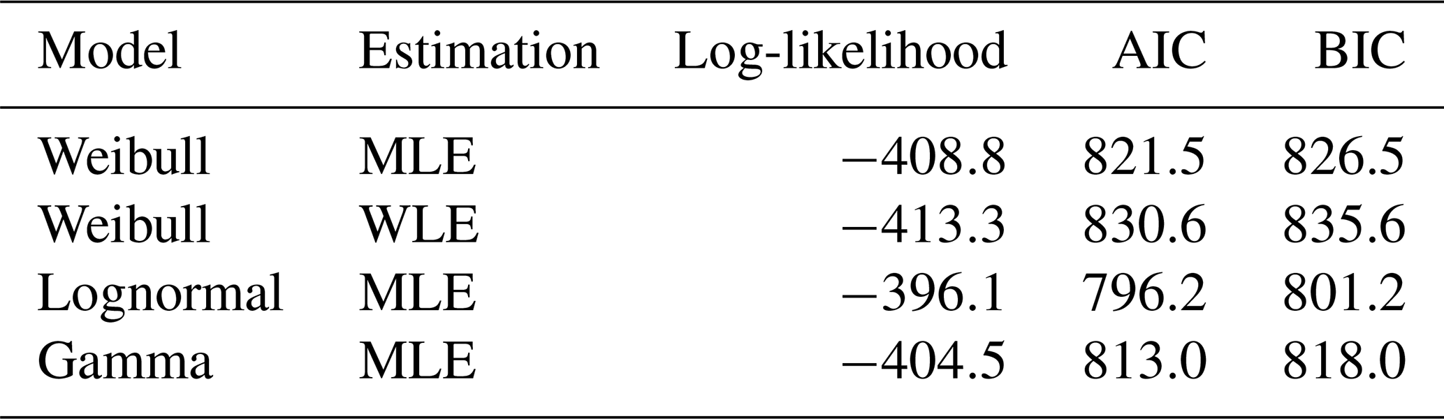
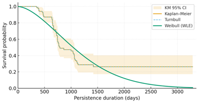
Figure 2 Nonparametric and parametric survival estimates for NDVI-based burn-scar persistence.

5.3 Robustness diagnostics: bootstrap and influence weighting

Robustness was examined using the bootstrap procedure described in Sect. 4.4. The bootstrap densities for the shape and scale parameters (Fig. 3a–b) exhibit narrower dispersion under the WLE than under the MLE, indicating that the robust procedure reduces variability driven by a small number of long-lived scars. Importantly, the central locations of the bootstrap distributions remain very similar under both estimators, suggesting that the WLE stabilizes inference without materially altering the central tendency. Figure 3c displays the Huber weight function at the selected tuning constant ($\widehat{c}\approx \mathrm{1.3}$). Episodes with $\mid r\mid \le \mathrm{1.3}$ receive full weight, while more discordant observations are progressively downweighted. Only a small fraction fall into the strongly downweighted region, indicating that most pixels exhibit broadly consistent recovery dynamics and that the robustness gains arise primarily from moderating a limited set of extreme cases.

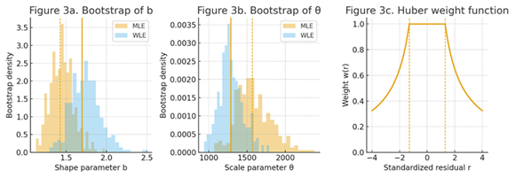
Figure 3 Bootstrap diagnostics and weighting function for the Weibull model: (a) bootstrap densities of the shape parameter b under MLE and WLE; (b) bootstrap densities of the scale parameter θ; (c) Huber weight function with cutoff at $\mid r\mid =\mathrm{13}$.

A Weibull probability plot for uncensored episodes is shown in Fig. 4. The empirical points display approximate linearity over the central quantile range, consistent with the Weibull specification. Departures are more visible in the lower and upper tails, where the number of uncensored observations is small and censoring is relatively heavy. Such deviations are consistent with finite-sample variability under tail sparsity and do not materially affect inference for the central portion of the persistence distribution, which drives the primary ecological interpretation. Taken together, Figs. 3 and 4 support the use of the WLE: it enhances numerical stability and mitigates the influence of extreme observations while preserving the primary structure of the persistence-time distribution.

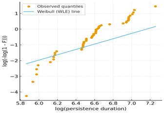
Figure 4 Weibull probability plot for uncensored burn-scar persistence episodes. Points are empirical quantiles of observed durations, and the line is the fitted WLE–Weibull model.

5.4 Sensitivity to the Huber tuning constant

To assess sensitivity to the Huber constant, the WLE–Weibull model was re-estimated for fixed values $c\in \mathit{\{}\mathrm{1.0},\mathrm{1.3},\mathrm{1.5}\mathit{\}}$. Table 4 summarizes the results. Across this range, the estimated shape and scale parameters – and the implied 10th, 50th, and 90th percentiles – vary only modestly. Median persistence remains close to approximately 2.7–2.9 years, and the 90th percentile lies between roughly 5.3 and 6.0 years. The data-driven choice $\widehat{c}$ falls within this range and yields estimates very close to those for c=1.3. This stability indicates that substantive conclusions about typical and extreme recovery times are not driven by the precise choice of the robustness parameter.

Table 4 Sensitivity of WLE–Weibull estimates to c.

6 Discussion

The results show that treating NDVI-based burn-scar persistence as a censored lifetime yields a coherent and physically meaningful description of recovery. In the MTBS sample, more than 40 % of episodes are incomplete either right-censored within the analysis window or degraded throughout it so that an approach based solely on raw observed durations would disregard a substantial portion of the available information. Within the Weibull family, the shape parameter summarizes whether the recovery hazard increases or decreases with time since fire, while the scale parameter defines a characteristic persistence horizon. Both quantities behave in an ecologically plausible manner, with median recovery times around 2.7–2.9 years and 90th-percentile durations of roughly five to six years. A key limitation of the present analysis is the modest sample size (n=90 episodes, of which only six span the entire observation window), which limits precision in characterizing the extreme upper tail of the persistence distribution and constrains exploration of more complex model structures. The definition of disturbance and recovery involves several NDVI thresholds: a pixel-specific baseline defined as the 80th percentile of the NDVI record, a 60 % drop below this baseline to flag disturbance, and an 85 % return threshold for recovery. These choices are necessarily heuristic but align with established practice in Landsat-based post-fire recovery studies. Sensitivity analyses with alternative thresholds (e.g., 55 %–65 % for disturbance and 80 %–90 % for recovery) yielded qualitatively similar persistence distributions and Weibull parameter estimates, indicating that the main findings are not driven by a single arbitrary specification. Methodologically, the weighted-likelihood estimator (WLE) provides clear robustness gains relative to standard maximum likelihood. Bootstrap diagnostics show that a small number of very long-lived scars inflate the variance of the MLE. Under the WLE, adaptive Huber weights moderate the influence of these episodes while leaving the bulk of the distribution essentially unchanged. This behavior is consistent with the theoretical properties of bounded-weight estimators, which stabilize likelihood curvature and reduce sensitivity to atypical observations while retaining the large-sample properties of likelihood-based inference. The data-driven selection of the tuning constant further enhances stability by adapting the robustness level to the observed lifetime distribution rather than fixing it a priori. Comparisons with alternative parametric forms reinforce these conclusions. Although the lognormal model attains the lowest AIC and BIC values and the gamma model performs competitively, neither offers the same combination of monotone hazard interpretation and well-developed robust censored-likelihood methodology available within the Weibull family. The WLE–Weibull fit closely follows the Kaplan–Meier and Turnbull curves over the central range of the data and yields a recovery hazard consistent with established patterns of post-fire regrowth. We therefore retain the Weibull family, estimated via WLE, as the primary modelling framework and regard the lognormal and gamma fits as benchmarks that confirm the overall stability of the substantive conclusions. Taken together, the results indicate that the proposed framework achieves three aims:

• i.

  It accommodates fully observed and right-censored persistence episodes within a unified lifetime model.

• ii.

  It embeds robustness directly into likelihood-based inference, addressing radiometric noise, misclassified pixels, and unusually persistent scars; and

• iii.

  It yields ecologically interpretable summaries of recovery timescales.

These features make the approach well suited to large or heterogeneous satellite datasets, where censoring and measurement noise are unavoidable and direct modelling of raw NDVI trajectories is often impractical. The same conceptual framework can be extended to other disturbance-and-recovery processes observed via remote sensing.

7 Conclusions

This study develops a robust lifetime-based framework for analyzing burn-scar persistence from NDVI time series, explicitly accommodating the censored structures that arise from the finite temporal extent of satellite archives. By modelling persistence as a Weibull lifetime and incorporating adaptive Huber weighting into the likelihood, the method combines a physically interpretable description of recovery with statistically stable estimation in the presence of noise, misclassified pixels, and unusually persistent scars.

Applied to 90 MTBS persistence episodes, the Weibull model captures the principal features of the recovery distribution, with median recovery times of approximately 2.7–2.9 years and substantially longer durations in the upper tail. The weighted-likelihood estimator stabilizes inference by reducing the influence of a small number of extreme episodes while preserving the central tendency of the distribution. Comparisons with nonparametric survival curves indicate that the robust Weibull fit aligns closely with the empirical lifetime structure over the central range of the data. Although the lognormal model attains slightly smaller AIC/BIC values and the gamma model performs competitively, neither offers the same combination of monotone hazard interpretation and an established robust censored-likelihood framework. In this sense, the Weibull–WLE formulation provides a balanced compromise between interpretability and robustness.

The framework is generic and can be extended to other satellite-based disturbance and restoration processes, such as vegetation browning, drought impacts, land-use transitions, and flood-recovery cycles. In the context of fire, the same methodology could be applied to major events outside interior Alaska – for example, the 2019–2020 Australian bushfires or large Amazonian drought fires – by adapting only the NDVI extraction and baseline definitions. Future work may incorporate spatial pooling across pixels, covariate effects such as climate forcing or fire severity, and hierarchical structures that combine multiple fire events within a unified statistical model. Overall, the proposed approach provides a principled and practical tool for extracting recovery timescales from incomplete and noisy remote-sensing observations, enabling more consistent characterization of post-fire ecosystem dynamics across diverse biomes and fire regimes.

Appendix A: Sensitivity of Parametric Inference

To examine the stability of the Weibull-based results, we carried out additional sensitivity analyses addressing two separate aspects of the modelling framework:

1. the robustness specification and the treatment of window-spanning episodes (Table A1), and

2. the preprocessing choices used to derive burn-scar persistence from the NDVI time series (Table A2).

Unless otherwise stated, all results are based on the same fixed set of 90 MTBS persistence episodes used in the main analysis.

A1 Sensitivity to Robustness Specification

We first evaluated how sensitive the results are to the choice of robustness tuning parameter in the weighted-likelihood estimator (WLE). The model was re-estimated for fixed values of the Huber constant $c\in \mathit{\{}\mathrm{1.0},\mathrm{1.3},\mathrm{1.5}\mathit{\}}$, covering a reasonable range of robustness levels.

In addition, as a diagnostic comparison, we re-fitted the Weibull model after excluding the six window-spanning episodes (i.e., pixels that remained degraded throughout the analysis window). This alternative specification results in n=84 observations.

The resulting parameter estimates and selected quantiles are reported in Table A1.

As shown in Table A1:

• the Weibull shape parameter remains strictly greater than one under all robustness settings,

• median persistence varies only moderately across specifications,

• upper-tail quantiles remain within the same multi-year range.

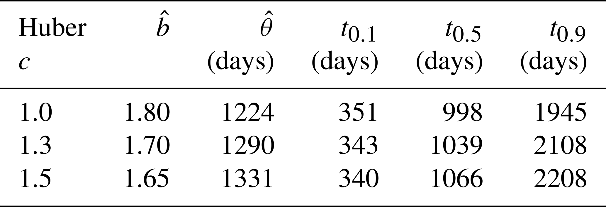
Excluding the window-spanning episodes reduces the influence of the extreme upper tail, as expected, but does not change the qualitative conclusion that recovery hazard increases over time. Overall, Table A1 indicates that the principal findings are not sensitive to the choice of robustness parameter nor to the inclusion of the longest-lived scars.

Table A1 Sensitivity of Weibull parameter estimates to the choice of Huber tuning constant and to the treatment of window-spanning episodes (n=90 unless otherwise stated).

A2 Sensitivity to NDVI Preprocessing Choices

We next evaluated the effect of the four main preprocessing decisions used to define burn-scar persistence:

• baseline percentile (75 %, 80 %, 85 %),

• disturbance threshold (55 %, 60 %, 65 % of the baseline),

• recovery threshold (80 %, 85 %, 90 % of the baseline),

• running-median window length (3 versus 5 observations).

For each alternative specification, persistence episodes were reconstructed from the original NDVI time series using:

• the same analysis window (1 January 2010–31 December 2018),

• the same dominant-episode selection rule, and

• the same fixed set of 90 MTBS sampling locations.

The Weibull model was then re-estimated using the same right-censored likelihood formulation as in the main analysis.

The results are presented in Table A2.

Several patterns are clear from Table A2:

• The Weibull shape parameter remains greater than one under every specification, indicating a consistently increasing recovery hazard.

• Median persistence remains on the order of several years for the main and nearby specifications.

• No alternative threshold choice produces a qualitatively different interpretation of recovery dynamics.

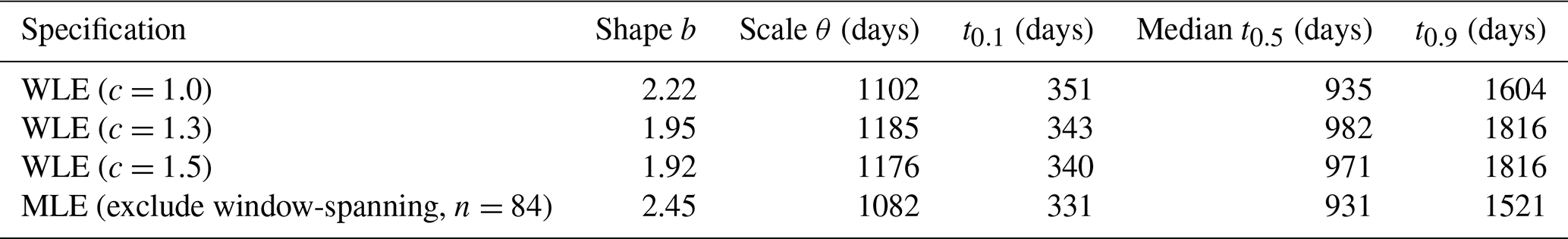
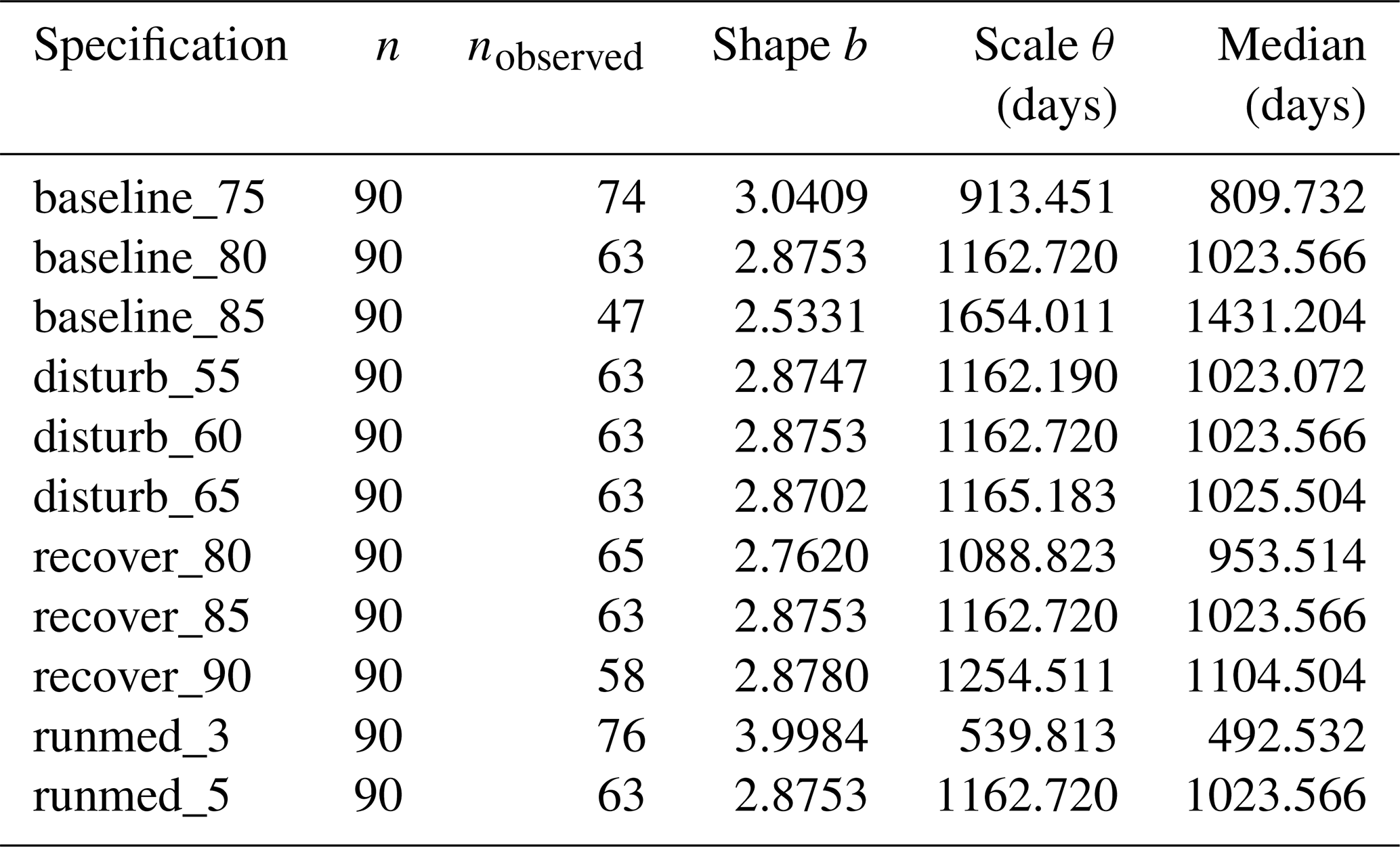
The disturbance threshold has almost no effect on the parameter estimates. In contrast, changes to the baseline and recovery thresholds produce gradual, monotonic shifts in estimated persistence timescales, which is expected since these parameters directly affect episode duration. The shorter smoothing window (k=3) yields shorter estimated durations, as reduced smoothing allows more rapid threshold crossings, but the increasing hazard interpretation remains unchanged. Taken together, the results in Table A2 confirm that the main conclusions of the study are not driven by any single threshold, percentile choice, or smoothing parameter.

Table A2 Sensitivity of Weibull maximum-likelihood estimates to alternative NDVI baseline percentiles, disturbance and recovery thresholds, and running-median window lengths (n=90).