Intelligent daily rainfall prediction for early warning using deep learning and satellite data: application to Bouaflé and Zuénoula stations, Ivory coast

Recurrent flooding in the Marahoué region, particularly in Bouaflé and Zuénoula, underscores the need for reliable and operational tools to anticipate hydrological risks and support early warning systems. This study presents a rainfall forecasting framework based on Long Short-Term Memory (LSTM) neural networks, integrating satellite-derived precipitation products and reanalysis-based atmospheric variables to predict daily rainfall at the Bouaflé and Zuénoula stations at t + 1, t + 3, and t + 7 d lead times. The performance of the LSTM model was systematically evaluated and compared with commonly used reference models, namely Random Forest (RF), Extra Trees (ET), and XGBoost (XGB), using standard statistical metrics (R², NSE, Pearson correlation coefficient R, normalized RMSE, and MAE). The results show that the LSTM model consistently outperforms the reference models across all forecasting horizons and at both study stations. At short and medium lead times (t + 1 and t + 3), LSTM exhibits strong predictive skill, with R² and NSE values exceeding 90 %, indicating an accurate representation of daily rainfall variability. Although performance decreases at the seven-day horizon due to increasing uncertainty and challenges in capturing extreme events, LSTM remains more robust than tree-based models, whose accuracy degrades markedly with increasing lead time. These findings confirm the relevance of LSTM-based approaches for rainfall forecasting and early warning applications in flood-prone regions. Future work will focus on integrating additional atmospheric predictors and applying advanced hyperparameter optimization techniques to improve long-term forecast reliability.

1 Introduction

Precipitation encompasses all meteoric waters, or hydrometeors, that fall to the Earth's surface, either in liquid form (rain) or solid form (snow, hail, sleet) (L'Hôte, 1993). In Africa, particularly in Ivory coast, precipitation consists exclusively of rainfall, whose intensity during the rainy season often causes severe flooding, leading to economic damages and loss of human lives. This hydroclimatic reality is well known in the Marahoué River Basin, where the localities of Bouaflé and Zuénoula are frequently affected by floods triggered by torrential rains during the rainy season, thereby threatening economic activities and human safety. Thus, accurate and quantitative near real-time rainfall forecasting can support the formulation of effective measures and help prevent human losses and material damages caused by flooding. The issue of rainfall prediction has long been a subject of scientific debate. Traditional approaches relying on statistical techniques have been used to quantitatively estimate rainfall. However, the complexity of rainfall processes, particularly their nonlinearity, makes prediction a challenging task (Wu and Chau, 2013). To address this, alternative methods have been developed to reduce nonlinearity, including singular spectrum analysis, empirical mode decomposition, wavelet analysis (Xiang et al., 2018; Gan et al., 2019), among other mathematical techniques. Nevertheless, the mathematical and statistical models employed often require high computational power (Singh and Borah, 2013) and may also be time-consuming.

Today, with advances in computer science, particularly artificial intelligence combined with hydrological modeling and meteorological satellite products integrated with efficient algorithms, new opportunities have emerged for achieving high-quality rainfall forecasts in near real time. Artificial intelligence, through machine learning, provides powerful algorithms capable of analyzing historical meteorological data to estimate future conditions, thus facilitating automated decision-making. Regarding satellite-derived meteorological products, the GPM IMERG program offers high-resolution temporal data suitable for global-scale monitoring, as demonstrated by recent studies (Simanjuntak et al., 2022). In fact, Simanjuntak et al. (2022) applied Long Short-Term Memory (LSTM), a deep learning algorithm, together with Random Forest (RF) models, to develop an early warning system for rainfall estimation in Indonesia, using data from the Himawari-8 geostationary satellite and GPM IMERG at 10 min intervals. Despite the great importance of having rainfall data at fine temporal resolutions, very few studies have been conducted in Ivory coast, and to date, no research has focused on near real-time rainfall prediction in any of its river basins. This study, therefore, complements previous works carried out in Ivory coast, particularly in the Marahoué Region, with the aim of improving existing approaches for the establishment of early warning systems for floods and rainfall forecasting. Its ambition is to explore deep learning techniques combined with GPM IMERG satellite data for near real-time rainfall prediction at different stations within the Marahoué River Basin.

2 Presentation of the study area

The study area considered in this research is located between longitudes 5°32^′ and 6°19^′ W and latitudes 6°45^′ and 7°36^′ N. It corresponds to a portion of the Marahoué River basin (Fig. 1) and encompasses the departments of Bouaflé and Zuénoula in central-western Ivory coast. The topography is characterized by gently undulating plateaus, with elevations ranging from 200 to 400 m, interspersed with low-lying areas that are regularly affected by seasonal flooding. The climate is of a tropical sub-equatorial type, featuring two rainy seasons (April–July and September–October) and two dry seasons (August and November–March) (Assoko, 2022). Average temperatures vary between 25 and 28 °C, while annual precipitation

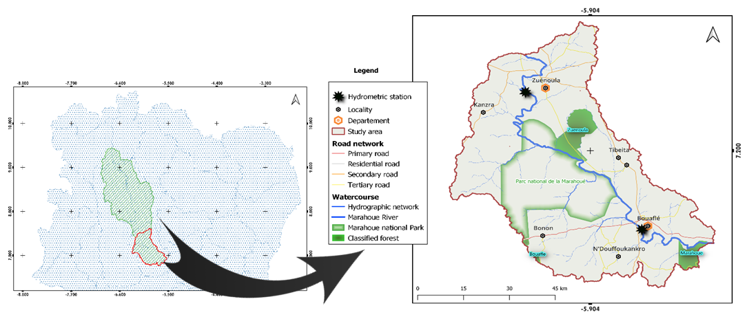
Figure 1 Location of the study area.

ranges from 1200 to 1600 mm. These climatic conditions, combined with a dense hydrographic network dominated by the Marahoué River, favor frequent flooding, particularly impacting agricultural zones and riverside communities. Geologically, the region rests on granitoid formations and Birimian series (Tagini, 1971; Kouamé et al., 2017). Economic activities, as highlighted by Peltre-Wurtz and Steck (1979) and Dje Bi (2015), are mainly centered on subsistence agriculture (yam, cassava, rice, maize), cash crops (coffee, cocoa), livestock farming (cattle, sheep, goats), and artisanal gold mining, which is particularly active in the Bouaflé department (Denis, 2016; Kouadio et al., 2018). However, the recurring floods severely disrupt production systems, increase the vulnerability of rural communities, and pose significant challenges for land use planning and territorial management.

3 Data and Materials

The data used in this study comprise both satellite-based climatic data and in-situ observations. Ground-based rainfall measurements were provided by the Airport, Aeronautical, and Meteorological Operations and Development Company (SODEXAM). The rainfall database covers daily records from 1 January 1961 to 31 December 2022 for the 10 operational stations in the Marahoué watershed (Bouaflé, Dianra, Kani, Kébi, Kongasso, Mankono, Morondo, Sarhala, Worofla, and Zuénoula). Special attention was given to the Bouaflé and Zuénoula stations, which served as the primary sites for the study. The historical records from these two stations include gaps, with missing data rates ranging from 7.29 % to 8.04 %. In addition, airborne data were collected from GPM IMERG and MERRA-2. GPM IMERG is a precipitation algorithm maintained by NASA and JAXA (Zubieta et al., 2017) that generates a relatively long satellite-based rainfall record of more than 20 years, with high spatial resolution (0.1°) and a temporal resolution of approximately 30 min, covering the entire globe. GPM IMERG data, available at https://pmm.nasa.gov/data-access/downloads/ (last access: 5 March 2024), were compiled at three-hour intervals and then aggregated to daily resolution for the study period 2000–2024. These data were acquired and preprocessed using the Google Earth Engine (GEE) platform, a cloud-based computing environment dedicated to the management, processing, and analysis of large satellite and climate data repositories, in order to fill gaps in the in-situ rainfall time series. MERRA-2 (Modern-Era Retrospective analysis for Research and Applications, Version 2) provides a reanalyzed set of atmospheric data produced by the Goddard Earth Sciences Data and Information Services Center (GES DISC), affiliated with NASA's Goddard Space Flight Center (GSFC). This reanalysis integrates satellite observations, ground-based measurements, and numerical weather prediction models through data assimilation techniques to generate spatially and temporally consistent atmospheric fields. Several variables, including hourly mean temperatures at 2 m a.g.l., as well as essential atmospheric parameters such as 50 m wind, sea-level and surface pressure, and other atmospheric pressures (Molod et al., 2015), were aggregated to daily time steps over the period from 1 January 1983 to 28 April 2024. These data were collected via Google Earth Engine to complement the training dataset for the developed models.

4 Methodology and model development

The methodological approach adopted in this study (Fig. 2) is structured in two main steps: data preprocessing and the application of deep learning models to estimate near real-time rainfall. The first step involves data acquisition and preparation using Google Earth Engine (GEE) via Google Colab. The second step describes the implementation of the models for rainfall estimation, the identification of relevant variables, and the validation of the performance of the developed models.

Figure 2 Methodological framework for near real time rainfall forecasting.

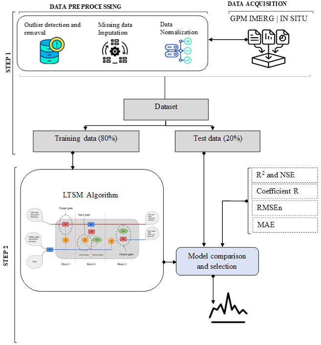
4.1 Data Preprocessing

The methodological framework implemented in this study is based on two successive and complementary steps: prior validation of the GPM IMERG satellite product, followed by quality control of the in-situ data at the scale of a network of 10 stations. Daily precipitation data from GPM IMERG were compared with ground-based observations over the 2000–2017 period for all 10 operational stations within the watershed. The correlation coefficient (R) was calculated for each station to assess the temporal consistency between the two data sources, and scatter plots were generated and fitted to provide visual validation. This step was intended solely to verify the overall reliability of the satellite product before its potential use as an auxiliary source during data correction.

Quality control was subsequently applied to the daily time series from the 10-station network, which provides the basis for the spatial consistency assessment. The stations of Bouaflé and Zuénoula, later used for model development, are part of this network but were not the only stations considered during the outlier detection phase. The adopted approach combines statistical quality control with spatial consistency verification, following recommended by Durre et al. (2010). At the individual station level, the interquartile range (IQR) method, according to Tukey (1977), was applied to identify observations exhibiting unusual deviations from the station-specific distribution. A value x was considered atypical if $x>Q_{\mathrm{3}}+\mathrm{1.5}\times$ IQR or $x<Q_{\mathrm{1}}-\mathrm{1.5}\times$ IQR, where Q₃ and Q₁ denote the first and third quartiles, respectively, and IQR $=Q_{\mathrm{3}}-Q_{\mathrm{1}}$

Given the potentially localized nature of precipitation processes, a spatial consistency check based on the median and the Median Absolute Deviation (MAD) was implemented to avoid removing physically plausible extreme events. For a given day j, an observation x_i,j at station i was compared to the network distribution and considered spatially inconsistent if $\left|x_{i,j}-{\stackrel{\mathrm{̃}}{x}}_j\right|>k\times {\mathrm{MAD}}_j$ where ${\stackrel{\mathrm{̃}}{x}}_j$ and MAD_j represent the network-wide median precipitation and the corresponding median absolute deviation for day j, respectively, with ${\mathrm{MAD}}_j=\mathrm{median}\left(\left|x_{i,j}-{\stackrel{\mathrm{̃}}{x}}_j\right|\right)$. The threshold k was analyzed for values between 2 and 3.5 in order to assess the sensitivity of detection rates and verify the robustness of the results.

Finally, an observation was classified as an outlier only if it was simultaneously atypical according to the IQR test and spatially inconsistent relative to the network. High-precipitation events that were spatially coherent were retained, even when exceeding statistical thresholds, to prevent the removal of meteorologically plausible extremes. Observations confirmed as erroneous were corrected or replaced only when necessary, using GPM IMERG as an auxiliary data. After applying this quality control protocol, the corrected dataset was used to develop predictive models specifically for the Bouaflé and Zuénoula stations. This dataset was normalized to a range between 0 and 1 using the formula in Eq. (1) as described by Hayder et al. (2023). This final operation performed on these data allows for an accelerated learning process (Jingwei et al., 2022).

$$\begin{array}{}\text{(1)}& \widehat{X}={\displaystyle \frac{X_i-\min \left(X\right)}{\max \left(X\right)-\min \left(X\right)}}\end{array}$$

where X_i is the input value, max(X) and min(X) refer, respectively, to the maximum and minimum values within the dataset X.

4.2 LSTM Model

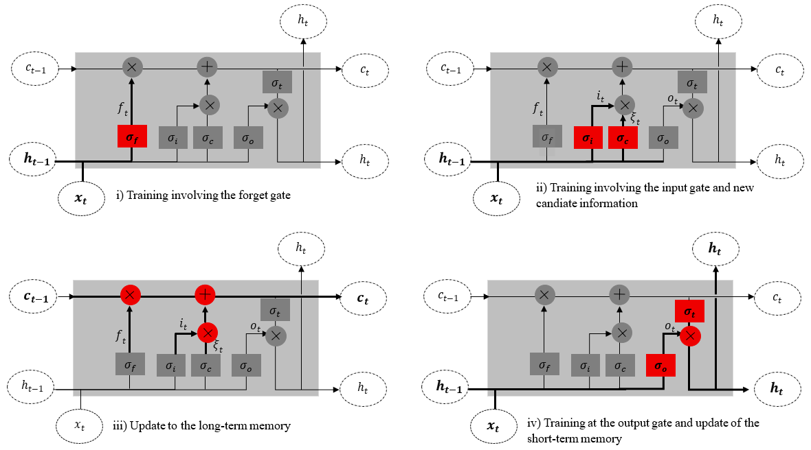
The Long Short-Term Memory (LSTM) model constitutes an advanced architecture of the traditional Recurrent Neural Network (RNN), initially proposed by Hochreiter and Schmidhuber (1997) to address the intrinsic limitations of standard RNNs, particularly their difficulty in capturing long-term dependencies and retaining information across extended sequences (Le et al., 2019). Its originality lies in the integration of specific components, referred to as gates, which regulate the selective transmission, storage, and forgetting of information, thereby enabling an efficient management of temporal dependencies (Gers et al., 1999). Unlike conventional RNNs, the LSTM relies on a sequence of recurrently connected memory cells, whose architecture enhances both the stability of the learning process and the accuracy of predictions (Hayder et al., 2023). The operational mechanism of the LSTM is schematically represented in Fig. 3, adapted from Zhao and Obonyo (2020). According to these authors, the LSTM includes two forms of memory: Long-term memory (c_t): information retained over time, stored in the cell state at time t; Short-term memory (h_t): information used immediately to perform the current task, represented by the hidden state at time t. The LSTM model operates as follows:

• Forget gate f_t. The model first determines which information from the previous cell state c_t should be retained or forgotten, based on the newly received input data;

• Input gate i_t. It then identifies the candidate new information c_t to be added to the long-term memory;

• Cell state update c_t. The new cell state is updated by combining the retained portion of the previous state with the new candidate information, modulated by the forget gate and the input gate;

• Output gate o_t. Finally, the model decides which part of the updated cell state should be exposed as output through the hidden state h_t, guided by the output gate.

Figure 3 Operating process of the LSTM Model.

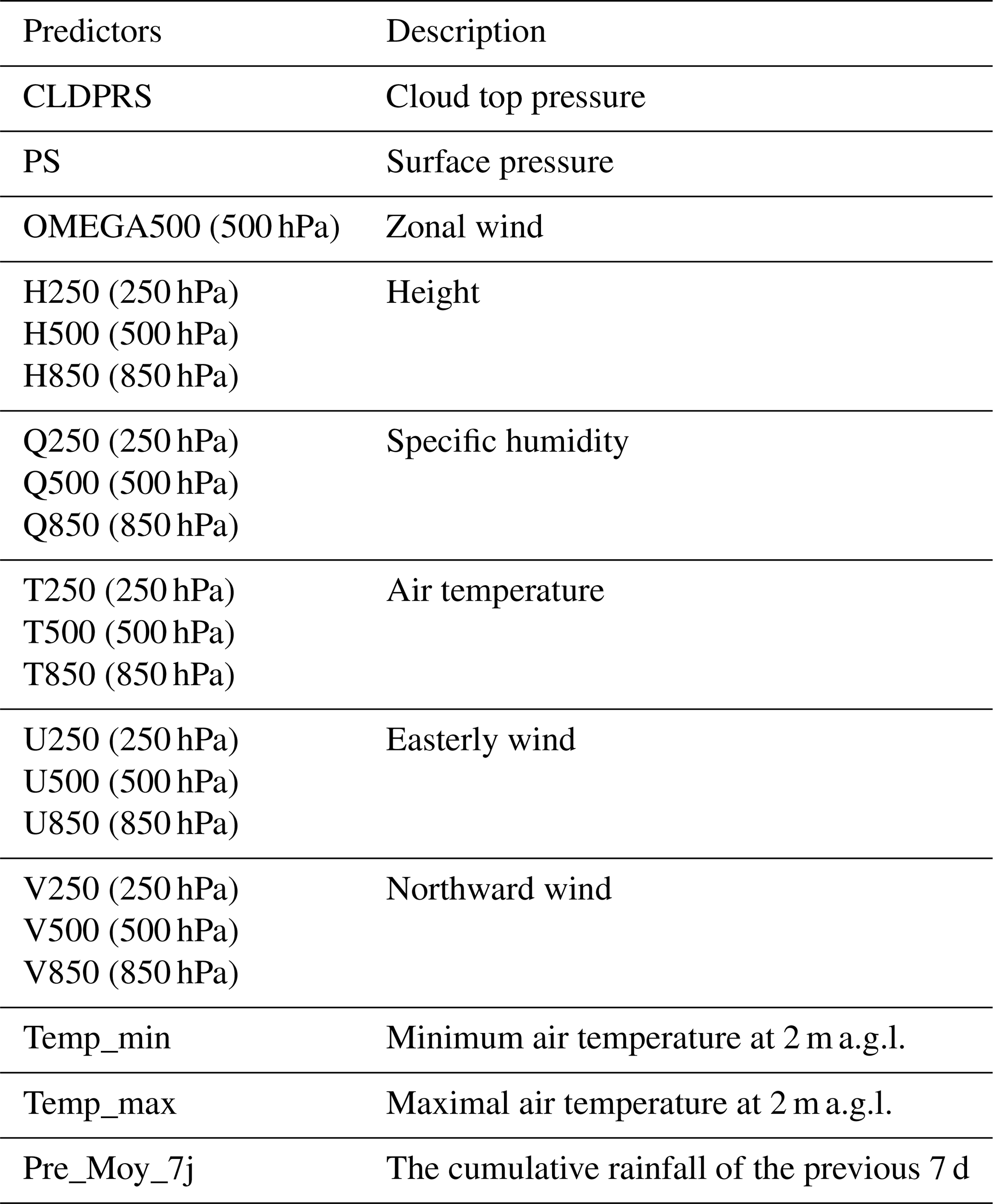
4.3 Identifcation of daily rainfall predictors and dataset

The selection of predictors was carried out based on their availability as well as those used in previous studies by Sagna (2021) and Endalie et al. (2022). Special attention was given to climatic factors, including temperature, atmospheric pressure, wind speed and direction, specific humidity, as well as sea surface temperature and temperature at 2 mȧ.g.l. Additionally, Integrated Water Vapor (IWV) data, although relevant for this type of study, were not available at a sufficient spatial resolution for the study area. A summary of these predictors is presented in Table 1. First, a correlation analysis was performed among the explanatory variables by computing the pairwise correlation matrix. Predictors exhibiting a correlation coefficient below 60 % with other predictors were retained, ensuring the selection of variables with minimal multicollinearity while preserving independent information for the LSTM modeling. Following this phase, the selected predictors were used as input variables for a Random Forest model to simulate daily precipitation. The relative importance of each predictor was then evaluated using the variable importance measures provided by the Random Forest algorithm. This analysis was used as a preliminary covariate selection step to identify the most informative predictors prior to training the LSTM model, thereby limiting redundant information, and improving model generalization. Variables with significant importance were considered relevant for daily precipitation forecasting due to their notable contribution to the model's accuracy.

Table 1 Predictors identified for rainfall forecasting.

4.4 Model construction and daily rainfall estimation

The methodological approach relied on the use of the Long Short-Term Memory (LSTM) model, which was implemented and optimized according to its architectural parameters within the PyTorch environment, widely used in deep learning applications (Xu, 2022). The input to the LSTM model consists of a three-dimensional tensor comprising the batch size, the input sequence length, and the number of input channels. The model output is also a tensor including the batch size and the sequence length, with a single output channel (1), corresponding to the predicted precipitation at the t + 1, t + 3, and t + 7 forecasting horizons (t expressed in days). Accordingly, three (3) distinct LSTM models were developed to perform the modeling at each of these forecasting horizons. To limit overfitting, several learning parameters were rigorously defined, including the number of hidden layers, the number of neurons per layer, the batch size, the number of iterations, the learning rate, and the temporal window length, which determines the data sampling interval. The optimization process consisted of adjusting one parameter at a time while keeping the others constant. For instance, the learning rate was initially set to 0.001, a value commonly adopted in the literature (Granet et al., 2018; Alavoine et al., 2024), and an automatic reduction of this rate was applied after five (05) epochs. The optimal value of each parameter was selected based on the minimization of the loss function and the improvement of fitting accuracy during the training process. When no improvement in the validation loss was observed after ten (10) epochs, an early stopping mechanism was activated. The Adam optimizer was used to update the network weights and biases in order to mitigate overfitting. All these steps were implemented using Python code executed on the Google Colab platform. To evaluate the performance of the LSTM model, it was compared with three reference models commonly used in hydrology, namely Random Forest (RF), Extra Trees (ET), and Extreme Gradient Boosting (XGB). The optimization of these reference models was performed using a grid search approach, in which the values of each hyperparameter were tested across a predefined set of values. Once optimized, these reference models were also used to predict precipitation at the t + 1, t + 3, and t + 7 forecasting horizons. After the model design phase, all developed models were trained on the normalized rainfall datasets from the Bouaflé and Zuenoula stations, using a supervised learning approach based on labeled input–output pairs. Cross-validation was incorporated to optimize model hyperparameters and to assess the robustness and generalization capability of the trained models. The dataset used in this study consists of daily observations spanning the period from 1 January 1984 to 28 April 2024, corresponding to a total of 15 094 time steps. For modeling and rigorous evaluation purposes, the data were divided into two distinct subsets. Observations from 1 January 1984 to 22 January 2020 (time steps 1–13 585) were used for model training, while those from 23 January 2020 to 28 April 2024 (time steps 13 586–15 094) were reserved for independent model validation.

4.5 Model validation

4.5.1 Statistical indicators

In order to rigorously assess the quality and predictive performance of the developed models, a set of widely recognized statistical indicators commonly employed in predictive modeling and machine learning was adopted. These metrics were used not only to evaluate model accuracy during training and validation phases, but also to guide hyperparameter tuning and determine the optimal model configuration. The evaluation framework incorporated three error-based measures: Root Mean Square Error (RMSE) (Willmott, 1981), Normalized Root Mean Square Error (RMSE_n) (Loague and Green, 1991), and Mean Absolute Error (MAE) (Kassam, 1977; Fouotsa Manfouo et al., 2023; Renteria-Mena et al., 2024), together with efficiency and correlation-based criteria, namely the Nash–Sutcliffe Efficiency (NSE), the coefficient of determination (R²) (Wright, 1921), and the Pearson correlation coefficient (R) (Pearson, 1909). During hyperparameter optimization, candidate models were compared using all these indicators. Particular emphasis was placed on RMSE as the primary selection criterion because of its sensitivity to large deviations, which is critical for daily rainfall modeling where extreme events strongly influence predictive reliability. MAE was also considered as a complementary metric, providing an assessment of the average magnitude of errors without disproportionately penalizing large deviations. When discrepancies occurred among the metrics, the configuration with the lowest RMSE was selected as the optimal model. MAE, NSE, and R² were used as complementary metrics to ensure consistent and acceptable model performance. These metrics were implemented in a Python environment, ensuring automated execution and consistent computation during both training and validation phases. The corresponding mathematical formulations of these indicators are presented below.

$$\begin{array}{}\text{(2)}& {\displaystyle }\mathrm{RMSE}=\sqrt{{\sum }_{i=\mathrm{1}}^N{\displaystyle \frac{{\left(\widehat{y_i}-y_i\right)}^{\mathrm{2}}}{N}}}\text{(3)}& {\displaystyle }{\mathrm{RMSE}}_n=\mathrm{100}\times {\displaystyle \frac{\mathrm{RMSE}}{\stackrel{\mathrm{‾}}{O}}}\text{(4)}& {\displaystyle }\mathrm{MAE}={\displaystyle \frac{{\sum }_{i=\mathrm{1}}^N\left|y_i-{\widehat{y}}_i\right|}{N}}\text{(5)}& {\displaystyle }{R}^{\mathrm{2}}\left(\mathrm{\%}\right)=\left(\mathrm{100}\right)\times \left[\mathrm{1}-{\displaystyle \frac{{\sum }_{i=\mathrm{1}}^N{\left(\widehat{y_i}-y_i\right)}^{\mathrm{2}}}{\sqrt{{\sum }_{i=\mathrm{1}}^N{\left(y_i-\stackrel{\mathrm{‾}}{y_i}\right)}^{\mathrm{2}}}}}\right]\text{(6)}& {\displaystyle }\mathrm{NSE}\left(\mathrm{\%}\right)=\left(\mathrm{100}\right)\times [\mathrm{1}-{\displaystyle \frac{{\sum }_{i=\mathrm{1}}^N{\left(y_i-{\widehat{y}}_i\right)}^{\mathrm{2}}}{\sqrt{{\sum }_{i=\mathrm{1}}^N{\left(y_i-\stackrel{\mathrm{‾}}{y}\right)}^{\mathrm{2}}}}}]\text{(7)}& {\displaystyle }\mathrm{R}\left(\mathrm{\%}\right)=\left(\mathrm{100}\right)\times \left[{\displaystyle \frac{{\sum }_{i=\mathrm{1}}^N\left(y_i-\stackrel{\mathrm{‾}}{y}\right)\left({\widehat{y}}_i-\stackrel{\mathrm{‾}}{\widehat{y}}\right)}{\sqrt{{\sum }_{i=\mathrm{1}}^N{\left(y_i-\stackrel{\mathrm{‾}}{y}\right)}^{\mathrm{2}}{\sum }_{i=\mathrm{1}}^N{\left({\widehat{y}}_i-\stackrel{\mathrm{‾}}{\widehat{y}}\right)}^{\mathrm{2}}}}}\right]\end{array}$$

where y_i is the observed data, ${\widehat{y}}_i$ is the predicted data, and N is the length of the dataset, $\stackrel{\mathrm{‾}}{y}$ is the mean of the observed data, and $\stackrel{\mathrm{‾}}{\widehat{y}}$ is the mean of the predicted data.

According to Hussain et al. (2023), a normalized RMSE (RMSE) lower than 10 % indicates excellent model performance, while a value between 10 % and 20 % reflects very good performance. When RMSE ranges between 20 % and 30 %, the model is considered moderately accurate, whereas values exceeding 30 % denote poor reliability. Furthermore, model performance improves as the MAE (Mean Absolute Error) approaches zero, which demonstrates higher predictive accuracy (Chicco et al., 2021). Regarding the coefficient of determination (R²) and the Nash–Sutcliffe Efficiency (NSE), values above 90 % characterize an excellent model, those between 80 % and 90 % a very satisfactory model, those between 60 % and 80 % a satisfactory model, while values below 60 % indicate poor performance (Bodian et al., 2012). Finally, a value of R greater than or equal to 80 reflects a very strong correlation between variables, a value between 50 and 80 indicates a strong correlation, whereas a value below 50 suggests a weak correlation.

4.5.2 Quality of the rainfall estimates

In addition to the statistical performance criteria, a residual analysis was carried out to further evaluate the quality of rainfall estimates generated by the best-performing model and to assess their consistency with observed field data. Residuals were computed as the difference between observed and simulated values (Bodian, 2011). A statistical evaluation was then performed following the recommendations of Lek et al. (1996). According to these authors, residual analysis involves verifying their stationarity with respect to the predicted variable and ensuring that their mean is statistically zero, which would indicate that the estimates are unbiased. Stationarity was examined through a graphical analysis of the residuals plotted against the model outputs. It was also deemed necessary to analyze the residuals according to classes of predicted values in order to evaluate potential variations with rainfall intensity. The distribution of residuals was assessed using the Kolmogorov–Smirnov test implemented in Python, with the following hypotheses: H0: the residuals follow a normal distribution and H1: the residuals do not follow a normal distribution. This test was performed to verify whether the residuals satisfy the normality assumption, which is part of the underlying assumptions of the model, and to identify potential deviations such as skewness or extreme values.

5 Results

5.1 Validation of GPM data and gap filling of in situ data

The Figs. 4 and 5 show the different scatter plots and the corresponding fittings performed for each station. The correlation coefficient was calculated, and a linear regression equation was determined.

Figure 4 Scatter plot of GPM and in situ rainfall at Bouaflé station (2000–2017).

Figure 5 Scatter plot of GPM and in situ rainfall at Zuenoula station (2000–2017).

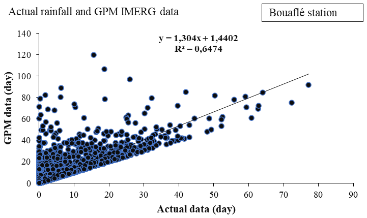
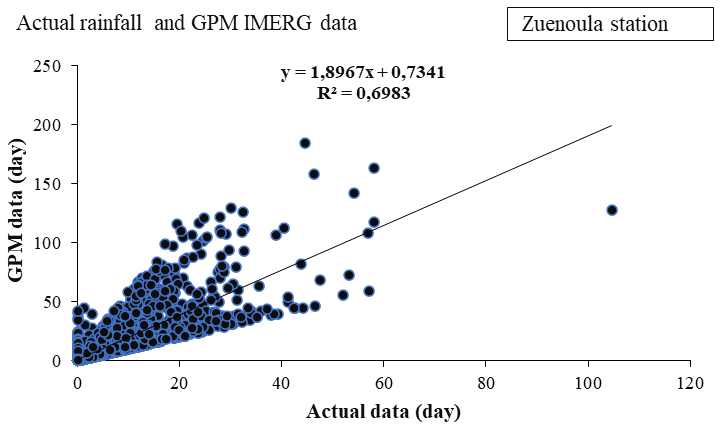
Figures 4 and 5 present scatter plots comparing daily rainfall estimates from the satellite-based GPM IMERG product with in situ rain gauge observations at the Bouaflé and Zuénoula stations, respectively. At the Bouaflé station (Fig. 4), a strong positive correlation is observed between the two datasets, with a correlation coefficient of 0.80, indicating that GPM IMERG reproduces approximately 80 % of the variability in the in-situ rainfall observations. Similarly, at the Zuénoula station (Fig. 5), the correlation coefficient reaches 0.83, reflecting a high level of consistency between satellite-based estimates and ground-based measurements. Overall, these results demonstrate that GPM IMERG rainfall estimates are in good agreement with in situ observations at both stations, capturing more than 80 % of the observed rainfall variability. Based on this level of agreement, GPM IMERG data were considered sufficiently reliable and were therefore used to replace missing values in the ground-based rainfall records prior to model development. The quality control, based on a combination of the interquartile range (IQR) test and a spatial consistency check applied to the network of ten stations in the Marahoué basin, identified 689 outliers out of a total of 29 510 observations from the Bouaflé and Zuénoula stations, representing 2.34 %. This relatively low percentage indicates a generally good data quality and is consistent with the proportions commonly reported in climatological studies. Observations confirmed as erroneous after spatial verification were corrected only when necessary, using the previously validated GPM IMERG estimates as an auxiliary source, while spatially coherent extreme events were retained.

5.2 Selection of significant variables

Figure 6 presents the correlation matrix for twenty-one (21) variables, namely CLDPRS, PS, OMEGA500, H250, H500, H850, Q250, Q500, Q850, T250, T500, T850, U250, U500, U850, V250, V500, V850, Temp_min, Temp_max, and Pre_Moy_7j. Analysis of this matrix (Fig. 6) reveals a clear division of the variables into two distinct groups. Group 1 includes variables with correlation coefficients below 0.60, namely Pre_Moy_7j, OMEGA500, U500, Q250, T250, V500, V850, T500, U850, U250, Q850, Q250, V250, and Temp_min. The remaining predictors, with correlation coefficients above 0.60, form Group 2, which was excluded from the dataset used for modeling. For the subsequent analysis, variables from Group 1 (Fig. 7) were selected as input features for the Random Forest model to assess their relative importance.

Figure 6 Pearson correlation matrix of all predictor variables.

Figure 7 Pearson correlation matrix of the selected predictor variables.

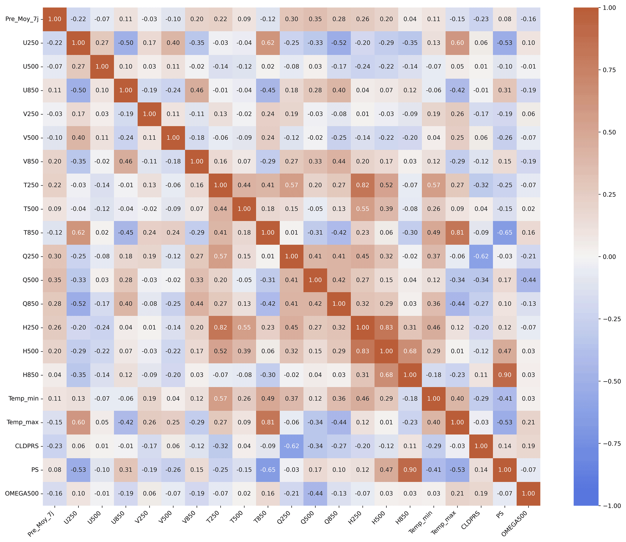
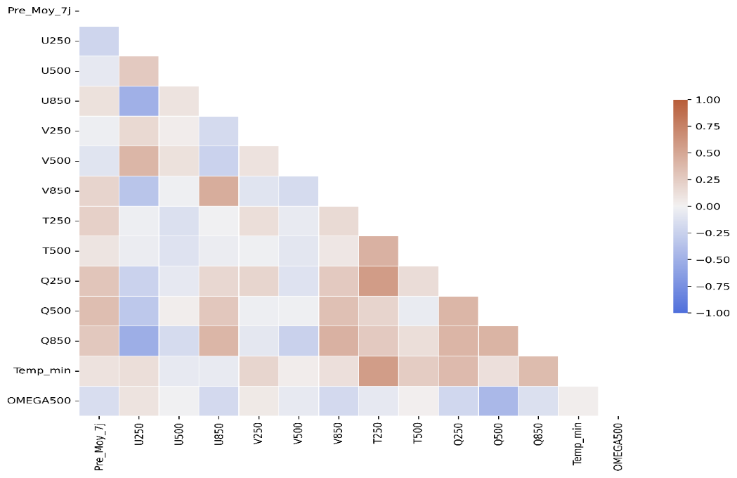
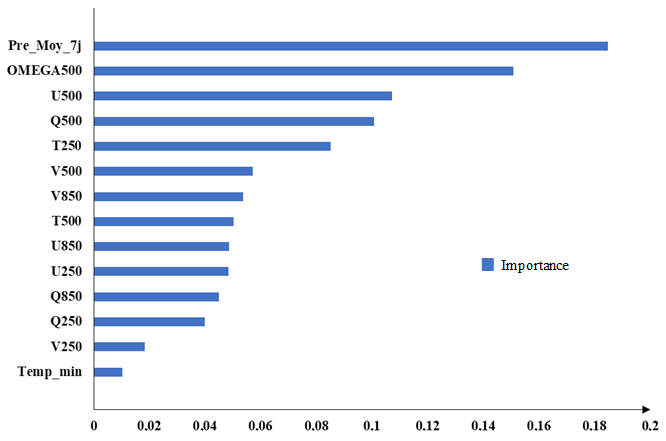
Figure 8 presents the importance levels of Group 1 variables as evaluated by the Random Forest algorithm. The analysis of this figure indicates that most variables in Group 1 had a considerable impact on the model, with significance scores ranging from 0.04 to 0.18, except for V250 and Temp_min, whose importance levels were below 0.04. To construct a set of predictors with an acceptable level of importance, only variables with importance scores greater than 0.04 were retained for daily rainfall forecasting, as they were considered significant for the study. These variables include Pre_Moy_7j, OMEGA500, U500, Q250, T250, V500, V850, T500, U850, U250, Q850, and Q250.

Figure 8 Variable importance according to the Random Forest algorithm.

5.3 Model performance

Before presenting the model performance results, it is important to note that all evaluation metrics are detailed in Sect. 4.5. The RMSE was used as the primary metric for selecting the optimal models, followed by normalized RMSE and MAE, while the R² and NSE coefficients were considered as complementary indicators to confirm the overall consistency of model performance.

5.3.1 Model optimization

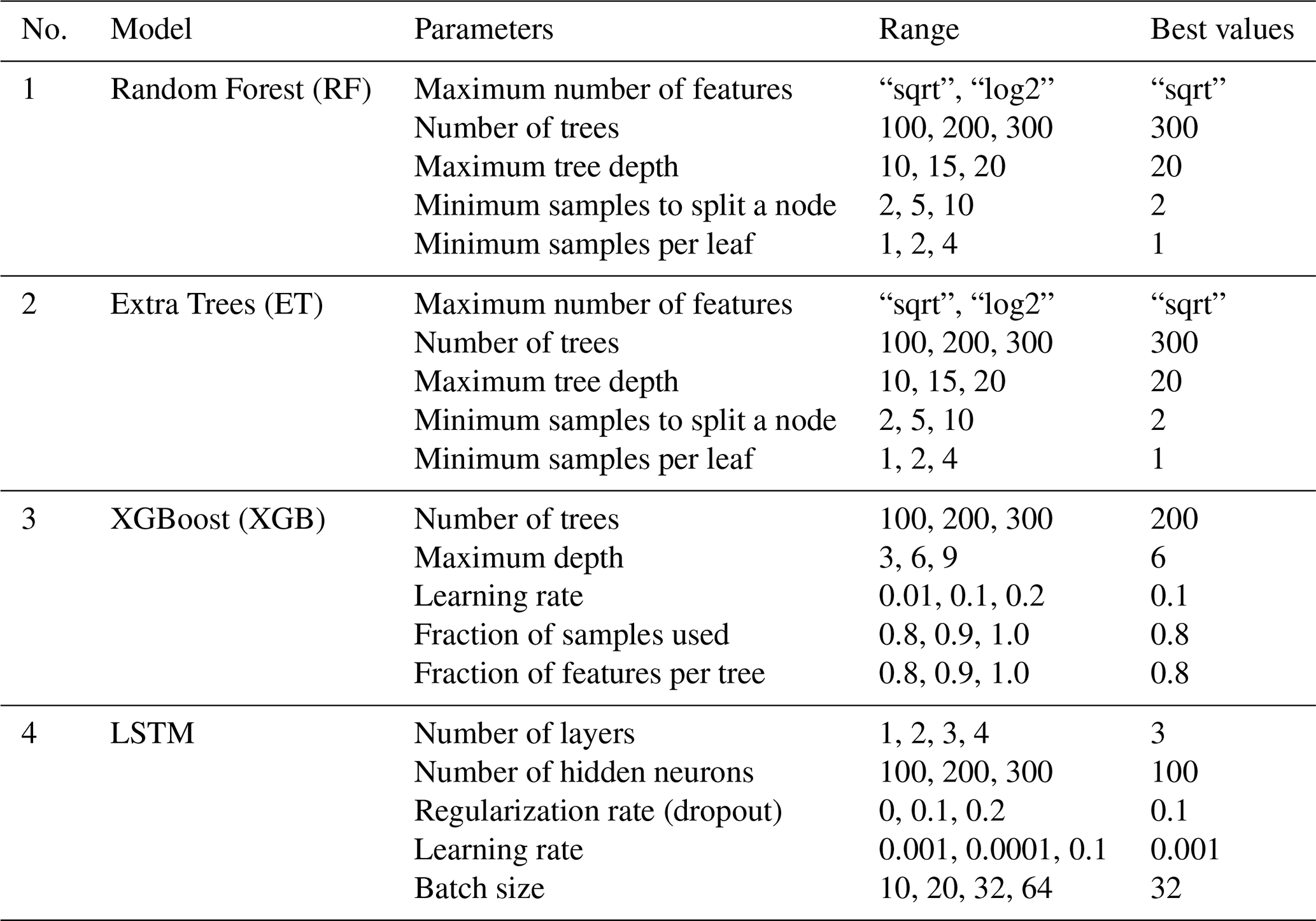
The developed models were optimized according to several hyperparameters (Table 2). For Random Forest (RF) and Extra Trees (ET), the maximum number of features was determined using the “sqrt” option for the max_features parameter. In this configuration, the number of candidate predictors randomly selected at each split is equal to the square root of the total number of input features ($\sqrt{p}$), where p denotes the total number of predictors. The models were configured with 300 trees and a maximum depth of 20, while all other hyperparameters were retained at their default settings, indicating consistency in modeling the complex relationships of rainfall processes. For XGBoost (XGB), the optimal configuration included 200 trees, a maximum depth of 6, a learning rate of 0.1, and subsampling of observations and features set at 0.8, promoting generalization through regularization. The LSTM model was optimized with a 3-layer architecture, 100 neurons per layer, a regularization rate of 0.1, a learning rate of 0.001, and a batch size of 32, enabling the capture of complex temporal dependencies and hydro-climatic trends. All optimized models were then used to estimate daily precipitation at the Bouaflé and Zuenoula stations.

Table 2 Optimal values of the hyperparameters of the developed models.

5.3.2 Model performance

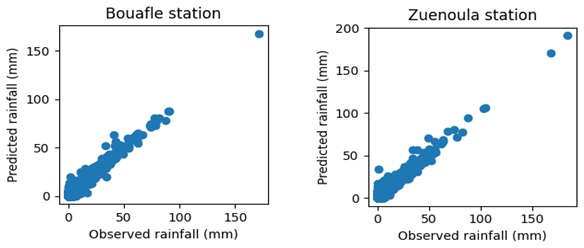
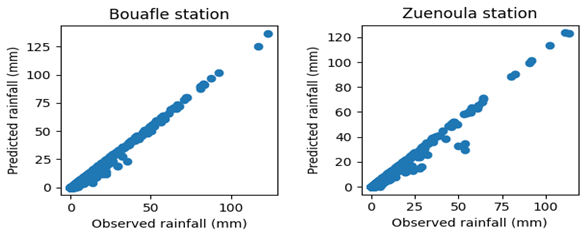
The performance results of the developed models Long Short-Term Memory (LSTM), Extra Trees (ET), Random Forest (RF), and eXtreme Gradient Boosting (XGB) during the Training and Validation phases at the respective forecasting horizons t + 1, t + 3, and t + 7 are reported in Tables 3, 4, and 5. In addition to these results, scatter plot representations for each station, calculated using the best-performing model, are provided in Figs. 9 and 10.

Table 3 Model performance at the t + 1 forecasting horizon.

Table 4 Model performance at the t + 3 forecasting horizon.

Table 5 Model performance at the t + 7 forecasting horizon.

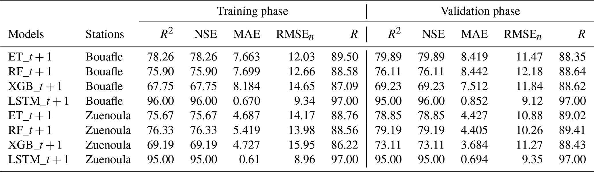
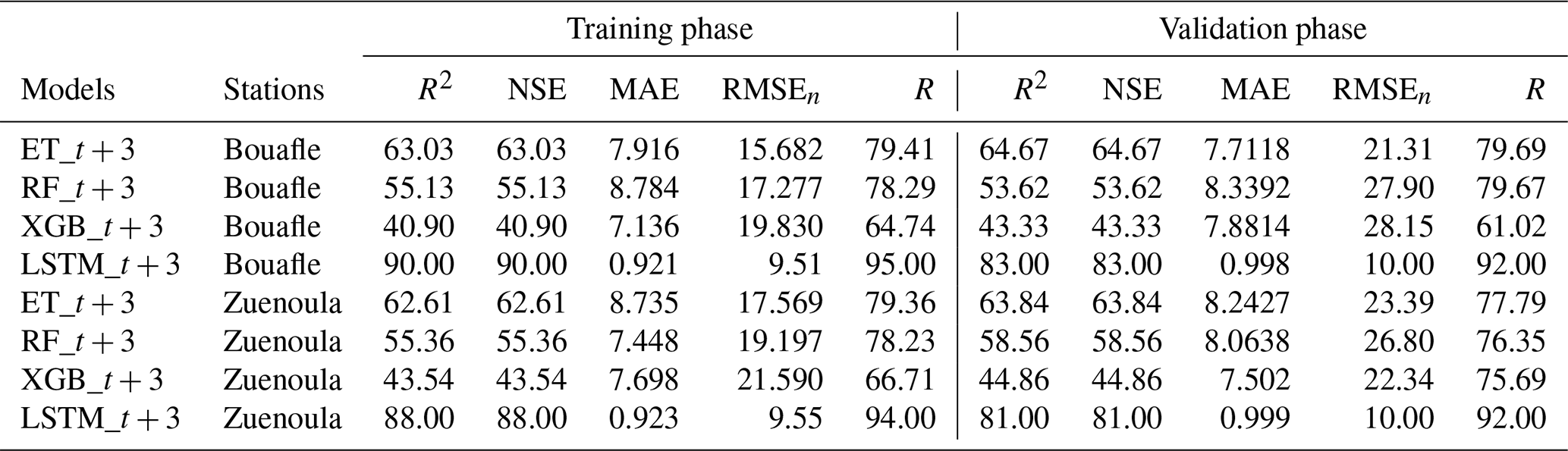
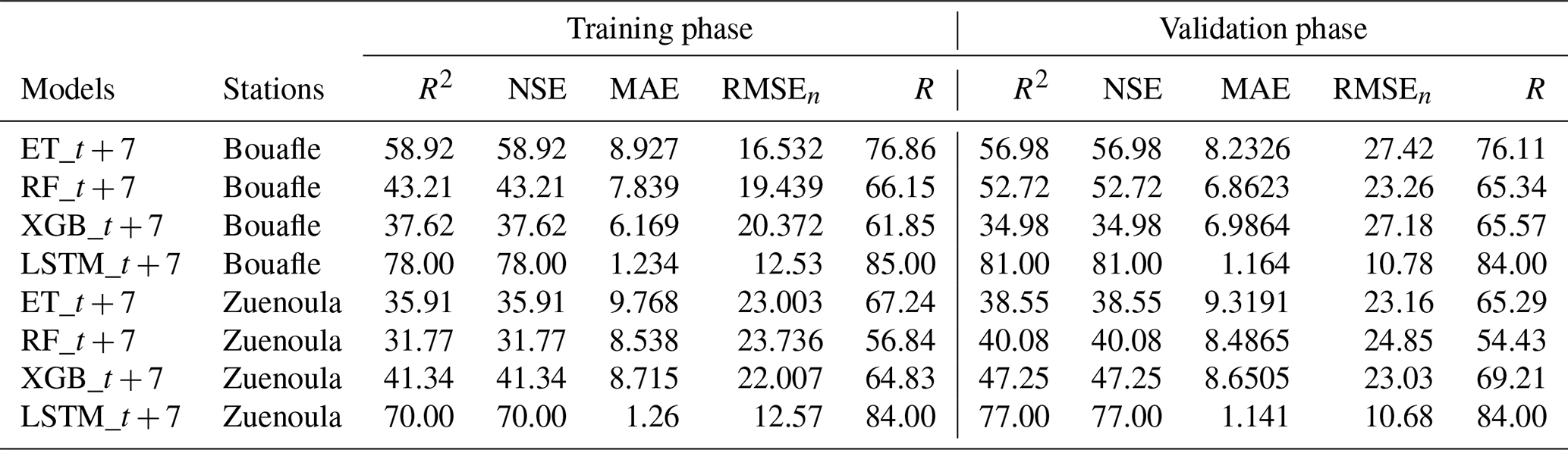
The combined analysis of the results (Tables 3, 4, and 5) highlights distinct behaviors depending on the model and the forecast horizon. At the t + 1 horizon, the LSTM model stands out as the most accurate. It exhibits the lowest RMSE, a normalized RMSE below 10 %, and an MAE under 1 mm, reflecting excellent precision. These performances are further supported by high R² and NSE values (≥ 95 %) for both stations, demonstrating the model's ability to faithfully reproduce the daily precipitation dynamics at Bouaflé and Zuénoula. At the t + 3 horizon, the LSTM maintains its high performance. The RMSE remains stable, with a normalized RMSE below 10 % and a low MAE, indicating the robustness of the model despite the extended forecast horizon. R² values range between 88 % and 90 %, confirming the consistency of the predictions and the model's capacity to capture daily variability. At the t + 7 horizon, the LSTM remains the only model providing statistically reliable forecasts. It maintains a controlled RMSE, a normalized RMSE below 10 %, and MAE values between 1.141 and 1.26 mm, while R² values remain between 70 % and 81 %. These results show that the LSTM can still provide acceptable forecasts, unlike other models (RF, ET, XGB), whose performances degrade significantly at this horizon. The RF and ET models, although effective at the t + 1 horizon with relatively low RMSE and R² and NSE values between 75 % and 80 %, see their performance gradually decrease as the horizon increases. At t + 3, their RMSE rises significantly (normalized RMSE 10 %–16 %) and MAE increases, while R² often drops below 65 %. By t + 7, their performance becomes very limited, with very high RMSE and normalized RMSE, MAE exceeding 7 mm, and NSE values sometimes below 40 %. The XGB model is the least performing across all horizons, with high RMSE, higher normalized RMSE compared to other models, and high MAE, reflecting its limited ability to capture daily precipitation variability. Its R² values range from 37 % to 70 %, confirming its inability to accurately reproduce the time series dynamics. These results are primarily explained by the LSTM's ability to model long-term temporal dependencies and the nonlinearities inherent in daily precipitation series, in contrast to ensemble models (RF, ET, XGB), whose tree-based architectures cannot efficiently capture the sequential structure of the data. Finally, the graphical representation of simulated versus observed data by the LSTM at the t + 1 horizon (Figs. 9 and 10) shows a point cloud aligned along a straight line during both training and validation. This alignment underscores the strong correlation between RMSE, MAE, and the actual observations. A few points deviate from the main trend, reflecting LSTM estimation errors and confirming the calculated normalized RMSE and MAE values.

Figure 9 Scatter plots during the training phase of the LSTM model at t + 1.

Figure 10 Scatter plots during the validation phase of the LSTM model at t + 1.

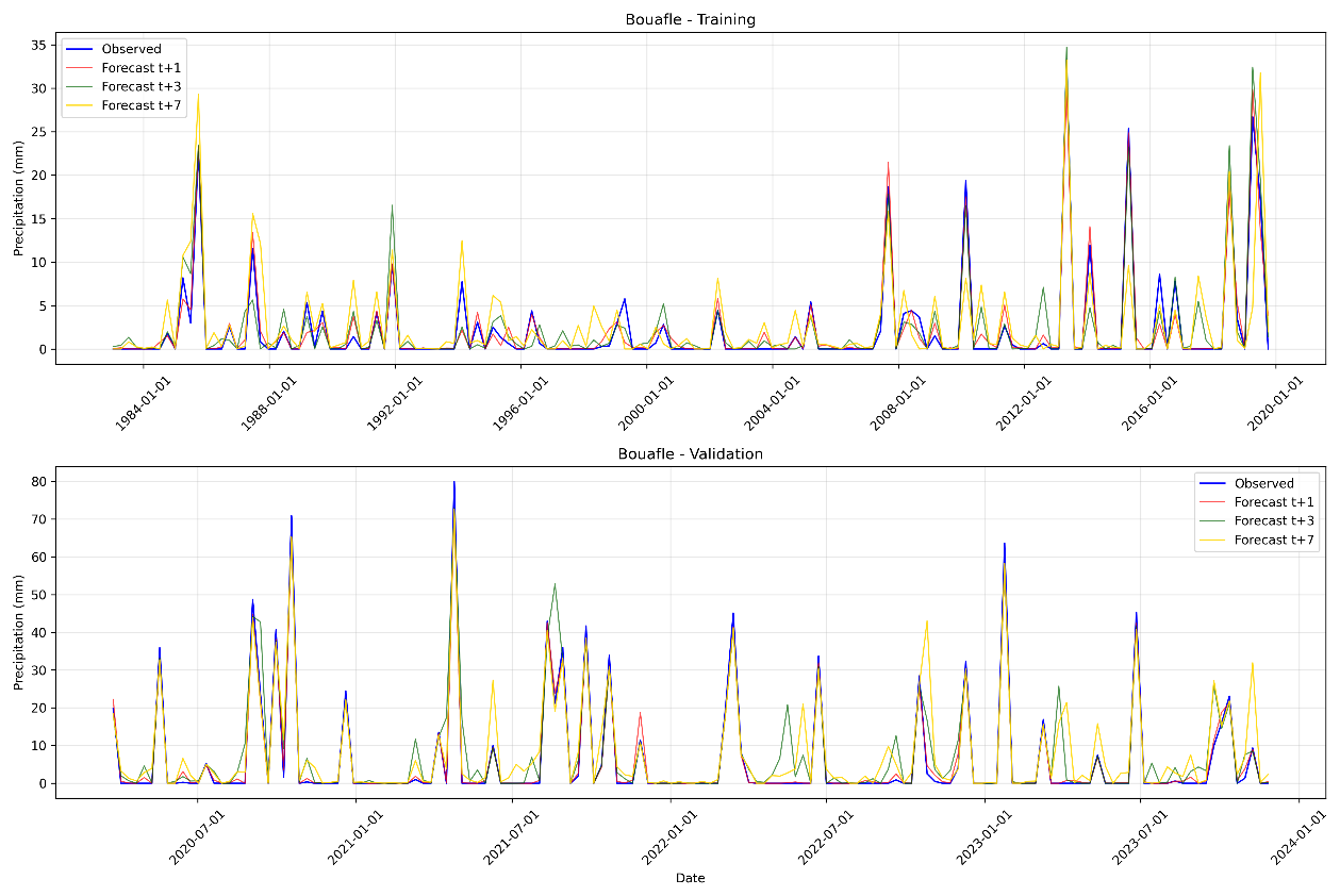
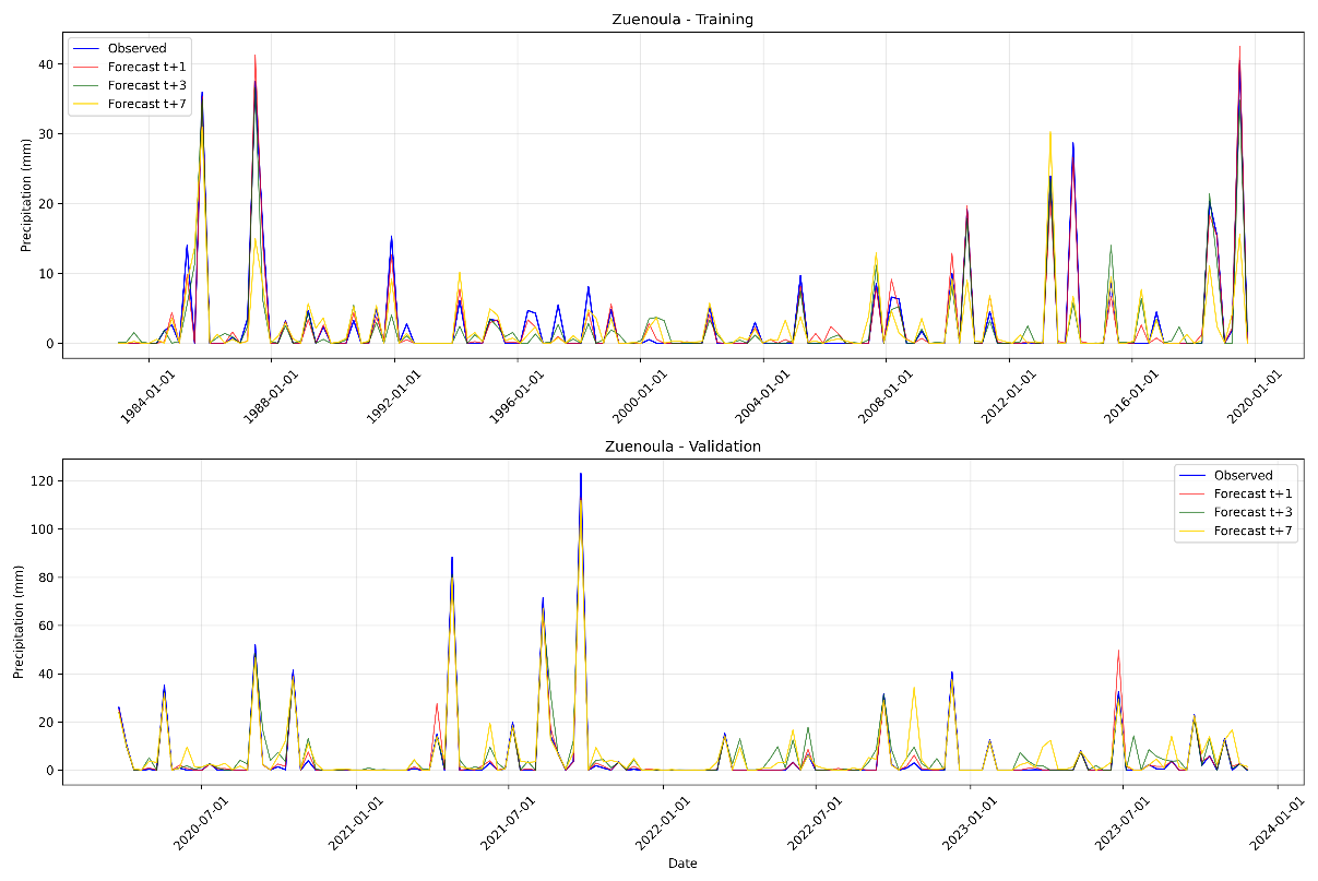
The pluviograms shown in Figs. 11 and 12 were obtained during the Training and Validation phases of the LSTM model at t + 1, t + 3, and t + 7. The analysis of the pluviograms (Figs. 11 and 12) compared to observations in Bouaflé and Zuenoula highlights a progressive deterioration in performance as the forecasting horizon increases. In Bouaflé, during the training phase, the t + 1 forecast generally reproduces the observed rainfall dynamics well, particularly the timing of peaks and dry periods, although some maxima are slightly underestimated or overestimated. At t + 3, the agreement remains satisfactory for moderate events, but a greater dispersion is observed around intense peaks, reflecting increased errors and a loss of precision in amplitude estimation. At t + 7, the discrepancies become more pronounced; although the model is still able to capture the occurrence of major rainfall events, their intensity is estimated more irregularly. During the validation phase, this trend becomes even more evident. At t + 1, the model maintains a good ability to detect extreme events, even if some high peaks show noticeable differences. At t + 3, the variability of the estimates increases, particularly for heavy rainfall events, where both underestimations and significant overestimations are observed. At t + 7, the dispersion is the most pronounced, with maximum intensities reproduced more irregularly, especially during extreme events. In Zuenoula, during training, the t + 1 forecast shows very good agreement with observations. Rainfall peaks, including intense episodes, are generally well reproduced in terms of both timing and amplitude, despite a few slight occasional overestimations. At t + 3, the overall rainfall dynamics remain well captured, but greater variability is observed around the maxima, with more noticeable discrepancies for moderate to strong events. At t + 7, the differences become more apparent, with peak intensities sometimes attenuated or, conversely, amplified, indicating a progressive loss of precision in the estimation of extremes. During validation, this trend becomes more pronounced. The t + 1 forecast retains satisfactory skill in detecting major events, including heavy rainfall, although some extreme peaks show significant amplitude differences. At t + 3, divergences become more frequent, particularly for very intense episodes, where significant underestimations or overestimations are observed. At t + 7, dispersion is the most pronounced, with uncertain reproduction of extreme maxima. Overall, in Zuenoula as in Bouaflé, the results confirm robust performance at short lead time (t + 1), still acceptable accuracy at medium lead time (t + 3), and a more marked degradation at longer lead time (t + 7), particularly for extreme rainfall events, which is consistent with the expected behavior of multi-horizon forecasting models.

Figure 11 Rainfall charts of the Bouaflé station.

Figure 12 Rainfall charts of the Zuénoula station.

5.4 Quality of the rainfall estimates

The results of the quality analysis of the rainfall estimates are presented in accordance with the methodological approach detailed in Sect. 4.5.2.

5.4.1 Residual analysis

The analysis of Table 6 indicates the following:

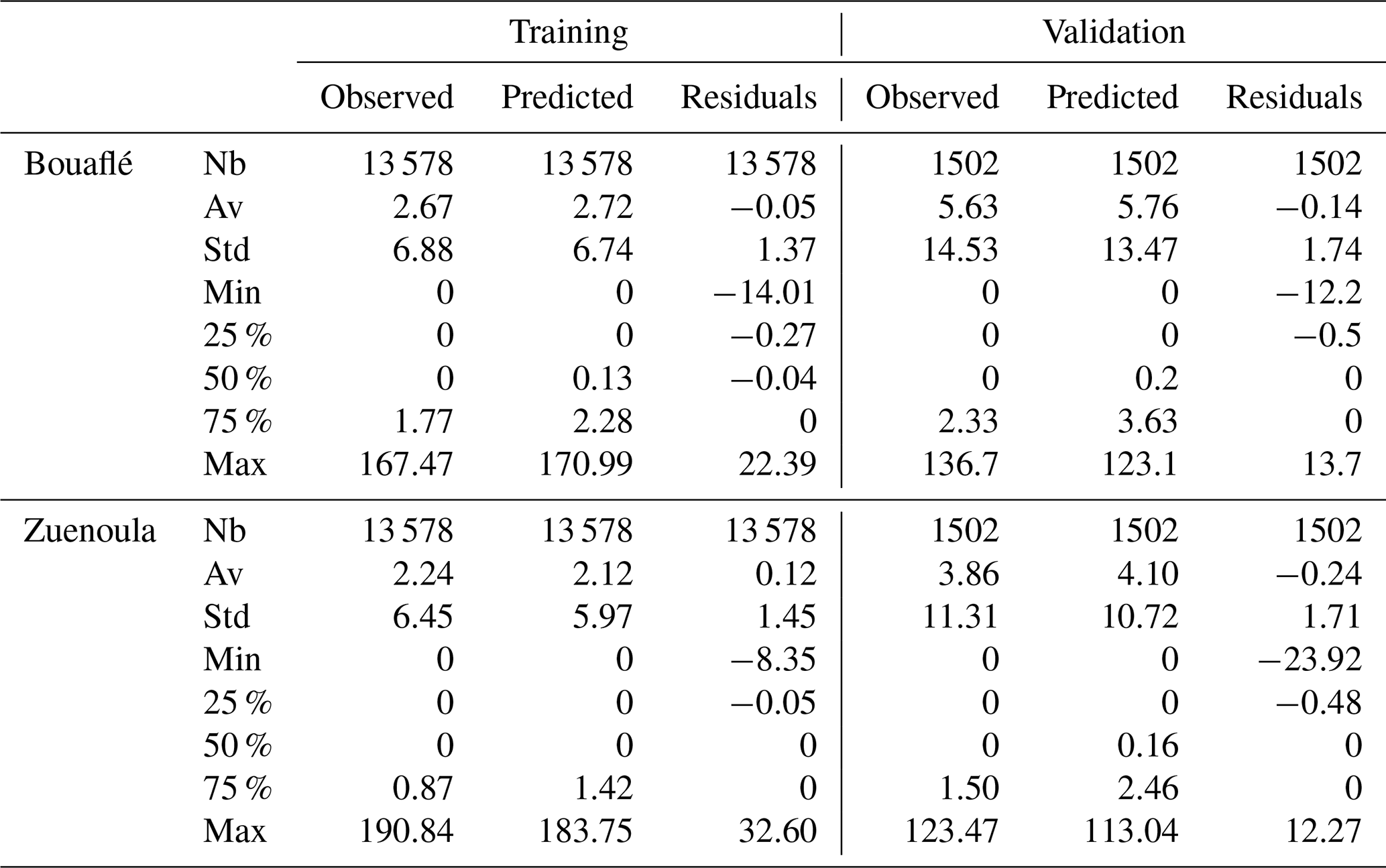
• At the Bouaflé station. During the training phase, predicted precipitation ranges from 0 to 170.99 mm, with a mean of 2.72 mm. The mean residual, representing the average difference between observed and predicted precipitation, is approximately −0.05 mm, indicating that the model reproduces the observed in situ precipitation very closely on average. During the validation phase, predicted precipitation ranges from 0 to 123.1 mm, with a mean of 5.76 mm. Residuals vary between −12.2 and 13.7 mm, demonstrating that the LSTM model at t + 1reproduces observed values accurately and captures the same temporal trends as the observed data.

• At the Zuenoula station. During training, predicted precipitation has a mean of 2.12 mm, very close to the observed mean of 2.24 mm. The minimum and maximum predicted values are 0.00 and 183.75 mm, respectively, which are comparable to the observed extremes of 0.00 and 190.84 mm. The mean residual is approximately 0.12 mm, and 75 % of predicted precipitation values have residuals below 0.00 mm. During validation, a similar trend is observed, with residuals ranging from −23.92 to 12.27 mm and a mean of −0.24 mm, reflecting minor deviations of the LSTM model at t + 1. These results indicate that the LSTM model at t + 1accurately reproduces observed precipitation during the training phase.

Table 6 Statistical parameters of predicted and observed rainfall.

5.4.2 Normality test of rainfall residuals

The results of the Kolmogorov–Smirnov tests performed on the residual rainfall values during the training and validation phases are presented in Table 7.

Table 7 Kolmogorov–Smirnov (KS) test of residuals calculated by LSTM model at t + 1.

The analysis of Table 7 indicates that during the training phase, the Kolmogorov–Smirnov (KS) test values for each station range between 0.3289 and 0.3321. All corresponding p-values are 0.0000, which is below the significance level of α= 0.05. These results suggest rejection of the null hypothesis (H₀) and acceptance of the alternative hypothesis (H₁) for both study stations, indicating that the residuals computed during the training phase do not follow a normal distribution.

During the validation phase, the KS test values for each station range from 0.3116 to 0.3269, with corresponding p-values of 0.0000, also below the significance threshold of α= 0.05. These results again indicate rejection of (H₀) and acceptance of (H₁), showing that the residuals during validation are not normally distributed.

In summary, residuals obtained from the various training and validation phases of the LSTM model at t + 1 do not follow a normal distribution. Nevertheless, analyzing the dispersion of residuals remains necessary to assess the behavior and accuracy of the model's predicted data.

5.4.3 Relationship between predicted rainfall and residuals

The analysis of Figs. 13 and 14 indicates that at the Bouaflé and Zuenoula stations, during the training phase, most residual values are clustered around zero. Furthermore, the relationship between residuals and predicted precipitation demonstrates a good fit for low precipitation values, which correspond to the majority of points concentrated near zero. In contrast, for high precipitation events, larger errors are observed, resulting in significant dispersion of points in each plot. These observations suggest that the model tends to underestimate or overestimate certain high-intensity precipitation events at both stations.

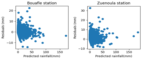
Figure 13 Distribution of residuals with respect to predicted rainfall during the Training phase.

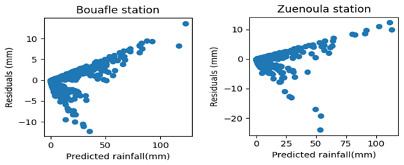
Figure 14 Distribution of residuals with respect to predicted rainfall during the Validation phase.

During the validation phase, residuals also show a strong clustering around zero; however, dispersion remains evident for higher precipitation values. This distribution reflects a continued tendency of the model to under- or overestimate some of the intense precipitation events. Overall, the LSTM model at t + 1 proves to be the most effective neural network approach for forecasting daily rainfall time series at the Bouaflé and Zuenoula stations within the study area. It reproduces, in most cases, more than 95 % of the observed precipitation at the t-step forecast. Predicted precipitation follows similar temporal patterns and variability as the observed data. Nevertheless, the model exhibits a tendency to slightly overestimate or underestimate extreme precipitation peaks.

5.4.4 Relationship between observed rainfall and residuals

A detailed analysis of the residuals (Figs. 15 and 16) reveals the presence of bias across all precipitation classes, both at Bouaflé and Zuénoula, during training and validation. A class-wise examination shows that the errors are not randomly distributed around zero. At Bouaflé, during training, low precipitation events (0–26 mm) exhibit a slight positive residual trend for some categories, indicating underestimation. In contrast, for intermediate classes (26–31 mm), residuals are predominantly negative, reflecting a tendency to overestimate moderate precipitation. This trend becomes more pronounced for high precipitation events (> 31 mm), where negative residuals dominate and the error magnitude increases significantly. Thus, the model exhibits an intensity-dependent bias: underestimation for low values and increasing overestimation as precipitation intensity rises. At Zuénoula, this behavior is even more marked during training. Several low-intensity points deviate more from zero, while residuals for intermediate classes become strongly negative. For high precipitation events, overestimation is pronounced, with large deviations. This indicates a bias that increases with precipitation intensity, suggesting poor calibration of the model for extreme events. During validation, these biases persist, confirming that they are not merely a training artifact. At Bouaflé, low precipitation events remain slightly underestimated, whereas intermediate and high classes are mostly overestimated, with greater dispersion than in training. At Zuénoula, the bias structure is similar: high precipitation events are consistently overestimated, and errors increase with intensity, highlighting the model's persistent difficulty in accurately reproducing out-of-sample extremes.

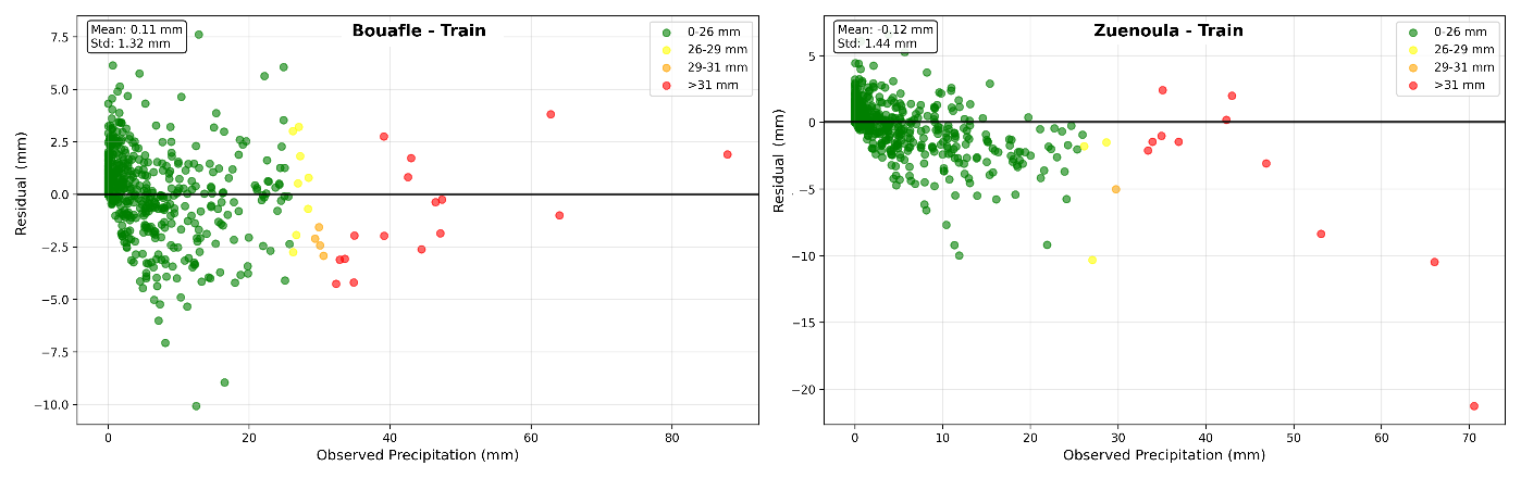
Figure 15 LSTM model residuals as a function of observed rainfall, grouped by rainfall intensity classes in training phase.

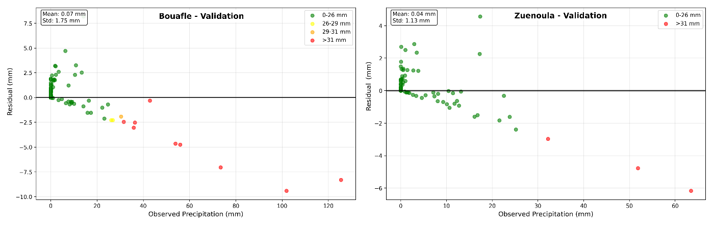
Figure 16 LSTM model residuals as a function of observed rainfall, grouped by rainfall intensity classes in validation phase.

In summary, although the overall mean of residuals may approach zero, this masks compensatory biases between classes. The model exhibits a directional error dependent on precipitation intensity, characteristic of a nonlinear calibration issue, where low, medium, and high rainfall are not reproduced with the same accuracy. Despite these limitations, the results show overall satisfactory performance for predicting low to medium precipitation, which constitutes the majority of rainfall occurrences at both stations. The consistency observed between training and validation phases reinforces the model's robustness for operational use, particularly in early warning contexts where accurate reproduction of ordinary rainfall is essential.

6 Discussion

Several models, including Random Forest (RF), Extra Trees (ET), XGBoost (XGB), and Long Short-Term Memory (LSTM), were developed to predict daily precipitation observed at the Bouaflé and Zuenoula rainfall stations. This approach required the establishment of three distinct forecasting frameworks corresponding to time steps t + 1, t + 3, and t + 7, in order to analyze model performance across longer temporal sequences. The results highlight marked differences in performance among the tested forecasting models (ET, RF, XGB, and LSTM) and a strong dependence on the forecasting horizon. Overall, the LSTM model emerges as the most robust and highest-performing approach for predicting daily precipitation at the Bouaflé and Zuenoula stations, regardless of the time horizon considered. At the short-term horizon (t + 1), the high performance of the LSTM characterized by R² and NSE values exceeding 95 % and low errors (MAE and normalized RMSE) demonstrates excellent reproduction of daily precipitation dynamics. Comparable results were reported by Hakizimana (2023) in Burundi, with determination coefficients between 0.84 and 0.98 and Nash indices ranging from 0.74 to 0.95, as well as by Endalie et al. (2022) in Ethiopia, who reported an NSE of 0.81 and a Pearson correlation coefficient of 0.9972 (99.72 %) for daily precipitation forecasts. The model's ability to faithfully reproduce observed precipitation, confirmed in this study by the strong alignment of scatter plots and the coherence of hyetographs, suggests good generalization of the network and an absence of significant overfitting, in line with observations by Gers et al. (1999) on long short-term memory networks. In comparison, ET and RF models show satisfactory performance only at this horizon, while XGB remains less accurate, indicating a lower capacity of tree-based models to capture local rainfall variability, as reported in several comparative studies in hydrology. As the forecasting horizon increases (t + 3 and t + 7), a gradual degradation of performance is observed across all models, a phenomenon commonly reported in the hydrometeorological time series literature. However, this degradation is much less pronounced for LSTM, which maintains statistically acceptable levels of accuracy up to t + 7, unlike decision-tree-based models (ET, RF, and XGB), whose performance becomes limited at medium and long-term horizons. These findings are consistent with results reported by Hao and Bai (2023), and Waqas et al. (2024). This difference can be attributed to the intrinsic capacity of LSTM to model long-term temporal dependencies and complex nonlinearities, characteristic of daily precipitation series. As shown by Hochreiter and Schmidhuber (1997) and later by Gers et al. (1999), the LSTM architecture mitigates issues of gradient explosion or vanishing, enabling efficient learning of long-range dependencies, whereas ensemble models primarily treat observations in a static manner. Residual analysis provides additional insights into forecast quality. The non-normality of residuals, as evidenced by the Kolmogorov–Smirnov test, reveals a systematic structuring of errors across precipitation classes. This non-normality primarily reflects asymmetry and non-uniform dispersion of the residuals rather than purely random behavior. Moderate to high precipitation events are predominantly associated with negative residuals, indicating a tendency of the model to overestimate these events, whereas some low-intensity events exhibit slight underestimation. This directional organization of errors highlights an intensity-dependent bias and suggests a nonlinear calibration issue, as the different precipitation classes are not reproduced with the same level of accuracy. The increasing dispersion of residuals at higher intensities underscores the persistent difficulty of the model in accurately representing extreme events, which remains a well-documented limitation of LSTM models applied to daily precipitation series (Endalie et al., 2022). This behavior, frequently observed in Deep Learning models applied to precipitation, is attributable to the rarity, irregularity, and strong skewness of intense rainfall, which limits adequate representation during training. Analysis by rainfall intensity classes confirms that the LSTM model performs particularly well for light to moderate precipitation, which constitutes the majority of occurrences in the study area. In contrast, for heavy rainfall, errors increase, reflecting a structural limitation of the model rather than mere overfitting, since this behavior is observed in both Training and Validation phases. Recent studies similarly indicate that LSTM networks perform very well for reproducing ordinary rainfall regimes but face limitations in representing extreme events. In particular, Baste et al. (2025) showed that LSTM models struggle to extrapolate extreme precipitation in a physically realistic manner, especially when observed intensities exceed the range covered by training data. Similarly, Sham et al. (2025) highlighted a marked tendency of LSTM networks to smooth high-intensity rainfall, resulting in increasing deviations between observed and predicted precipitation during extreme events. These findings confirm that, although LSTM networks are particularly effective for modeling light to moderate rainfall, their capacity to accurately reproduce extreme precipitation remains limited. To mitigate these limitations, several approaches can be considered: (i) applying post-prediction bias correction methods to adjust systematic overestimations or underestimations; (ii) enriching the training dataset with extreme precipitation events, whether historical or synthetic, to better represent rare occurrences; (iii) incorporating additional meteorological variables or exogenous covariates to better capture factors influencing extreme rainfall; (iv) exploring hybrid models combining LSTM with physical or statistical models specifically designed for extreme event modeling; and (v) optimizing the LSTM architecture by increasing the number of layers or neurons, or by employing advanced regularization techniques to reduce asymmetry and heteroscedasticity in the residuals.

7 Conclusion

Recurrent flooding in the Marahoué region, particularly in the cities of Bouaflé and Zuénoula, highlights the pressing need for reliable and operational tools to anticipate hydrological risks and enhance early warning capabilities. In response to this challenge, this study proposed a data-driven rainfall forecasting framework based on Long Short-Term Memory (LSTM) neural networks combined with satellite-derived precipitation data. Three forecasting configurations were developed to predict daily rainfall at t + 1, t + 3, and t + 7 horizons, and their performance was systematically compared with commonly used ensemble-based reference models, namely Random Forest (RF), Extra Trees (ET), and XGBoost (XGB). The results demonstrate that the LSTM model consistently outperforms the reference models across all forecasting horizons and both study stations. At the short-term horizon (t + 1), LSTM exhibits excellent predictive skill, with R² and NSE values exceeding 95 % and low error metrics (MAE and normalized RMSE), indicating an accurate reproduction of daily rainfall dynamics. At the medium-term horizon (t + 3), LSTM maintains strong performance, confirming its robustness in capturing temporal dependencies beyond immediate lead times. Although a decline in accuracy is observed at the long-term horizon (t + 7), the LSTM remains the only model achieving statistically acceptable performance, whereas tree-based models experience a pronounced degradation. The comparative analysis confirms that the superior performance of LSTM is primarily attributable to its ability to model long-term temporal dependencies and nonlinear relationships, which are intrinsic characteristics of daily precipitation processes. In contrast, ensemble tree-based models, which treat observations in a largely static manner, show limited capacity to generalize as the forecasting horizon increases. Residual analysis further indicates that LSTM predictions are largely unbiased for light to moderate rainfall events, which dominate the rainfall regime in the Marahoué basin. However, increased dispersion and systematic underestimation are observed for high-intensity precipitation, reflecting structural limitations of deep learning models when confronted with rare and highly skewed extreme events. Despite these limitations, the overall findings confirm that LSTM-based models constitute a robust and reliable foundation for rainfall forecasting and early warning systems in data-scarce and flood-prone regions such as the Marahoué basin. Their strong performance at short and medium lead times is particularly relevant for operational flood preparedness and risk mitigation. Future work should focus on improving the representation of extreme rainfall events through the integration of additional atmospheric and climatic predictors, such as Convective Available Potential Energy (CAPE), Convective Inhibition (CIN), total column water vapor, radar reflectivity, infrared brightness temperature, and regional sea surface temperatures, particularly over the Atlantic Ocean, the Gulf of Guinea, and ENSO-related regions (e.g., Niño 3.4). Furthermore, the application of advanced hyperparameter optimization techniques and hybrid modeling strategies could further enhance long-term forecast reliability and support the development of more effective early warning systems in West Africa.