A statistical approach to unveil phytoplankton adaptation to ocean fronts

Fine-scale oceanic fronts are ubiquitous and ephemeral physical features that separate contrasting water masses, creating significant heterogeneity in the physical seascape and plankton distributions. Because phytoplankton community composition (PCC) is a key driver of marine ecosystem functioning, understanding the extent to which fine-scale fronts influence PCC is a critical challenge. However, studying PCC across and within fronts is particularly difficult due to data scarcity and high biophysical variability. We developed a tailored statistical model to characterize PCC within an oceanic front we studied in the Mediterranean Sea. We modeled the frontal community as a finite mixture model with three components: two communities of adjacent water masses and a potential front-adapted community. Each component was further considered as a discrete mixture of an unknown number of multivariate Gaussian sub-components. First, we used an Expectation–Maximization algorithm to estimate the Gaussian parameters and determine the optimal number of sub-components based on in situ datasets of the PCC within a frontal zone and its adjacent water masses. Second, a hierarchical Bayesian approach was applied to estimate the weight of all components within the frontal dataset. Our analysis suggests that within the front a new community component, distinct from those in adjacent water masses, accounts for 70 % of the frontal community, indicating that a specific phytoplankton community can emerge in fine-scale oceanic fronts. Despite the limited number of frontal observations, our Bayesian modelling approach provides statistical evidence of the front's influence on phytoplankton community composition, effectively overcoming data scarcity and high variability.

1 Introduction

The oceanic seascape resembles a dynamic mosaic of contrasting water bodies, separated by boundaries known as fronts (Acha et al., 2015). Fine-scale fronts (1–100 km, day–weeks) arise from the interaction of water masses with distinct origins and characteristics (such as temperature and salinity) and are ubiquitous in the ocean (McWilliams, 2021). These fronts influence the environment from the surface to deeper ocean layers, impacting biogeochemical processes by modulating material transport; both by acting as horizontal barriers and by generating vertical fluxes (Mahadevan and Archer, 2000). In particular, upward currents can transport nutrients from deeper layers, supporting enhanced biodiversity and biomass (Lévy et al., 2015; Clayton et al., 2017).

Among the biological communities affected by fine-scale frontal dynamics, phytoplankton are especially affected due to their limited motility. Phytoplankton communities (i.e. specific assemblages of taxa) form the base of the trophic chain , produce oxygen by photosynthesis and play a key role in the biogeochemical cycling of carbon, nitrogen, and phosphorus, thereby regulating marine ecosystem functioning and contributing to global climate processes (Litchman et al., 2010; Eggers et al., 2014). Significant heterogeneity in phytoplankton communities is observed throughout the ocean, and key questions remain regarding the factors that shape their composition and the underlying drivers of their remarkable diversity (Sournia et al., 1991; Bianchi and Morri, 2000; Coll et al., 2010). One plausible hypothesis is that fronts delineate distinct habitats, thereby maintaining diversity by structuring species distributions and interactions. Given their potential impact on biological processes across the trophic chain, fine-scale fronts are a critical area of study. Moreover, fine-scale effects on biogeochemical cycles in the context of global warming are of great concern (Yang et al., 2023; Lévy et al., 2024).

The study of frontal phytoplankton communities needs dedicated cruises (Lévy et al., 2024) with high-frequency sampling to have enough data to perform robust statistical analysis. A few in situ studies suggested that fronts are either i) areas where environmental conditions allow the development of an inherent phytoplankton community (Taylor et al., 2012; Mangolte et al., 2023; Clifton Gray et al., 2024), or ii) simple boundaries between two contrasting water masses and their associated phytoplankton communities (Clayton et al., 2014; Mousing et al., 2016; Marrec et al., 2018; Tzortzis et al., 2021). However, these suggestions are hindered by significant challenges of obtaining in situ measurements within fine-scale fronts as they are small, short-lived, and difficult to track, leading to a lack of observations (Lévy et al., 2012). In addition, phytoplankton organisms respond rapidly to their environment (Collins et al., 2014), with large variations in abundance and biomass, which in turn result in highly variable datasets (i.e. non-Gaussian, skewed or multimodal distributions).

Consequently, a first key step lies in applying statistical analyses to scarce variable observations. When priors (i.e. assumed distribution before incorporating any data or observations) are properly defined, Bayesian statistics are known for their ability to capture signals even with scarce and highly variable data, providing reliable statistical inference even with small sample sizes (McNeish, 2016). A second key step in studying the phytoplankton community composition (hereafter “PCC”) in different areas, such as fronts and their adjacent water masses, is to manage the complexity of multidimensional datasets characterized here by different phytoplankton types. Gaussian mixture modelling (hereafter “GMM”) is used to model multiple signals that are assumed to follow normal distributions (McLachlan and Peel, 2000). By modelling multiple Gaussian components, GMM can model complex (i.e., non-Gaussian) distributions (Birgé, 1983). Originally introduced by Pearson (1894) to model heterogeneous biological data, GMM has since been widely applied in oceanography, for example to analyse krill cohort dynamics (Shaw et al., 2021) and phytoplankton classification (Hyrkas et al., 2016). Phytoplankton communities consist of different groups (e.g., cyanobacteria, picophytoplankton constituted by cells between 0.2 and 2–3 µm in size, nanophytoplankton constituted by cells between 2–3 and 20 µm in size, etc.). Applying GMM to a multivariate dataset would help quantify the ecological signals of different phytoplankton communities (i.e., bloom of a specific group, a response to a nutrient pulse), especially when dealing with complex, overlapping distribution of groups. This is useful when the assumptions of traditional statistical tests are not met in the case of a mixture (e.g. normality and homoscedasticity).

Our study focuses on the Mediterranean Sea due to its combination of moderately energetic physical processes and oligotrophic conditions, which resemble those in the global ocean (Bethoux et al., 1999). We build on the previous study by Tzortzis et al. (2021) conducted south of Balearic islands where a front separating Atlantic waters recently entering the Mediterranean from saltier surface waters of the western Mediterranean was observed. That study demonstrated that this front plays a significant role in the structuring of PCC by segregating different classes of phytoplankton sizes between the two adjacent water masses, resulting in two distinct communities. However, a potential front-adapted phytoplankton community could not be identified due to in situ sampling limitations leading to a small number of observations in the front.

In this article we developed a statistical approach combining GMM and Bayesian methods that allowed us to estimate the presence of communities using the phytoplankton biomass data within the well-defined physical frontal region previously studied by Tzortzis et al. (2021). This provides a novel methodological framework for investigating the complex interactions between fine-scale physical and biological seascapes, while accounting for the challenges of obtaining data at such scales. We ask the following questions: What is the structure of the community that might be formed at the front? Is there a frontal community as a mixture, where the expected community results from the combination of the adjacent water communities, or is there another community resulting from the intrinsic frontal characteristics? Answering these questions would provide valuable insights into the role of fine-scale oceanic fronts in the distribution of marine biodiversity. This is particularly important in frontal areas where observations are rare.

This article is structured as follows: In Sect. 2, we describe the data, followed by the modelling approach in Sect. 3. In Sect. 4, we present the results, which are discussed in Sect. 5. Finally, we conclude the study in Sect. 6.

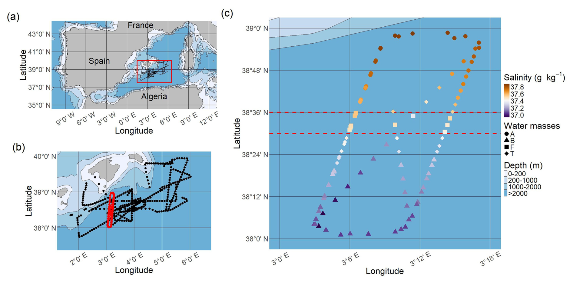
Figure 1 Study area and sampling strategy. (a) Map of the north-western Mediterranean Sea; the red rectangle corresponds to the PROTEVSMED-SWOT study area. (b) Map of the sampling area; the black dots correspond to cytometric samples collected throughout the entire cruise (outside dataset) and the red dots to samples from the NS-Hippodrome. (c) Absolute salinity distribution (g kg⁻¹) along the NS-Hippodrome. The shape of the dots depends on the water masses they belong to. The dashed red lines correspond to the latitudinal limits of the front. Note that to highlight the sampling points, no geographic projection is used in this panel. Maps were produced using Natural Earth open access data.

2 Study area and data collection

2.1 Cruise strategy and hydrology

During the PROTEVSMED-SWOT campaign (May 2018, south of the Balearic Islands, Dumas, 2018), we implemented a sampling strategy to cross a frontal zone separating two distinct water masses several times, with a North-South, “hippodrome” shaped route (hereinafter NS-Hippodrome, Fig. 1) (Tzortzis et al., 2021). High-resolution physical and biological surface measurements were collected using a CTD sensor mounted on a towed vehicle, a thermosalinograph (TSG) and an automated flow cytometer installed on the surface water intake of the TSG circuit. By employing an adaptive Lagrangian sampling strategy, we tracked physical and biological structures in both space and time, identifying a fine-scale frontal zone separating the two water masses A and B, each characterized by contrasting abundances of nine phytoplankton groups defined by flow cytometry (Tzortzis et al., 2021). To capture the phytoplankton diel cycle, both water masses were continuously sampled along the NS-Hippodrome from 11 to 13 May, 2018. This approach allowed us to capture the diel cycle in both A and B similarly, reducing biases from cell size and division. As a result, any differences in cell abundance between the A and B water masses are not related to diel cycle variations, making the observations independent and identically distributed (hereafter i.i.d.).

Based on extensive analysis of temperature and salinity in the water column and across the zone, Tzortzis et al. (2021) characterized the frontal area around 38.32° N. They stated that surface salinity was a good marker for the water masses in the visited area (Fig. 1c). The salinity gradient during the cruise (see Fig. A1) indicates that water mass A is characterized by a salinity ≥ 37.6 g kg⁻¹, and water mass B by a salinity ≤ 37.3 g kg⁻¹. The front F lies between these two isohalines. The frontal zone definition also followed a geographic criteria, 38.36° N ≥ Latitude ≥ 38.30° N, corresponding to the measurement locations (Tzortzis et al., 2021). To focus on the frontal zone, measurement points that lay within the salinity range of the front but outside of its geographical boundaries were considered as part of a transitional zone (T) and were not used for the data analysis. In total, 30 samples were collected in A, 44 in B, 11 in F and 17 in T.

2.2 Flow cytometry

Automated flow cytometry enables high-frequency seawater sampling and analysis to identify phytoplankton groups based on their optical scattering and fluorescence properties (Dubelaar et al., 1989; Thyssen et al., 2009, 2015). The CytoSense flow cytometer (Cytobuoy b.v., Netherlands) uses a sheath fluid of 0.1 µm filtered seawater to align and guide individual particles (cells) through a 488 nm laser beam. As cells interact with the laser beam, multiple optical signals are simultaneously recorded for each particle (cell).

First, forward scatter (FWS) and sideward scatter (SWS) are measured, providing insights into particle size, shape, and granularity. Second, fluorescence signals from photosynthetic pigments are also detected using photomultiplier tubes: red fluorescence (FLR) from chlorophyll and orange (FLO) fluorescence from phycoerythrin. Sequential protocols are run sequentially every 30 min, to analyse samples by phytoplankton size class. The first protocol (FLR6) had a FLR trigger threshold fixed at 6 mV and could analyze a volume of 1.5 cm³. It was dedicated to the analysis of the picophytoplankton (< 2 µm). The second protocol (FLR25) targeted nanophytoplankton and microphytoplankton (> 2 µm) with a FLR trigger level set at 25 mV and an analysed volume of 4 cm³.

Data acquisition was performed using CytoUSB software (Cytobuoy) and analyzed with CytoClus (Cytobuoy). The cytometer produces 2D cytograms, graphical representations that plot individual particles according to their optical signals, highlighting distinct populations based on scattering and fluorescence properties. Within these dot clouds, we manually identified clusters that serve as proxies for functional phytoplankton group (Peeters et al., 1989; Thyssen et al., 2008). CytoClus provides cell abundances (cells cm⁻³) and mean optical signal intensities for each phytoplankton group.

Nine phytoplankton groups were identified (Tzortzis et al., 2021): one cyanobacterial group, Synechococcus (Syne, 1,µm); four picoeukaryote groups (Pico1, Pico2, Pico3, PicoHFLR, 0.2–2 µm); two nanoplankton groups (SNano, RNano, 2–20 µm), cryptophytes (Crypto, 10–50 µm); and one microphytoplankton group (Micro, 20–200 µm). Abundances (number of cells) are converted into carbon biomass (mmolC m⁻³) using allometric relationships described in Tzortzis et al. (2023) and Oms et al. (2024). Importantly, there are huge size, biomass and abundance contrasts between the nine phytoplankton groups (Figs. A2 and A3).

3 Methods

3.1 Model formulation

We denote by Com the random vector characterizing a community. It is composed of the biomass of the 9 phytoplankton groups described previously. We assume that the biomass distribution of the community in the front, denoted by Com^F, is mathematically described as a finite discrete mixture of three random components corresponding, respectively, to the communities of water masses A (Com^A) and B (Com^B) and an unknown community (Com^C), as follows:

$$\begin{array}{}\text{(1)}& {\mathrm{Com}}^F={\mathbb{I}}_{U=A}{\mathrm{Com}}^A+{\mathbb{I}}_{U=B}{\mathrm{Com}}^B+{\mathbb{I}}_{U=C}{\mathrm{Com}}^C,\end{array}$$

where, for any generic condition 𝒯, the indicator function is defined as:

$$\begin{array}{}\text{(2)}& {\mathbb{I}}_{\mathcal{T}}=\left\{\begin{array}{ll}\mathrm{1}& \text{if condition }\mathcal{T}\text{ is satisfied},\\ \mathrm{0}& \text{otherwise}\end{array}\right.\end{array}$$

Here, U is an unobserved categorical random variable taking values in the set $\mathit{\{}A,B,C\mathit{\}}$, with the following probabilities:

$$\begin{array}{}\text{(3)}& \begin{array}{rl}P(U=A)=& {\mathit{\lambda }}_A,P(U=B)={\mathit{\lambda }}_B,P(U=C)={\mathit{\lambda }}_C,\\ & \text{ with }{\mathit{\lambda }}_A+{\mathit{\lambda }}_B+{\mathit{\lambda }}_C=\mathrm{1}.\end{array}\end{array}$$

Each observation is thus assumed to originate from one of the three communities A, B, or C, with respective weights λ_A, λ_B, and λ_C. The case where λ_C is significantly different from 0 indicates the presence of the new community C, while λ_C→0 corresponds to a mixture involving only communities A and B.

The collected observations (i.i.d., cf. Sect. 2.1) of Com^F is a table of dimension n × m, where n=11 biomass measurements and m=9 phytoplankton groups.

Multivariate normal distribution of A, B, F and T were assessed with the Henze–Zirkler's test (Korkmaz et al., 2014). Except for A, the empirical biomass distribution in B, F and T revealed non-Gaussian shapes associated with high variability for each phytoplankton group (see Fig. A2), suggesting underlying mixture structures of Gaussian distributions. Given this, we proposed that Com^A, Com^B and Com^C, are themselves issued from a mixture of, respectively, j, k and l multivariate Gaussian components, which model potential sub-communities within A, B and C as follows:

$$\begin{array}{}\text{(4)}& {\displaystyle }{\mathrm{Com}}^A& {\displaystyle }\sim \sum _{r=\mathrm{1}}^j{\mathit{\alpha }}_{Ar}\cdot \mathcal{N}({\mathit{\mu }}_{Ar},{\mathrm{\Sigma }}_{Ar}),\text{(5)}& {\displaystyle }{\mathrm{Com}}^B& {\displaystyle }\sim \sum _{s=\mathrm{1}}^k{\mathit{\alpha }}_{Bs}\cdot \mathcal{N}({\mathit{\mu }}_{Bs},{\mathrm{\Sigma }}_{Bs}),\text{(6)}& {\displaystyle }{\mathrm{Com}}^C& {\displaystyle }\sim \sum _{t=\mathrm{1}}^l{\mathit{\alpha }}_{Ct}\cdot \mathcal{N}({\mathit{\mu }}_{Ct},{\mathrm{\Sigma }}_{Ct}),\end{array}$$

where α denote the mixture weights (summing to 1 in each case), and μ∈ℝ^m, $\mathrm{\Sigma }\in {\mathbb{R}}^{m\times m}$ are the mean vectors and covariance matrices of the respective multivariate Gaussian components.

To estimate parameters μ, Σ, α and λ, and the number of components j, k and l in Com^A, Com^B and Com^C, respectively, we combined two estimation strategies: (i) an Expectation–Maximization (EM) algorithm ; and (ii) a two step Bayesian approach.

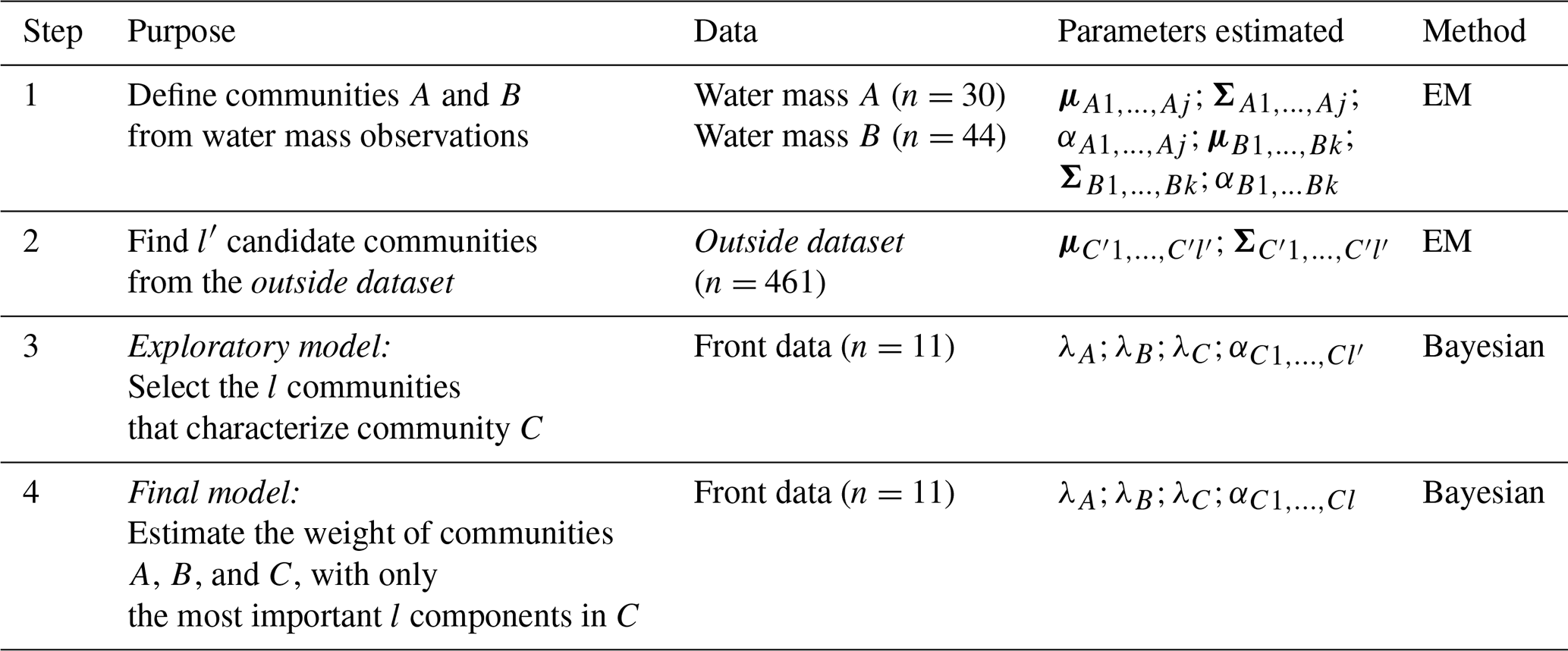
Table 1 Summary of data analysis workflow. Note that Com${}^{C^{\prime }}$ refers to the community inferred from the outside dataset, while Com^C denotes the latent community in the frontal zone. By construction, Com^C ⊂ Com${}^{C^{\prime }}$.

3.2 Estimation of Gaussian parameters using the Expectation–Maximization algorithm

Communities A and B were, respectively estimated using in situ samples using large dataset from water mass A and water mass B (step 1 in Table 1). We considered varying numbers of components $j,k\in \mathit{\{}\mathrm{1},\mathrm{\dots },\mathrm{10}\mathit{\}}$.

The potential community C cannot be directly observed in the front (due to the limited number of observations). Thus, we estimated the Gaussian parameters of likely communities to be in C from the larger dataset of the rest of the cruise, hereafter the outside dataset, which consists of 461 observations (black dots on Fig. 1b). The limitations of this approach are discussed in more detail in the Discussion section. We assumed that the community in the outside dataset denoted by Com${}^{C^{\prime }}$ is a mixture of sub-communities, large enough to represent the latent community Com^C. In other terms, we considered Com^C to be a subset of Com${}^{C^{\prime }}$. Here, we considered varying numbers of components $l^{\prime }\in \mathit{\{}\mathrm{1},\mathrm{\dots },\mathrm{20}\mathit{\}}$ to be able to propose several candidates for C (step 2 in Table 1).

For all combinations $j,k\in \mathit{\{}\mathrm{1},\mathrm{\dots },\mathrm{10}\mathit{\}}$ and $l^{\prime }\in \mathit{\{}\mathrm{1},\mathrm{\dots },\mathrm{20}\mathit{\}}$, the EM algorithm explored 14 models, each corresponding to a different structure of the covariance matrix Σ, ranging from diagonal to fully parameterized. Diagonal matrices imply no interaction between phytoplankton groups, while off-diagonal terms capture inter-group correlations.

Model selection was guided by the Integrated Completed Likelihood (ICL) criterion (McLachlan and Rathnayake, 2014), which penalizes model complexity and cluster overlap. First, optimal values of j, k and l^′ were chosen by averaging ICL values across covariance structures. Then, the best covariance model was selected for parameter estimation. In addition to μ and Σ values, the EM algorithm estimated the α weights for Com^A and Com^B. Note that for Com${}^{C^{\prime }}$, only the ${\mathit{\mu }}_{C^{\prime }}$ and ${\mathrm{\Sigma }}_{C^{\prime }}$ values were used. The weights of the candidates for Com^C, α_C, will be further estimated by the Bayesian model (see step 3 and 4 in Table 1). The R package mclust (Scrucca et al., 2023) was used to estimate the Gaussian parameters.

3.3 Estimation of components weights with Hierarchical Bayesian sampling based on scarce frontal dataset

Since very few observations were collected in the frontal region (n=11), a Bayesian approach was used to estimate the weights of components λ_A, λ_B, λ_C, see Eq. (3), and the sub components weights α_C1,…, α_Cl, see Eq. (6). Dirichlet distributions, which represent a distribution over probability distributions often used to model multivariate proportions, were used here to represent the component weights. These distributions were parameterized by a vector of positive real numbers and we proposed a non-informative prior, as follow:

$$\begin{array}{}\text{(7)}& {\displaystyle }& {\displaystyle }{\mathit{\lambda }}_A,{\mathit{\lambda }}_B,{\mathit{\lambda }}_C\sim \mathcal{D}\text{irichlet}(\mathrm{1},\mathrm{1},\mathrm{1})\text{(8)}& {\displaystyle }& {\displaystyle }{\mathit{\alpha }}_{C\mathrm{1}},\mathrm{\dots },{\mathit{\alpha }}_{Cl}\sim \mathcal{D}\text{irichlet}(\mathrm{1},\mathrm{\dots },\mathrm{1}),\end{array}$$

assigning the same weight to all coefficients. The Hierarchical Bayesian Model is decomposed in two steps. In the exploratory model (Step 3, Table 1), the l^′ candidate components identified in Com${}^{C^{\prime }}$ via EM were used to estimate their associated weights ${\mathit{\alpha }}_{C\mathrm{1}},\mathrm{\dots },{\mathit{\alpha }}_{C{l}^{\prime }}$ in Eq. (6). This step allowed to select only the most significant components among them, i.e. the l components with the highest posterior α_C values, to define Com^C. In the final model (Step 4, Table 1), we estimated the weights of the components λ_A, λ_B, λ_C, see Eq. (3), and the sub-components weights ${\mathit{\alpha }}_{C\mathrm{1}},\mathrm{\dots },{\mathit{\alpha }}_{Cl}$, see Eq. (6), with the selected l components in C.

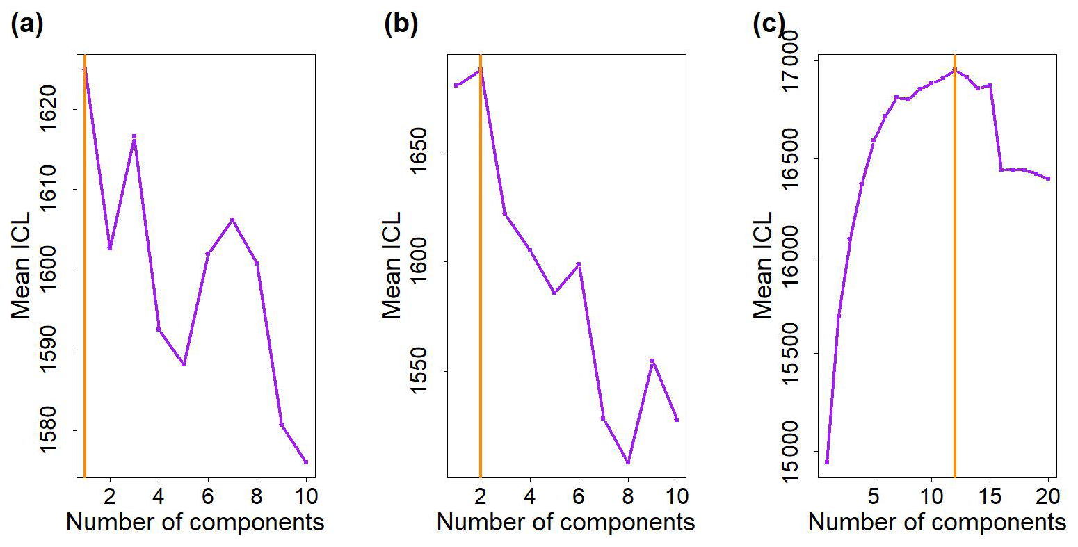
Figure 2 Values of the mean Integrated Complete-data Likelihood (ICL) in function of the number of multivariate Gaussian components. (a) Water mass A (to model Com^A). (b) Water mass B (to model Com^B). (c) Outside dataset (to propose likely parameters to model Com^C). The vertical orange lines correspond to the number of multivariate Gaussian components that reach the highest ICL values.

A sensitivity analysis was performed to test the robustness of the Bayesian inference. In particular, the sensitivity analysis aimed at assessing the robustness of the model according to the number of observations in the front, and the robustness of the model to false positive detection (i.e. detecting a new community when no communities are present in the data). For this, numerical sampling of “known” frontal community were done in two cases. First, we considered the case where front observations are only a mixture of Com^A and Com^B (i.e. simulations do not include the component Com^C, λ_C=0). Five scenarios were assessed : (1) ${\mathit{\lambda }}_A={\mathit{\lambda }}_B=\mathrm{0.5}$; (2) λ_A=0.4 and λ_B=0.6; (3) λ_A=0.6 and λ_B=0.4; (4) λ_A=0.7 and λ_B=0.3; (5) λ_A=0.3 and λ_B=0.7. Second, we considered the case where a new community exists, i.e. simulations include the component Com^C, λ_C≠0. Here the λ values used are the same as observed in the in situ dataset (see the results Sect. 4.2), and with proportion λ_A=0.45 , λ_B=0.2 and λ_C=0.35. In all cases, 5, 10, 20, 30 and 50 frontal observations were simulated 10 times. Then the Bayesian model was computed to estimate the λ values of the known communities from the simulated datasets. In addition a comparison test for equal distribution between transitional waters T and front F was performed (Székely and Rizzo, 2004).

The posterior probability distribution sampling was computed with STAN's (Carpenter et al., 2017) Hamiltonian Monte Carlo (HMC) algorithm. For all the models (i.e. exploratory and final models and sensitivity analysis) we performed four chains of 11 000 iterations to study the convergence. The first 10 000 draws of each chain were discarded (i.e. burn-in) to avoid initial sample bias. Thus, the last 1000 iterations of the four chains were used for analysis of the posterior probability distribution. Convergence was assessed with $\widehat{R}$ statistic and effective sample size. The models were computed in R (R Core Team, 2021) by means of the rstan package as interface with STAN (Stan Development Team, 2020).

4 Results

4.1 Selection of the number of components to describe phytoplankton communities

According to the mean ICL criterion, one component, A1, is enough to model Com^A (Fig. 2a), while two components (hereafter B1 and B2) are necessary to model Com^B (Fig. 2b). The weights of B1 and B2 are, respectively α_B1=0.47 and α_B2=0.53. In the outside dataset, 12 candidates components were selected (Fig. 2c).

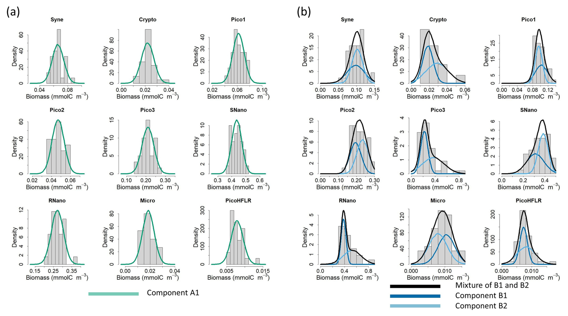
Figure 3 Fit of the multivariate Gaussian component with the observed biomass for each phytoplankton group in (a) water mass A and (b) water mass B. Histograms show the observed phytoplankton biomass distributions, and lines correspond to the density curves of the multivariate Gaussian components estimated by EM. Note that in (b) two components are necessary to model Com^B; the components B1 and B2 are weighted by their α values and the black line corresponds to the finite mixture (i.e. here the sum) of these two components.

Figure 3 shows that the estimated parameters of the multivariate Gaussian fitted well to the observed phytoplankton biomass in water mass A (Fig. 3a) and water mass B (Fig. 3b). The mixture of two components in Com^B allows to model complex biomass distributions, for e.g. skewed distribution for Crypto, Pico1, Pico3, SNano, RNano or PicoHFLR, compared with Com^A.

4.2 Modelling of the frontal phytoplankton community

The exploratory model was performed with 12 candidates components, denoted C^′ as they were estimated from the outside dataset community, to describe Com^C (see step 2 in Table 1). Using the proposed candidates, the exploratory model (whose trajectories and values of $\widehat{R}$ and effective sample size are consistent with those of a converged chain, see Fig. A4 and Table A1) was used to estimate the weights α_C and λ_A,λ_B and λ_C in the mixture (Fig. 4a and b). Among the three communities, Com^C has a higher weight (λ) in the mixture (0.787, quantile 2.5 % = 0.123, quantile 97.5 % = 0.902), followed by Com^A (0.203, quantile 2.5 % = 0.051, quantile 975 % = 0.459) and Com^B (0.065, quantile 2.5 % = 0.002, quantile 97.5 % = 0.127) (Fig. 4a and Table A1). Among the 12 candidates components in Com^C (Fig. 4b), components C^′8 and C^′10 present the highest weight, α, approx. 0.2, and to a lesser extent C^′5 and C^′6 with weights reaching 0.1. The weights of the other 8 components are below 0.05 (see Table A1 for quantiles values of the posterior distribution for each components). For the final model, performed with the most significant components, only C^′8 and C^′10 were used in Com^C as they display the highest weight. We considered C^′8 and C^′10, the most significant components in the exploratory model, as the two components of the community C, Com^C, which we call hereafter C1 and C2, respectively. The number of components in Com^C was chosen to be the most parsimonious possible. For the sake of simplicity, the components C^′5 and C^′6 were not used in the final model as they did not show strong differences relative to using only C^′8 and C^′10 in Com^C.

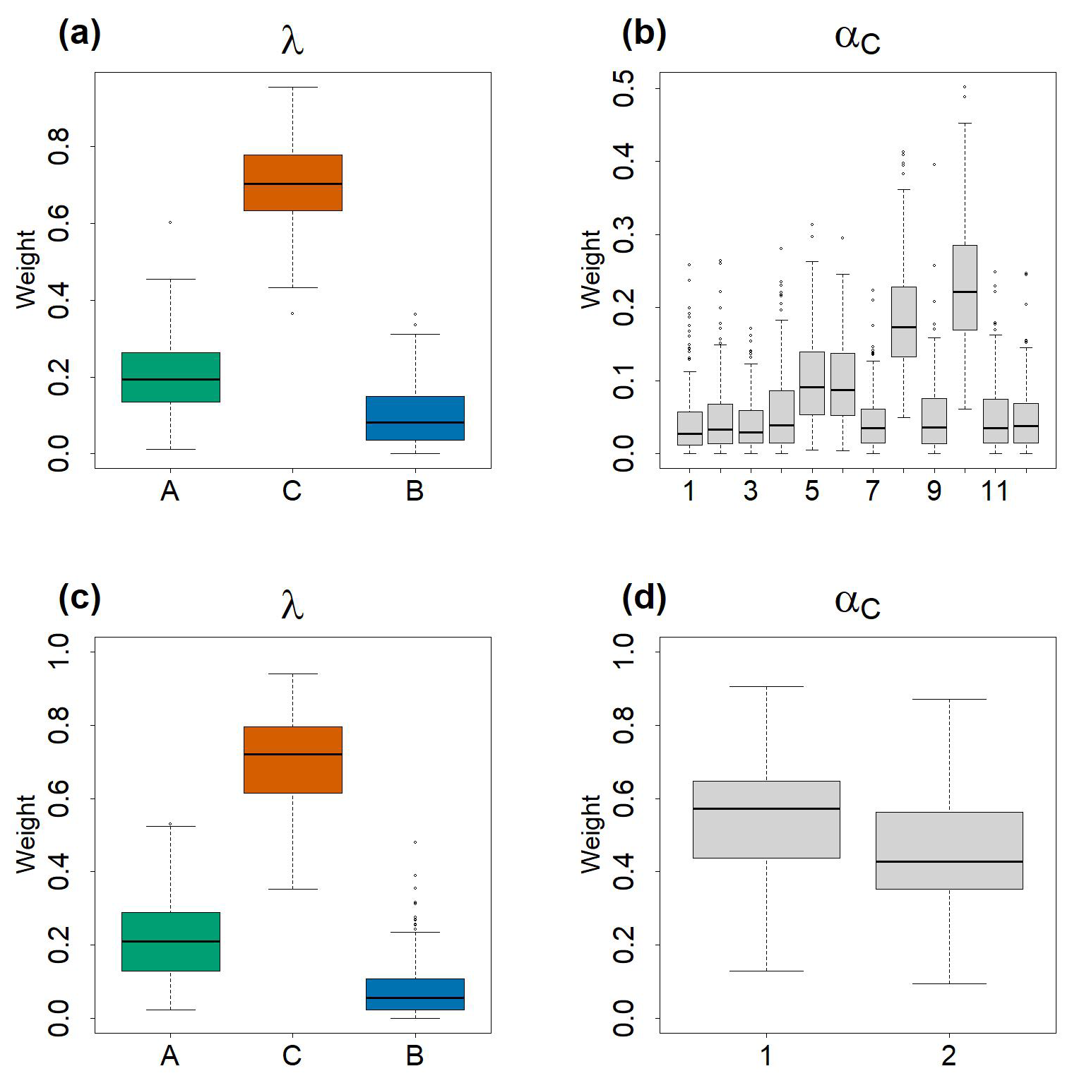
Figure 4 Boxplots of the estimated values of α_C and λ values by the Bayesian models. In total 100 values were used to construct the boxplots. Each 40 values among the 4000 iterations of the posterior distributions, generated by the HMC chains, were taken in order to avoid autocorrelation within the chains. (a) and (b) represent, respectively λ_A,λ_B and λ_C and ${\mathit{\alpha }}_{C\mathrm{1},\mathrm{\dots },C\mathrm{12}}$ of exploratory model. (c) and (d) represent, respectively λ_A,λ_B and λ_C and α_C1,C2 of the final model.

In the final model (that converged, see Fig. A5 for the trajectories, and Table A2 for convergence metrics), the estimations of λ_A,λ_B and λ_C did not vary drastically – 0.203 (quantile 2.5 % = 0.057, quantile 97.5 % = 0.467) for Com^A, 0.06 (quantile 2.5 % = 0.003, quantile 97.5 % = 0.281) for Com^B and 0.714 (quantile 2.5 % = 0.439, quantile 97.5 % = 0.901) for Com^C, Fig. 4c – relative to those observed before in the model with 12 components. In this second model, the weights of C1 (α_C1=0.55, quantile 2.5 % = 0.258, quantile 97.5 % = 0.823) and C2 (α_C2=0.45, quantile 2.5 % = 0.177, quantile 97.5 % = 0.742) were almost equivalent in the mixture (Fig. 4d and Table A2).

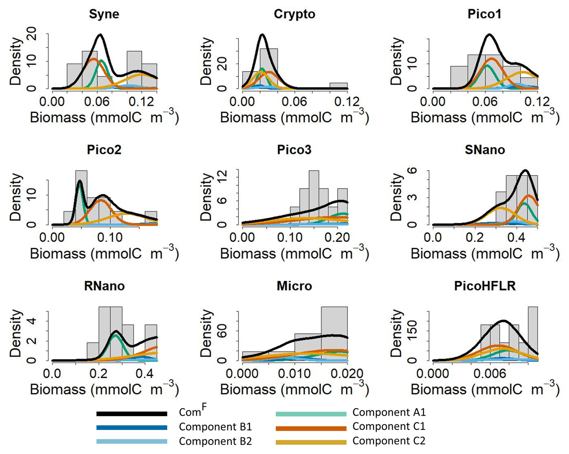
Figure 5 Fit of the multivariate Gaussian component with the observed biomass for each phytoplankton group in the front F. The histograms show the observed phytoplankton biomass distributions in the front, and the lines correspond to the density curves of the multivariate Gaussian components estimated by EM and by the Bayesian model. Note that five components are necessary to model community Com^F; all components are weighted by their λ and α values. The black line correspond to the estimated Com^F from the finite mixture (i.e. here the sum) of these five components.

Figure 5 shows how the final model fits the observed data in the front. As expected when looking at the weight λ_B (0.06, see in Fig. 4c), components B1 (dark blue curve) and B2 (light blue curve) contribute little to the global mixture (black lines), which is mostly driven by components A1 (light green curve), C1 (dark orange curve), and C2 (orange curve). Overall, the mixture of these five components captures the phytoplankton groups biomass distribution well. In some cases, the biomass distribution is bimodal (for Syne, Pico2, RNano) or skewed (for Pico1, Micro). For Pico3 and RNano a difference remained between the estimated density and the observed biomass in the front (Fig. 5). For Pico3, the μ values for C1 and C2 are the lowest (see Table 2). However due to high variance in Σ matrices the mode around 0.14–0.16 is not captured by the model.

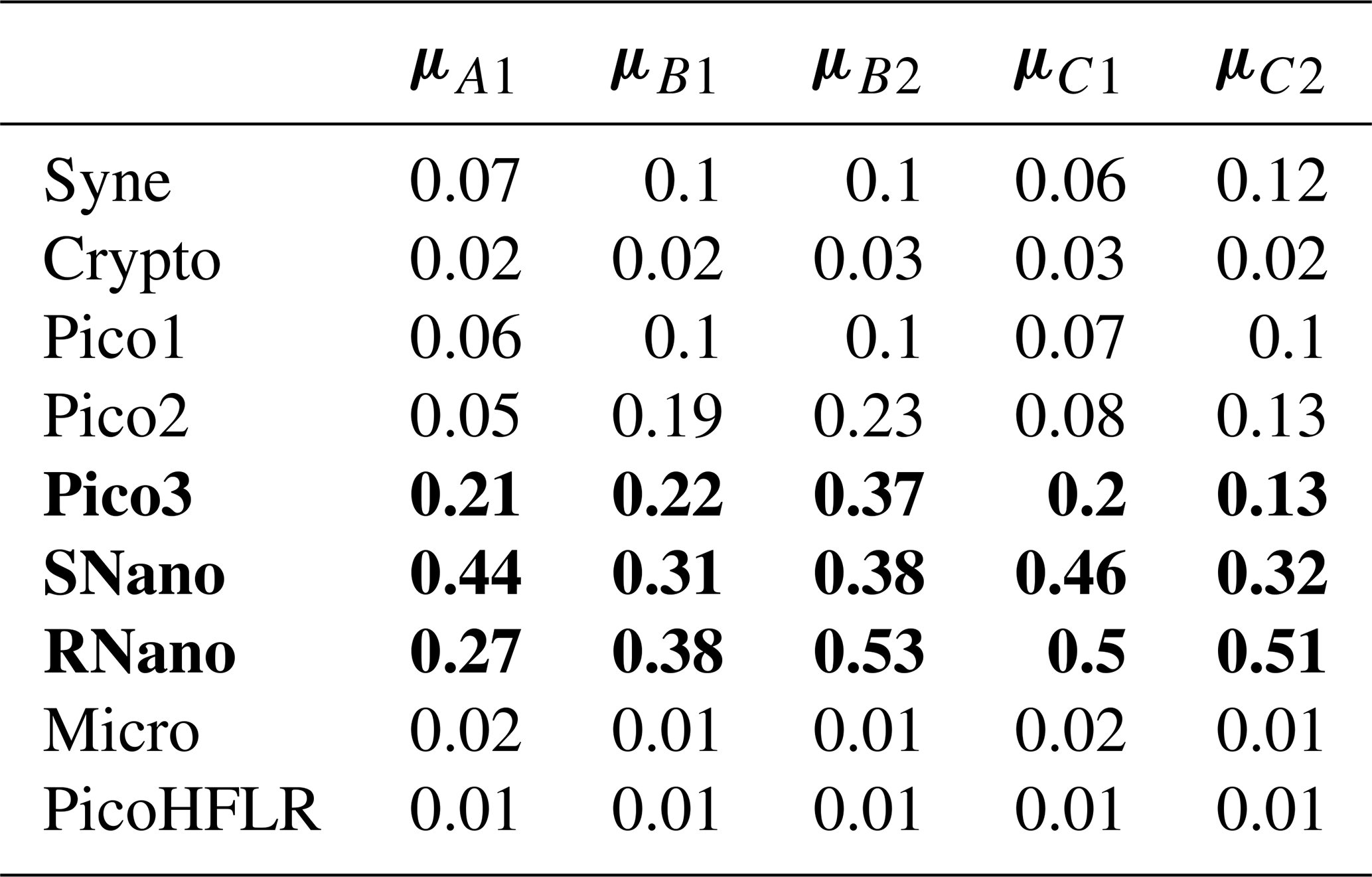
Table 2 Rounded μ (mmol C m⁻³) values estimated by Expectation–Maximization algorithm for the components in Com^A (A1), Com^B (B1 and B2) and Com^C (C1 and C2). The rows in bold correspond to the three phytoplankton groups presenting the highest μ values (i.e. biomass) within a component. For a better comparison between components for the same phytoplankton groups see Fig. 6.

4.3 Characteristics of the phytoplankton communities

The parameters of the multivariate Gaussian estimated by the EM algorithm are referenced in Table 2 for μ parameters and in Tables A3–A7 for Σ covariance matrices. The μ values and the variances in the diagonal of the Σ matrices of SNano, RNano and Pico3 are the highest. These results highlight the dominance and a large variability in biomass of these phytoplankton groups during the cruise.

In Com^B, the covariance matrices Σ_B1 and Σ_B2 are diagonal. This suggests that the addition of interactions between phytoplankton groups would not have improved the modeling of Com^B. By contrast, for Com^A and Com^C, the covariance matrices is not diagonal which allow to model positive or negative interactions between each phytoplankton group. The covariances matrices Σ_C1 and Σ_C2 present similar patterns and highlight mostly the positive interactions of SNano and RNano with most of the phytoplankton groups, except for Pico3. In these two communities Pico3 and Pico2 have a negative interaction. Σ_A1 presents similar pattern than in Σ_C1 and Σ_C2, but the main differences are negative interactions of Syne and Crypto with SNano, RNano, Micro and PicoHFLR, and strong interactions between Pico3 and Crypto (positive) and PicoHFLR (negative).

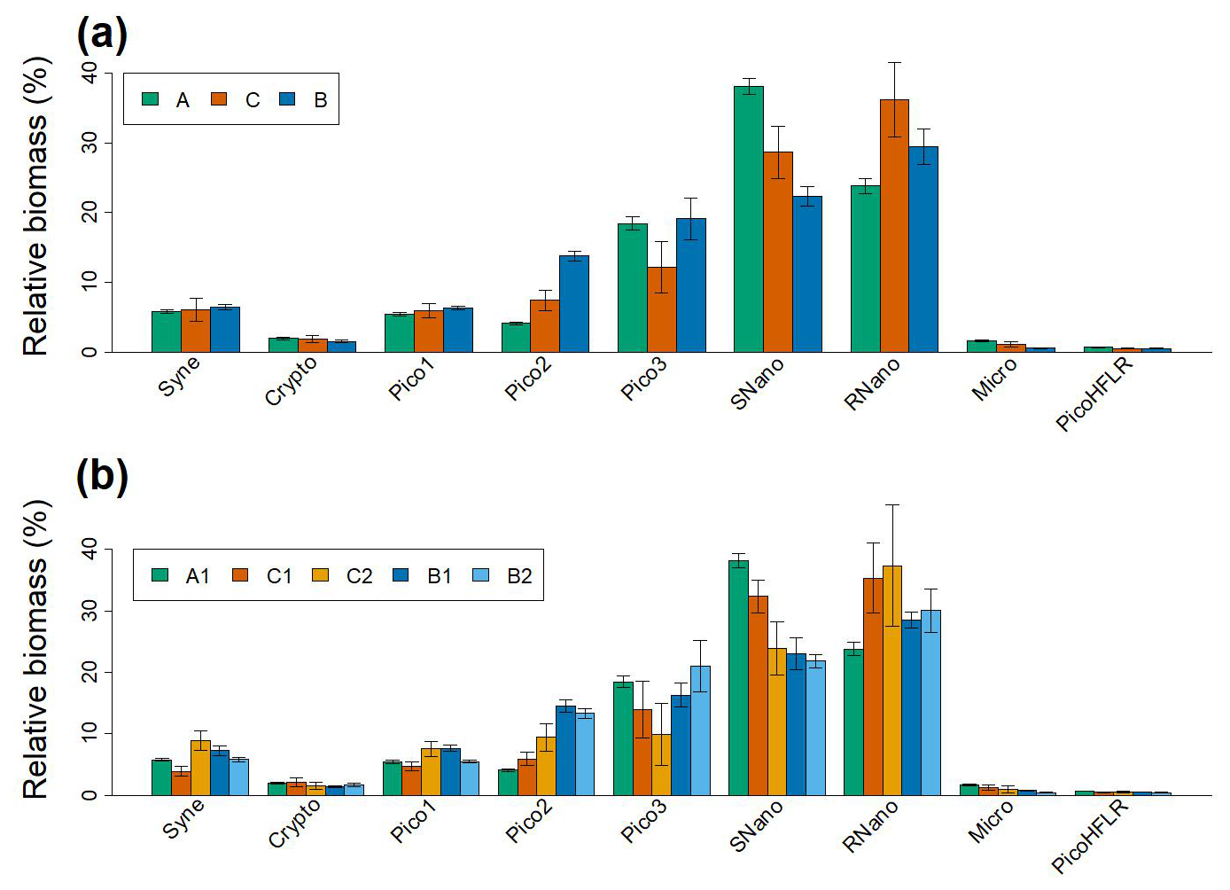
Figure 6 (a) Relative biomass (%) of the nine phytoplankton groups for the modeled communities Com^A, Com^B and Com^C. Biomass was calculated from μ values and weighted by α values of sub-components (for Com^B and Com^C). (b) Relative biomass (%) of the nine phytoplankton groups for the five sub-components. In (a) and (b) errors bars correspond to the 95 % confidence interval of the μ values.

Overall, the relative biomass (i.e. calculated from μ and α values) of the phytoplankton groups of Com^C is intermediate between Com^A and Com^B. However, RNano and Pico3 in Com^C show a relative biomass that is higher and lower, respectively than in Com^A and Com^B (Fig. 6a). This pattern is clearly observed when looking at the relative biomass at the sub-component scale (Fig. 6b). Where the relative biomass in C1 and C2 for RNano and Pico3 are, respectively higher and lower than in the other three components.Nevertheless, Fig. 6b, shows that two sub-components of the same community show different patterns for the same phytoplankton group. This is the case of C1 and C2 for Syne, which reach their lowest and highest relative biomass, respectively for these components.

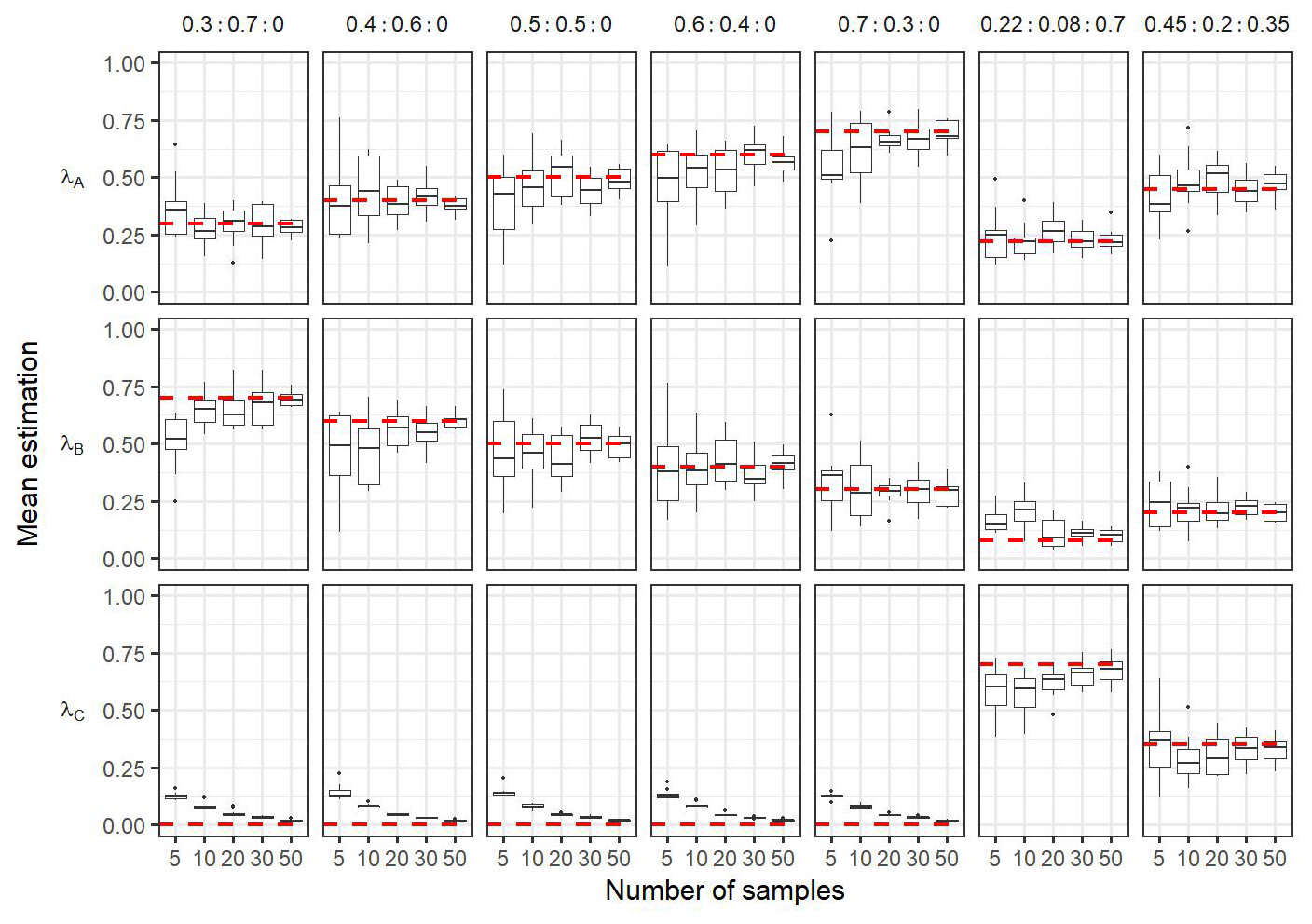
Figure 7 Boxplots of the mean of the posterior distributions during the sensitivity analysis. Each column correspond to the ${\mathit{\lambda }}_A:{\mathit{\lambda }}_B:{\mathit{\lambda }}_C$ estimation of a same condition: In the case frontal community is composed only by a mixture of adjacent water masses (i.e. λ_C=0) with varying proportion of simulated ${\mathit{\lambda }}_A:{\mathit{\lambda }}_B:{\mathit{\lambda }}_C$ (i.e. $\mathrm{0.3}:\mathrm{0.7}:\mathrm{0}$; $\mathrm{0.4}:\mathrm{0.6}:\mathrm{0}$; $\mathrm{0.5}:\mathrm{0.5}:\mathrm{0}$; $\mathrm{0.6}:\mathrm{0.4}:\mathrm{0}$; $\mathrm{0.7}:\mathrm{0.3}:\mathrm{0}$). The two last columns correspond to simulations where frontal community includes a new community Com^C (λ_C≠0), here the proportion used for simulations are the same as observed in the in situ dataset (i.e. λ_A=0.22, λ_B=0.08, λ_C=0.7) and $\mathrm{0.45}:\mathrm{0.2}:\mathrm{0.35}$. The dashed red horizontal lines correspond to the true λ values used to simulate the data in the mixtures. In each conditions the number of observations in the simulated data in the front varies from 5 to 50. Each boxplot is based on the 10 values of the mean calculated on the 10 simulated datasets for a same hypothesis and a same number of observations.

4.4 Sensitivity analysis of the Bayesian inference

Figure 7 shows the results of the sensitivity analysis performed on simulated data. The posterior distribution obtained from the Bayesian inference showed satisfactory mean estimation of the unknown parameters, leading to close estimates compared to the true values independently of the number of simulated observations. Note that while the average values of the posterior distributions of estimated parameters are reliable even for the lowest number of observations, increasing the number of simulated data lead to a decrease in the standard deviation of the posterior distribution (see in Fig. A6). In the case that the simulated data is only coming from a mixture of components Com^A and Com^B (λ_C=0), the sensitivity test shows that the estimated values of λ_C are very close to 0, meaning that this component is not important in the mixture (comparing to the cases where λ≠0) (Fig. 7). In addition, the model can detect slight changes in the proportions of components even in the case that the simulated data is coming from a mixture of the three components Com^A, Com^B and Com^C. Overall, the sensitivity analysis highlighted the robustness of the approach, even with fewer observations than the actual number of observations in the in situ data. Finally, the comparison test for equal distribution (Székely and Rizzo, 2004) between transitional waters and front rejected the H0 hypothesis ($H\mathrm{0}:T\stackrel{\mathrm{d}}{=}F$, p value < 0.05), which suggests that frontal and transitional water communities are different.

5 Discussion

5.1 A new approach to identify the frontal community

We developed a statistical approach to address key challenges in detecting and confirming fine-scale frontal-adapted phytoplankton communities, despite the limited and highly variable data from an oceanographic campaign. We represented the phytoplankton biomass distribution across and within a frontal region – reflecting the phytoplankton community composition – using a multivariate Gaussian mixture of distinct sub-communities. The critical objective was to determine which community and sub-community has the highest weight within the front. Here, we combined two approaches, Expectation–Maximization (EM) algorithm and Bayesian modelling, to characterize the nature of frontal phytoplankton communities from sparse in situ data. The EM algorithm allowed us to estimate parameters (μ and Σ) of Gaussian distributions and identify the number of communities and sub-communities (from relatively large datasets), while the Bayesian approach, known to be robust even with few observations, enabled us to determine their relative weights (λ and α) within the frontal community. Sensitivity analysis (Fig. 7) confirmed that the Bayesian inference was robust even for fewer observation (here down to 5) than the actual in situ frontal dataset (i.e. 11 observations).

The parameters μ (average biomass) and Σ (variance and covariance) provided a realistic overview of the phytoplankton community composition (PCC), highlighting the global dominance of two nanophytoplankton groups (SNano, RNano) and the largest picoeukaryote (Pico3), as well as the interactions between these groups that shape specific PCC (Tables 2, A3, A6, and A7). In the Mediterranean Sea, Synechococcus species (Syne) are the most dominant group of phytoplankton in abundance (Moutin et al., 2002). However, certain physical forcings, such as frontal structuring, may alter their presence by locally modifying environmental conditions (e.g., nutrient inputs), which can favor larger cells (Siokou-Frangou et al., 2010). In frontal zones, different types of interactions between plankton organisms, such as shading or shared predation, can lead to distinct community structures (Mangolte et al., 2022). Notably, the differences observed between the covariance matrices (i.e. Σ_A1, Σ_C1, and Σ_C2) suggest that interactions between phytoplankton are different within distinct communities (Tables A3, A6, and A7). Estimated values of parameters λ corresponding to the weight of communities within the front and its adjacent water masses provided information to answer our questions: “What is the structure of the community that might be formed at the front? Is the frontal community a mixture, where the expected community results from the combination of the adjacent water communities, or is there another community resulting from intrinsic frontal characteristics?”. In particular, λ_C (0.714 in the final model, Fig. 4c) represents the proportion of the frontal community attributed to Com^C. Since λ_C>0, our results suggest that the phytoplankton frontal community is not a mixture of adjacent communities, but instead is a specific frontal-adapted community. More precisely, λ_C indicates that Com^C represents more than 70 % of the frontal community Com^F (Fig. 4c).

Figure 8 shows the spatial projection of each sample point, with shapes and colors representing their community and sub-community classification, identified as the dominant component and sub-component of the Gaussian mixtures (highest λ and α). We reach two key conclusions. First, our approach successfully reconstructed the initial pattern observed by Tzortzis et al. (2021), characterized by a distribution of two communities on either side of the frontal region (here identified as Com^A and Com^B). A notable refinement was the identification of two sub-communities within Com^B (B1 and B2), which could be attributed to significant fine-scale meandering activity in the southern part of the front (i.e., within the Algerian Basin) (Millot, 1999). We hypothesize that such dynamics could lead to a closer cohabitation of different sub-communities. Second, our approach appeared to successfully detect the presence of the unknown Com^C located within the frontal community (Com^F).

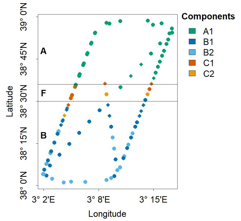
Figure 8 Spatial distribution of dominant components within the NS-Hippodrome. Dots are colored according to the multivariate Gaussian component, i.e. sub-communities (A1, B1, B2, C1 and C2) that reach the highest density (in nine dimension) for the sample phytoplankton groups observed biomass. The horizontal black lines correspond to the frontal area (latitude between 38.5 and 38.6°N, as in Fig. 1c, Component A1 (A community) was mostly dominant in the North of the Hippodrome. Components B1 and B2 (B sub-communities) were mostly dominant in the south of the Hippodrome. Components C1 and C2 (unknown C sub-communities) are mostly dominant in the front. Note that diamond shaped points correspond to samples transitional waters, T, that were not taken into account during the characterisation of the phytoplankton nine communities.

5.2 Phytoplankton communities across frontal areas

Our findings suggest that the frontal region acted as a selective environment, structuring phytoplankton communities by promoting certain phytoplankton groups while disadvantaging others (Fig. 6). According to our results, the frontal zone during PROTEVSMED-SWOT represented a narrow habitat for communities C1 and C2.

Mangolte et al. (2022) described the impact of frontal responses of plankton groups using the terms “winners” and “losers”. In the Californian Current Ecosystem, larger phytoplankton (e.g., microphytoplankton, diatoms) were classified as “winners” (increased abundance within fronts) and smaller picophytoplankton as “losers” (decreased abundance within fronts). Taking into account the whole Com^C, our result showed that RNano was clearly a “winner” and Pico3 was a “loser” within the front (Fig. 6). However, at a smaller scale, we showed that even within a same community, phytoplankton assemblage were different. For example, this was the case of Synechococcus (Syne) that, respectively showed the lowest and highest μ values with C1 and C2 (Fig. 6b). This suggests that Syne can simultaneously be both “winner” and “loser”, depending on local conditions. This pattern may result from differences in the origins of C1 and C2 communities, driven by advection or stirring of distinct water masses, or from biological interactions that either favored or hindered Syne (Lévy et al., 2018; Hernández-Hernández et al., 2020, 2021). Mangolte et al. (2023) highlighted that different plankton communities can be observed at a smaller scale (1–5 km) than the width of the front scale (10–30 km).

5.3 Limitations

The strong assumption that the potential front-adapted community existed within the outside dataset implies two limitations. On the one hand, the outside dataset is not an exhaustive dataset of the region. Actually, phytoplankton communities of the southern water masses may not be efficiently represented in the outside dataset, since the water masses off the Algerian coast (south of the sampling area) were not sampled. In addition, the inclusion of the stations close to the Balearic coasts might have led to an over-representation of coastal phytoplankton communities (different than the one observed in the open sea). But excluding coastal stations and selecting only data near the NS-Hippodrome transect (e.g., between 38–39° N and 3–5° E) did not drastically affect our results. On the other hand, frontal conditions could be unique in both space and time and might have not been sampled elsewhere than in the NS-Hippodrome transect. Actually, the communities identified in Com^C, C1 and C2, were mostly observed in stations in the same range of temperature and salinity that were close to the studied front, to the east, and were sampled a few days before the NS-Hippodrome transect sampling (Fig. A7). Hydrodynamic circulation across the frontal area was eastward (Tzortzis et al., 2021). This suggests that the communities observed at these sites in the outside dataset may have been advected from the front.

As Fig. 5 shows, our approach may not precisely capture the biomass distribution of certain phytoplankton groups (e.g. Pico3 and RNano). This is certainly because no biomass distributions that better fit the frontal data were observed in the “outside” dataset for these two groups. A more flexible option would be to estimate all parameters using a full Bayesian approach (i.e. the number of Gaussian components, μ, α, Σ and λ). However, as the number of parameters to be estimated far exceeded the actual number of observations at the front (number of observations = 11; number of parameters = 458), we opted to “fix” certain parameters (i.e. μ and Σ) using existing data (adjacent water masses and outside dataset). Nevertheless, the sensitivity analysis demonstrated the robustness of our approach, showing that the new components C1 and C2 in Com^C helped to model the community in the front more accurately, revealing the existence of a new frontal community.

6 Conclusions and perspectives

The re-analysis of the phytoplankton dataset from PROTEVSMED-SWOT using a novel statistical methodology allowed us to reveal a biological signal that remained undetected with classical statistical approaches due to the critical lack of data. This method effectively addresses one of the main challenges in in situ biological oceanography: the difficulty of collecting comprehensive datasets that integrate biological, physical, and biogeochemical measurements while maintaining high temporal and spatial resolution. Notably, without incorporating explicit spatial information or environmental variables into our analysis, our approach successfully captured the structuring effect of the front and detected the presence of a frontal-adapted phytoplankton community.

Importantly, our method reshaped our understanding of this moderately energetic front, previously considered merely a hydrodynamic barrier between two communities (Tzortzis et al., 2021). Instead, our results suggest that this front acted as a unique ecological environment where a distinct community seemed to have emerged. This study can be seen as a first attempt to assess this hypothesis, but due to the dataset scarcity, our results needs further application on other in situ datasets to be generalizable. Thus, given the broad applicability of our methodology to plankton datasets, we plan to use it to further investigate whether fronts generally function as simple boundaries or as areas fostering the development of frontal-adapted communities. In addition, recent work has shown that frontal conditions appear to favor the presence of non-dominant phytoplankton groups relative to dominant ones (, ). Such a “refuge effect” will be evaluated in further research that will analyse satellite-based data sets (e.g., ocean color and altimetry) to provide a global perspective on phytoplankton distribution in frontal regions. Additionally, the future research will include analyses of other in situ larger plankton datasets, such as those from BioSWOT-Med (Doglioli et al., 2024), which provide a more comprehensive environmental context. Including the complete dataset from BioSWOT-Med, integrating nutrient concentrations and fluxes, as well as zooplankton concentrations and grazing rates, will help disentangle the key processes driving the observed phytoplankton community composition.

Appendix A

Table A1 Summary of the statistics (mean, standard deviations, quantiles 2.5, 25, 50, 75 and 97.5 % of the posterior distributions) and convergence metrics (effective sample size ESS, and $\widehat{R}$) of the estimated parameters of the explanatory model.

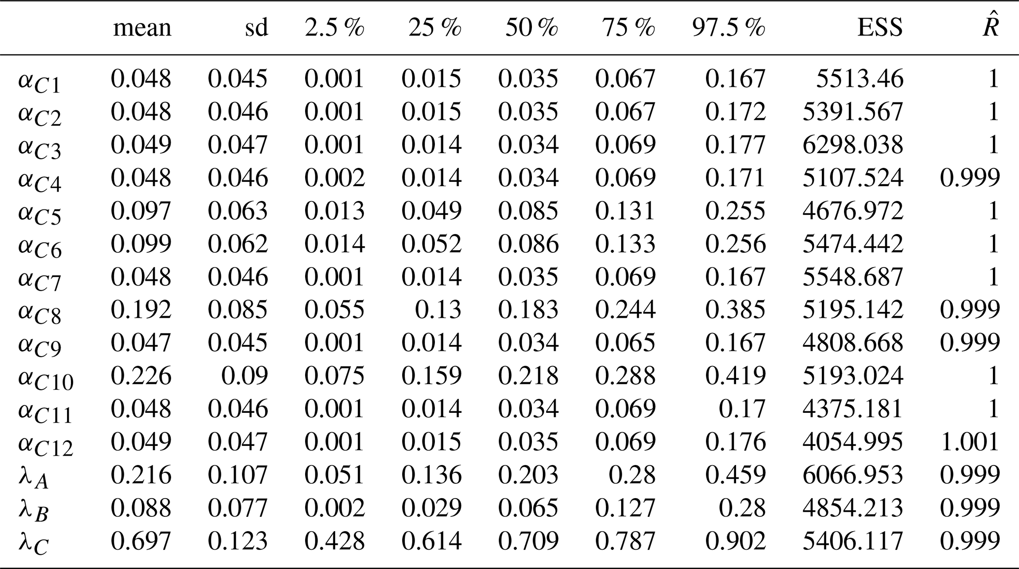
Table A2 Summary of the statistics (mean, standard deviations, quantiles 2.5, 25, 50, 75 and 97.5 % of the posterior distributions) and convergence metrics (effective sample size ESS, and $\widehat{R}$) of the estimated parameters of the final model.

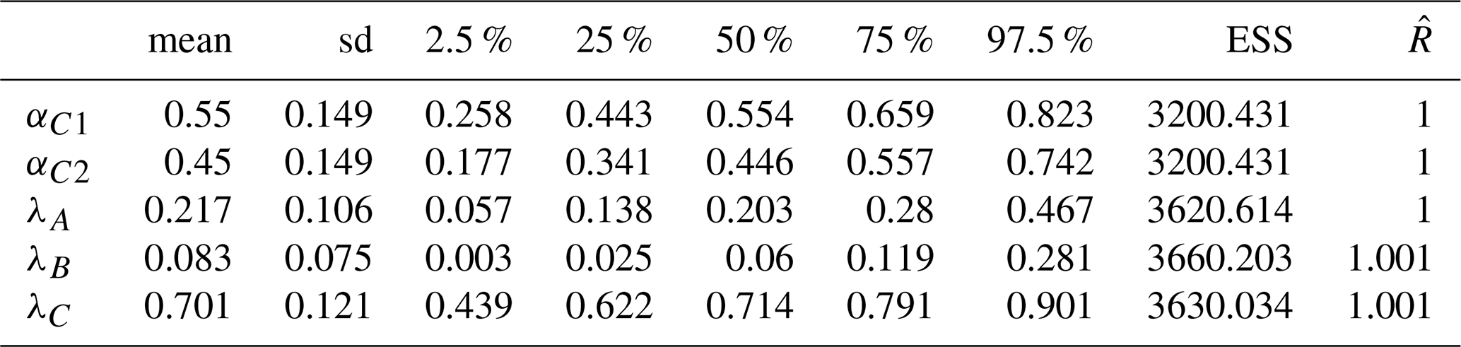
Table A3 Σ covariance matrix estimated by Expectation–Maximization algorithm for the component A1 in Com^A.

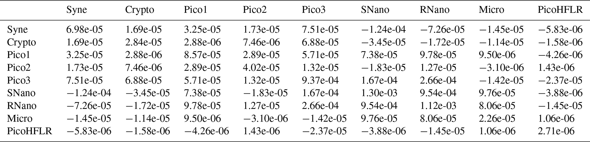
Table A4 Σ covariance matrix estimated by Expectation–Maximization algorithm for the component B1 in Com^B.

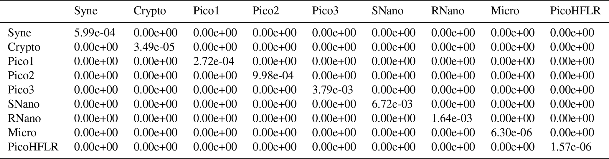
Table A5 Σ covariance matrix estimated by Expectation–Maximization algorithm for the component B2 in Com^B.

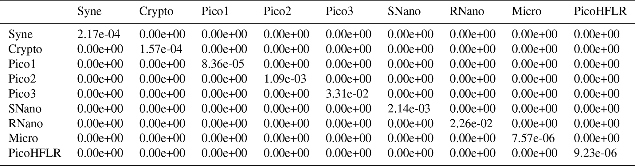
Table A6 Σ covariance matrix estimated by Expectation–Maximization algorithm for the component C1 in Com^C.

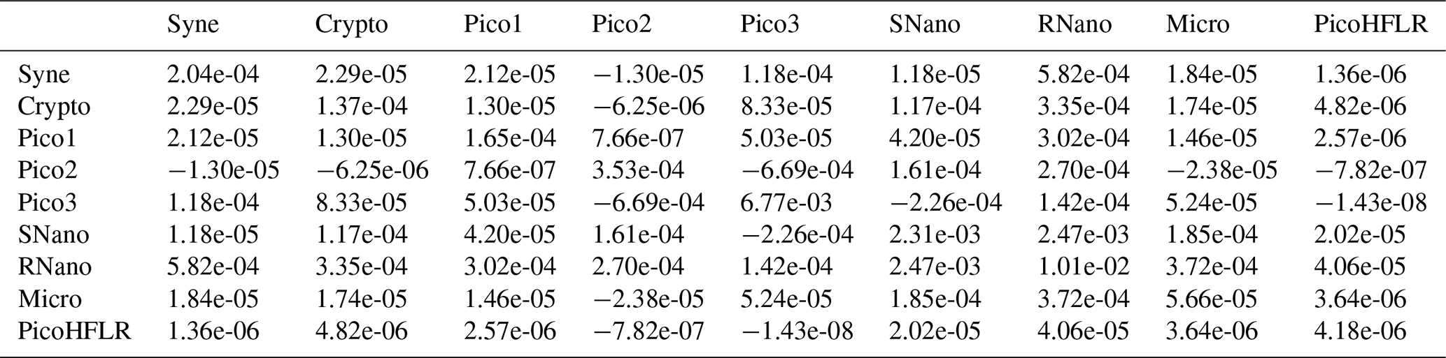
Table A7 Σ covariance matrix estimated by Expectation–Maximization algorithm for the component C2 in Com^C.

Figure A1 Variation of the salinity measurements during the cruise between 11 and 13 May. The horizontal lines correspond to the isohalines that were chosen to characterize the frontal area. Green dots correspond to the water mass A, blue dots to the water mass B. Within the frontal area, latitudinal limits were chosen according to Tzortzis et al. (2021). In this zone, orange dots correspond to the front, and grey crosses to the transitional waters, T, that are not taken for the data analyses.

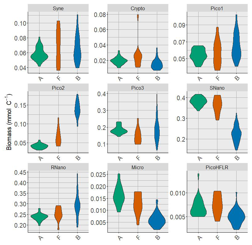
Figure A2 Violin plot of the phytoplankton groups biomass in the three water masses A, F and B. Biomasses are expressed in mmolC m⁻³.

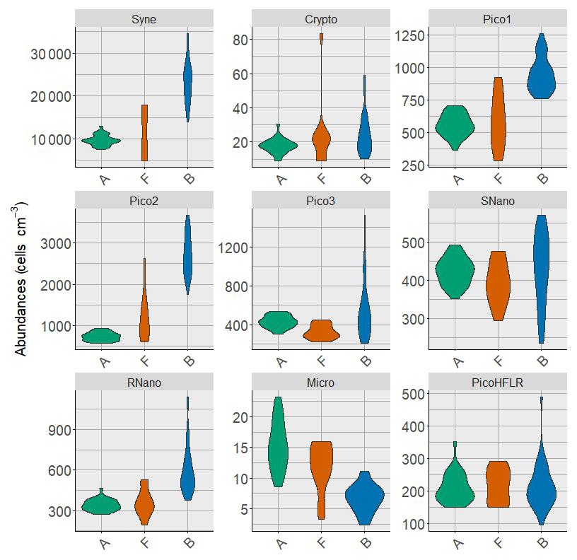
Figure A3 Violin plot of the phytoplankton groups abundances in the three water masses A, F and B. Abundances are expressed in cells cm⁻³.

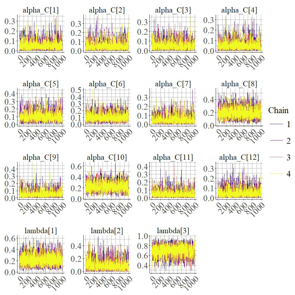
Figure A4 Trace of the posteriors distributions of the parameters estimated by the first Bayesian model, exploratory model.

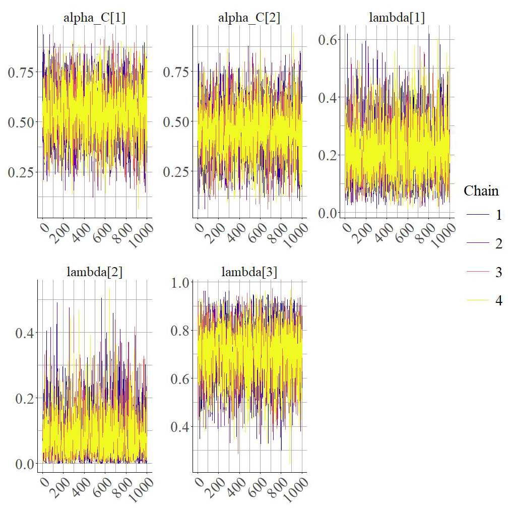
Figure A5 Trace of the posteriors distributions of the parameters estimated by the second Bayesian model, final model.

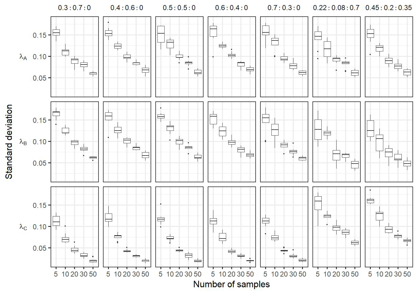
Figure A6 Boxplots of the standard deviation of the posterior distributions of the sensitivity analysis. Each column correspond to the ${\mathit{\lambda }}_A:{\mathit{\lambda }}_B:{\mathit{\lambda }}_C$ estimation of a same condition: In the case frontal community is composed only by a mixture of adjacent water masses (i.e. λ_C=0) with varying proportion of simulated ${\mathit{\lambda }}_A:{\mathit{\lambda }}_B:{\mathit{\lambda }}_C$ (i.e. $\mathrm{0.3}:\mathrm{0.7}:\mathrm{0}$; $\mathrm{0.4}:\mathrm{0.6}:\mathrm{0}$; $\mathrm{0.5}:\mathrm{0.5}:\mathrm{0}$; $\mathrm{0.6}:\mathrm{0.4}:\mathrm{0}$; $\mathrm{0.7}:\mathrm{0.3}:\mathrm{0}$). The two last columns correspond to simulations where frontal community includes a new community Com^C (λ_C≠0), here the proportion used for simulations are the same as observed in the in situ dataset (i.e. λ_A=0.22, λ_B=0.08, λ_C=0.7) and $\mathrm{0.45}:\mathrm{0.2}:\mathrm{0.35}$. The dashed red horizontal lines correspond to the true λ values used to simulate the data in the mixtures. In each conditions the number of observations in the simulated data in the front varies from 5 to 50. Each boxplot is based on the 10 values of the mean calculated on the 10 simulated datasets for a same hypothesis and a same number of observations.

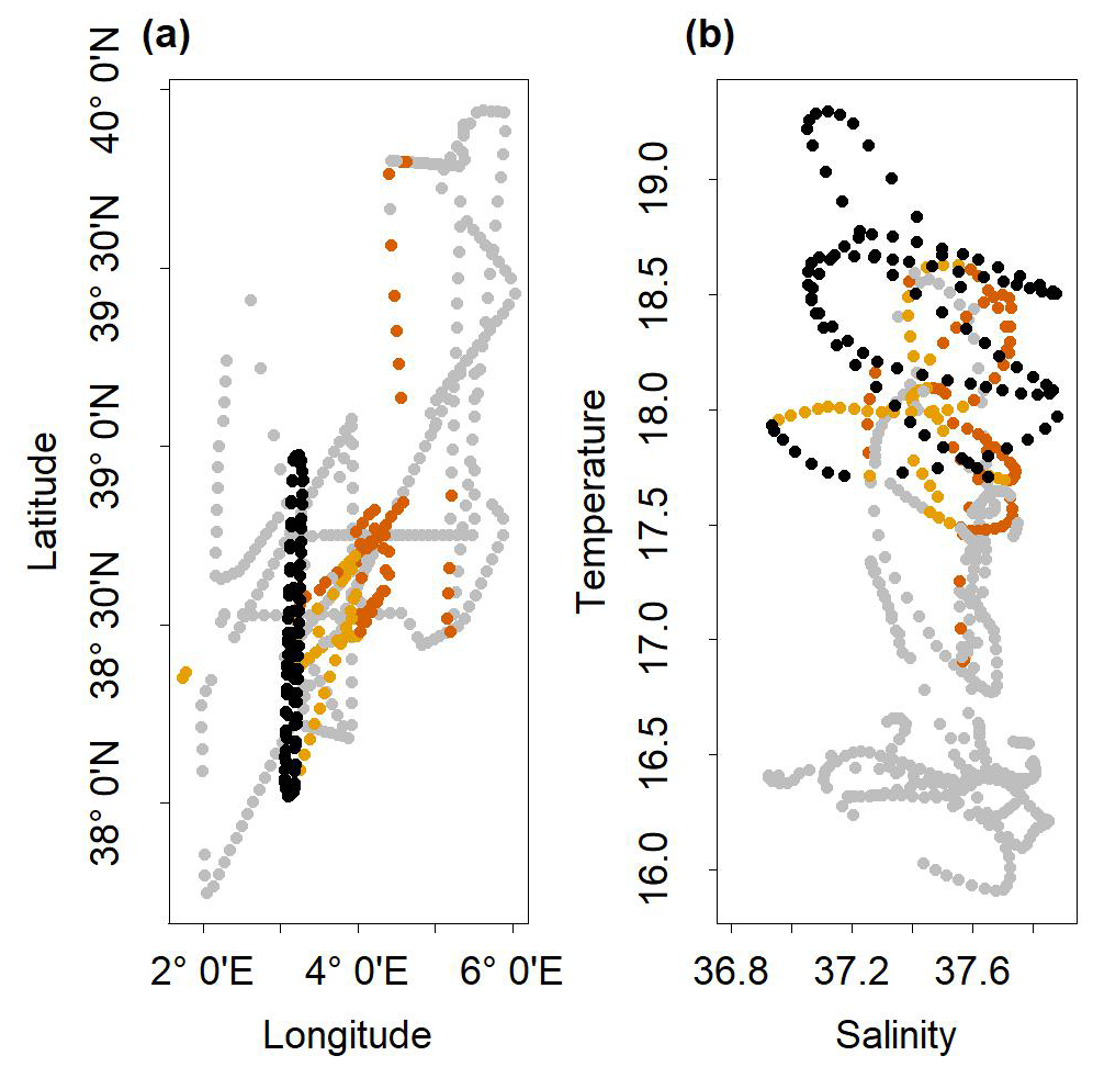
Figure A7 (a) Spatial Distribution of stations belonging to cluster C1 (in dark orange), cluster C2 (in orange) and the NS-Hippodrome transect stations (in black). The grey dots are the others stations of the cruise. (b) Temperature/Salinity diagram of the stations of the cruise. The dots in dark orange correspond to cluster C1, in orange to cluster C2, in black to the NS-Hippodrome transect stations, and in grey are the others stations of the cruise.