On computing the maximum likelihood estimates for the q-Pareto distribution and application to earthquakes

We define a generalized exponential distribution (G-ED) that overlaps with a generalized Pareto distribution (GPD). Then, we introduce the q-Pareto distribution (q-PD) with two-parameter family distribution (strict positive shape and scale parameters) via transforming the G-ED. We demonstrate that the q-PD can be used to model the exceedances over a threshold, and we focus to estimate the q-PD parameters. Often, the estimation is taken the maximum likelihood estimation (MLE) because have a consistent estimator with an asymptotic normal distribution and is asymptotically effective in many cases. We present an algorithm to compute the MLE for q-PD parameters with confidence intervals for each estimator. Numerical examples are given to illustrate the results obtained. Efficient numerically methods are developed for the MLE of the q-PD parameters to maximize the log-likelihood of the q-PD.

1 Introduction

In probability theory and statistics, the exponential distribution family and the Pareto distribution family, each of them is a parametric set of probability distributions of a certain form, in terms of normal parameters, and to determine useful sample statistics. Hence, the exponential distribution is not the same as the class of families of exponential distributions, but rather it is one of the distributions of this family, which includes several distributions, including: normal, gamma, chi-squared, Poisson etc. Also, the Pareto distribution has many related distributions known as Pareto Type I, II, III, IV etc., and Pareto Type IV contains Pareto Type I–III as special cases. So, it can be said that we have two families of important distributions. Each of them has many applications in many fields. The cumulative distribution function (cdf) of the Pareto distribution parameters (Type I) is given by

$$\begin{array}{}\text{(1)}& G_{t,\mathit{\alpha }}\left(x\right):=\left\{\begin{array}{ccc}\mathrm{1}-{\left(\frac{t}{x}\right)}^b& \text{for}& x\ge t\\ \mathrm{1}& \text{for}& x<t\end{array}\right.,\end{array}$$

It follows under differentiation that the probability density function (pdf) of a Pareto random variable with parameters b and t is:

$$g_{t,b}\left(x\right):=\left\{\begin{array}{ccc}\frac{a{t}^b}{x^{b+\mathrm{1}}}& \text{for}& x\ge t\\ \mathrm{0}& \text{for}& x<t\end{array}\right.,$$

with $x\in [\mathrm{0};{\mathit{\tau }}_{G_{t,b}}[$ where ${\mathit{\tau }}_{G_{t,b}}=\sup \left\{x:G_{t,b}\left(x\right)<\mathrm{1}\right\}\le \mathrm{\infty }$ denotes the upper endpoint of G_t,b and b is a positive parameter called the Pareto index or the shape parameter. Likewise, the cdf of the exponential distribution parameter is given by

$$\begin{array}{}\text{(2)}& H_b\left(x\right):=\left\{\begin{array}{ccc}\mathrm{1}-\exp \left(-bx\right)& \text{for}& x\ge \mathrm{0}\\ \mathrm{0}& \text{for}& x<\mathrm{0}\end{array}\right.,\end{array}$$

It that the pdf of the exponential distribution random variable with parameter b>0 is:

$$h_b\left(x\right):=\left\{\begin{array}{ccc}b\exp \left(-bx\right)& \text{for}& x\ge \mathrm{0}\\ \mathrm{0}& \text{for}& x<\mathrm{0}\end{array}\right.,$$

There are distributions related to the Pareto distribution used to model the energy released by large earthquakes, such as: log-Pareto, Extended Slash Pareto, Tapered Pareto, Generalized Pareto Distribution (GPD), among others. There are some transformations that allow the Pareto distribution to be linked to other distributions like: the Burr distribution, the Power functions, the Chi-square distributions etc. Also, the Pareto distribution has many uses for modeling many types of heavy-tailed distribution. de la Barra and Vega-Jorquera (2021) proposed a new probability distribution related to the Pareto distribution, which is the q-Pareto distribution (q-PD) by transforming the q-exponential distribution. The q-PD is highly effective for modelling the magnitudes of larger, extreme earthquakes in global catalogues, where a small change in parameters results in exponential changes in seismic moments. Also, is used in insurance and actuarial statistics to analyse extreme events, such as calculating reinsurance premiums for catastrophic losses.

Notice that, Tsallis (1994) introduced the q-logarithmic function for x>0. He has proven that the logarithmic function can be generalized to a function of fractional power by

$$\begin{array}{}\text{(3)}& {\ln }_q\left(x\right):=\left\{\begin{array}{ccc}\ln \left(x\right)& \text{if}& q=\mathrm{1}\\ \frac{x^{\mathrm{1}-q}-\mathrm{1}}{q-\mathrm{1}}& \text{if}& q\ne \mathrm{1}\end{array}\right.,\end{array}$$

With q is a fixed real number. Among the properties of the q-logarithmic function which is defined in Eq. (3), we mention:

1. ln_q(1)=0

2. $\frac{\partial {\ln }_q\left(x\right)}{\partial x}=x^{-q}$

3. The q-logarithmic function is a concave function.

4. exp_q(ln_q(x))=x for all x>0 with exp_q is the inverse function of ln_q which given as

   $$\begin{array}{}\text{(4)}& {\exp }_q\left(x\right):=\left\{\begin{array}{ccc}\exp \left(x\right)& \text{if}& q=\mathrm{1}\\ {\left(\mathrm{1}+\left(\mathrm{1}-q\right)x\right)}^{\frac{\mathrm{1}}{\mathrm{1}-q}}& \text{if}& q\ne \mathrm{1}\end{array}\right.,\end{array}$$

   and the basic properties of exp_q are exp_q(0)=1 and $\frac{\partial {\exp }_q\left(x\right)}{\partial x}={\left({\exp }_q\left(x\right)\right)}^q$. Also, exp_q, called the q-exponential function is a convex function when q>0. Also, for b>0 and under $q=\mathrm{1}-\frac{\mathrm{1}}{n}$ we have that

   $$\underset{n\to +\mathrm{\infty }}{\lim }{\left(\mathrm{1}-\left(\mathrm{1}-q\right)bx\right)}^{\frac{\mathrm{1}}{\mathrm{1}-q}}=\exp \left(-bx\right)={\stackrel{\mathrm{‾}}{H}}_b\left(x\right)$$

   where ${\stackrel{\mathrm{‾}}{H}}_b$ is the tail-exponential distribution random which is defined in Eq. (2). Then, for b>0 and $\mathrm{1}-\left(\mathrm{1}-q\right)bx>\mathrm{0}$ we have $x<\frac{\mathrm{1}}{\left(\mathrm{1}-q\right)b}$ if $\mathrm{0}<q<\mathrm{1}$ and $x>\frac{\mathrm{1}}{\left(\mathrm{1}-q\right)b}$ if q>1. And we agree that exp_q(−bx) is the general exponential (G-exponential) function or the q-exponential function which given by

   $$\begin{array}{}\text{(5)}& {\exp }_p\left(-bx\right)=\begin{array}{ccc}{\left(\mathrm{1}-\left(\mathrm{1}-q\right)bx\right)}^{\frac{\mathrm{1}}{\mathrm{1}-q}}& \text{if}& q\ne \mathrm{1}\end{array},\end{array}$$

Since b>0 with $q\in {\mathbb{R}}_{+}^{*}-\left\{\mathrm{1}\right\}$ and ${\exp }_q\left(-bx\right)>\mathrm{0}$ has the same properties as the function exp(−bx) such as continuity and derivation for x>0 and ${\exp }_q\left(-bx\right)=\mathrm{1}$ as $x\to +\mathrm{\infty }$. Through, the relation of the tail-exponential distribution which is defined in Eq. (2) and the q-exponential function in Eq. (5) we define the cdf of the q-exponential distribution (G-exponential distribution (G-ED)) which is presented in Eq. (2) if q≠1 as

$$\begin{array}{}\text{(6)}& H_{q,b}\left(x\right):=\mathrm{1}-{\left(\mathrm{1}-\left(\mathrm{1}-q\right)bx\right)}^{\frac{\mathrm{1}}{\mathrm{1}-q}},\end{array}$$

Also, by deriving the cdf H_q,b, we can define the pdf in the form

$$h_{q,b}\left(x\right):=b{\left(\mathrm{1}-\left(\mathrm{1}-q\right)bx\right)}^{\frac{q}{\mathrm{1}-q}},$$

where $q\in {\mathbb{R}}_{+}^{*}-\left\{\mathrm{1}\right\}$ and b is a positive scale parameter for $x\in [\mathrm{0};{\mathit{\tau }}_{H_{q,b}}[$ with ${\mathit{\tau }}_{H_{q,b}}=\frac{\mathrm{1}}{b\left(\mathrm{1}-q\right)}$ if $\mathrm{0}<q<\mathrm{1}$. And ${\mathit{\tau }}_{H_{q,b}}=\mathrm{\infty }$ if q>1 where ${\mathit{\tau }}_{H_{q,b}}=\sup \left\{x:H_{q,b}\left(x\right)<\mathrm{1}\right\}\le \mathrm{\infty }$ denote the upper endpoint of H_q,b.

In addition, we have H_q,b in Eq. (6) recover the exponential distribution in Eq. (2) as q→∞ that's why we note that the G-ED in Eq. (6) is a generalization of the exponential distribution in Eq. (2). We point out that, there are those who presented a generalization of the exponential distribution that differs from what we saw in this work. For an instant, you can see the article presented by Gupta and Kundu (2007). The q-exponential function arises as a distribution that maximizing the Tsallis entropy under constraints, acting as a non-standard “exponential” for complex systems. Previous studies extensively explore q-exponential and Tsallis entropy distributions which is generalizes Boltzmann-Gibbs entropy as powerful tools for complex systems, moving beyond standard Boltzmann-Gibbs stats, finding applications in many fields such as: physics (particle/nuclear, geomagnetic, super-statistics), the finance (risk modeling), seismology (earthquake patterns), and information theory. This reveals latent power-law behaviors and self-organization, and providing unified frameworks for non-equilibrium phenomena through their q-parameter, which generalizes standard exponential functions.

We consider $Y_{\mathrm{1}},\mathrm{\dots },Y_n$ be a sequence of iid rv's from the G-ED which is given in Eq. (6) (Note, $Y\sim H_{q,b}$) and consider the random variable (rv) X as

$$\begin{array}{}\text{(7)}& X=t{e}^Y\text{then}Y=\log \left({\displaystyle \frac{X}{t}}\right)\text{for}X>t,\end{array}$$

And we simply can know the explicit expression to distribute if rv X by

$$\begin{array}{}\text{(8)}& \begin{array}{rl}P\left(X\le x\right)& =P\left(t{e}^Y\le x\right)=P\left(Y\le \log \left({\displaystyle \frac{x}{t}}\right)\right)\\ & =H_{q,b}\left(\log \left({\displaystyle \frac{x}{t}}\right)\right),\end{array}\end{array}$$

So, we present the approach of the cdf of the q-PD by

$$\begin{array}{}\text{(9)}& F\left(x\right)=\mathrm{1}-{\left(\mathrm{1}+\left(q-\mathrm{1}\right)b\log \left({\displaystyle \frac{x}{t}}\right)\right)}^{\frac{-\mathrm{1}}{q-\mathrm{1}}},\end{array}$$

which in differentiation yields,

$$\begin{array}{}\text{(10)}& f\left(x\right)={\displaystyle \frac{b}{x}}{\left(\mathrm{1}+\left(q-\mathrm{1}\right)b\log \left({\displaystyle \frac{x}{t}}\right)\right)}^{\frac{-\mathrm{1}}{q-\mathrm{1}}-\mathrm{1}}\end{array}$$

with b>0 and $t<x<t\exp \frac{-\mathrm{1}}{b\left(q-\mathrm{1}\right)}$ if $\mathrm{0}<q<\mathrm{1}$ and $x>t\exp \frac{-\mathrm{1}}{b\left(q-\mathrm{1}\right)}$ if q>1. Therefore $Y\sim H_{q,b}$ then X ∼ q-PD where X=te^Y with X>t. Then, the G-ED and q-PD are related by an exponential expression. And, the q-PD in Eq. (9) and the G-ED in Eq. (6) are related by $F\left(x\right)=H_{q,b}\left(\log \left(\frac{x}{t}\right)\right)$ for x>t.

Recall de la Barra and Vega-Jorquera (2021) studied the q-PD and defined it by taking the sample $Y_{\mathrm{1}},\mathrm{\dots },Y_n$ to be a sequence of iid rv's following the cdf of the q-exponential distribution which has the df given in the following formula.

$$\begin{array}{}\text{(11)}& F_{q,b}\left(x\right)=\begin{array}{ccc}\mathrm{1}-{\left(\mathrm{1}-\left(\mathrm{1}-q\right)bx\right)}^{\frac{\mathrm{2}-q}{\mathrm{1}-q}}& \text{if}& q\ne \mathrm{1}\end{array}\end{array}$$

where $q\in ]\mathrm{0};\mathrm{1}[\cup ]\mathrm{1};\mathrm{2}[$ is the shape parameter and b>0 is the scale parameter. And the pdf of the q-exponential distribution is

$$f_{q,b}\left(x\right)=bx\left(\mathrm{2}-q\right){\exp }_q\left(-bx\right)$$

with $\mathrm{1}-\left(\mathrm{1}-q\right)bx>\mathrm{0}$ and $b\left(\mathrm{2}-q\right)>\mathrm{0}$ where exp_q(−bx) is the G-exponential function given in Eq. (5). For $\mathrm{0}\le x<{\mathit{\tau }}_{F_{q,b}}$; ${\mathit{\tau }}_{F_{q,b}}=\frac{\mathrm{1}}{b\left(\mathrm{1}-q\right)}$ with $\mathrm{0}<q<\mathrm{1}$ and ${\mathit{\tau }}_{F_{q,b}}=\mathrm{\infty }$ if $\mathrm{1}<q<\mathrm{2}$ for ${\mathit{\tau }}_{F_{q,b}}=\sup \left\{x:F_{q,b}\left(x\right)<\mathrm{1}\right\}\le \mathrm{\infty }$ denote the upper endpoint of F_q,b. Although we can find a relationship between the G-ED which is presented in Eq. (6) and the q-exponential distribution given in Eq. (11) as follows:

$$F_{q,b}\left(x\right)=H_{\mathit{\lambda },\mathit{\beta }}\left(x\right)\text{with}\mathit{\lambda }={\displaystyle \frac{\mathrm{1}}{q-\mathrm{2}}}\text{and}\mathit{\beta }=b\left(\mathrm{2}-q\right),$$

where $\mathit{\lambda }\in ]-\mathrm{\infty };-\mathrm{1}[\cup ]-\mathrm{1},-\mathrm{0.5}]$ and β>0 for $q\in ]\mathrm{0};\mathrm{1}[\cup ]\mathrm{1};\mathrm{2}[$ and b>0.

Fitting GED to the general Pareto distribution (GPD)

Moreover, considering the G-ED which is given in Eq. (6) and if we take $\mathit{\gamma }=\left(q-\mathrm{1}\right)$ with $q\in ]\mathrm{0};\mathrm{1}[\cup ]\mathrm{1};+\mathrm{\infty }[$ and $\mathit{\sigma }=\mathrm{1}/b$ with b>0. We find that the cdf H_q,b overlaps with the GPD parameters which his df define as

$$\begin{array}{}\text{(12)}& H_{\mathit{\gamma },\mathit{\sigma }}\left(x\right):={\left(\mathrm{1}+{\displaystyle \frac{\mathit{\gamma }}{\mathit{\sigma }}}x\right)}^{\frac{-\mathrm{1}}{\mathit{\gamma }}},\end{array}$$

with $\mathit{\gamma }\in ]-\mathrm{1};\mathrm{0}[\cup ]\mathrm{0};+\mathrm{\infty }[$ being the shape parameter and σ>0 the scale parameter. For q=1 we get γ=0 and $H_{\mathit{\gamma },\mathit{\sigma }}\left(x\right):=\mathrm{1}-\exp \left(-x/\mathit{\sigma }\right)$. Then the GPD's can be rewritten in terms of the G-exponential function which is presented in Eq. (5) as.

$$H_{\mathit{\gamma },\mathit{\sigma }}\left(x\right):=\left\{\begin{array}{ccc}\mathrm{1}-{\exp }_q\left(-bx\right)& \text{with}& q\ne \mathrm{1}\\ \mathrm{1}-\exp \left(-bx\right)& \text{with}& q=\mathrm{1}\end{array}\right.,$$

with $\mathit{\gamma }=\left(q-\mathrm{1}\right)$ and $\mathit{\sigma }=\mathrm{1}/b$ for q>0 and b>0. The interesting point is that GPD is used to model heavy-tailed distributions and has applications in many fields including: network traffic, hydrology, climatology, geophysics, materials science, etc. We note $\stackrel{d}{\to }$ convergence in distribution. These uses of GPD are related to the peak-over-threshold (POT) method, and the underlying rationale is, of course, the fact that Balkema and de Haan (1974) and Pickands (1975) assert for $X_{\mathrm{1}},\mathrm{\dots },X_n$ to be a sequence of independent and identically distributed (iid) random variables (rv's) from some unknown df F and if F satisfies the following condition:

$$\begin{array}{}\text{(13)}& P\left({\displaystyle \frac{X_{n,n}-A_n}{B_n}}\le x\right)\stackrel{d}{\to }\mathit{\varphi }\left(x\right),\end{array}$$

as n→∞ for x>0 with the sequences of constants A_n>0 , B_n>0 and $X_{n,n}=max\left(X_i\right)$ for $i=\mathrm{1},\mathrm{\dots },n$ and the df ϕ(x) is continuous. Then, there exists a normalizing function σ(t)>0 such that for all x>0,

$$\begin{array}{}\text{(14)}& \underset{t\to {\mathit{\tau }}_F}{\lim }\underset{\mathrm{0}<x<t-{\mathit{\tau }}_F}{\sup }\left|F_t\left(x\right)-H_{\mathit{\gamma },\mathit{\sigma }}\left(x\right)\right|=\mathrm{0},\end{array}$$

with γ∈ℝ and ${\mathit{\tau }}_F=\sup \left\{x:F\left(x\right)<\mathrm{1}\right\}\le \mathrm{\infty }$ denote the upper endpoint of F and F_t be the conditional df of X−t which is given as

$$\begin{array}{}\text{(15)}& F_t\left(x\right)=P\left(X<t+x|X>t\right)={\displaystyle \frac{F\left(x+t\right)-F\left(t\right)}{\mathrm{1}-F\left(t\right)}},\end{array}$$

with X>t and $\mathrm{1}-F\left(t\right)>\mathrm{0}$ for t<τ_F and x>0. Then under Eq. (14) it is well known F_t that up to scale and location transformations as the GPD which given in Eq. (12), $F_t\stackrel{d}{\to }{H}_{\mathit{\gamma },\mathit{\sigma }}$.

Theorem 1. Let $X_{\mathrm{1}},\mathrm{\dots },X_n$ be positive iid rv's with unknown common df F and $X_{\mathrm{1},n}\le \mathrm{\dots }\le X_{n,n}$ denote the order statistics correspondence. If the condition (14) is met then the tail joint df of $\left(X_{n-k,n},\mathrm{\dots },X_{n,n}\right)$ for X−t with X>t be the G-ED which is given in Eq. (6).

Proof of Theorem 1. For q>0 and b>0, if we take

$$\begin{array}{}\text{(16)}& q=\mathit{\gamma }-\mathrm{1}\mathit{and}b=\mathrm{1}/\mathit{\sigma }\left(t\right),\end{array}$$

Replace them in the GPD which defined in Eq. (12). Then, we find the limit in Eq. (14) becomes

$$\begin{array}{}\text{(17)}& \underset{t\to {\mathit{\tau }}_F}{\lim }\underset{\mathrm{0}<x<t-{\mathit{\tau }}_F}{\sup }\left|F_t\left(x\right)-H_{q,b}\left(x\right)\right|=\mathrm{0},\end{array}$$

with $q\in ]\mathrm{0};\mathrm{1}[\cup ]\mathrm{1};+\mathrm{\infty }[$ and b>0 where H_q,b is the G-ED which is presented in Eq. (6). End of proof.

Consequently, the limit (17) means that the df of excesses over a threshold F_t follows approximately a G-ED for large values of the threshold t>0 ($F_t\stackrel{d}{\to }{H}_{q,b}$).

There are many works that address the estimation of GPD parameters using a numerical algorithm based on the MLE method. Under Theorem 1 the G-ED is widely used in statistics to model extreme values and exceedances over a threshold. In this article, we will focus on the methodology employed by Kouider (2019b), and Kouider and Benatia (2023), and Kouider et al. (2023a, b) for estimating GPD parameters via the MLE. In order to propose a robust numerical algorithm for estimating the parameters of the q-PD.

2 The MLE for the q-PD

Recall that in this paper we consider the estimation (q,b) based on the MLE method using a numerical method in the form of an algorithm, which we will present in this section. To specify it, let $X_{\mathrm{1}},\mathrm{\dots },X_n$ be iid random variables with the common df F which is the cdf q-PD given in Eq. (9). Then for q>0 and b>0 with t>0 the likelihood function can be written as

$$\begin{array}{}\text{(18)}& \begin{array}{rl}& \mathrm{\ell }\left(C_i;q,b\right)=\\ & \left\{\begin{array}{cc}\prod _{i=\mathrm{1}}^n\frac{b}{X_i}{\left(\mathrm{1}+\left(q-\mathrm{1}\right)b\log \left(C_i\right)\right)}^{\frac{-q}{q-\mathrm{1}}}& \text{for}q\ne \mathrm{1}\\ \prod _{i=\mathrm{1}}^n\frac{b}{X_i}\exp \left(-b\log \left(C_i\right)\right)& \text{for}q=\mathrm{1}\end{array}\right.,\end{array}\end{array}$$

with $C_i=\frac{X_i}{t}$ for X_i>t and $i=\mathrm{1},\mathrm{\dots },n$. By accumulating the logarithm of Eq. (18),

$$\begin{array}{}\text{(19)}& \begin{array}{rl}& \log \left(\mathrm{\ell }\left(C_i;q,b\right)\right)=\\ & \left\{\begin{array}{cc}\sum _{i=\mathrm{1}}^n[\log \left(\frac{b}{t{C}_i}\right)& \\ -\frac{q}{q-\mathrm{1}}\log \left(\mathrm{1}+\left(q-\mathrm{1}\right)b\log \left(C_i\right)\right)]& \text{for}q\ne \mathrm{1}\\ \sum _{i=\mathrm{1}}^n\left[\log \left(\frac{b}{t{C}_i}\right)-b\log \left(C_i\right)\right]& \text{for}q=\mathrm{1}\end{array}\right.,\end{array}\end{array}$$

with q>0 and b>0. For q≠1 we take $\mathrm{1}<C_i<\exp \frac{-\mathrm{1}}{b\left(q-\mathrm{1}\right)}$ if $\mathrm{0}<q<\mathrm{1}$ and $C_i>\exp \frac{-\mathrm{1}}{b\left(q-\mathrm{1}\right)}$ if q>1. Hence, for q<0 there is no MLE exists because $q\in {\mathbb{R}}_{+}^{*}$ is perfectly positive, and this is consistent with the definition of the q-PD which is presented in Eq. (9). Based on the regularity conditions related to using the MLE method for estimating the GPD parameters defined in Eq. (12), which have been addressed in numerous previous works. Therefore, with the relationship (16) we deduce that the regularity conditions for the MLE of the q-PD are only fully satisfied when the shape parameter q>0, ensuring consistency and asymptotic normality. For q<0, the density becomes unbounded, and the range of data depends on unknown parameters, causing standard regularity conditions (The standard Cramer regularity conditions) to fail.

In addition, under Eq. (19) for q=1 the resulting likelihood equation should be as

$$\begin{array}{}\text{(20)}& {\displaystyle \frac{\log \left(\mathrm{\ell }\left(C_i;q,b\right)\right)}{\partial b}}={\displaystyle \frac{\mathrm{1}}{b}}\sum _{i=\mathrm{1}}^n\left[\mathrm{1}-b\log \left(C_i\right)\right],\end{array}$$

Then, the estimator of is b given as

$$\begin{array}{}\text{(21)}& {\widehat{b}}^{ML}={\left({\displaystyle \frac{\mathrm{1}}{n}}\sum _{i=\mathrm{1}}^n\left[\log \left(C_i\right)\right]\right)}^{-\mathrm{1}},\end{array}$$

with $q\in {\mathbb{R}}_{+}^{*}-\left\{\mathrm{1}\right\}$, if q→1 or if q→0 thus done that

$$\begin{array}{}\text{(22)}& \underset{q\to \mathrm{1}}{\lim }\mathrm{\ell }\left(C_i;q,b\right)=\underset{q\to \mathrm{0}}{\lim }\mathrm{\ell }\left(C_i;q,b\right)=\sum _{i=\mathrm{1}}^n\left[\log \left({\displaystyle \frac{b}{t{C}_i}}\right)\right],\end{array}$$

Hence, we find $\mathrm{0}<\log \left(C_i\right)<\frac{-\mathrm{1}}{b\left(q-\mathrm{1}\right)}$ if $\mathrm{0}<q<\mathrm{1}$ it's equivalent that $\log \left(C_i\right)<\frac{\mathrm{1}}{b\left(\mathrm{1}-q\right)}$ thus $b\left(\mathrm{1}-q\right)<{\left(\log \left(C_i\right)\right)}^{-\mathrm{1}}$ and with q=0 we get $b<{\left(\log \left(C_i\right)\right)}^{-\mathrm{1}}$ for $i=\mathrm{1},\mathrm{\dots },n$. Then, letting $\frac{X_{\mathrm{1},n}}{t}<\frac{X_{\mathrm{2},n}}{t}<\mathrm{\dots }<\frac{X_{n,n}}{t}$ the associated order statistic, we have $\log \left(C_{\mathrm{1},n}\right)<\log \left(C_{i,n}\right)<\log \left(C_{n,n}\right)$. Since $C_i>\exp \frac{-\mathrm{1}}{b\left(q-\mathrm{1}\right)}$ if q>1 and $\log \left(C_{i,n}\right)>\mathrm{0}$ for $\mathrm{1}\le i\le n$ we found ${\left(\log \left(C_{n,n}\right)\right)}^{-\mathrm{1}}<{\left(\log \left(C_{i,n}\right)\right)}^{-\mathrm{1}}<{\left(\log \left(C_{\mathrm{1},n}\right)\right)}^{-\mathrm{1}}$. Therefore, we find $b<\widehat{b}$ where $\widehat{b}={\left(\log \left(C_{n,n}\right)\right)}^{-\mathrm{1}}$ and $C_{n,n}=\frac{X_{n,n}}{t}$ for $X_{n,n}=max\left(X_i\right)$.

Thus, for q→1 or q→0 we get $b\approx \widehat{b}$. Consequently, we can take this following result:

$$\begin{array}{}\text{(23)}& \underset{q\to \mathrm{1}}{\lim }\mathrm{\ell }\left(C_i;q,b\right)=\underset{q\to \mathrm{0}}{\lim }\mathrm{\ell }\left(C_i;q,b\right)=\sum _{i=\mathrm{1}}^n\left[\log \left({\displaystyle \frac{\widehat{b}}{X_i}}\right)\right],\end{array}$$

with tC_i=X_i for X_i>t we get,

$$\begin{array}{}\text{(24)}& \widehat{b}={\left(\log \left(C_{n,n}\right)\right)}^{-\mathrm{1}},\end{array}$$

Therefore, ${\widehat{q}}^{ML}=\mathrm{0}$ with $\widehat{b}$ is defined in Eq. (24). And for ${\widehat{q}}^{ML}=\mathrm{1}$ we take $\widehat{b}={\widehat{b}}^{ML}$ where ${\widehat{b}}^{ML}$ is defined in Eq. (21). Despite all this, under the limit (25) we can set,

$$\begin{array}{}\text{(25)}& M:=\sum _{i=\mathrm{1}}^n\left[\log \left({\displaystyle \frac{\widehat{b}}{X_i}}\right)\right],\end{array}$$

with tC_i=X_i and $\widehat{b}$ in Eq. (24). Then $\left({\widehat{q}}^{ML},{\widehat{b}}^{ML}\right)$ is given by the local maximum if $\log \left(\mathrm{\ell }\left(X_i;{\widehat{q}}^{ML},{\widehat{b}}^{ML}\right)\right)>M$ and is given by the boundary maximum if $\log \left(\mathrm{\ell }\left(X_i;{\widehat{q}}^{ML},{\widehat{b}}^{ML}\right)\right)<M$ where M is given in Eq. (25). Although to obtain a finite maximum of the log-likelihood of the q-PD (Eq. 19), the constraint q>0 must be imposed. Therefore, the calculation of $\left({\widehat{q}}^{ML},{\widehat{b}}^{ML}\right)$ is optimal in space:

$$\begin{array}{}\text{(26)}& \begin{array}{rl}A& =\mathit{\{}b>\mathrm{0},\mathrm{0}<q<\mathrm{1}\text{for}{C}_i\in ]\mathrm{1},\exp {\displaystyle \frac{-\mathrm{1}}{b\left(q-\mathrm{1}\right)}}\left[\mathit{\right\}}\\ & \cup \mathit{\{}b>\mathrm{0},q>\mathrm{1}\text{for}{C}_i\\ & \in ]\exp {\displaystyle \frac{-\mathrm{1}}{b\left(q-\mathrm{1}\right)}},+\mathrm{\infty }[,\text{with}{C}_i={\displaystyle \frac{X_i}{t}}\mathit{\}},\end{array}\end{array}$$

The likelihood equations from Eq. (19) with q≠1 are then given in terms of the partial derivatives

$$\begin{array}{}\text{(27)}& \left\{\begin{array}{l}\frac{\partial \log \left(\mathrm{\ell }\left(C_i;q,b\right)\right)}{\partial q}=\\ \frac{\mathrm{1}}{{\left(q-\mathrm{1}\right)}^{\mathrm{2}}}\sum _{i=\mathrm{1}}^n[\log \left(\mathrm{1}+\left(q-\mathrm{1}\right)b\log \left(C_i\right)\right)\\ -q\frac{\left(q-\mathrm{1}\right)b\log \left(C_i\right)}{\mathrm{1}+\left(q-\mathrm{1}\right)b\log \left(C_i\right)}]\\ \frac{\partial \log \left(\mathrm{\ell }\left(C_i;q,b\right)\right)}{\partial b}=\frac{\mathrm{1}}{b}\sum _{i=\mathrm{1}}^n\left[\mathrm{1}-q\frac{b\log \left(C_i\right)}{\mathrm{1}+\left(q-\mathrm{1}\right)b\log \left(C_i\right)}\right]\end{array}\right.,\end{array}$$

The resulting likelihood equations are as follows.

$$\begin{array}{}\text{(28)}& \left\{\begin{array}{l}\frac{\mathrm{1}}{{\left(q-\mathrm{1}\right)}^{\mathrm{2}}}\sum _{i=\mathrm{1}}^n[\log \left(\mathrm{1}+\left(q-\mathrm{1}\right)b\log \left(C_i\right)\right)\\ -q\left(\mathrm{1}-\frac{\mathrm{1}}{\mathrm{1}+\left(q-\mathrm{1}\right)b\log \left(C_i\right)}\right)]=\mathrm{0}\\ \sum _{i=\mathrm{1}}^n\left[\frac{q}{q-\mathrm{1}}\left(\mathrm{1}-\frac{\mathrm{1}}{\mathrm{1}+\left(q-\mathrm{1}\right)b\log \left(C_i\right)}\right)\right]=n\end{array}\right.,\end{array}$$

which for q>0 can be simplified Eq. (28) to

$$\begin{array}{}\text{(29)}& \left\{\begin{array}{l}{\widehat{q}}^{ML}=\frac{\mathrm{1}}{n}\sum _{i=\mathrm{1}}^n\left[\log \left(\mathrm{1}+\left(q-\mathrm{1}\right)b\log \left(C_i\right)\right)\right]+\mathrm{1}\\ \frac{\mathrm{1}}{n}\sum _{i=\mathrm{1}}^n\left(\frac{\mathrm{1}}{\mathrm{1}+\left(q-\mathrm{1}\right)b\log \left(C_i\right)}\right)=\frac{\mathrm{1}}{{\widehat{q}}^{ML}}\end{array}\right.,\end{array}$$

Obviously with q=1 the tow equations are given ${\widehat{q}}^{ML}=\mathrm{1}$. Return to case q≠1, put ${\mathit{\theta }}_q=-\left(q-\mathrm{1}\right)b$ where $q\in ]\mathrm{0};\mathrm{1}[\cup ]\mathrm{1};+\mathrm{\infty }[$ and b>0 then the system equations (29) becomes:

$$\begin{array}{}\text{(30)}& \begin{array}{rl}\mathit{\psi }\left({\mathit{\theta }}_q\right)& =\left({\displaystyle \frac{\mathrm{1}}{n}}\sum _{i=\mathrm{1}}^n\left[\log \left(\mathrm{1}-{\mathit{\theta }}_q\log \left(C_i\right)\right)\right]+\mathrm{1}\right)\\ & \cdot \left({\displaystyle \frac{\mathrm{1}}{n}}\sum _{i=\mathrm{1}}^n\left({\displaystyle \frac{\mathrm{1}}{\mathrm{1}-{\mathit{\theta }}_q\log \left(C_i\right)}}\right)\right)-\mathrm{1}=\mathrm{0},\end{array}\end{array}$$

where $\mathrm{1}-{\mathit{\theta }}_q\log \left(C_i\right)>\mathrm{0}$ then ${\mathit{\theta }}_q<\mathrm{1}/\log \left(C_i\right)$ with θ_q≠0. Therefore, we go to present a numerical solution to find a solution of these equations which maximizes the approximation likelihood.

First, we have

$$\begin{array}{}\text{(31)}& \underset{{\mathit{\theta }}_q\to \mathrm{1}/\log \left(C_{n,n}\right)}{\lim }\mathit{\psi }\left({\mathit{\theta }}_q\right)=+\mathrm{\infty },\end{array}$$

It is usually more convenient to use nonlinear optimization algorithms, such as the modified bisection algorithm (MBA) for multi-roots, which is proposed by Kouider (2019a) to search for a root of function defined in the interval $\left[{\mathit{\alpha }}^{*},{\mathit{\beta }}^{*}\right]$. The MBA for multi-roots is far more efficient and faster than the combined Bisection method and Newton's method. Moreover, the derivative of the function is not calculated at the reference point, which is not always easy. And it does not depend on the initial solution a crucial factor for Newton's method. In fact, some initial solutions may lead to deviations from Newton's method.

Symbolizes ${\widehat{\mathit{\theta }}}_q$ the estimator of the scale parameter θ_q which is cheeked by determining the roots of ψ(θ_q). Such as, θ_q∈B where $B=\left\{{\mathit{\theta }}_q\ne \mathrm{0},{\mathit{\theta }}_q<\mathrm{1}/\log \left(C_{n,n}\right)\right\}$ with $C_{n,n}=max\left(\frac{X_i}{t}\right)$ for $i=\mathrm{1},\mathrm{\dots },n$. Hence, for applied the MBA for multi-roots we go to search a close interval for the scale parameter. Next, we have the following theorem. It is done a simple technique for applied MBA for multi-roots to fit for search the root of ψ(θ_q) which is defined on Eq. (30).

Theorem 2. Let defines function ψ(θ_q) on Eq. (30). Then,

1. $\underset{{\mathit{\theta }}_q\to \mathrm{0}}{\lim }\mathit{\psi }\left({\mathit{\theta }}_q\right)=\mathrm{0}$

2. ψ(θ_q)<0 for all ${\mathit{\theta }}_q<{\mathit{\theta }}_q^L$

$$\begin{array}{}\text{(32)}& {\mathit{\theta }}_q^L:=\mathrm{2}\log \left({\displaystyle \frac{C_{\mathrm{1},n}}{\stackrel{\mathrm{‾}}{C}}}\right){\left(\log \left(C_{\mathrm{1},n}\right)\right)}^{-\mathrm{2}},\end{array}$$

where $\stackrel{\mathrm{‾}}{C}=\frac{\mathrm{1}}{n}\sum _{i=\mathrm{1}}^n\frac{X_i}{t}$ and $C_{\mathrm{1},n}=min\left(\frac{X_i}{t}\right)$ for $C_{\mathrm{1},n}<C_{\mathrm{2},n}<\mathrm{\dots }<C_{n,n}$ the associated order statistic and the threshold t>0.

Proof of Theorem 2. Results (1) and (2) are simple. In the proof of result (3), we represent the function (30) as

$$\begin{array}{}\text{(33)}& \begin{array}{rl}\mathit{\psi }\left({\mathit{\theta }}_q\right)& =\left({\displaystyle \frac{\mathrm{1}}{n}}\sum _{i=\mathrm{1}}^n\left[\log \left(\mathrm{1}-{\mathit{\theta }}_q\log \left(C_{i,n}\right)\right)\right]+\mathrm{1}\right)\\ & \cdot \left({\displaystyle \frac{\mathrm{1}}{n}}\sum _{i=\mathrm{1}}^n{\left(\mathrm{1}-{\mathit{\theta }}_q\log \left(C_{i,n}\right)\right)}^{-\mathrm{1}}\right)-\mathrm{1},\end{array}\end{array}$$

Follows Jensen's inequality we get

$${\displaystyle \frac{\mathrm{1}}{n}}\sum _{i=\mathrm{1}}^n\left[\log \left(\mathrm{1}-{\mathit{\theta }}_q\log \left(C_i\right)\right)\right]\le \log \left(\mathrm{1}-{\mathit{\theta }}_q{\displaystyle \frac{\mathrm{1}}{n}}\sum _{i=\mathrm{1}}^n\log \left(C_i\right)\right)$$

and since $\frac{\mathrm{1}}{n}\sum _{i=\mathrm{1}}^n\log \left(C_i\right)\le \log \left(\stackrel{\mathrm{‾}}{C}\right)$ and with θ_q<0. Therefore, we find

$$\begin{array}{}\text{(34)}& {\displaystyle \frac{\mathrm{1}}{n}}\sum _{i=\mathrm{1}}^n\left[\log \left(\mathrm{1}-{\mathit{\theta }}_q\log \left(C_i\right)\right)\right]\le \log \left(\mathrm{1}-{\mathit{\theta }}_q\log \left(\stackrel{\mathrm{‾}}{C}\right)\right),\end{array}$$

with θ_q∈B and since, $\log \left(C_{\mathrm{1},n}\right)\le \log \left(C_{i,n}\right)$ for all $i=\mathrm{1},\mathrm{\dots },n$ then

$$\begin{array}{}\text{(35)}& {\displaystyle \frac{\mathrm{1}}{n}}\sum _{i=\mathrm{1}}^n\left[{\displaystyle \frac{\mathrm{1}}{\mathrm{1}-{\mathit{\theta }}_q\log \left(C_{i,n}\right)}}\right]\le {\displaystyle \frac{\mathrm{1}}{\mathrm{1}-{\mathit{\theta }}_q\log \left(C_{\mathrm{1},n}\right)}},\end{array}$$

For ψ(θ_q)<0 with θ_q<0 and using Eqs. (34) and (35), the function (33) follows the following.

$$\begin{array}{}\text{(36)}& \begin{array}{rl}\mathit{\psi }\left({\mathit{\theta }}_q\right)& \le \left(\log \left(\mathrm{1}-{\mathit{\theta }}_q\log \left(\stackrel{\mathrm{‾}}{C}\right)\right)+\mathrm{1}\right)\\ & \cdot {\left(\mathrm{1}-{\mathit{\theta }}_q\log \left(C_{\mathrm{1},n}\right)\right)}^{-\mathrm{1}}-\mathrm{1}<\mathrm{0},\end{array}\end{array}$$

Then, for θ_q<0 we find that Eq. (36) is implied.

$$\log \left(\mathrm{1}-{\mathit{\theta }}_q\log \left(\stackrel{\mathrm{‾}}{C}\right)\right)<-{\mathit{\theta }}_q\log \left(C_{\mathrm{1},n}\right)$$

while $\mathrm{1}-{\mathit{\theta }}_q\log \left(\stackrel{\mathrm{‾}}{C}\right)<\exp \left(-{\mathit{\theta }}_q\log \left(C_{\mathrm{1},n}\right)\right)$. Hence $\mathrm{1}-{\mathit{\theta }}_q\log \left(\stackrel{\mathrm{‾}}{C}\right)<\mathrm{1}+\left(-{\mathit{\theta }}_q\log \left(C_{\mathrm{1},n}\right)\right)+\frac{\mathrm{1}}{\mathrm{2}}{\left(-{\mathit{\theta }}_q\log \left(C_{\mathrm{1},n}\right)\right)}^{\mathrm{2}}$ and suppose that ${\mathit{\theta }}_q<{\mathit{\theta }}_q^L$. Then we get

$$\begin{array}{}\text{(37)}& \begin{array}{rl}{\mathit{\theta }}_q^L& ={\displaystyle \frac{\mathrm{2}\left(\log \left(C_{\mathrm{1},n}\right)-\log \left(\stackrel{\mathrm{‾}}{C}\right)\right)}{{\left(\log \left(C_{\mathrm{1},n}\right)\right)}^{\mathrm{2}}}}={\displaystyle \frac{\mathrm{2}\log \left(\frac{C_{\mathrm{1},n}}{\stackrel{\mathrm{‾}}{C}}\right)}{{\left(\log \left(C_{\mathrm{1},n}\right)\right)}^{\mathrm{2}}}}\\ & ={\displaystyle \frac{\mathrm{2}\log \left(\frac{X_{\mathrm{1},n}}{\stackrel{\mathrm{‾}}{X}}\right)}{{\left(\log \left(\frac{X_{\mathrm{1},n}}{t}\right)\right)}^{\mathrm{2}}}},\end{array}\end{array}$$

where $\stackrel{\mathrm{‾}}{C}=\frac{\stackrel{\mathrm{‾}}{X}}{t}$ and $C_{\mathrm{1},n}=\frac{X_{\mathrm{1},n}}{t}$. End of proof.

Hence, by the intermediate value theorem a MBA for multi-roots is not work in $B=\left\{{\mathit{\theta }}_q\ne \mathrm{0},{\mathit{\theta }}_q\in [{\mathit{\theta }}_q^L;{\mathit{\theta }}_q^{*}[\right\}$ because the upper bound ${\mathit{\theta }}_q^{*}=\mathrm{1}/\log \left(C_{n,n}\right)\notin B$. Then, to make the MBA for multi-roots works and rely on the results of Theorem 2 we will take ${\mathit{\theta }}_q^U=\mathrm{1}/\log \left(C_{n,n}\right)-\mathit{ϵ}$ and ${\mathit{\theta }}_q^L$ for ϵ>0 (Around the zero) as the upper bound and the lower bound respectively where ${\mathit{\theta }}_q^L$ is given in Eq. (32). We pose $\mathit{ϵ}={\mathrm{10}}^{-n}/\stackrel{\mathrm{‾}}{W}$ with $\stackrel{\mathrm{‾}}{W}=\frac{\mathrm{1}}{n}\sum _{i=\mathrm{1}}^n\log \left(C_i\right)$ and n∈ℕ. Next, for θ_q≠0 the B will be defined by $\stackrel{\mathrm{̃}}{B}=\left\{{\mathit{\theta }}_q\in \left[{\mathit{\theta }}_q^L,-\mathit{ϵ}\right]\cup \left[\mathit{ϵ},{\mathit{\theta }}_q^U\right]\right\}$. Then, for all bounds are known, the MBA for multi-roots can be made that limit step size so that iterative solutions remain within the known boundaries.

Algorithm for MLE of the q-PD parameters

Maximum likelihood estimators have a consistent estimator of the variance and used it to replace the asymptotic variance of the unknown parameters. The Fisher information matrix gives the asymptotic variance-covariance of the maximum likelihood estimator, which can be calculated by

$$\begin{array}{rl}& \left(\begin{array}{cc}\mathrm{Var}\left({\widehat{q}}^{ML}\right)& \mathrm{Cov}\left({\widehat{q}}^{ML},{\widehat{b}}^{ML}\right)\\ \mathrm{Cov}\left({\widehat{q}}^{ML},{\widehat{b}}^{ML}\right)& \mathrm{Var}\left({\widehat{b}}^{ML}\right)\end{array}\right):=\\ & {\left(\begin{array}{cc}\frac{{\partial }^{\mathrm{2}}\log \left(\mathrm{\ell }\left(C_i;{\widehat{q}}^{ML},{\widehat{b}}^{ML}\right)\right)}{{\partial }^{\mathrm{2}}q}& \frac{{\partial }^{\mathrm{2}}\log \left(\mathrm{\ell }\left(C_i;{\widehat{q}}^{ML},{\widehat{b}}^{ML}\right)\right)}{\partial q\partial b}\\ \frac{{\partial }^{\mathrm{2}}\log \left(\mathrm{\ell }\left(C_i;{\widehat{q}}^{ML},{\widehat{b}}^{ML}\right)\right)}{\partial q\partial b}& \frac{{\partial }^{\mathrm{2}}\log \left(\mathrm{\ell }\left(C_i;{\widehat{q}}^{ML},{\widehat{b}}^{ML}\right)\right)}{{\partial }^{\mathrm{2}}b}\end{array}\right)}^{-\mathrm{1}}\end{array}$$

So, for n>30 we conclude 100(1−κ)% confidence intervals construction using: ${\widehat{q}}^{ML}\pm t_{\mathit{\kappa }/\mathrm{2}}\sqrt{\mathrm{Var}\left({\widehat{q}}^{ML}\right)}$ and ${\widehat{b}}^{ML}\pm t_{\mathit{\kappa }/\mathrm{2}}\sqrt{\mathrm{Var}\left({\widehat{b}}^{ML}\right)}$.

Then, we preferred an algorithm for estimating the parameters of the q-PD which is defined in Eq. (9) by the MLE method for q≠1 which calculates $\left({\widehat{q}}^{ML},{\widehat{b}}^{ML}\right)$ as the following steps:

1. Let's choose a ϵ>0 for example $\mathit{ϵ}=\frac{{\mathrm{10}}^{-n}}{\stackrel{\mathrm{‾}}{C}}$ where $\stackrel{\mathrm{‾}}{C}=\left(\frac{\mathrm{1}}{n}\right)\sum _{i=\mathrm{1}}^n\log \left(C_i\right)$. with $C_i=\frac{X_i}{t}$ for $X_i>t>\mathrm{0}$

2. Calculate ${\mathit{\theta }}_q^L$ the lower bound using ${\mathit{\theta }}_q^L:=\mathrm{2}\log \left(\frac{X_{\mathrm{1},n}}{\stackrel{\mathrm{‾}}{X}}\right){\left(\log \left(\frac{X_{\mathrm{1},n}}{t}\right)\right)}^{-\mathrm{2}}$ (resp. ${\mathit{\theta }}_q^U$ the upper bound) by and ${\mathit{\theta }}_q^U=\mathrm{1}/\log \left(\frac{X_{n,n}}{t}\right)-\mathit{ϵ}$ for $X_{\mathrm{1},n}<\mathrm{\dots }<X_{n,n}$ the associated order statistic with $X_{\mathrm{1},n}=min\left(X_i\right)$ and $X_{n,n}=max\left(X_i\right)$.

3. To find the root of ψ which is defined in Eq. (30) on both intervals $\left[{\mathit{\theta }}_q^L,-\mathit{ϵ}\right]$ and $\left[\mathit{ϵ},{\mathit{\theta }}_q^U\right]$ used MBA for multi-roots with each intervals. Let us note ${\left({\mathit{\theta }}_q\right)}_s^{\left(\mathrm{0}\right)}$ where s the number of roots.

4. For each value of ${\left({\mathit{\theta }}_q\right)}_s^{\left(\mathrm{0}\right)}$ obtained from the previous step, calculate q_s which given as $q_s=\frac{\mathrm{1}}{n}\sum _{i=\mathrm{1}}^n\left[\log \left(\mathrm{1}-{\left({\mathit{\theta }}_q\right)}_s^{\left(\mathrm{0}\right)}\log \left(\frac{X_i}{t}\right)\right)\right]+\mathrm{1}$ for t>0 And calculate the value of $b_s=-{\left({\mathit{\theta }}_q\right)}_s^{\left(\mathrm{0}\right)}/\left(q_s-\mathrm{1}\right)$

5. Let q_s and b_s denote the results of the previous step that belongs to the space A and if a local maximum exists, then the maximum likelihood estimator of the parameters of the q-PD is $\left({\widehat{q}}^{ML},{\widehat{b}}^{ML}\right)$ who have a maximum $\log \left(\mathrm{\ell }\left(X_i;{\widehat{q}}^{ML},{\widehat{b}}^{ML}\right)\right)$ which is defined in Eq. (19).

6. For $\left({\widehat{q}}^{ML},{\widehat{b}}^{ML}\right)$ calculate all estimators of second-order partial derivatives: $\frac{{\partial }^{\mathrm{2}}\log \left(\mathrm{\ell }\left(X_i;{\widehat{q}}^{ML},{\widehat{b}}^{ML}\right)\right)}{{\partial }^{\mathrm{2}}q}$ and $\frac{{\partial }^{\mathrm{2}}\log \left(\mathrm{\ell }\left(X_i;{\widehat{q}}^{ML},{\widehat{b}}^{ML}\right)\right)}{{\partial }^{\mathrm{2}}b}$; $\frac{{\partial }^{\mathrm{2}}\log \left(\mathrm{\ell }\left(X_i;{\widehat{q}}^{ML},{\widehat{b}}^{ML}\right)\right)}{\partial q\partial b}$ and the Jacobian determinant of second order derivatives:

   $$\begin{array}{rl}& {\displaystyle \frac{{\partial }^{\mathrm{2}}\log \left(\mathrm{\ell }\left(X_i;{\widehat{q}}^{ML},{\widehat{b}}^{ML}\right)\right)}{{\partial }^{\mathrm{2}}q}}\times {\displaystyle \frac{{\partial }^{\mathrm{2}}\log \left(\mathrm{\ell }\left(X_i;{\widehat{q}}^{ML},{\widehat{b}}^{ML}\right)\right)}{{\partial }^{\mathrm{2}}b}}\\ & -{\left({\displaystyle \frac{{\partial }^{\mathrm{2}}\log \left(\mathrm{\ell }\left(X_i;{\widehat{q}}^{ML},{\widehat{b}}^{ML}\right)\right)}{\partial q\partial b}}\right)}^{\mathrm{2}}.\end{array}$$

7. Calculate 100(1−κ)% confidence intervals of $\left({\widehat{q}}^{ML},{\widehat{b}}^{ML}\right)$ according the following cases:

Case 1. If the length of the sample is n>30 we take ${\widehat{q}}^{ML}\pm t_{\mathit{\kappa }/\mathrm{2}}\sqrt{\mathrm{Var}\left({\widehat{q}}^{ML}\right)}$ and ${\widehat{b}}^{ML}\pm t_{\mathit{\kappa }/\mathrm{2}}\sqrt{\mathrm{Var}\left({\widehat{b}}^{ML}\right)}$ respectively where $t_{\mathit{\kappa }/\mathrm{2}}$ denotes the quantile of the standard normal distribution is symmetric with respect to 0.

Case 2. If the length of the sample is n≤30 we take ${\widehat{q}}^{ML}\pm t_{n-\mathrm{1},\mathit{\kappa }/\mathrm{2}}\sqrt{\mathrm{Var}\left({\widehat{q}}^{ML}\right)}$ and ${\widehat{b}}^{ML}\pm t_{n-\mathrm{1},\mathit{\kappa }/\mathrm{2}}\sqrt{\mathrm{Var}\left({\widehat{b}}^{ML}\right)}$ respectively with $t_{n-\mathrm{1},\mathit{\kappa }/\mathrm{2}}$ is the Student's t-distribution quantile by n−1 degrees of freedom

• 8.

  The algorithm is finished.

Depending on the algorithm presented in Sect. 2.1 to estimate the q-PD parameters. We have now been able to develop a mechanism to estimate q-PD parameters using MLE method, which we explain in the following steps

1. Find the root ${\widehat{\mathit{\theta }}}_q^{ML}$ of ψ(θ_q)=0 with $C_i=\frac{X_i}{t}$ for $X_i>t>\mathrm{0}$ where:

   $$\begin{array}{rl}\mathit{\psi }\left({\mathit{\theta }}_q\right)& =\left({\displaystyle \frac{\mathrm{1}}{n}}\sum _{i=\mathrm{1}}^n\left[\log \left(\mathrm{1}-{\mathit{\theta }}_q\log \left(C_i\right)\right)\right]+\mathrm{1}\right)\\ & \cdot \left({\displaystyle \frac{\mathrm{1}}{n}}\sum _{i=\mathrm{1}}^n\left({\displaystyle \frac{\mathrm{1}}{\mathrm{1}-{\mathit{\theta }}_q\log \left(C_i\right)}}\right)\right)-\mathrm{1}.\end{array}$$

2. Compute ${\widehat{q}}^{ML}$ by

   $$\begin{array}{}\text{(38)}& {\widehat{q}}^{ML}={\displaystyle \frac{\mathrm{1}}{n}}\sum _{i=\mathrm{1}}^n\left[\log \left(\mathrm{1}-{\widehat{\mathit{\theta }}}_q^{ML}\log \left(C_i\right)\right)\right]+\mathrm{1},\end{array}$$

3. Compute ${\widehat{b}}^{ML}$ by

   $$\begin{array}{}\text{(39)}& {\widehat{b}}^{ML}={\displaystyle \frac{{\widehat{\mathit{\theta }}}_q^{ML}}{\mathrm{1}-{\widehat{q}}^{ML}}}\end{array}$$

3 Illustrative example and application

The G-ED which is presented in Eq. (6) was shown by Theorem 1 to be a stable distribution for excesses over thresholds. Since the q-PD and the G-ED which are defined in Eqs. (9) and (6) respectively are related by $F\left(x\right)=H_{q,b}\left(\log \left(x/t\right)\right)$ for x>t. Then, using those values that exceed a high threshold in the annual earthquake record, the q-PD can be used to estimate severe earthquakes. Secondly, measuring earthquake intensity is time-consuming because earthquakes are infrequent, requiring extensive data collection. It is included with short samples, but data can be collected on less intense earthquakes such as those caused by unnatural factors. In addition an earthquake intensity scale measures the actual shaking and damage that occurs at a specific location, not the energy emitted from the source. While it is officially assessed on the 12-level Modified Mercalli Inventory (MMI), some older historical or regional frameworks (such as the 10-point Rossi-Forel scale) measure it on a scale of 1 to 10. The intensity 1 is imperceptible. It is felt only by a very small number of people under particularly favorable conditions. Therefore in this study we will take it as optional with $t\le min\left(X_i\right)=\mathrm{1}$ for $\mathrm{1}\le i\le n$ where n represent the length of the sample. This may pave the way for future work on this subject.

3.1 Simulation

In this part, we will perform a simulation of the distribution that we presented earlier, which is the q-Pareto distribution where the related df is shown in the formula (9). In this example, we will generate a sample with a length of 15 that follows the q-Pareto distribution given in Eq. (9). We will also estimate the parameters associated with the df based on the MLE method. Then, to generate a sample that follows the cdf of the q-PD given in Eq. (9) via the R software, we took the following two steps:

1. Generate p_i follow the uniform distribution by p_i=runif(n) where n=15

2. Generating the quantiles X_i for $i=\mathrm{1},\mathrm{\dots },\mathrm{15}$ through inversion the df (9) as

   $$X_i=t\times \exp \left\{{\displaystyle \frac{{\left(\mathrm{1}-p_i\right)}^{\mathrm{1}-q}-\mathrm{1}}{b\left(q-\mathrm{1}\right)}}\right\}$$

3. Verify that all X_i for $\mathrm{1}\le i\le \mathrm{15}$ belong to the range A which is shown in Eq. (26)

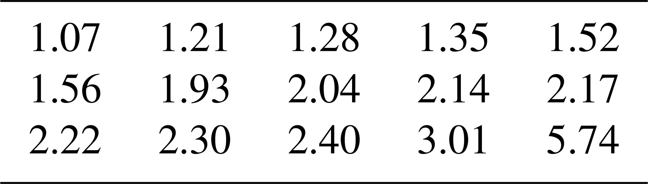
Subsequently, the 15 value that follows the cdf given in Eq. (9) with parameter b=1 and q=0.5 with t=1 are listed in increasing order in the Table 1.

Table 1 The 15 Data generated which follows the q-PD for q=0.5 and b=1 with t=1.

Source: Laboratory of Applied Mathematics, Mohamed Khider University, Biskra, Algeria.

First, we note that C_i=X_i with t=1 for $\mathrm{1}\le i\le \mathrm{15}$ and we get the range $A=\left\{b>\mathrm{0},\mathrm{0}<q<\mathrm{1};\mathrm{1}<X_i<e^{\mathrm{2}}\right\}$ for q=0.5 with b=1. And from the Table 1 we find $min\left(X_i\right)=\mathrm{1.07}>\mathrm{1}$ and $max\left(X_i\right)=\mathrm{5.74}<\exp \left(\mathrm{2}\right)$ this shows that for $i=\mathrm{1},\mathrm{\dots },n$ all sample values X_i in the Table 1 are belong to the set A.

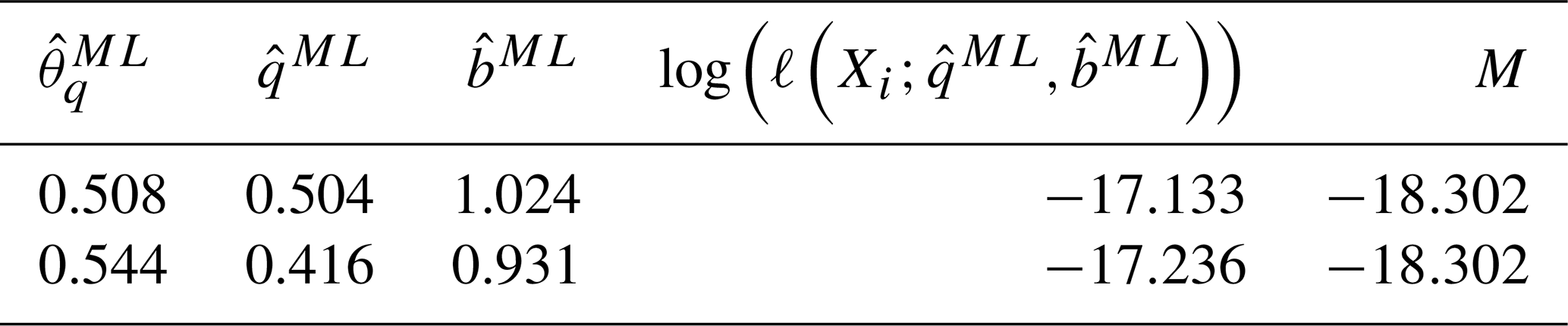
Next, compute the bounds given by ${\mathit{\theta }}_q^L=-\mathrm{3.01}\times {\mathrm{10}}^{\mathrm{2}}$ and $\mathit{ϵ}=-\mathrm{1.51}\times {\mathrm{10}}^{-\mathrm{7}}$ with ${\mathit{\theta }}_q^U=\mathrm{5.72}\times {\mathrm{10}}^{-\mathrm{1}}$ for search the roots of ψ(θ_q)=0 which is given in Eq. (30) via the MBA for multi-roots on the intervals $\left[{\mathit{\theta }}_q^L,-\mathit{ϵ}\right]$ and $\left[\mathit{ϵ},{\mathit{\theta }}_q^U\right]$. Then we find tow zero's ${\left({\mathit{\theta }}_q\right)}_{\mathrm{1}}^{\left(\mathrm{0}\right)}=\mathrm{0.508}$ or ${\left({\mathit{\theta }}_q\right)}_{\mathrm{2}}^{\left(\mathrm{0}\right)}=\mathrm{0.544}$. Next, Using formulas (33), (34) and (19), (25) to determine the values for each value ${\widehat{\mathit{\theta }}}_q^{ML}$ which are ${\widehat{q}}^{ML}$, ${\widehat{b}}^{ML}$ and $\log \left(\mathrm{\ell }\left(X_i;{\widehat{q}}^{ML},{\widehat{b}}^{ML}\right)\right)$, M respectively. The following Table 2 shows these results.

Table 2 An account the values corresponding to each value of ${\widehat{\mathit{\theta }}}_q^{ML}$.

Source: Laboratory of Higher School of Social Security, Mohamed saleh Mentouri, Ben Aknoûn, Algiers, Algeria.

Obviously, from Table 2 that for every ${\widehat{\mathit{\theta }}}_q^{ML}$ we find that ${\widehat{q}}^{ML}\in A$ and ${\widehat{b}}^{ML}\in A$ are the local maximum log-likelihood of the q-PD on A with $\log \left(\mathrm{\ell }\left(X_i;{\widehat{q}}^{ML},{\widehat{b}}^{ML}\right)\right)>M$. Wherever, the boundary maximum with $\widehat{q}=\mathrm{0}$ or $\widehat{q}=\mathrm{1}$ and $\widehat{b}=\mathrm{0.572}$ is given as $\log \left(\mathrm{\ell }\left(X_i;\mathrm{0},\mathrm{0.572}\right)\right)=\log \left(\mathrm{\ell }\left(X_i;\mathrm{1},\mathrm{0.572}\right)\right):=\mathrm{18.302}$ for $\widehat{b}$ in Eq. (25). And referring to the table we will find that maximum $\log \left(\mathrm{\ell }\left(X_i;{\widehat{q}}^{ML},{\widehat{b}}^{ML}\right)\right)$ is with ${\widehat{q}}^{ML}=\mathrm{0.504}$ and ${\widehat{b}}^{ML}=\mathrm{1.024}$. Then the q-PD maximum likelihood estimates for the data given in Table 1 are ${\widehat{q}}^{ML}=\mathrm{0.504}$ and ${\widehat{b}}^{ML}=\mathrm{1.024}$. It is clear that $\left({\widehat{q}}^{ML},{\widehat{b}}^{ML}\right)$ is very close to the values that we proposed to conduct the simulation. Then, their corresponding 95 % confidence intervals are $\mathrm{0.03912}<q<\mathrm{0.96888}$ and $\mathrm{0.3685}<b<\mathrm{1.6795}$.

3.2 Application

Earthquake magnitude scales measure the total energy released from the earthquake's epicenter. These scales use a logarithmic scale, where each incremental increase represents an exponential jump in both amplitude and energy. The Richter scale, developed in 1935, is an older scale that measures the maximum amplitude of seismic waves on a seismograph. This scale is accurate for small to moderate local earthquakes but becomes less accurate for large earthquakes. However, because magnitude scales are logarithmic, the energy jump between increments is enormous. With each incremental increase, the amplitude of the vibration increases approximately 10-fold, and the actual energy released increases approximately 32-fold.

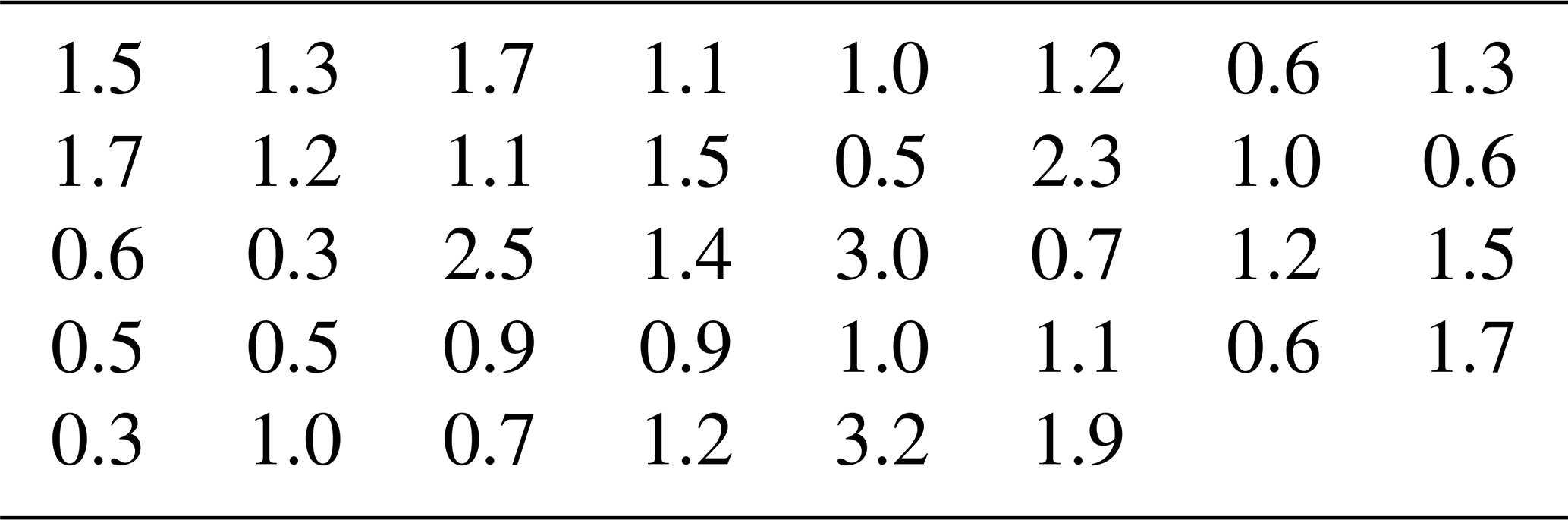
Carefully, this represents a list that contains information about the tectonic earthquake activity (magnitudes) in and around the British Isles in the last 60 d from 22 March to 20 May 2024. We find that the 38 value (C₁, C₂, …, C₃₈) of the exceedance of the threshold (The known value of the earthquake intensity threshold is not mentioned for reasons related to intellectual property rights) in the tectonic earthquake activity is shown in the following Table 3.

Table 3 Earthquakes occurred around the British Isles from 22 March to 20 May 2024.

Note: The data are from the following link https://earthquakes.bgs.ac.uk/earthquakes/recent_uk_events.html (last access: May 2024).

We know that the earthquake activity data are always positive values and that they follow a q-PD parameter (9). We take the value 38 in the Table 3 as $\left(\log X_{\mathrm{1}},\mathrm{\dots },\log X_{\mathrm{38}}\right)$, therefore, we agree that the threshold $t<min\left(X_i\right)=\mathrm{1}$ for $i=\mathrm{1},\mathrm{\dots },\mathrm{38}$ because the data $\left(\log X_{\mathrm{1}},\mathrm{\dots },\log X_{\mathrm{38}}\right)$ are absolutely positive values. After applying the algorithm (Sect. 2.1) to the sample in the Table 3 we find that the q-PD maximum likelihood estimates are ${\widehat{q}}^{ML}=\mathrm{0.4769504}$ and ${\widehat{b}}^{ML}=\mathrm{0.5569276}$ with corresponding 95 % confidence intervals are $\mathrm{0.2107213}<q<\mathrm{0.7431795}$ and $\mathrm{0.3453592}<b<\mathrm{0.7684960}$.

4 Conclusions

In this work, we focus on estimating the parameters of q-PD (Eq. 9) by presenting an algorithm (Sect. 2.1) based on the MLE method and we have obtained results that we will mention. In addition, we give a new formulation of the distribution of the G-ED which is given in Eq. (6). Since we linked the GPD parameters (Eq. 12) and the G-ED (Eq. 6) using the relationship (16), we managed to approximate the distribution function of exceedances over a threshold that is given in Eq. (15) to the G-ED under the Theorem 1. In addition, we can estimate the index of the extreme value by estimating the shape parameter of the G-ED with the MLE method using the relation (16). Therefore, we find that this work will provide a foundation for other work related to the results we achieved in this article.

Appendix A: The second-order derivatives of the log-likelihood for the q-PD

The second-order derivatives of the log-likelihood of the q-PD which defined in Eq. (19) are calculating by

$$\left\{\begin{array}{l}\frac{{\partial }^{\mathrm{2}}\log \left(\mathrm{\ell }\left(C_i;q,b\right)\right)}{{\partial }^{\mathrm{2}}q}=\frac{\mathrm{1}}{{\left(q-\mathrm{1}\right)}^{\mathrm{3}}}\sum _{i=\mathrm{1}}^n[q\log {\left(\mathrm{1}-\frac{\mathrm{1}}{\mathit{\phi }\left(C_i\right)}\right)}^{\mathrm{2}}\\ -\mathrm{2}\log \left(\mathit{\phi }\left(C_i\right)\right)+\mathrm{2}\left(\mathrm{1}-\frac{\mathrm{1}}{\mathit{\phi }\left(C_i\right)}\right)]\\ \frac{{\partial }^{\mathrm{2}}\log \left(\mathrm{\ell }\left(C_i;q,b\right)\right)}{{\partial }^{\mathrm{2}}b}={\left(\frac{q-\mathrm{1}}{{\mathit{\theta }}_q}\right)}^{\mathrm{2}}\sum _{i=\mathrm{1}}^n\left[\frac{q}{q-\mathrm{1}}{\left(\mathrm{1}-\frac{\mathrm{1}}{\mathit{\phi }\left(C_i\right)}\right)}^{\mathrm{2}}-\mathrm{1}\right]\\ \frac{{\partial }^{\mathrm{2}}\log \left(\mathrm{\ell }\left(C_i;q,b\right)\right)}{\partial q\partial b}=\frac{\mathrm{1}}{{\mathit{\theta }}_q}\sum _{i=\mathrm{1}}^n\left[\left(\mathrm{1}-\frac{\mathrm{1}}{\mathit{\phi }\left(C_i\right)}\right)-\frac{q}{q-\mathrm{1}}{\left(\mathrm{1}-\frac{\mathrm{1}}{\mathit{\phi }\left(C_i\right)}\right)}^{\mathrm{2}}\right]\end{array}\right.$$

where ${\mathit{\theta }}_q=-\left(q-\mathrm{1}\right)b$ and $\mathit{\phi }\left(x\right)=\mathrm{1}-{\mathit{\theta }}_q\log \left(x\right)$ with $C_i=\frac{X_i}{t}$ for X_i>t and t>0.