Comparative evaluation of statistical and deep learning methods for high-frequency radar surface current forecasting in a narrow tropical strait

Accurate prediction of ocean surface currents is essential for maritime safety in narrow waterways with strong tidal forcing. This study presents a three-phase evaluation of forecasting methods for high-frequency (HF) radar surface currents in the Sunda Strait, Indonesia, where tidal currents regularly exceed 150 cm s⁻¹. Phase 1 compares twelve methods – persistence, tidal harmonics, classical time series, a reduced-rank spatio-temporal statistical model, shallow machine learning, and deep learning – for one-step-ahead prediction; evaluated consistently over all 291 grid cells and the full test period, the deep learning models achieve the lowest root-mean-square errors (RMSE) for both components, with the convolutional neural network (CNN) reaching 11.31 cm s⁻¹ for the zonal component (skill score 0.50 relative to persistence) and the convolutional neural network–gated recurrent unit (CNN-GRU) reaching 15.44 cm s⁻¹ for the meridional component (skill score 0.42); the pointwise classical statistical models (autoregressive integrated moving average, ARIMA; exponential smoothing) fall well below, while an empirical-orthogonal-function vector autoregression (EOF-VAR) that models spatial correlation closes most of the gap to deep learning, indicating that the neglect of spatial structure – not of nonlinearity – is the principal limitation of the classical baselines. Phase 2 examines lookback window length (T = 3, 6, 12 h); CNN-gated recurrent unit (CNN-GRU) improves monotonically with longer lookback, reaching 11.21 and 15.41 cm s⁻¹ at T = 12, while standalone CNN and GRU show no benefit. Phase 3 extends prediction to six-hour nowcasting using direct multi-step and autoregressive (ConvLSTM-ED, BiEF) architectures; under a controlled comparison (five seeds, identical training budget on one GPU), accuracy is governed by model capacity and plateaus near 1 M parameters (the 1.00 M CNN-GRU-MS-Small reaching 18.39 and 22.07 cm s⁻¹; skill scores 0.77 and 0.72), and at matched capacity the direct and autoregressive architectures are statistically indistinguishable. The direct multi-step model is nonetheless preferred for operational nowcasting because it trains ∼2.5 times faster and runs ∼4.5 times faster at inference (a single forward pass versus sequential decoding). Diurnal error analysis, corroborated by concurrent wind observations from three coastal weather stations, reveals that zonal prediction errors correlate positively with afternoon sea-breeze wind enhancement (Spearman r_s = 0.48 across the 24 diurnal-mean hours), while meridional errors follow a distinct diurnal pattern not explained by wind forcing. Relative errors of 3 %–7 % of the observed speed range are of the same order as those reported in calmer environments – though this normalisation partly reflects the strait's very large speed range – suggesting that deep learning does not break down in energetic strait settings.

1 Introduction

The prediction of ocean surface currents is a fundamental challenge in operational oceanography, with applications spanning maritime navigation, search-and-rescue operations, oil spill trajectory forecasting, and coastal environmental management (Allard et al., 2014). In narrow strait environments, where tidal amplification can produce surface currents exceeding 150 cm s⁻¹ (Susanto et al., 2016), accurate short-term forecasts are especially critical for shipping safety and port operations.

High-frequency (HF) radar provides spatially continuous, real-time surface current measurements at hourly or sub-hourly temporal resolution (Paduan and Washburn, 2013; Roarty et al., 2024). The resulting spatiotemporal data present a natural prediction problem: given the observed current field over a lookback window of T timesteps, forecast the field one or more steps ahead. This problem admits solutions from a hierarchy of statistical and computational methods, ranging from simple persistence and autoregressive models to deep neural networks designed for spatiotemporal sequence prediction.

Several studies have applied deep learning to HF radar current prediction. Thongniran et al. (2019b) introduced a CNN-GRU architecture combining convolutional neural networks (CNN) for spatial feature extraction with gated recurrent units (GRU; Cho et al., 2014) for temporal modelling, reporting RMSE improvements of 11 % and 27 % over standalone models in the Gulf of Thailand. Follow-up work incorporated attention mechanisms (Thongniran et al., 2019a), and Chen and Chi (2021) proposed a spatiotemporal attention-based GRU. For multi-step forecasting, convolutional long short-term memory (ConvLSTM) encoder–decoder architectures (Shi et al., 2015), which extend the long short-term memory cell (Hochreiter and Schmidhuber, 1997) with convolutional state transitions, have been applied to sea surface temperature prediction (Xiao et al., 2019; Zhang et al., 2020; Wei and Guan, 2022) and four-dimensional ocean temperature forecasting (Liu et al., 2024), but their application to surface current nowcasting remains limited. Zhang and Yin (2024) demonstrated a residual-learning CNN with attention for offshore current field forecasting, and Zhang et al. (2024) presented a physics-informed model for surface current prediction. Earlier neural network approaches include Kalinić et al. (2017) and Ren et al. (2018), who applied feedforward and recurrent networks to coastal currents. Recent advances include deep learning for ocean current estimation from satellite altimetry and sea surface temperature (Ciani et al., 2025) and end-to-end neural global ocean forecasting (El Aouni et al., 2025). Reviews by Dong et al. (2022) and Zhao et al. (2024) document the growing role of deep learning in physical oceanography.

Despite these advances, several gaps remain. First, most studies have been conducted in open-sea environments where current speeds are moderate (typically below 50 cm s⁻¹); performance in energetic strait environments has not been systematically evaluated. Second, the relationship between lookback window length and prediction skill – particularly the role of tidal cycle coverage – has not been explicitly investigated. Third, the transition from one-step to multi-step prediction introduces a design choice between autoregressive and direct prediction strategies, the trade-offs of which have not been studied for HF radar currents in tidally dominated settings.

This study addresses these gaps through a three-phase evaluation using over three years of hourly HF radar data from the Sunda Strait, Indonesia:

1. Phase 1 compares twelve forecasting methods for one-step-ahead prediction, including UTide tidal harmonic predictions and a reduced-rank spatio-temporal statistical model (EOF-VAR) alongside persistence;

2. Phase 2 examines the sensitivity of the three best deep learning architectures to lookback window length (T = 3, 6, 12 h);

3. Phase 3 extends prediction to six-hour nowcasting using ConvLSTM encoder–decoder (ConvLSTM-ED), bidirectional ConvLSTM encoder–forecaster (BiEF), and direct multi-step CNN-GRU (CNN-GRU-MS).

The main contributions are: (i) a comprehensive benchmark spanning persistence, classical and spatio-temporal statistical models, and deep learning (twelve methods) for HF radar currents in a narrow tropical strait with strong tidal forcing; (ii) demonstration that tidal cycle coverage in the lookback window is the primary driver of skill improvement for hybrid architectures; (iii) a controlled multi-seed, capacity-matched comparison showing that direct and autoregressive multi-step architectures achieve comparable accuracy, with the direct model preferred operationally for its $\sim \mathrm{2.5}\times$ faster training and $\sim \mathrm{4.5}\times$ faster single-pass inference; and (iv) diurnal and seasonal error analysis linked to concurrent meteorological observations.

2 Study area and data

2.1 The Sunda Strait

The Sunda Strait connects the Java Sea to the Indian Ocean between the islands of Java and Sumatra, Indonesia (Fig. 1). The strait is approximately 24 km wide at its narrowest point and experiences strong tidal forcing dominated by the semidiurnal M2 constituent (∼12.42 h period). Surface currents regularly exceed 150 cm s⁻¹ (Susanto et al., 2016). The circulation is modulated by two monsoon seasons: the northwest (NW) monsoon (December–February) and the southeast (SE) monsoon (June–August) (Wyrtki, 1961; Li et al., 2018). The strait serves as a secondary pathway for the Indonesian Throughflow (ITF) (Sprintall et al., 2019). Mujiasih et al. (2021) previously demonstrated the value of HF radar observations in this region.

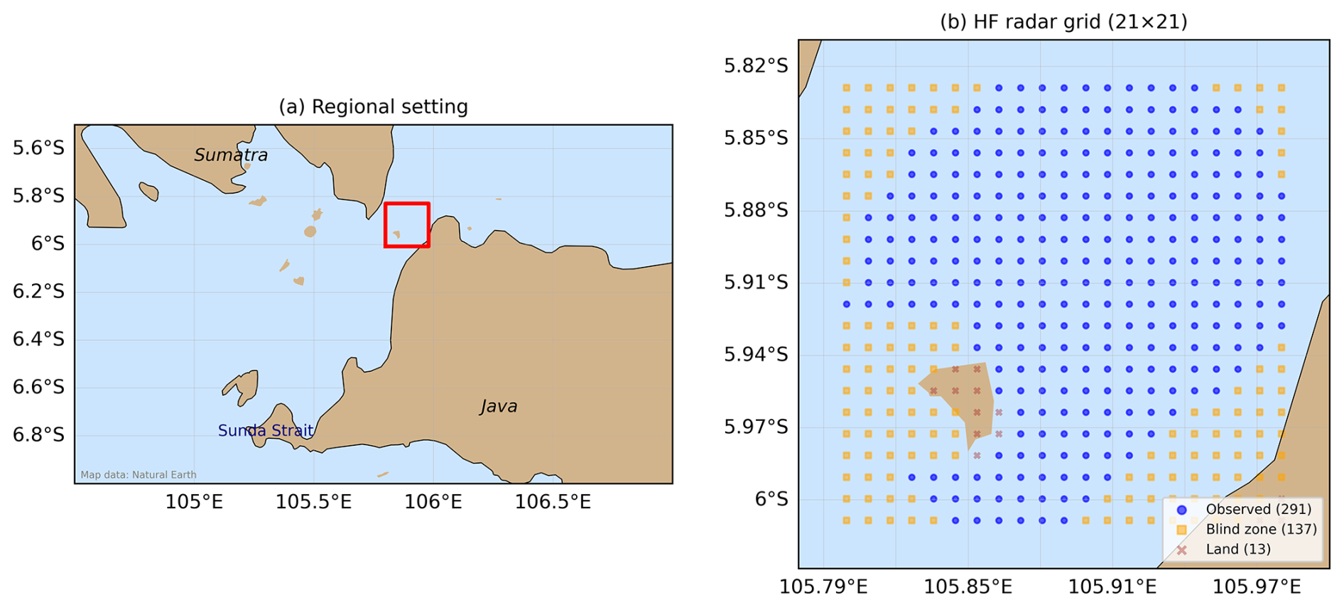
Figure 1 (a) Regional map showing the Sunda Strait between Java and Sumatra, Indonesia (map data: Natural Earth). (b) HF radar grid (21×21) showing 291 observed sea points (blue), 137 blind-zone sea points (orange), and 13 land points (brown) at approximately 1 km spacing.

2.2 HF radar observations and quality control

The BADA (Bidirectional Array Direction of Arrival) HF radar system, a Coastal Ocean Dynamics Applications Radar (CODAR) type direction-finding radar operating at 13.5 MHz, is operated by the Indonesia Meteorology, Climatology, and Geophysical Agency (BMKG). It provides hourly measurements of the eastward (zonal, U) and northward (meridional, V) surface current components across 291 active grid points on a 21×21 spatial grid (∼1 km resolution). The dataset spans December 2022–February 2026, providing 28 321 hourly timesteps.

Quality control follows established HF radar protocols (He et al., 2023; Roarty et al., 2024): (1) speed thresholding at 200 cm s⁻¹, (2) temporal consistency checks requiring less than 100 cm s⁻¹ change between consecutive hours, and (3) spatial median absolute deviation (MAD) filtering with a factor of three. After quality control, temporal coverage is approximately 85 %. Missing values at each grid point are filled using tidal harmonic predictions from UTide (Codiga, 2011) fitted to the available record at that point, ensuring gap-free lookback windows for all models.

The data are split chronologically: training (December 2022–December 2024; 18 216 steps), validation (January–June 2025; 4344 steps), and test (July 2025–February 2026; 5761 steps). The training set spans approximately two years, covering at least three complete monsoon seasons (SE 2023, NW 2023/24, SE 2024) and portions of the NW monsoon at both ends of the period.

For diurnal error analysis, concurrent wind observations are obtained from three BMKG automatic weather stations (AWS) at Merak, Ciwandan, and Bakauheni ports surrounding the Sunda Strait, providing 1 min wind speed and direction over January 2025–April 2026, of which the July 2025–February 2026 test period is used for the diurnal error analysis. These are averaged to hourly resolution with basic quality control (removal of wind speeds exceeding 40 m s⁻¹).

3 Methods

3.1 Problem formulation

The prediction task is formulated at two levels. For one-step prediction (Phases 1–2), given the observed current field over a lookback window of T timesteps, the goal is to predict the field at t+1:

$$\begin{array}{}\text{(1)}& \widehat{\mathbf{X}}(t+\mathrm{1})=f\left(\mathbf{X}\right(t),\mathbf{X}(t-\mathrm{1}),\mathrm{\dots },\mathbf{X}(t-T+\mathrm{1}\left)\right)\end{array}$$

where $\mathbf{X}\left(t\right)\in {\mathbb{R}}^{\mathrm{2}\times \mathrm{21}\times \mathrm{21}}$ contains the U and V fields at time t. Of the $\mathrm{21}\times \mathrm{21}=\mathrm{441}$ grid cells, 291 are observed sea points, 137 are coastal blind-zone sea points (outside the radar footprint), and 13 are land; blind-zone and land cells are set to zero in the input and excluded from the loss function and evaluation metrics.

For multi-step nowcasting (Phase 3), the prediction extends over a horizon H = 6 h:

$$\begin{array}{}\text{(2)}& \left[\widehat{\mathbf{X}}\right(t+\mathrm{1}),\mathrm{\dots },\widehat{\mathbf{X}}(t+H\left)\right]=g\left(\mathbf{X}\right(t),\mathrm{\dots },\mathbf{X}(t-T+\mathrm{1}\left)\right)\end{array}$$

The neural-network inputs and targets are normalised to [0,1] using min–max scaling computed on the training set only; the training-set extremes are $U\in [-\mathrm{185.4},\mathrm{153.3}]$ cm s⁻¹ and $V\in [-\mathrm{197.3},\mathrm{196.4}]$ cm s⁻¹. This [0,1] scaling is applied only to the neural networks: the classical statistical baselines (UTide, moving average, exponential smoothing, and ARIMA) and the EOF-VAR model are fitted directly to the raw current series in cm s⁻¹ (Sect. 3), so the ARIMA error model in particular operates on the unbounded real line rather than on bounded [0,1] data. All neural networks use mean squared error (MSE) over the 291 observed sea cells as the loss function and default PyTorch weight initialisation (Kaiming uniform for convolutional layers, uniform for linear and recurrent layers).

3.2 Phase 1: one-step prediction methods

Twelve methods are compared, spanning six categories (Table 1). All methods use a default lookback of T = 3. The methods were chosen to span the full ladder relevant to operational HF-radar nowcasting – a naive persistence reference, a deterministic-physical baseline (tidal harmonics), classical univariate time-series models, a reduced-rank spatio-temporal statistical model that accounts for spatial correlation (EOF-VAR), shallow machine learning, and spatio-temporal deep learning – and to include the specific architectures previously applied to HF-radar currents (CNN-GRU; ConvLSTM, Phase 3) so that our energetic-strait results are directly comparable to earlier open-sea studies. Approaches deliberately left for future work include attention/transformer sequence models and graph neural networks.

Table 1 Summary of all forecasting methods evaluated in this study, grouped by category and phase.

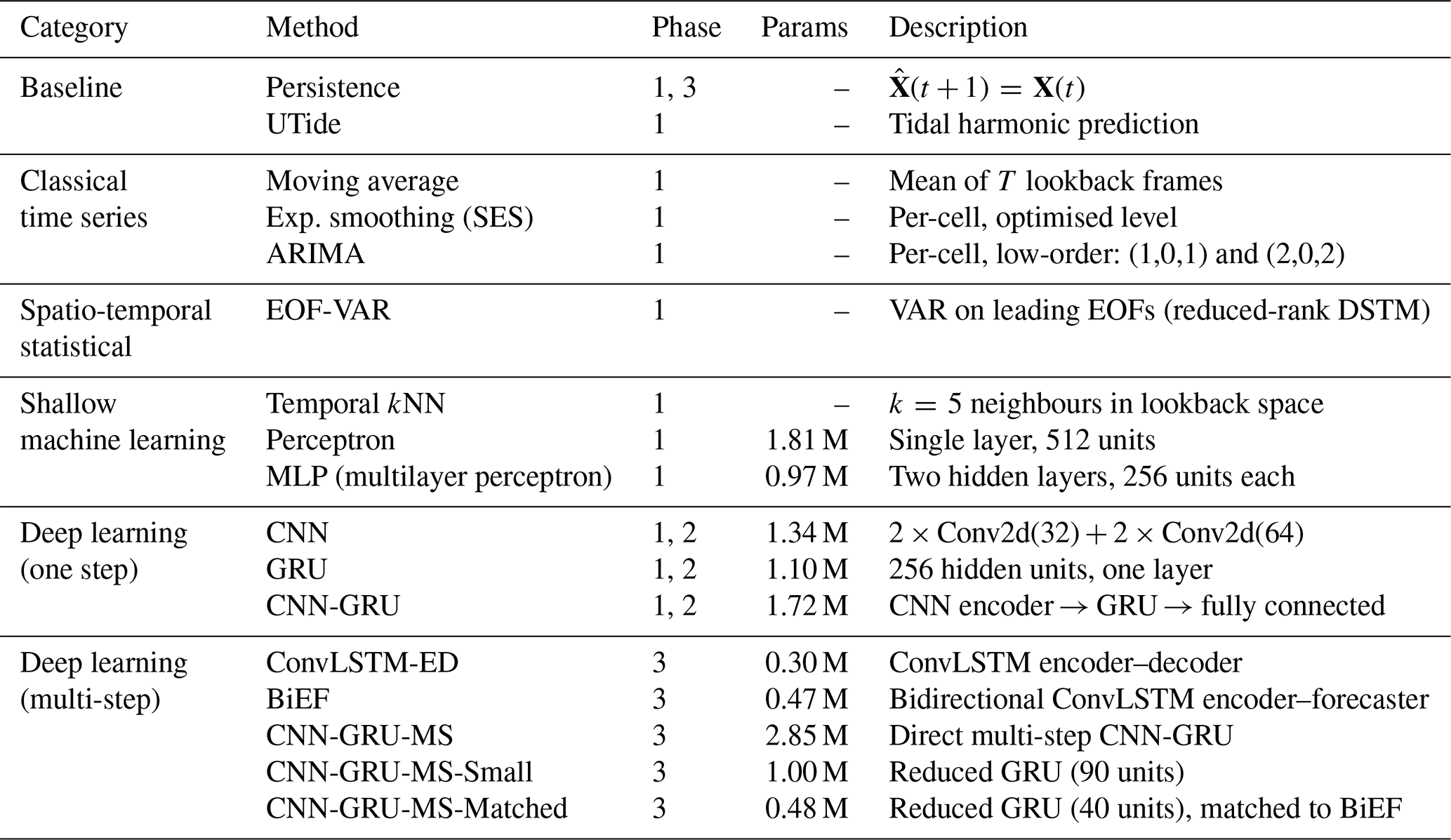
The persistence model predicts the most recent observation: $\widehat{\mathbf{X}}(t+\mathrm{1})=\mathbf{X}\left(t\right)$. The UTide baseline predicts using tidal harmonic analysis (Codiga, 2011) fitted independently at each grid point using eight major constituents (M2, S2, K1, O1, N2, K2, P1, M4), representing the deterministic tidal component. The moving average predicts the mean of the T lookback frames, effectively a low-pass filter that smooths both signal and noise. Simple exponential smoothing (SES) forecasts the next value as an exponentially weighted average of the past, with the smoothing level optimised per cell on the training set. ARIMA (Box et al., 2015) is fitted independently to each grid cell on the raw current series (cm s⁻¹); only the neural networks use the [0,1] min–max scaling, so the ARIMA error model operates on the unbounded real line. Because min–max scaling is an invertible affine transform under which ARIMA is equivariant, this choice does not affect the reported errors – it only keeps the Gaussian error model on the natural unbounded scale. The AR term captures the strong one-step autocorrelation of tidal currents and the MA term smooths observation noise. No differencing (d = 0) is applied: augmented Dickey–Fuller tests reject the unit root in all 30 cells of a representative sample for both components (median $p=\mathrm{2.4}\times {\mathrm{10}}^{-\mathrm{5}}$ for U, $\mathrm{7.0}\times {\mathrm{10}}^{-\mathrm{7}}$ for V), confirming stationarity. The sample autocorrelation and partial-autocorrelation functions (Fig. 2) show the strongly oscillatory structure of a deterministic semidiurnal tide – not the rapidly decaying signature of an autocorrelated-noise process – with significant partial autocorrelations extending to lags well beyond those an ARMA(1,1) can represent. Evaluating AIC across low orders $(p,d,q)\in \mathit{\{}\mathrm{0},\mathrm{1},\mathrm{2}{\mathit{\}}}^{\mathrm{2}}\times \mathit{\{}\mathrm{0},\mathrm{1}\mathit{\}}$ favours (2,0,2) in 54 of 60 cell-series. Because this optimum lies on the boundary of the search set, we extended the search to $p,q\le \mathrm{4}$ (d = 0): the AIC optimum then moves beyond the original boundary in all 60 cell-series – most frequently (3,0,4) (28 series) and (4,0,4) (14 series), again often on the boundary of the extended set – and adding a seasonal component at the 12 h semidiurnal period reduces the AIC further in all 20 series tested. This boundary behaviour confirms that no finite low-order ARMA representation is adequate for these series, consistent with the quasi-deterministic tidal harmonics visible in Fig. 2, and the selected order varies from cell to cell, so no single higher order would be defensible as a uniform specification. Crucially, however, the higher-order and seasonal specifications do not materially improve out-of-sample forecasts: evaluated over the full 5761-step test period on the same cell sample, the per-series AIC-best orders ($p,q\le \mathrm{4}$) reduce the one-step RMSE relative to (2,0,2) by a median of only 0.29 cm s⁻¹ (≈2 %) while the mean change is a slight degradation of 0.18 cm s⁻¹ (individual cells improve or degrade), and the best seasonal specification improves the mean RMSE by only ∼0.6 cm s⁻¹ (≈4 %). We therefore retain ARIMA as an intentionally low-order empirical baseline: it is a data-driven model that encodes no tidal physics (the deterministic tidal prior is instead carried by the UTide baseline), and it is not expected to capture the underlying physical process in full. We report both the parsimonious ARIMA(1,0,1) and the low-order AIC-optimal ARIMA(2,0,2), and the comparison with the spatio-temporal models should be read with this qualification in mind. Ljung–Box tests show that residuals retain significant autocorrelation at all orders examined, including the seasonal specifications (p≈0 in essentially all cells; excess kurtosis ≈6, so the Gaussian likelihood acts as a quasi-maximum-likelihood estimator of the conditional mean), reflecting tidal harmonic structure that a per-cell low-order ARMA cannot fully capture. ARIMA, SES, and temporal kNN are evaluated on all 291 sea cells over the full test period; fitting ARIMA at all 291 cells is computationally inexpensive (about 17 min in total, far less than the time required to train the neural networks). The temporal kNN (Jirakittayakorn et al., 2017) (k = 5) fits a per-cell k-nearest-neighbours regressor on the lookback feature vector (Euclidean distance) and predicts the mean of the five nearest neighbours. As per-cell univariate models, the moving average, SES, ARIMA, and kNN have no spatial coupling and are therefore confined to Phase 1; the lookback-sensitivity (Phase 2) and multi-step spatio-temporal (Phase 3) experiments concern the joint spatial–temporal modelling these methods cannot perform.

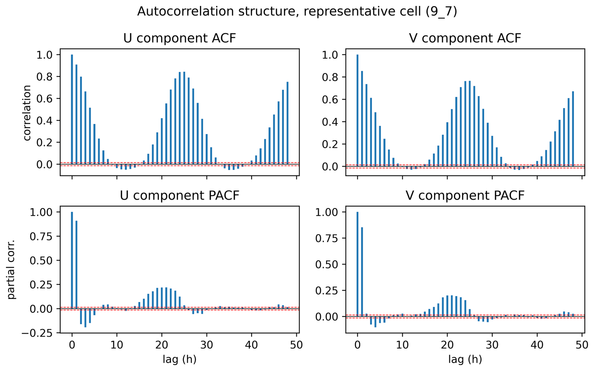
Figure 2 Sample autocorrelation (ACF) and partial autocorrelation (PACF) of the training-period U and V series at a representative cell. The oscillatory ACF reflects the deterministic semidiurnal tide; the PACF retains significant terms to lags far beyond the reach of an ARMA(1,1), explaining why AIC pushes the selected order to the boundary of the search set and why ARIMA residuals remain autocorrelated at all orders examined. Red dashed lines mark the $\pm \mathrm{1.96}/\sqrt{n}$ significance band.

To provide a statistical model that does account for spatial correlation – bridging the pointwise time-series methods and the spatio-temporal neural networks – we include an empirical-orthogonal-function vector autoregression (EOF-VAR), a standard reduced-rank dynamic spatio-temporal model (Cressie and Wikle, 2011; Wikle et al., 2019). The combined (U,V) field over the 291 sea cells is centred on the training mean and decomposed by truncated singular-value decomposition into empirical orthogonal functions (EOFs); the leading K = 11 modes capture 95 % of the training variance. A vector autoregression of order p (selected by AIC, giving p = 6) is fitted to the K principal-component time series, jointly modelling the temporal evolution of the dominant spatial modes. One-step-ahead forecasts of the principal components are reconstructed to the full field and scored identically to the other methods. EOF-VAR thus captures spatial covariance (through the shared EOFs) and temporal dynamics (through the VAR) within a linear statistical framework.

The perceptron is a single hidden layer of 512 units with rectified linear unit (ReLU) activation, taking the flattened lookback ($T\times \mathrm{2}\times \mathrm{21}\times \mathrm{21}=\mathrm{2646}$ features) as input. The MLP uses two hidden layers of 256 units each with ReLU activation. Both use a sigmoid output layer to predict the normalised [0,1] current field.

The CNN (LeCun et al., 1998) uses two blocks of Conv2d layers (32 and 64 filters, 3×3 kernels, exponential linear unit (ELU) activation) with 2×2 max-pooling and dropout (0.2) after each block. All T lookback frames are stacked along the channel dimension ($T\times \mathrm{2}=\mathrm{6}$ input channels for T = 3). The feature maps are flattened and passed through a fully connected layer of 512 units (ReLU) followed by a sigmoid output layer. Figure 3 illustrates the CNN architecture.

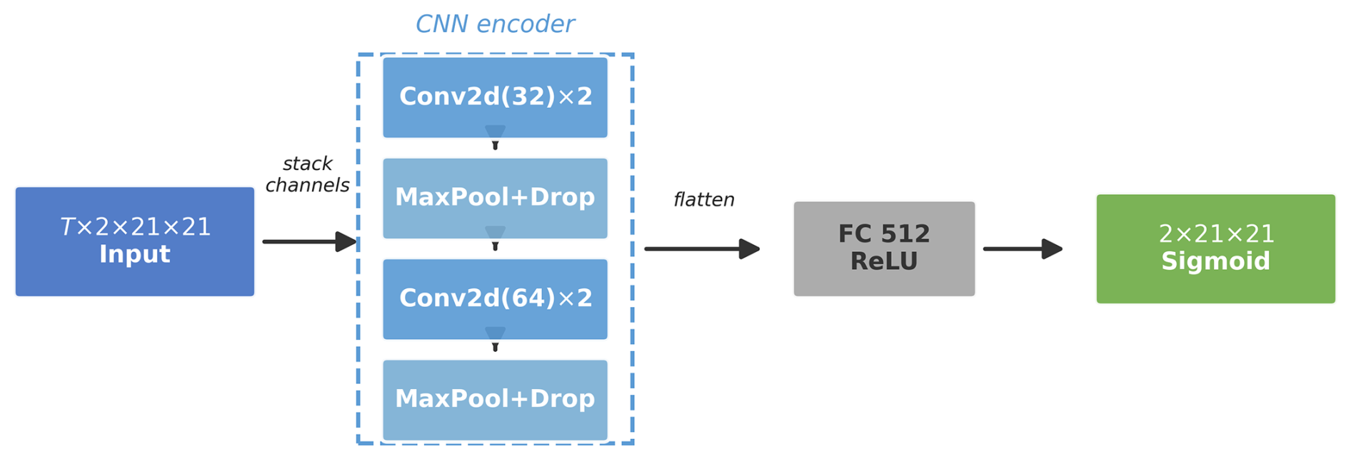
Figure 3 CNN architecture. All T lookback frames are stacked along the channel dimension and processed by two convolutional blocks (32 and 64 filters), followed by flattening and a fully connected output layer (1.34 M parameters).

The GRU (Cho et al., 2014) processes the flattened frame sequence through a 256-unit recurrent layer; at each timestep, the $\mathrm{2}\times \mathrm{21}\times \mathrm{21}=\mathrm{882}$ values are flattened into a single vector, and the final hidden state is decoded via a fully connected layer with sigmoid activation. Figure 4 illustrates the GRU architecture.

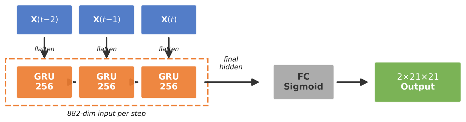
Figure 4 GRU architecture. Each lookback frame is flattened to an 882-dimensional vector and fed sequentially to a 256-unit GRU layer. The final hidden state is decoded via a fully connected layer (1.10 M parameters).

The CNN-GRU (Thongniran et al., 2019b) applies the CNN encoder independently to each lookback frame, extracting a spatial feature vector per timestep. The resulting feature sequence is passed to the GRU, and the final hidden state is decoded via a fully connected output layer with sigmoid activation. Figure 5 illustrates the CNN-GRU architecture.

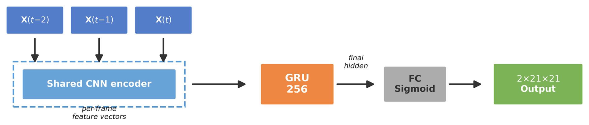
Figure 5 CNN-GRU architecture. A shared CNN encoder extracts spatial features from each lookback frame independently; the resulting feature sequence is processed by the GRU, and the final hidden state is decoded to the output field (1.72 M parameters).

All neural networks are trained with Adam (Kingma and Ba, 2015) (lr $={\mathrm{10}}^{-\mathrm{3}}$), early stopping (patience 10), batch size 64, and a maximum of 50 epochs.

3.3 Phase 2: lookback sensitivity

Phase 2 carries forward the three deep learning models from Phase 1 (CNN, GRU, CNN-GRU), defined as the architectures attaining the lowest Phase 1 validation RMSE among the spatio-temporal candidates. The per-cell statistical methods (moving average, SES, ARIMA, kNN) are univariate and have no lookback-window analogue, so they are confined to Phase 1 (Sect. 3); ARIMA in particular is not carried forward because it is a per-cell model incompatible with the joint spatio-temporal task – and, on the full-domain evaluation, it is not the best method for V in any case (Sect. 4). The three deep learning models are retrained with lookback windows of T = 3, 6, and 12 h. At T = 12 h, the lookback approximately covers one full semidiurnal M2 tidal cycle, providing complete tidal phase information.

3.4 Phase 3: multi-step nowcasting architectures

Phase 3 addresses a different task – six-hour multi-step nowcasting rather than one-step prediction – which requires architectures that emit a full H-step forecast. We therefore introduce three multi-step architectures rather than reusing the Phase 1 one-step models directly; the design builds on the Phase-1/2 finding that the CNN-GRU hybrid is the strongest one-step spatio-temporal model, which motivates the direct multi-step CNN-GRU-MS evaluated here against two autoregressive ConvLSTM baselines. Three architectures are compared for six-hour nowcasting, all using T = 12:

The ConvLSTM encoder–decoder (ConvLSTM-ED) uses a single ConvLSTM layer (Shi et al., 2015) with 64 hidden channels and 3×3 kernels to encode the T-step input. The decoder is another ConvLSTM layer that autoregressively generates H output frames, each conditioned on the previous prediction. A 1×1 convolution maps hidden states to the two-channel (U, V) output at each step (305 K parameters). Figure 6 illustrates the ConvLSTM-ED architecture.

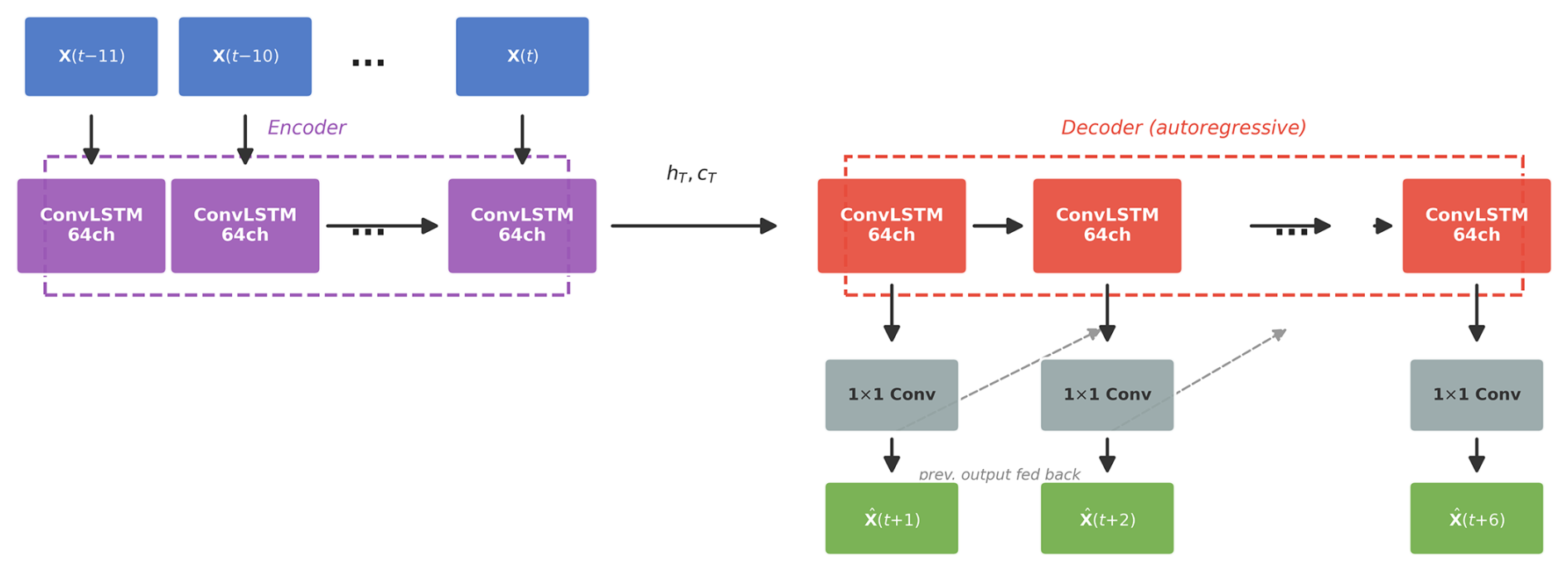
Figure 6 ConvLSTM-ED architecture. The encoder processes T input frames through a ConvLSTM layer (64 hidden channels); the decoder autoregressively generates H output frames, each conditioned on the previous prediction via feedback (dashed arrows). A 1×1 convolution maps hidden states to the output at each step (305 K parameters).

The bidirectional encoder–forecaster (BiEF) extends the encoder with forward and backward ConvLSTM passes (Schuster and Paliwal, 1997). The forward and backward hidden and cell states are concatenated and merged via a shared 1×1 convolution (128→64 channels), and the decoder is identical to ConvLSTM-ED (465 K parameters). Figure 7 illustrates the BiEF architecture.

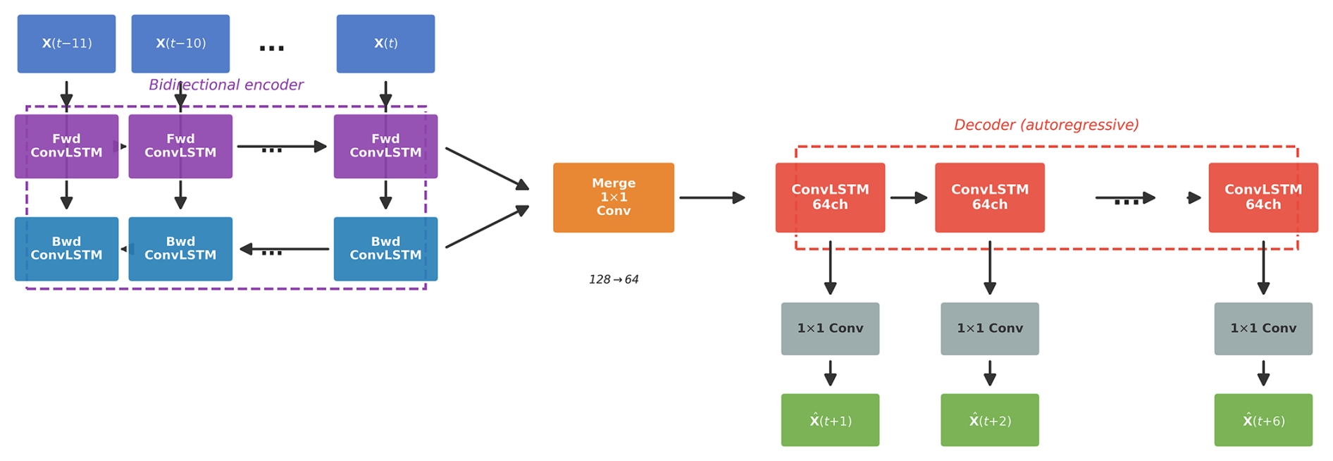
Figure 7 BiEF architecture. Bidirectional forward and backward ConvLSTM encoders process the input sequence in both directions; the resulting states are merged via a 1×1 convolution (128→64 channels) before the same autoregressive decoder as ConvLSTM-ED (465 K parameters).

The direct multi-step CNN-GRU (CNN-GRU-MS) extends the Phase 1 CNN-GRU to predict all H future frames simultaneously in a single forward pass, without autoregressive decoding. The GRU hidden state is mapped to $H\times \mathrm{2}\times \mathrm{21}\times \mathrm{21}$ via a fully connected layer with sigmoid activation (2.85 M parameters). Two reduced-capacity variants are also trained to assess the influence of model capacity on the comparison with the autoregressive models: CNN-GRU-MS-Small (GRU hidden size 90, 1.00 M parameters) and CNN-GRU-MS-Matched (GRU hidden size 40, 0.48 M parameters, capacity-matched to BiEF). Figure 8 illustrates the CNN-GRU-MS architecture.

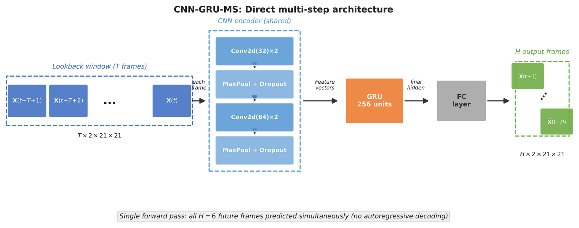
Figure 8 CNN-GRU-MS architecture. The shared CNN encoder extracts spatial features from each lookback frame independently; the GRU processes the resulting feature sequence; and a fully connected layer maps the final hidden state directly to all H = 6 future frames without autoregressive decoding (2.85 M parameters).

Phase 3 models are trained with Adam (lr = 10⁻³), early stopping (patience 5), batch size 32, maximum 20 epochs, and gradient clipping at 1.0 for all three architectures. The reduced batch size (32 vs. 64 in Phase 1) accommodates the larger memory footprint of multi-step sequences. The Phase-1 and Phase-2 models were trained on an Intel Core i7-12700 CPU with Intel Extension for PyTorch (IPEX); the controlled multi-step comparison in Tables 4 and 5 was run separately, retraining all five Phase-3 architectures over five seeds ($\mathit{\{}\mathrm{42},\mathrm{123},\mathrm{456},\mathrm{789},\mathrm{1024}\mathit{\}}$) under these identical settings on a single GPU (per-seed training and single-CPU inference times are reported in Table 5).

3.5 Evaluation metrics

The primary metric is root-mean-square error (RMSE) computed over all 291 sea grid points and test timesteps. Following Murphy (1988), the forecast skill score relative to persistence is defined using the MSE as

$$\begin{array}{}\text{(3)}& \text{SS}=\mathrm{1}-{\displaystyle \frac{{\text{MSE}}_{\text{model}}}{{\text{MSE}}_{\text{persistence}}}}\end{array}$$

where SS>0 indicates improvement and SS = 1 is a perfect forecast. For Phase 3, the step-k persistence ($\widehat{\mathbf{X}}(t+k)=\mathbf{X}\left(t\right)$) is used as the reference at each lead time.

Diurnal error patterns are assessed by stratifying per-timestep squared errors by hour of day. To quantify stochastic training variability, the three Phase 1 deep learning models and the Phase 3 CNN-GRU-MS are retrained with five random seeds (42, 123, 456, 789, 1024) each; mean and standard deviation of the RMSE are reported alongside single-run values. Following the philosophy of Diebold and Mariano (1995), we interpret model ranking primarily through effect sizes (RMSE differences) rather than p-values.

4 Results

4.1 Phase 1: one-step prediction

Table 2 presents the RMSE and skill scores for all twelve methods, evaluated consistently over the same 291 sea cells and the full test period. The three deep learning models achieve the lowest errors for both components, with CNN leading for U (11.31 cm s⁻¹, SS_U = 0.502) and CNN-GRU for V (15.44 cm s⁻¹, SS_V = 0.417). Multi-seed experiments (five seeds per model) confirm that inter-model differences are comparable to stochastic training variability: CNN $U=\mathrm{11.32}\pm \mathrm{0.05}$, GRU $U=\mathrm{11.45}\pm \mathrm{0.05}$, CNN-GRU $U=\mathrm{11.32}\pm \mathrm{0.04}$ cm s⁻¹. CNN and CNN-GRU are statistically indistinguishable for U, while CNN-GRU shows a marginal advantage for V (15.48±0.07 vs. 15.55±0.06 cm s⁻¹).

Table 2 Phase 1 test-set RMSE (cm s⁻¹), MSE-based skill scores (SS) relative to persistence, and Pearson correlation coefficients (r) for one-step prediction (T = 3). All methods are evaluated over the same 291 sea cells and the full test period. Bold indicates the best performance. ARIMA(2,0,2) is the order favoured by AIC within the low-order search ($p,q\le \mathrm{2}$); higher-order and seasonal extensions do not materially improve out-of-sample skill (Sect. 3). ARIMA(1,0,1) is the parsimonious specification. Correlations are computed for deep learning models only (see Sect. 4.7).

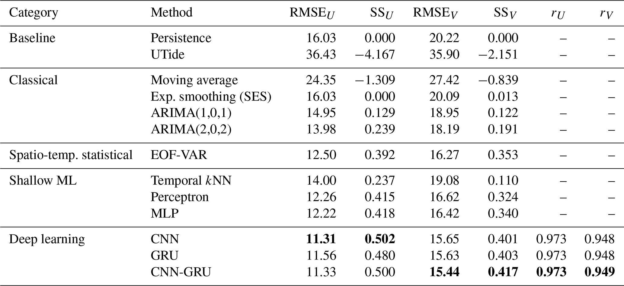
A clear, monotone performance hierarchy emerges (Fig. 9): deep learning (SS ≈ 0.40–0.50) > the reduced-rank spatio-temporal statistical model and shallow machine learning (EOF-VAR, perceptron, MLP; SS ≈ 0.32–0.42) > pointwise classical time series (ARIMA and kNN, SS ≈ 0.11–0.24) > persistence and exponential smoothing (SS ≈ 0) > the UTide and moving-average baselines (SS < 0), and this ordering holds for both velocity components. The contrast between EOF-VAR (SS_U = 0.39, SS_V = 0.35) and the pointwise ARIMA (SS_U = 0.13, SS_V = 0.12) is informative: introducing spatial correlation through a reduced-rank spatio-temporal statistical model recovers most of the gap to the neural networks, confirming that the dominant deficiency of the classical baselines is their neglect of spatial structure rather than of nonlinearity. The neural networks nonetheless retain a consistent edge over EOF-VAR (CNN-GRU SS_V = 0.42 vs. 0.35), attributable to their nonlinear spatio-temporal representation. All three deep learning models achieve overall correlation coefficients r>0.97 for U and r>0.94 for V (Table 2).

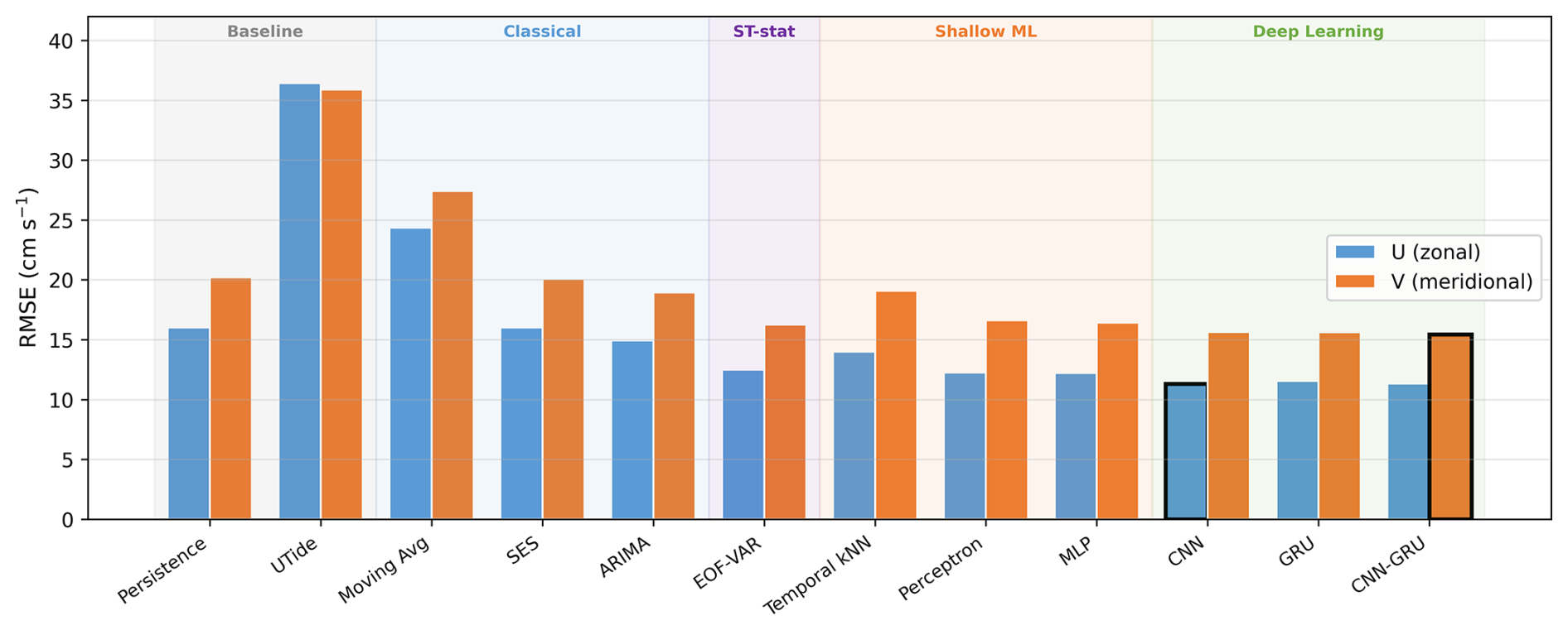
Figure 9 Phase 1 RMSE for all twelve methods, grouped by category. Bold outlines highlight the best model for each component.

The classical autoregressive models are competitive with persistence but do not approach the deep learning tier. The ARIMA and temporal kNN figures in Table 2 are evaluated on the full 291-cell domain over the entire test period: ARIMA(1,0,1) reaches 14.95 and 18.95 cm s⁻¹ (SS 0.13 and 0.12), worse for the meridional component than every deep learning model (CNN-GRU: 15.44 cm s⁻¹) and below the MLP. The order favoured by AIC within the low-order search is in fact (2,0,2) rather than (1,0,1) (54 of 60 cell-series; Sect. 3); even the AIC-optimal ARIMA(2,0,2) reaches only 13.98 and 18.19 cm s⁻¹ over the full domain, still well short of deep learning. Extending the order search to $p,q\le \mathrm{4}$ or adding a 12 h seasonal component does not materially improve out-of-sample accuracy (median RMSE changes of ≈2 % and ≈4 % on the diagnostics sample, respectively, with the mean change for the higher-order specifications being a slight degradation; Sect. 3), so this conclusion is not an artifact of the low-order specification. ARIMA's residuals retain significant autocorrelation at both orders (Ljung–Box p≈0 in essentially all cells), confirming that a per-cell low-order ARMA cannot capture the full tidal harmonic structure. The strong one-step autocorrelation of the tidal signal nonetheless allows ARIMA to exceed persistence, but temporal modelling alone does not match the spatio-temporal networks for either component.

The UTide baseline produces strongly negative skill scores (SS${}_U=-\mathrm{4.17}$). This is expected: for one-step prediction, persistence already contains the current tidal phase plus all non-tidal variability, while UTide relies on long-term harmonic fits that cannot capture the residual variability. We note that UTide predictions are also used for gap-filling (Sect. 2), so the UTide baseline is partially evaluated on data it helped generate; however, this would bias its RMSE downward, making the strongly negative skill scores a conservative estimate of its true limitation. The moving average fails (SS${}_U=-\mathrm{1.31}$) because averaging over the lookback window smooths the tidal oscillations.

Notably, the perceptron has the most parameters (1.81 M) of any Phase 1 model due to the large flattened input dimensionality ($T\times \mathrm{2}\times \mathrm{21}\times \mathrm{21}=\mathrm{2646}$ features × 512 units), yet performs worse than the CNN (1.34 M) and CNN-GRU (1.72 M). This indicates that, where it matters, architectural inductive bias rather than raw parameter count drives performance: the convolutional structure provides a spatial prior that fully connected layers cannot match. We caution, however, against over-generalising from the deep learning comparison: for one-step zonal prediction the CNN, GRU, and CNN-GRU are nearly indistinguishable (Table 2; five-seed $U=\mathrm{11.32}\pm \mathrm{0.05}$, 11.45±0.05, 11.32±0.04 cm s⁻¹), even though the GRU treats the grid as unstructured while the CNN is explicitly spatial. In this tidally dominated regime the repeating semidiurnal signal is strong enough that the choice of spatial architecture matters little for one-step U; spatial structure yields a measurable benefit chiefly for V, where along-strait gradients are steeper, and – as Phase 2 shows – when a longer lookback lets the hybrid exploit tidal-cycle phase.

The skill score comparison (Fig. 10) shows all deep learning models consistently achieving SS > 0.40.

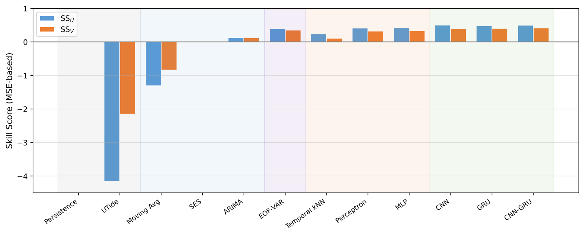
Figure 10 MSE-based skill scores relative to persistence for all methods. Positive values indicate improvement.

4.2 Phase 2: lookback sensitivity

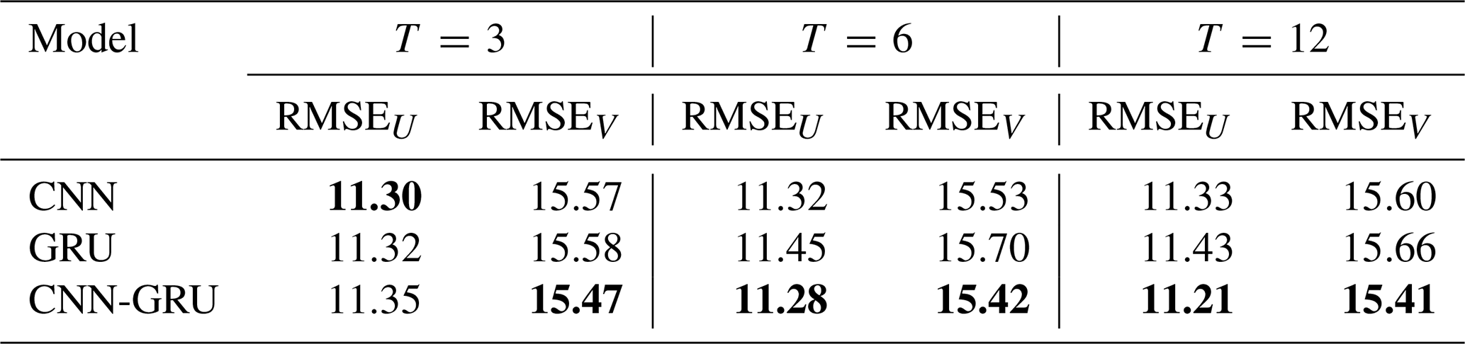
Figure 11 and Table 3 show the effect of lookback window length on the three deep learning architectures. Note that the CNN-GRU T = 3 values differ slightly between Phase 1 (Table 2: 11.33 cm s⁻¹) and Phase 2 (Table 3: 11.35 cm s⁻¹) due to independent training runs with different random seeds. The results reveal a clear architectural difference:

• CNN-GRU shows a monotonic trend: RMSE_U decreases from 11.35 (T = 3) to 11.28 (T = 6) to 11.21 cm s⁻¹ (T = 12), a 1.2 % improvement. RMSE_V shows a similar, though smaller, trend (15.47 → 15.42 → 15.41 cm s⁻¹). These differences are modest and comparable to the variation expected from stochastic training; however, the consistent direction across both components and all three lookback values suggests a real, if small, effect.

• The standalone CNN and GRU show no consistent benefit from longer lookbacks: CNN RMSE_U is essentially flat (11.30, 11.32, 11.33 cm s⁻¹). GRU performs slightly worse at longer lookbacks, possibly because additional input length introduces noise without commensurate spatial context.

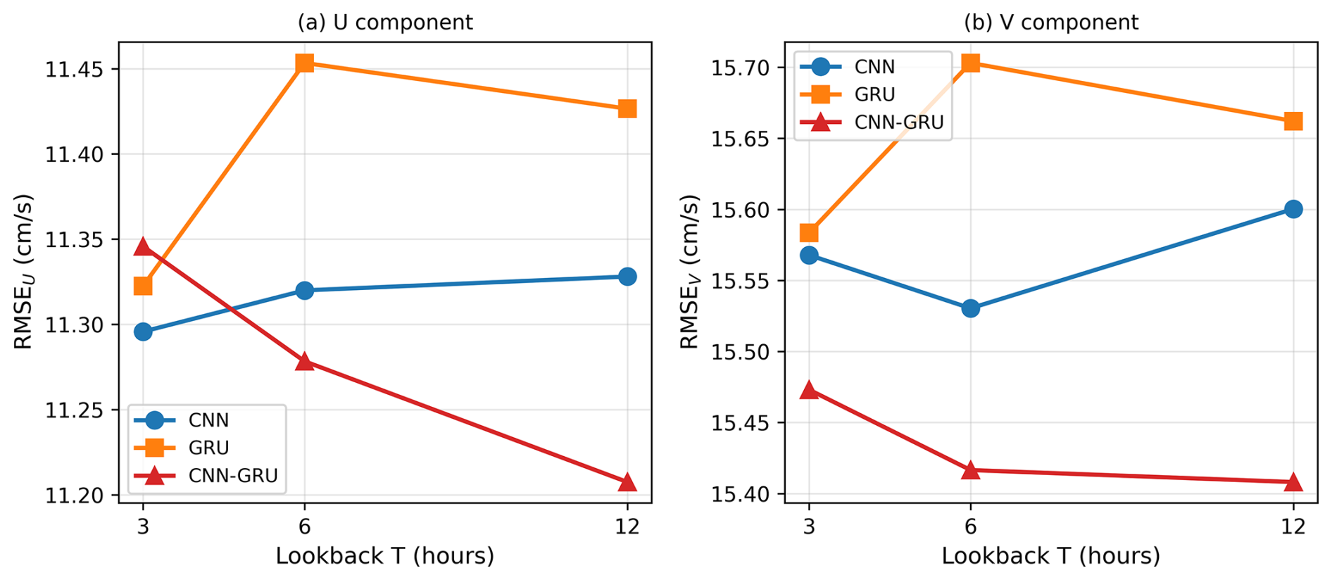
Figure 11 Phase 2: RMSE as a function of lookback window length for the three deep learning architectures. (a) U component. (b) V component.

Table 3 Phase 2: RMSE (cm s⁻¹) for deep learning models across lookback windows. Bold indicates the best result per column.

The CNN-GRU's monotonic improvement with lookback length indicates that the GRU component effectively integrates tidal phase information from longer sequences, while the CNN provides spatial context at each timestep. In contrast, the standalone GRU receives flattened frames without spatial structure, and the CNN stacks all frames along the channel dimension, which does not naturally model temporal ordering.

4.3 Phase 3: six-hour nowcasting

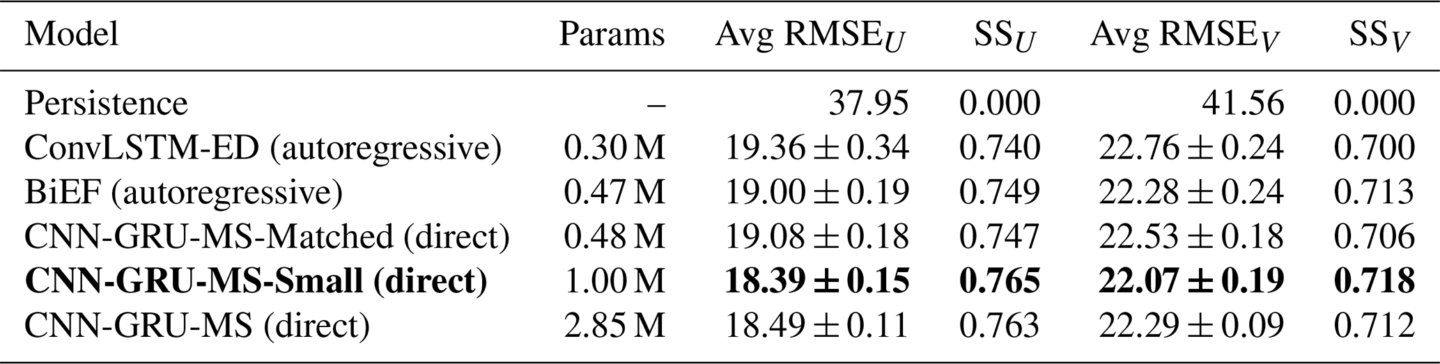
Table 4 reports the average RMSE across the six lead times for every multi-step model. To make the comparison free of platform, batch-size, and single-seed confounds, all five trainable models were retrained under an identical protocol – five random seeds, batch size 32, the same data, chronological splits, optimiser, and early-stopping criterion – on a single GPU (Sect. 3). Accuracy is governed primarily by model capacity: the 1.00 M-parameter CNN-GRU-MS-Small attains the lowest error (18.39±0.15 and 22.07±0.19 cm s⁻¹) and the 2.85 M full model is statistically identical (18.49±0.11 and 22.29±0.09 cm s⁻¹), so capacity beyond ∼ 1 M yields no further gain; error rises only at the smallest sizes. Critically, at matched capacity (∼ 0.48 M) the direct CNN-GRU-MS-Matched (19.08±0.18 and 22.53±0.18 cm s⁻¹) and the autoregressive BiEF (19.00±0.19 and 22.28±0.24 cm s⁻¹) are statistically indistinguishable: once capacity and training budget are equalised, direct multi-step prediction confers no accuracy advantage over autoregressive decoding. All models reduce the persistence mean square error by 70 %–77 % (skill scores 0.70–0.77).

Table 4 Phase 3: average RMSE (cm s⁻¹) over six lead times and MSE skill scores for multi-step nowcasting (T = 12), with model size. All five trainable models were retrained under an identical protocol (five seeds, batch 32, same splits, optimiser, and early stopping) on one GPU; values are five-seed means ± standard deviation. Bold indicates the lowest RMSE. The 0.48 M CNN-GRU-MS-Matched is capacity-matched to BiEF (0.47 M).

Although the architectures achieve comparable accuracy at matched capacity, they differ sharply in computational cost (Table 5), which is the decisive factor for operational deployment. The direct multi-step models train about 2.5 times faster – they emit all six steps in a single pass and converge in fewer epochs – and, more importantly for an operational nowcast, run roughly 4.5 times faster at inference, because the autoregressive models must decode the horizon step by step. A single direct model also covers all 291 cells, whereas the strongest classical baseline (per-cell ARIMA) requires fitting and maintaining 291 separate models.

Table 5 Phase 3 computational cost: per-seed training time (single NVIDIA RTX 5090 GPU) and CPU inference latency for one six-hour forecast (batch 1, single AMD Ryzen 7 7800X3D thread group). Absolute values are hardware-dependent and given for reference; the relative differences – the direct multi-step models are markedly cheaper on both axes – are hardware-independent.

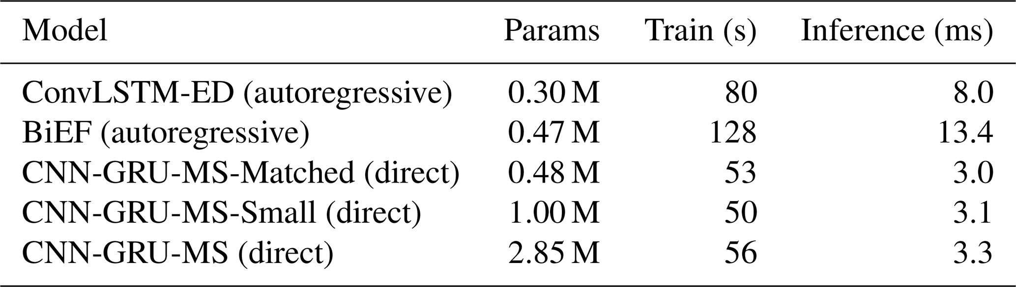
Figure 12 shows the RMSE degradation with lead time (a representative single-run profile; the controlled multi-seed averages are those in Table 4). Persistence RMSE grows from 16.0 cm s⁻¹ (t+1) to 56.4 cm s⁻¹ (t+6) for U – a factor of 3.5. The full CNN-GRU-MS degrades from 12.4 to 24.4 cm s⁻¹, a factor of only 2.0.

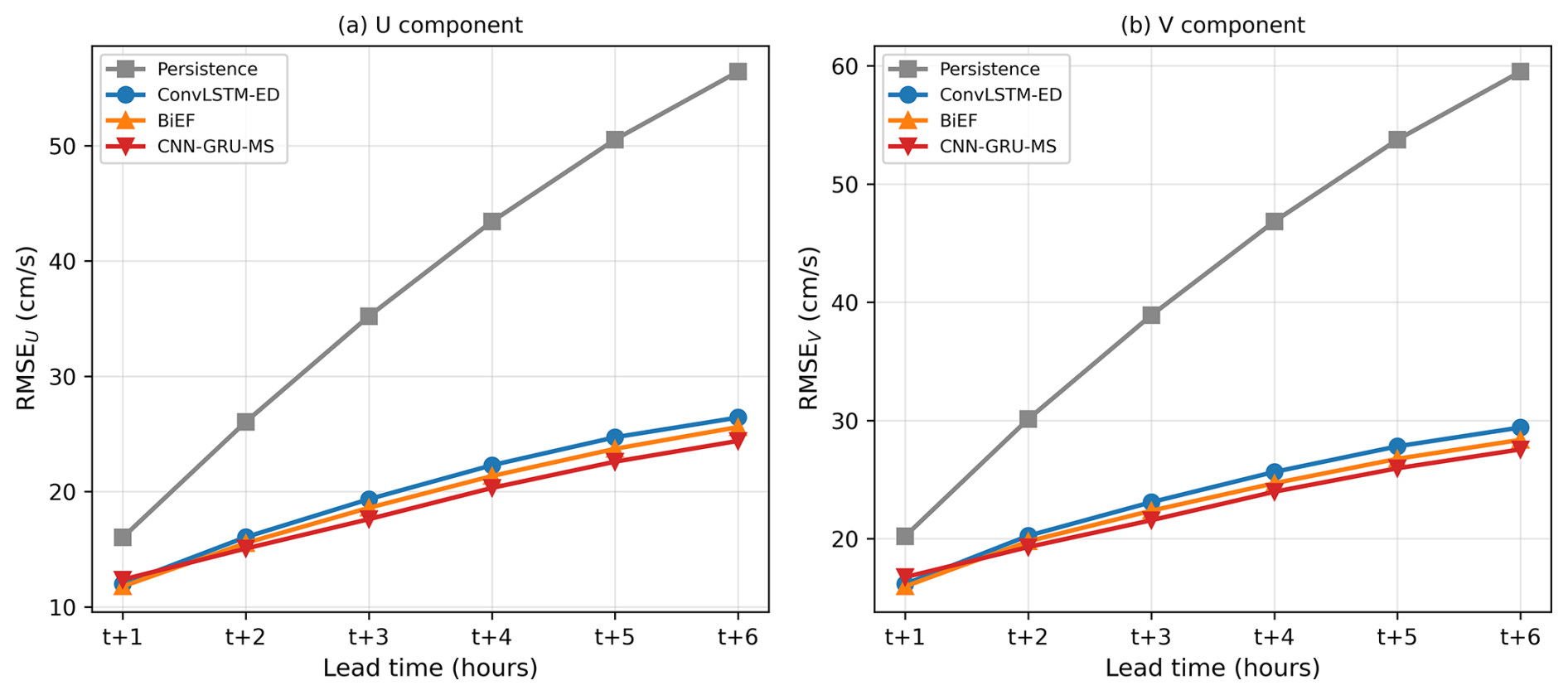
Figure 12 Phase 3: RMSE as a function of lead time for all nowcasting models. (a) U component. (b) V component.

A crossover occurs at t+1, where the autoregressive models (ConvLSTM-ED: 12.0 cm s⁻¹; BiEF: 11.8 cm s⁻¹) slightly outperform the full CNN-GRU-MS (12.4 cm s⁻¹) for U before the latter pulls ahead at longer leads. This reflects a genuine trade-off: autoregressive decoding can focus each step on one-step-ahead prediction (advantageous at short leads) but accumulates error over the horizon, whereas direct prediction distributes capacity across all six steps. We caution, however, that the full model's longer-lead advantage over BiEF in Fig. 12 partly reflects its six-fold larger capacity: at matched capacity the two strategies are statistically comparable (Table 4), so the operational case for the direct model rests on its much lower computational cost (Table 5) rather than on a lead-time accuracy advantage.

The per-lead-time skill scores (Fig. 13) show that all models maintain SS_U>0.4 at every lead time and SS_V>0.3. CNN-GRU-MS reaches SS_U = 0.81 at t+6, reducing 81 % of the persistence mean square error even at the longest forecast horizon.

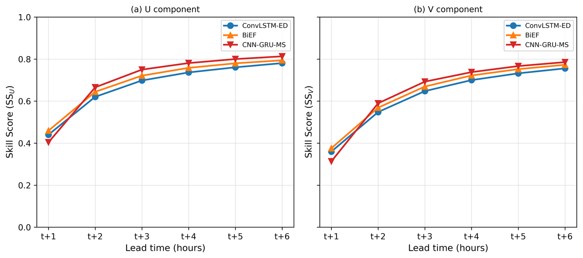
Figure 13 Phase 3: per-lead-time skill score relative to step-k persistence. (a) U component. (b) V component.

BiEF outperforms ConvLSTM-ED at all lead times, with the advantage increasing from 0.2 cm s⁻¹ at t+1 to 0.8 cm s⁻¹ at t+6 for U, indicating that bidirectional encoding provides a richer initial state for the decoder.

4.4 Diurnal error analysis

Figure 14 shows the one-step RMSE (Phase 1) stratified by hour of day. The Sunda Strait is at approximately 105° E (UTC+7). The elevated-error period (06:00–18:00 UTC) corresponds to 13:00 to 01:00 LT (following day). The difference between high-error and low-error periods is visually evident across all models.

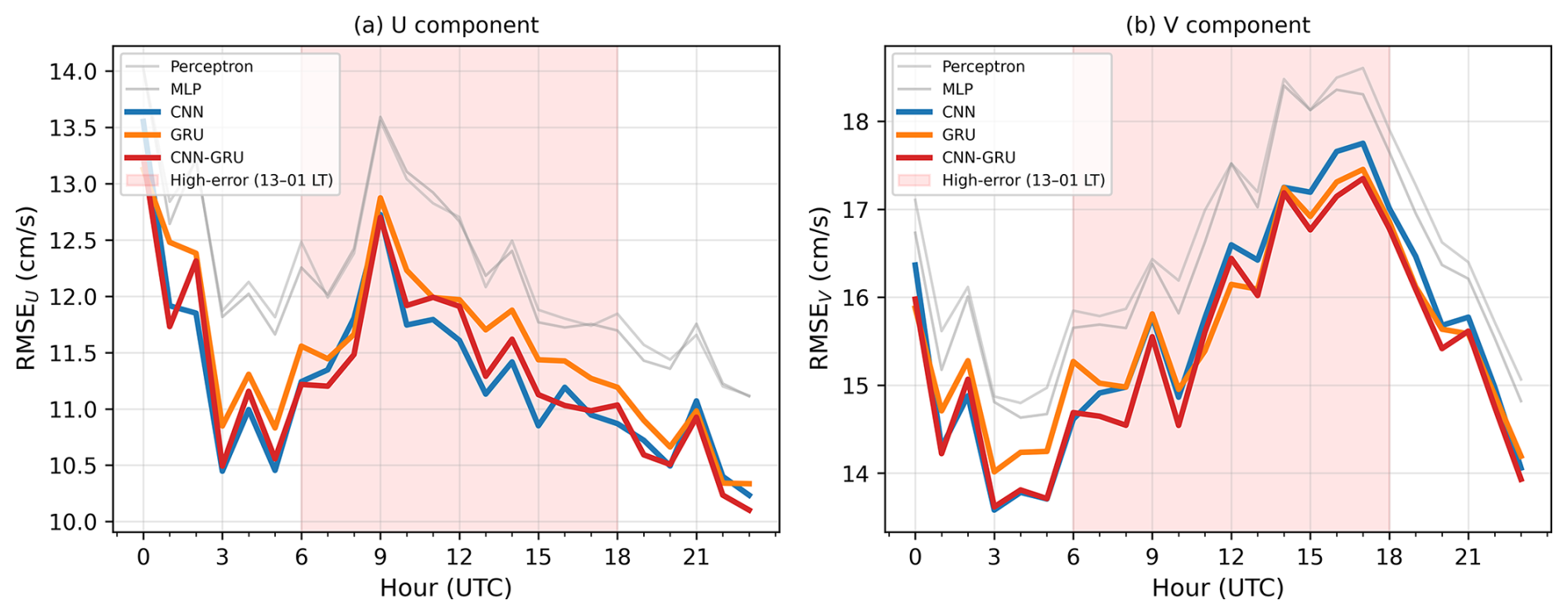
Figure 14 Diurnal RMSE pattern for the five neural network models (Phase 1). Red shading indicates the high-error period (06:00–18:00 UTC, corresponding to 13:00–01:00 LT). (a) U component. (b) V component.

To investigate the physical driver, we compare the diurnal RMSE pattern with concurrent wind observations from the three AWS stations at Merak, Ciwandan, and Bakauheni (Fig. 15). The three-station average wind speed shows a clear sea-breeze signal, peaking at ∼4.8 m s⁻¹ near 15:00 LT (08:00 UTC) and dropping to ∼3.0 m s⁻¹ at night. However, the relationship between the diurnal cycles of wind speed and model RMSE – measured as a Spearman rank correlation across the 24 hourly bins, so the associated p-values are indicative rather than strict given the smooth, autocorrelated diurnal shape and small effective sample – differs by component: for U, the correlation is positive (r_s = 0.48, nominal p = 0.018), consistent with sea-breeze-driven zonal surface currents degrading prediction skill. For V, it is negative ($r_{\mathrm{s}}=-\mathrm{0.41}$), so the elevated meridional errors are not explained by wind speed and instead follow a separate diurnal cycle.

We examine this component split directly by projecting the three-station AWS wind onto the strait axis – oriented NE–SW, the principal axis of the observed current variability (Sect. 4.7) – and regressing the diurnal component errors on the along- and cross-strait wind. The zonal (U) error scales with total wind speed (r_s = 0.48) more strongly than with either signed projection (r_s = 0.04 cross-strait, 0.36 along-strait), consistent with the afternoon sea breeze injecting unmodelled, current-only-unpredictable momentum that raises U error when the wind is strongest. The meridional (V) error, in contrast, is negatively correlated with wind speed ($r_{\mathrm{s}}=-\mathrm{0.41}$) yet positively correlated with both the along- and cross-strait wind projections (r_s = 0.64 and 0.76). The decisive feature is the sign with respect to speed: wind drag should grow as the wind strengthens, yet the V error falls when the wind is strongest, its diurnal minimum coinciding with the afternoon sea-breeze maximum. The positive correlation with both orthogonal projections is consistent with – though it does not by itself prove – a shared diurnal cycle rather than direct forcing, since both projections also peak with the afternoon sea breeze; the speed-negative relationship and the tidal-phase timing are the cleaner diagnostics. Taken together, and bearing in mind that these are descriptive correlations over 24 diurnal bins, the evidence is most consistent with the apparent negative V-wind correlation being a tidal-phase coincidence: the meridional error – systematically the harder component across all methods and phases – appears dominated by tidal dynamics rather than by wind forcing.

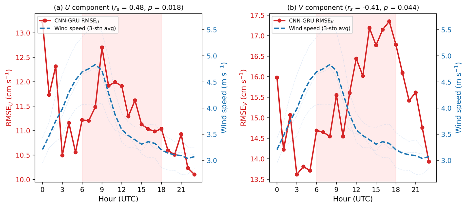
Figure 15 Diurnal RMSE (red, left axis) overlaid with three-station average wind speed (blue dashed, right axis). Red shading marks the high-error period (06:00–18:00 UTC, corresponding to 13:00–01:00 LT). (a) U component. (b) V component.

All five neural network models exhibit the same diurnal modulation, indicating a physical limitation rather than a model-specific artefact.

4.5 Seasonal error stratification

To assess the influence of monsoon regime on prediction skill, Phase 1 test-set errors for persistence, ARIMA(1,0,1), and the three deep learning models are stratified into three seasons: the southeast (SE) monsoon (July–August), the transition period (September–November), and the northwest (NW) monsoon (December–February). Table 6 summarises the results; ARIMA is stratified over the full domain and period, consistently with the other methods.

Table 6 Seasonal RMSE (cm s⁻¹) for persistence, ARIMA(1,0,1), and the three deep learning models (Phase 1, T = 3). Bold indicates the lowest RMSE per season. ARIMA's lowest-error season is the SE monsoon.

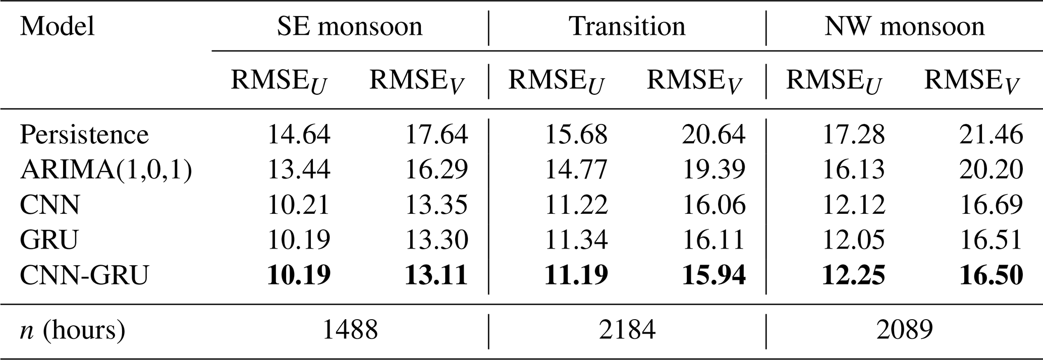
All models show a consistent seasonal dependence: RMSE is lowest during the SE monsoon (U: 10.19 cm s⁻¹, V: 13.11 cm s⁻¹ for CNN-GRU) and highest during the NW monsoon (U: 12.25 cm s⁻¹, V: 16.50 cm s⁻¹), representing a 20 % (U) and 26 % (V) seasonal increase in error. The NW monsoon brings stronger and more variable winds from the Java Sea (Wyrtki, 1961), introducing non-tidal surface current variability that is not captured by models trained predominantly on tidal dynamics. Persistence and ARIMA errors follow the same seasonal pattern, confirming that the increased NW monsoon error reflects genuinely harder-to-predict dynamics rather than model degradation. ARIMA's lowest-error season is the SE monsoon (V=16.29 vs. 18.95 cm s⁻¹ over the full period), consistent with the stronger non-tidal forcing of the NW monsoon being the principal source of seasonal error growth.

4.6 Tidal–residual error decomposition

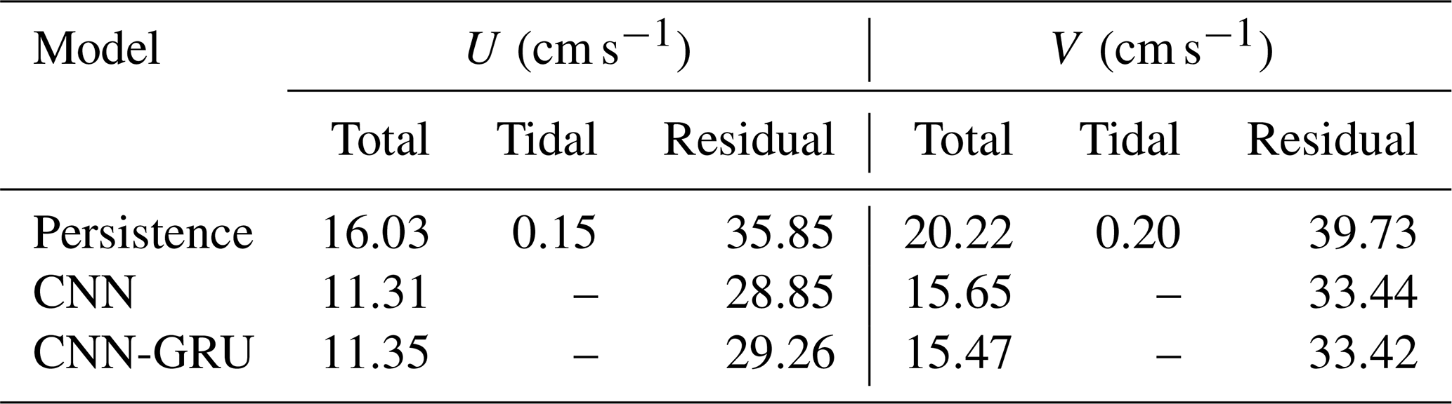
To quantify the contribution of tidal versus non-tidal variability to prediction errors, we decompose the observed current at each grid point into a tidal component (predicted by UTide fitted to the training period) and a residual. Table 7 presents the results. For persistence, the tidal RMSE is negligible (<0.2 cm s⁻¹) because the tidal signal changes minimally over a one-hour lag. Nearly all persistence error arises from the residual component (35.8 and 39.7 cm s⁻¹). CNN and CNN-GRU reduce residual-component errors by 19 %–20 % (U) and 16 % (V) relative to persistence (GRU is omitted because it lacks the CNN encoder needed to isolate spatial contributions), indicating that they capture some non-tidal variability – likely wind-driven and sub-tidal fluctuations – beyond the deterministic tidal signal. However, the residual RMSE remains substantially larger than the total RMSE (28.9 vs. 11.3 cm s⁻¹ for CNN), reflecting the well-known challenge of predicting mesoscale and sub-mesoscale ocean variability.

Table 7 Tidal–residual error decomposition for one-step prediction (T = 3). Tidal RMSE measures the error in the tidal component of each prediction; residual RMSE measures the error in the non-tidal component. CNN and CNN-GRU total RMSE values differ slightly from Table 2 (by ≤0.03 cm s⁻¹) because the tidal decomposition uses an independent training run.

This decomposition also lets us test, rather than assert, the nature of ARIMA's skill. We split each cell's series into the UTide tidal component and a non-tidal residual and re-fit the ARIMA(1,0,1) directly to each band. The deterministic tide changes by only ∼0.07 cm s⁻¹ over a one-hour lag in this decomposition (consistent with the under-0.2 cm s⁻¹ persistence tidal RMSE in Table 7), so it is trivially predictable at one step; consequently persistence's one-step error on the raw series (16.0 and 20.2 cm s⁻¹ for U and V) is essentially identical to its error on the residual alone (16.0 and 20.2 cm s⁻¹) – the one-step error is almost entirely sub-tidal. An ARIMA fitted directly to that residual achieves zero skill over persistence (skill score 0.00 for U and −0.02 for V; RMSE 16.0 and 20.4 versus persistence's 16.0 and 20.2 cm s⁻¹). ARIMA's modest edge over persistence on the raw series (full-domain SS ≈ 0.13 and 0.12) therefore derives entirely from the smooth, strongly autocorrelated tidal oscillation that its AR and MA terms track slightly better than naive persistence, and not from any ability to predict the sub-tidal residual that dominates the total error. This is corroborated by the Ljung–Box tests (Sect. 3), which show ARIMA residuals retain significant autocorrelation at the tidal periods, and by the strongly negative skill of the pure-harmonic UTide baseline (Table 2): the deterministic tide alone, without the autoregressive persistence term, is insufficient. These results directly confirm and qualify the tidal-autocorrelation interpretation – temporal autocorrelation explains ARIMA's skill, but that skill is small once the comparison is made over the full domain and period. (ARIMA is not listed as a row in Table 7 because that table scores total-field predictions against the deterministic tidal field, whereas the per-cell autoregressive forecast is decomposed by re-fitting to each band as described here.)

4.7 Spatial error distribution

Figure 16 shows the per-cell RMSE for the three Phase 1 deep learning models. All three models exhibit a consistent spatial pattern: errors are lowest in the central domain (RMSE_U≈6–8 cm s⁻¹, RMSE_V≈10–12 cm s⁻¹) and increase toward the strait boundaries, particularly in the northwest and southeast corners where current speeds and spatial gradients are highest. The V component shows elevated errors along the northeast–southwest axis (the along-strait direction), consistent with the stronger tidal amplification of meridional currents.

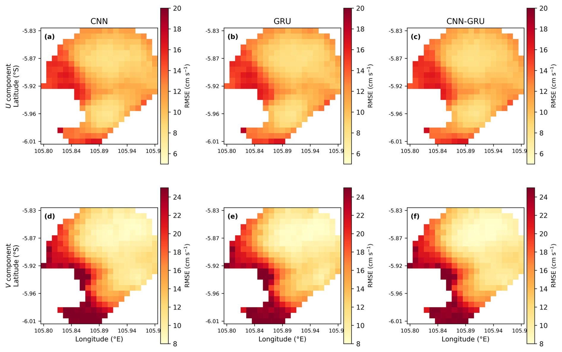
Figure 16 Spatial distribution of per-cell RMSE for the three Phase 1 deep learning models. Top row: U component. Bottom row: V component. Higher errors occur near the strait boundaries where current gradients are steepest.

The spatial error pattern is remarkably similar across all three architectures, suggesting that the error distribution is governed by the underlying physical dynamics (tidal amplification near boundaries, coastal interactions) rather than by model-specific limitations. Mean per-cell correlation coefficients are high across all models (0.97 for U, 0.93 for V), with slightly lower values near the domain edges where the signal-to-noise ratio of the HF radar measurements is also lower.

To test whether this spatial structure is intrinsic to the physics or specific to the deep learning models, we computed the per-cell RMSE map of the pointwise ARIMA model and correlated it with the deep learning maps (Fig. 17). The spatial patterns are nearly identical: the ARIMA error map correlates with the CNN, GRU, and CNN-GRU maps at r = 0.96–0.98 for U and 0.98 for V. A purely temporal, per-cell statistical model and the spatio-temporal networks therefore share the same error geography – low in the interior, high in the NW and SE corners – confirming that the spatial distribution of error is set by the tidal dynamics (amplification and steep gradients near the boundaries) rather than by model class. This is consistent with the expectation (Sect. 5) that a dedicated spatio-temporal statistical model would inherit the same error geography while improving the overall level of skill toward the neural networks.

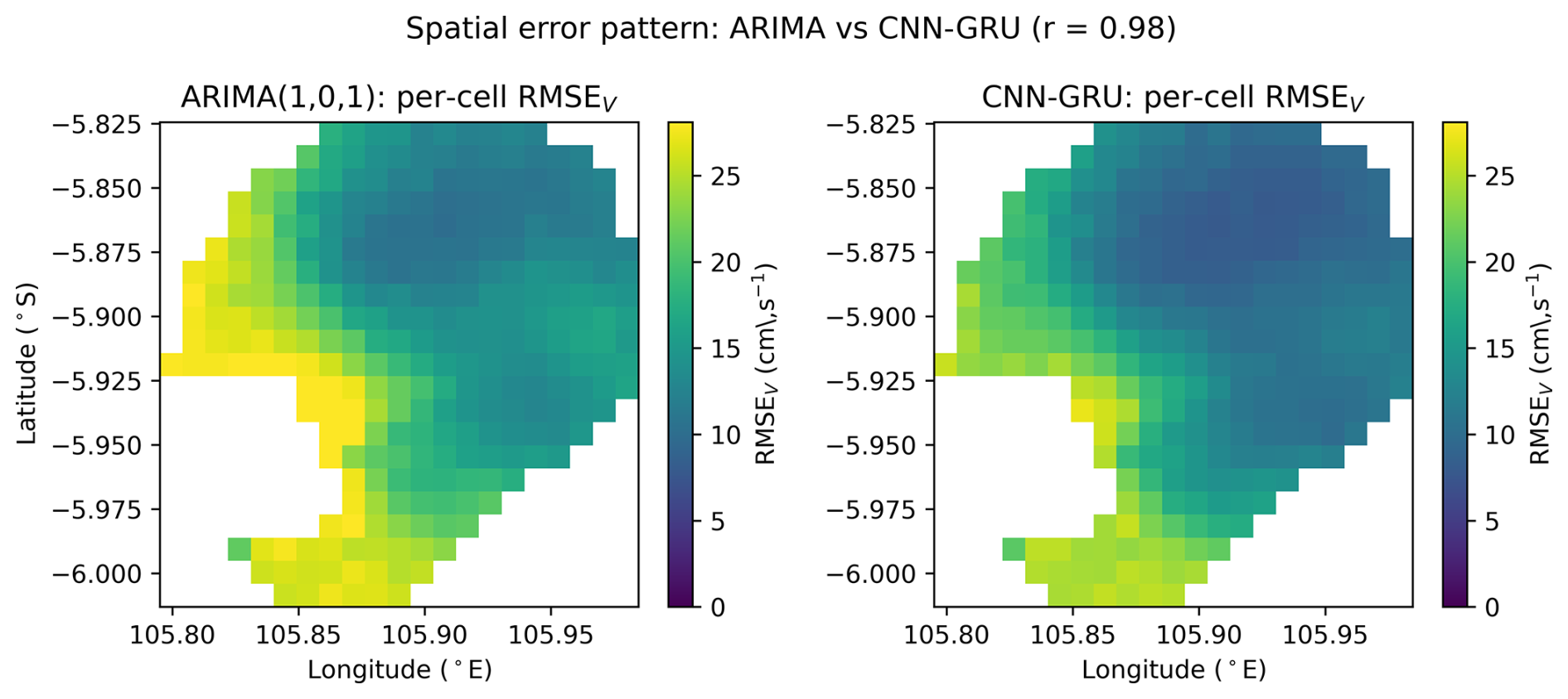
Figure 17 Per-cell meridional RMSE for the pointwise ARIMA(1,0,1) model (left) and the spatio-temporal CNN-GRU (right). Despite ARIMA's higher overall error, the two maps share the same spatial structure (r = 0.98), indicating that the error geography is governed by the tidal dynamics rather than by model class.

4.8 Gap-filled versus observed performance

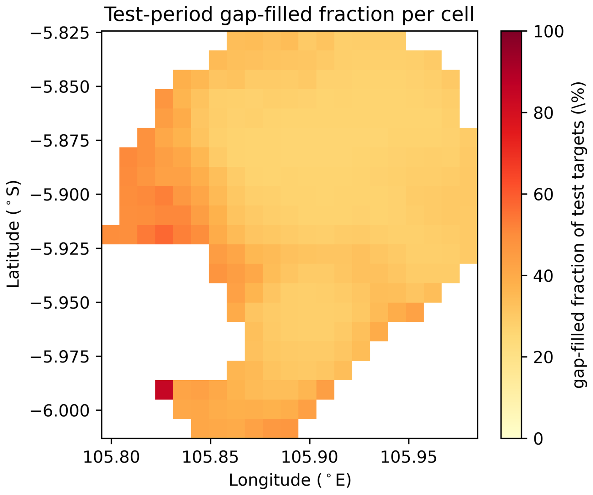
Because ∼15 % of the full record is gap-filled with UTide tidal predictions (Sect. 2), and HF-radar gaps cluster in the low-quality boundary regions where errors are also highest, we examined whether the reported skill is contaminated by models reproducing the deterministic gap-fill. Over the test period the sea-cell gap fraction is 32.9 % (higher than the whole-record average because coverage is lower in this window), and it is higher at the 88 boundary cells (38.0 %) than in the interior (30.6 %). Splitting the test targets into genuinely-observed and gap-filled, every method has lower error on the gap-filled targets (e.g. CNN V: 12.5 cm s⁻¹ gap-filled vs. 16.8 observed; persistence V: 17.8 vs. 21.3; ARIMA V: 15.9 vs. 20.3 cm s⁻¹), because the UTide gap-fill is smooth and tidally deterministic and therefore easier to predict. Including gap-filled targets thus slightly deflates the reported RMSE; the observation-only values – the honest measure of skill against real data – are modestly higher (e.g. CNN V: 16.8 vs. the 15.65 cm s⁻¹ all-target value). The ranking of methods is unchanged under either split. The per-cell gap fraction is mapped in Fig. 18; comparison with the error map (Fig. 16) confirms that the gap-rich boundary cells are also the high-error cells. We recommend the observation-only metric for operational assessment.

Figure 18 Fraction of test-period targets that are gap-filled (UTide), per sea cell. The gap fraction is higher near the strait boundaries (38.0 % at edge cells) than in the interior (30.6 %), coinciding with the high-error regions in Fig. 16.

4.9 Vector-valued error metrics

Because tidal currents rotate, evaluating U and V separately does not reveal whether a model reproduces the direction of the flow – the quantity most relevant to trajectory forecasting and search-and-rescue. The Sunda Strait tidal current is strongly rectilinear along the NE–SW strait axis (Sect. 4.7), so the dominant rotary structure is a semidiurnal reversal along that axis rather than a smoothly rotating ellipse. We therefore complement the component RMSE with three vector-aware metrics over the test set (Table 8): the speed RMSE $\sqrt{\langle \left(\right|\widehat{\mathit{u}}|-|\mathit{u}|{)}^{\mathrm{2}}\rangle }$, the vector (complex) RMSE $\sqrt{\langle |\widehat{\mathit{u}}-\mathit{u}{|}^{\mathrm{2}}\rangle }$, and the direction mean absolute error (evaluated where the observed speed exceeds 10 cm s⁻¹).

Table 8 Vector-valued error metrics over the test set (all sea cells): speed RMSE, vector (complex) RMSE, and direction mean absolute error (computed where observed speed >10 cm s⁻¹). The deep learning models reproduce the flow direction substantially better than persistence or ARIMA. Bold indicates the best value.

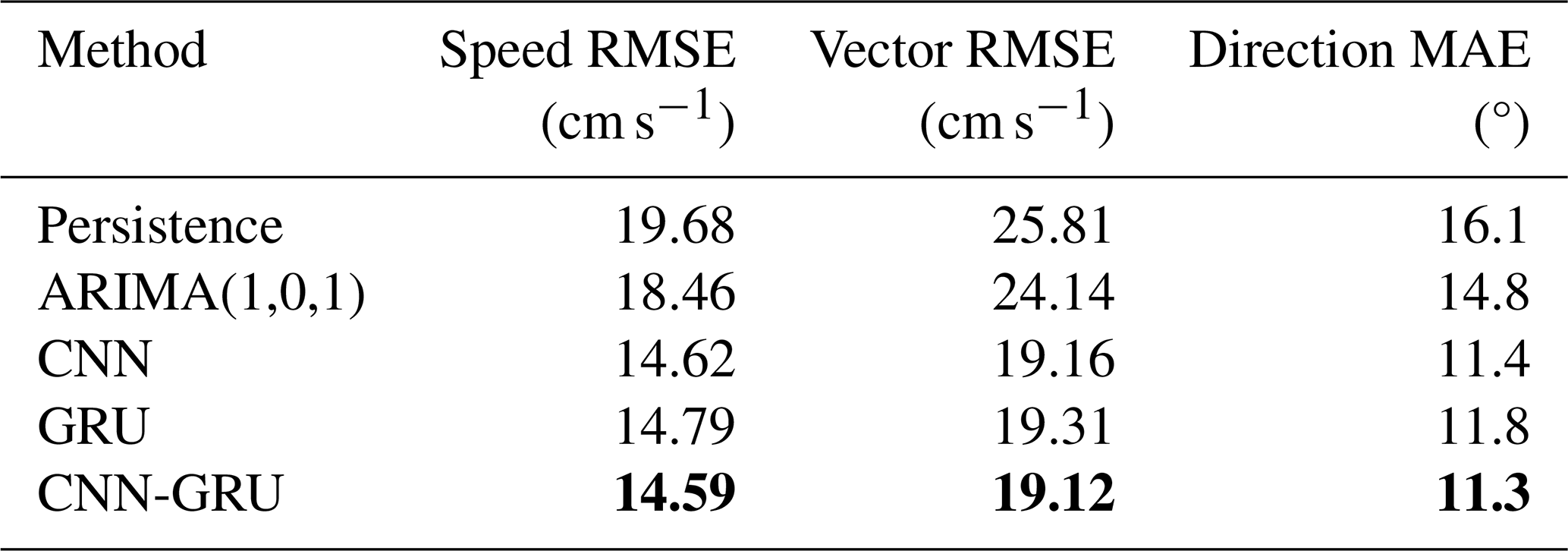
The deep learning models cut the direction error to ∼11–12°, against 16.1° for persistence and 14.8° for ARIMA, and similarly reduce the speed and vector RMSE by ∼25 %. ARIMA exhibits a negative speed bias (−3.5 cm s⁻¹), under-predicting current magnitude as expected for a mean-reverting model, whereas persistence is approximately unbiased in speed. Thus the deep learning advantage seen in the component RMSE carries over to the operationally relevant full-vector error: the networks reproduce both the magnitude and the direction of the surface current more faithfully than the statistical baselines.

5 Discussion

5.1 Performance in energetic strait environments

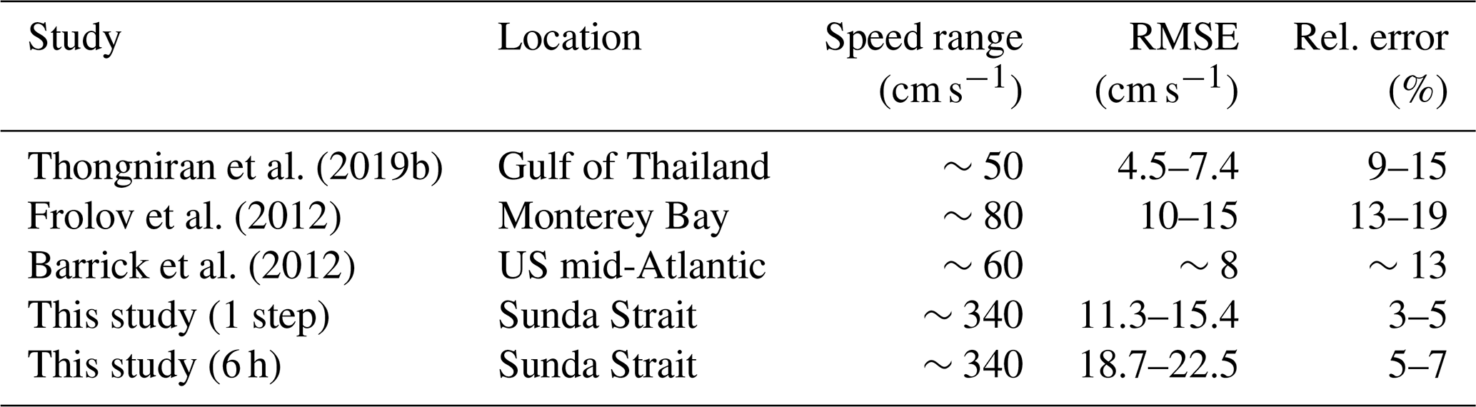
The absolute RMSE values in this study are higher than those reported in open-sea environments: 4.5–7.4 cm s⁻¹ in the Gulf of Thailand (Thongniran et al., 2019b), 10–15 cm s⁻¹ in Monterey Bay (Frolov et al., 2012), and ∼8 cm s⁻¹ along the US mid-Atlantic coast (Barrick et al., 2012). This reflects the much stronger tidal dynamics in the Sunda Strait (Table 9). When normalised by the observed speed range (defined here as the maximum minus minimum of the respective velocity component at each site), relative errors of 3 %–7 % are of the same order as those in other environments (Table 9). We stress that this normalisation is a first-order framing device, not evidence of superior performance: the low percentage is in large part a mathematical consequence of dividing by the Sunda Strait's very large speed range (nearly seven times that of the smallest comparison site), and the metric does not account for differences in spatial resolution, temporal resolution, prediction horizon, or the (study-dependent) definition of “speed range”. Given these methodological differences, the comparison should be read only as indicating that deep learning does not break down in an energetic strait, not as a quantitative ranking against the cited studies.

Thongniran et al. (2019b)Frolov et al. (2012)Barrick et al. (2012)

Table 9 Comparison with previous HF radar current prediction studies.

5.2 Tidal cycle coverage in the lookback window

Phase 2 reveals that only the CNN-GRU benefits from longer lookbacks. This has a clear physical interpretation: the M2 tidal period is ∼12.42 h, so T=12 provides the GRU with approximately one full tidal cycle. The CNN-GRU exploits this because the GRU naturally processes ordered sequences and can learn the tidal phase–amplitude relationship, while the CNN provides spatial context at each step. In contrast, the standalone CNN stacks all frames along the channel axis, destroying temporal ordering, and the standalone GRU receives flattened spatial fields, losing the spatial structure needed to benefit from longer sequences.

The modest improvement from T=3 to T=12 for one-step prediction (1.2 % for U) is consistent with the high autocorrelation at one-hour lag. The effect is amplified for multi-step prediction, where knowledge of the full tidal cycle provides phase information essential for forecasts extending several hours ahead.

One caveat is that temporal gaps (∼15 % of hours) are filled using UTide tidal harmonic predictions prior to model training (Sect. 2). While this ensures gap-free lookback sequences for all models, it could artificially inflate the apparent benefit of longer lookbacks by providing smoother (tidal-only) inputs at gap-filled timesteps. The effect is mitigated by the fact that the same gap-filling is applied across all lookback lengths, so the relative comparison remains valid. Future work could evaluate models robust to missing inputs as an alternative to gap filling.

5.3 Autoregressive versus direct multi-step prediction

A controlled comparison – all five multi-step models retrained over five seeds with an identical batch size, optimiser, and early-stopping criterion on a single GPU (Table 4) – shows that model capacity, not the direct-versus-autoregressive distinction, governs accuracy. Error decreases with capacity up to ∼1 M parameters and then plateaus: CNN-GRU-MS-Small (1.00 M) is the most accurate (18.39 and 22.07 cm s⁻¹) and is statistically tied with the 2.85 M full model. At matched capacity (∼0.48 M) the direct CNN-GRU-MS-Matched (19.08 and 22.53 cm s⁻¹) and the autoregressive BiEF (19.00 and 22.28 cm s⁻¹) are statistically indistinguishable – all differences lie within the five-seed standard deviation (∼0.2 cm s⁻¹). Error accumulation in the autoregressive decoder is, at this six-hour horizon, offset by the autoregressive models' ability to focus each step on one-step-ahead prediction. The t+1 crossover – where autoregressive models slightly outperform CNN-GRU-MS – suggests that autoregressive decoding retains an advantage at the shortest lead. A hybrid strategy (autoregressive for t+1, direct for longer leads) could in principle exploit this, but the operational complexity is unlikely to justify the marginal improvement. BiEF consistently outperforms ConvLSTM-ED, confirming that bidirectional encoding provides a richer initial state for the decoder.

5.4 The V component is systematically harder to predict

Across all methods and phases, V RMSE exceeds U RMSE by 30 %–50 %. In the Sunda Strait (oriented NE–SW), the meridional component is approximately aligned with the along-strait direction where tidal amplification is strongest. The wider dynamic range (394 cm s⁻¹ for V versus 339 cm s⁻¹ for U) and steeper spatial gradients near coastal boundaries make V inherently more difficult to predict.

5.5 Computational efficiency

The multi-step architectures achieve comparable accuracy at matched capacity, but they differ markedly in computational cost (Table 5), which is the decisive factor for operational deployment. Producing the full six-hour horizon in a single forward pass, the direct CNN-GRU-MS trains about 2.5 times faster (it converges within the early-stopping budget, whereas BiEF did not early-stop within the 20-epoch cap) and runs about 4.5 times faster at inference – 3.0 vs. 13.4 ms per forecast on a single CPU (Table 5) – because the autoregressive models must decode the six steps sequentially. For an hourly operational nowcast all models are fast enough in absolute terms (≪1 s), so inference latency is not itself a binding constraint; the direct model's advantages are its lower training cost (relevant for periodic retraining), its lower inference cost (relevant for scaling to larger grids, higher update frequencies, or constrained CPU-only hardware), and the fact that a single model covers all 291 cells – whereas the per-cell classical baselines (e.g. ARIMA) require fitting and maintaining one model per grid point. On this basis we recommend the 1.00 M CNN-GRU-MS-Small, which attains the best accuracy at the smallest size, for operational deployment.

5.6 Classical baselines and spatio-temporal statistical models

The pointwise classical baselines in this study (moving average, exponential smoothing, ARIMA, temporal kNN) are deliberately univariate, per-cell models that ignore spatial correlation. To test directly whether their deficit relative to the neural networks is due to neglected spatial structure or to the absence of nonlinearity, we benchmarked them against an explicitly spatio-temporal statistical model: the EOF-VAR reduced-rank dynamic spatio-temporal model (Cressie and Wikle, 2011; Wikle et al., 2019) described in Sect. 3, which represents spatial covariance through empirical orthogonal functions and temporal dynamics through a vector autoregression on the leading principal components. EOF-VAR (SS_U = 0.39, SS_V = 0.35) substantially outperforms the pointwise ARIMA (SS_U = 0.13, SS_V = 0.12) and reaches the shallow-machine-learning tier, recovering most of the gap to the neural networks. This decisively attributes the classical methods' deficit to their neglect of spatial correlation: once a linear statistical model is allowed to share information across space, it becomes competitive. The neural networks nonetheless retain a consistent advantage (CNN-GRU 11.33/15.44 vs. EOF-VAR 12.50/16.27 cm s⁻¹), which we attribute to their nonlinear representation of the spatio-temporal field; and consistently with this, the per-cell error geography is shared across the pointwise ARIMA and the spatio-temporal networks (r = 0.96–0.98; Sect. 4.7). Extending EOF-VAR or a full integro-difference-equation model to the multi-step setting of Phase 3, and incorporating nonlinear basis functions, are natural directions for future work.

5.7 Limitations

Several limitations should be noted. First, although the Phase-1 deep learning models and all five Phase-3 multi-step models are evaluated over five seeds (standard deviations 0.03–0.34 cm s⁻¹), the Phase-2 lookback trends (0.06–0.14 cm s⁻¹) are comparable to this variability and should be interpreted with caution. Second, the lead-time breakdown (Fig. 12) is shown for a representative single run; the controlled multi-seed comparison is summarised by the lead-time-averaged values in Table 4, and the training-time and inference-latency figures (Table 5) are reported for the specific hardware listed and should be read as relative rather than absolute. Third, a substantial fraction of timesteps are gap-filled using UTide tidal predictions (∼15 % of the full record, but 32.9 % of sea-cell test targets; Sect. 4.8); models trained on these partially synthetic inputs may learn smoother-than-observed dynamics. As shown in Sect. 4.8, errors are lower on gap-filled targets for all methods, so all-target RMSE slightly understates the error against genuine observations; we therefore also report the observation-only RMSE and recommend it for operational assessment. Fourth, all models receive only the recent current history; incorporating external forcing (tidal predictions, wind, atmospheric pressure) could improve skill during sea-breeze-affected periods. Fifth, the study uses a single HF radar system covering a ∼900 km² area; generalisation to other settings requires validation. Sixth, models predict at the 291 observed grid points only; extending predictions to the 137 blind-zone cells or beyond the radar footprint requires additional spatial reconstruction methods.

6 Conclusions

This study presents a three-phase evaluation of forecasting methods for HF radar surface currents in the Sunda Strait, progressing from one-step prediction to six-hour nowcasting. The main findings are as follows.

1. Among twelve methods for one-step prediction, evaluated consistently over all 291 cells and the full test period, the deep learning models achieve the highest skill for both components (CNN, SS_U = 0.50, r>0.97; CNN-GRU, SS_V = 0.42). Five-seed experiments confirm that CNN and CNN-GRU are statistically indistinguishable for U (11.32±0.05 and 11.32±0.04 cm s⁻¹), reflecting that the dominant semidiurnal signal renders the spatial-architecture choice nearly immaterial for one-step zonal prediction. The pointwise classical models (ARIMA, exponential smoothing, kNN) exceed persistence but fall well below deep learning; a reduced-rank spatio-temporal statistical model (EOF-VAR) that accounts for spatial correlation recovers most of the gap (SS_U = 0.39, SS_V = 0.35), showing that the classical deficit is dominated by the neglect of spatial structure rather than of nonlinearity.

2. CNN-GRU is the only architecture that improves with longer lookback (T = 3 to 12 h), demonstrating unique exploitation of tidal cycle information. Standalone CNN and GRU show no benefit.

3. For six-hour nowcasting, multi-step accuracy is governed by model capacity, plateauing near 1 M parameters (CNN-GRU-MS-Small: 18.39±0.15 and 22.07±0.19 cm s⁻¹; SS 0.77 and 0.72). Under a controlled five-seed comparison the direct and autoregressive architectures are statistically indistinguishable at matched capacity (∼0.48 M: direct 19.08/22.53 versus BiEF 19.00/22.28 cm s⁻¹). The direct multi-step CNN-GRU-MS is nonetheless preferred for operational nowcasting because it trains ∼2.5 times faster and runs ∼4.5 times faster at inference (a single forward pass versus sequential decoding).

4. All models exhibit a diurnal error pattern. Concurrent AWS wind observations show that the zonal (U) error increase correlates with afternoon sea-breeze enhancement (r_s = 0.48 across the 24 diurnal-mean hours), while the meridional (V) diurnal pattern is not wind-driven and likely reflects tidal phase effects.

5. Relative errors of 3 %–7 % of the observed speed range are of the same order as those in calmer environments, suggesting that deep learning generalises to energetic strait settings, though this normalisation partly reflects the strait's very large speed range and cross-site comparisons are further limited by differences in resolution and prediction horizon.

Beyond the site-specific results, four methodological insights may generalise to other HF radar forecasting applications: (i) tidal harmonic models, despite their physical basis, do not outperform persistence at one-step-ahead horizons where autocorrelation dominates, cautioning against the assumption that physics-based baselines are always superior; (ii) the lookback window length matters only when the architecture can jointly exploit spatial and temporal structure; (iii) at matched capacity, direct and autoregressive multi-step architectures achieve comparable accuracy – so a controlled, capacity-matched comparison rather than a headline RMSE is needed to compare architectures, and the direct model's advantage is computational (faster training and single-pass inference) rather than one of accuracy; and (iv) baselines must be evaluated on the same spatial domain and time span as the models they are compared against, since a spatially or temporally restricted evaluation can flatter a per-cell baseline and invert the apparent ranking.

The direct multi-step CNN-GRU-MS combines the best forecast skill with the lowest computational cost, making it a promising candidate for operational nowcasting in tidally dominated strait environments.