Asymptotically-unbiased nonparametric estimation of the power spectral density from uniformly-spaced data with missing samples

The nonparametric estimation of the power spectral density of uniformly-spaced data with missing samples is revisited. Classical estimators, such as the standard periodogram and the Lomb-Scargle periodogram, are biased when samples are missing. The classical method to obtain an asymptotically-unbiased estimator is to take the finite Fourier transform of the standard unbiased estimator of the autocorrelation function. However, the latter estimator is not necessarily positive semidefinite, so its finite Fourier transform can yield negative power spectral density values at some frequencies. To avoid this problem, Gao et al. (2021) have proposed taking the absolute value of the finite Fourier transform of the standard unbiased estimator of the autocorrelation function to estimate the power spectral density of data with missing samples. We show that the estimator of power spectral density proposed by Gao et al. (2021) is even more biased than classical estimators and should not be used for quantitative analysis of spectral characteristics such as spectral slope in log-log space. We illustrate this using both synthetic data from fractional Brownian processes and actual data from a laboratory experiment of decaying turbulence in an active grid-generated air flow, to which we apply synthetic Bernoulli and batch-Bernoulli sampling functions to simulate missing samples. In fact, negative values of power spectral density estimates for particular realizations of a random process with missing samples should be retained, so that when sufficiently averaged the estimate will be nonnegative, and will not contain the bias induced from taking absolute values as Gao et al. (2021) propose. It is also proposed here to use the circular unbiased estimator of the autocorrelation function, the finite Fourier transform of which yields a power spectral density estimator identical to the standard periodogram estimator in the absence of missing samples. Its advantages are reduced variance and reduced computing memory usage compared to the finite Fourier transform of the standard unbiased estimator of the autocorrelation function. Both power spectral density estimators, when sufficiently averaged, are able to recover the $-\mathrm{5}/\mathrm{3}$ spectral slope of the decaying turbulence data even when 50 % of the data are missing. A Matlab implementation of the proposed estimator is provided.

1 Introduction

Spectral analysis, i.e., estimating how the total power of a signal is distributed over frequency, finds applications in many diverse fields, such as meteorology, oceanography, astronomy, seismology, radar and sonar systems, medicine and economics, to name a few (Stoica and Moses, 2005). In particular, in meteorology and oceanography, a spectral analysis of turbulent flow quantities such as velocity and temperature is often performed to diagnose turbulence regimes based on the slope of the power spectral density (PSD) in log–log space (e.g. Obukhov, 1941; Corrsin, 1951; Grant et al., 1962; Charney, 1971; Nastrom and Gage, 1985). The slope is usually determined by least-squares fitting a straight line to the PSD in log-log space, which requires an unbiased PSD estimator to properly diagnose turbulence regimes. The first non-parametric PSD estimator was the periodogram (Schuster, 1898). Wiener (1930) and Khintchine (1934) showed that PSD can also be estimated by taking the Fourier transform of the signal autocorrelation function, called the correlogram estimator. Unfortunately, since processes are always observed over a finite period of time, both the finite periodogram and correlogram estimators are biased due to spectral leakage (Stoica and Moses, 2005). However, both estimators are asymptotically unbiased, which means that as the observed period of time becomes longer, the bias becomes smaller. The main problem with these estimators is that they are inconsistent, since their variance does not decrease as the observed period of time becomes longer. Several methods have been proposed in the literature to decrease the variance of the estimated PSD (Bartlett, 1948; Blackman and Tukey, 1958; Welch, 1967), but they have the drawback of increasing its bias.

The estimation of PSD becomes even more difficult when samples are missing within the observed period of time. The simplest way to deal with this problem is to compute the periodogram or the standard biased correlogram using only the available data, which is equivalent to replacing the missing samples with zeros. This increases both the bias and the variance of the PSD estimators. More effective methods have been developed with different approaches dedicated to processes with periodic (deterministic) signals and to random processes with continuous spectra. For the former, the most commonly-used method is the Lomb-Scargle periodogram (Lomb, 1976; Scargle, 1982). For the latter, which is more relevant for turbulence measurements, two different classes of methods have been proposed: parametric methods, which postulate a model for the data and therefore a functional form for its spectrum, and nonparametric methods, which make no assumption on the functional form of the spectrum. Nonparametric methods consist of either reconstructing missing samples through interpolation (e.g. Plantier et al., 2012), or refining the correlogram estimator using only the available data, without replacing missing samples with zeros. The latter method appears to have been first proposed by Jones (1962) for the special case of periodically missing samples, and subsequently generalized to more general missing data patterns (Parzen, 1963; Scheinok, 1965; Bloomfield, 1970; Jones, 1971; Efromovich, 2014; Damaschke et al., 2024), and to irregularly-sampled data (Gaster and Roberts, 1975; Clinger and Van Ness, 1976; Babu and Stoica, 2010).

A seemingly major problem with the latter approach is that, when some samples are missing, the estimated autocorrelation function is no longer necessarily positive semidefinite, potentially leading to negative PSD values at some frequencies. Although this problem has been acknowledged for a long time (e.g., Jones, 1971), a recently published work attempted to bypass the oddity of negative spectral density estimates by taking the absolute value of the Fourier transform of the standard unbiased estimator of the autocorrelation function (Gao et al., 2021, see line 5 of their Matlab functions acf2psd1D and acf2psd2D in their Figs. D2 and D3, respectively). Unfortunately, doing so does not provide an unbiased PSD estimator, as will be illustrated below. The code published by Gao et al. (2021) has been used in a few other published works (Li et al., 2021; Ma et al., 2024; Robache et al., 2025) in which PSD are estimated from data with missing samples. A primary purpose of this paper is to refute the practice of replacing negative PSD estimates with their absolute values, since after averaging, the PSD will be biased to a degree which depends on the number and distribution of missing samples. Power spectral slopes are used in these papers to diagnose turbulence regimes. Potentially biased PSD estimates may therefore distort spectral slopes and lead to erroneous diagnostics.

Although most of the literature on the subject has focused on reducing the variance of PSD estimators (see Efromovich, 2018, for a recent account), following Damaschke et al. (2024), we will focus here on the bias of PSD estimators, assuming that their variance can be sufficiently reduced by averaging a large number of independent estimates. The main purpose of this paper is to stress that to obtain an asymptotically-unbiased estimation of the PSD of a signal with missing samples, it is actually necessary that the estimator yield sometimes negative values. Since the estimator is asymptotically-unbiased, by averaging a sufficiently large number of independent PSD estimates, the averaged values should converge toward the true (positive) PSD of the signal at all frequencies, provided that the sampling function is independent of the signal and that the period of observation is sufficiently long.

The paper is organized as follows. Section 2 gives some theoretical background about Wiener–Khinchin's theorem for both infinite (Sect. 2.1) and finite data (Sect. 2.2), and proposes a new PSD estimator for data with missing samples (Sect. 2.3). Section 3 illustrates the effects of missing samples on PSD estimation using synthetic data from fractional Brownian motion processes (Sect. 3.1) and actual data from a laboratory experiment of decaying turbulence in an active grid-generated air flow (Sect. 3.2). Section 4 proposes some discussion and conclusions. The derivation of Wiener–Khinchin's theorem for finite discrete data is given in Appendix A, and the algorithm to compute the proposed PSD estimator is detailed and generalized to compute the cross-spectral density of two random processes in Appendix B.

2 Theoretical background

2.1 Wiener–Khinchin theorem for infinite continuous data

The Wiener–Khinchin theorem (Wiener, 1930; Khintchine, 1934) states that the auto-spectral density function S_xx(f) of an infinite continuous stationary random process x(t) (real or complex) is the infinite Fourier transform of the auto-correlation function R_xx(τ) of the process, a result often used to define the auto-spectral density function (e.g. Stoica and Moses, 2005; Bendat and Piersol, 2011) by

$$\begin{array}{}\text{(1)}& S_{xx}\left(f\right)=\underset{-\mathrm{\infty }}{\overset{\mathrm{\infty }}{\int }}{R}_{xx}\left(\mathit{\tau }\right)e^{-i\mathrm{2}\mathit{\pi }f\mathit{\tau }}\mathrm{d}\mathit{\tau },\end{array}$$

where the auto-correlation function R_xx(τ) is defined by

$$\begin{array}{}\text{(2)}& R_{xx}\left(\mathit{\tau }\right)=E\left[x(t+\mathit{\tau })x^{*}\left(t\right)\right],\end{array}$$

where E is the expected value operator and ^* denotes complex conjugation. S_xx(f) is finite, provided that

$$\begin{array}{}\text{(3)}& \underset{-\mathrm{\infty }}{\overset{\mathrm{\infty }}{\int }}\left|R_{xx}\right(\mathit{\tau }\left)\right|\mathrm{d}\mathit{\tau }<\mathrm{\infty },\end{array}$$

which requires that the mean value of x(t) be zero.

Another definition of the auto-spectral density function is based on the finite Fourier transform of x(t), which is defined by

$$\begin{array}{}\text{(4)}& X(f,T)=\underset{-T/\mathrm{2}}{\overset{T/\mathrm{2}}{\int }}x\left(t\right)e^{-i\mathrm{2}\mathit{\pi }ft}\mathrm{d}t,\end{array}$$

where T is a finite time interval. Then, the auto-spectral density function is defined by

$$\begin{array}{}\text{(5)}& S_{xx}\left(f\right)=\underset{T\to +\mathrm{\infty }}{lim}E\left[S_{xx}(f,T)\right],\end{array}$$

where

$$\begin{array}{}\text{(6)}& S_{xx}(f,T)={\displaystyle \frac{\mathrm{1}}{T}}X(f,T)X^{*}(f,T).\end{array}$$

The Wiener–Khinchin theorem states that Eqs. (1) and (5) are mathematically equivalent.

2.2 Wiener–Khinchin theorem for finite discrete data

The Wiener–Khinchin theorem is formally valid only for infinite stationary random processes. In practice, processes are observed over finite time intervals, which leads to a subtle modification of the theorem. The derivation of the Wiener–Khinchin theorem for finite discrete data is given in Appendix A, and the main result is presented here.

Consider a time series of N samples {x_n}, n=0, …, N−1, sampled at equally spaced time intervals Δt from an infinite, continuous, and stationary random process x(t), such that x_n=x(nΔt), spanning the time period T=NΔt. Its discrete finite Fourier transform is defined by

$$\begin{array}{}\text{(7)}& X_k=\sum _{n=\mathrm{0}}^{N-\mathrm{1}}{x}_n{e}^{-i\mathrm{2}\mathit{\pi }\frac{k}{N}n}\mathrm{\Delta }tk=\mathrm{0},\mathrm{\dots },N-\mathrm{1}.\end{array}$$

The periodogram estimator of the auto-spectral density of x is defined by (Stoica and Moses, 2005)

$$\begin{array}{}\text{(8)}& S_{xx,k}^{\mathrm{p}}={\displaystyle \frac{\mathrm{1}}{T}}{X}_k{X}_k^{*}.\end{array}$$

The Wiener–Khinchin theorem for finite discrete data states that the periodogram estimator of the auto-spectral density of x is the finite Fourier transform of the circular estimator $R_{xx}^{\mathrm{c}}$ of the autocorrelation function of x,

$$\begin{array}{}\text{(9)}& S_{xx,k}^{\mathrm{p}}=\sum _{n=\mathrm{0}}^{N-\mathrm{1}}{R}_{xx,n}^{\mathrm{c}}{e}^{-i\mathrm{2}\mathit{\pi }\frac{k}{N}n}\mathrm{\Delta }tk=\mathrm{0},\mathrm{\dots },N-\mathrm{1},\end{array}$$

where $R_{xx,n}^{\mathrm{c}}$ is defined by (Bendat and Piersol, 2011)

$$\begin{array}{}\text{(10)}& \begin{array}{rl}& R_{xx,n}^{\mathrm{c}}=\\ & \left\{\begin{array}{ll}\frac{\mathrm{1}}{N}\sum _{m=\mathrm{0}}^{N-\mathrm{1}}{x}_m{x}_m^{*}& \mathrm{for}n=\mathrm{0},\\ \frac{\mathrm{1}}{N}\left(\sum _{m=\mathrm{0}}^{N-\mathrm{1}-n}{x}_{m+n}{x}_m^{*}+\sum _{m=N-n}^{N-\mathrm{1}}{x}_{m+n-N}{x}_m^{*}\right)& \mathrm{for}n=\mathrm{1},\mathrm{\dots },N-\mathrm{1}.\end{array}\right.\end{array}\end{array}$$

An important property of $R_{xx}^{\mathrm{c}}$ is that it is positive semidefinite, which ensures that its Fourier transform yields only positive PSD values. $R_{xx}^{\mathrm{c}}$ is also an unbiased estimator.

Applying the Wiener–Khinchin theorem for infinite data (Eq. 1) directly to finite data leads to the standard correlogram estimator:

$$\begin{array}{}\text{(11)}& \begin{array}{rl}{S}_{xx,k}^{\mathrm{b}}=& \sum _{n=-(N-\mathrm{1})}^{N-\mathrm{1}}{R}_{xx,n}^{\mathrm{b}}{e}^{-i\mathrm{2}\mathit{\pi }\frac{k}{\mathrm{2}N-\mathrm{1}}n}\mathrm{\Delta }t\\ & k=-(N-\mathrm{1}),\mathrm{\dots },N-\mathrm{1},\end{array}\end{array}$$

where $R_{xx,n}^{\mathrm{b}}$ is the standard biased estimator of the auto-correlation function of x, defined by (Stoica and Moses, 2005)

$$\begin{array}{}\text{(12)}& R_{xx,n}^{\mathrm{b}}=\left\{\begin{array}{ll}\frac{\mathrm{1}}{N}\sum _{m=\mathrm{0}}^{N-\mathrm{1}-n}{x}_{m+n}{x}_m^{*}& \mathrm{if}n\ge \mathrm{0},\\ \frac{\mathrm{1}}{N}\sum _{m=-n}^{N-\mathrm{1}}{x}_{m+n}{x}_m^{*}& \mathrm{if}n<\mathrm{0}.\end{array}\right.\end{array}$$

Like $R_{xx}^{\mathrm{c}}$, $R_{xx}^{\mathrm{b}}$ is positive semidefinite, but it is a biased estimator. Because of this, another correlogram estimator is sometimes used:

$$\begin{array}{}\text{(13)}& \begin{array}{rl}{S}_{xx,k}^{\mathrm{u}}=& \sum _{n=-(N-\mathrm{1})}^{N-\mathrm{1}}{R}_{xx,n}^{\mathrm{u}}{e}^{-i\mathrm{2}\mathit{\pi }\frac{k}{\mathrm{2}N-\mathrm{1}}n}\mathrm{\Delta }t\\ & k=-(N-\mathrm{1}),\mathrm{\dots },N-\mathrm{1},\end{array}\end{array}$$

where $R_{xx,n}^{\mathrm{u}}$ is the standard unbiased estimator of the auto-correlation function of x, defined by (Stoica and Moses, 2005)

$$\begin{array}{}\text{(14)}& R_{xx,n}^{\mathrm{u}}=\left\{\begin{array}{ll}\frac{\mathrm{1}}{N-n}\sum _{m=\mathrm{0}}^{N-\mathrm{1}-n}{x}_{m+n}{x}_m^{*}& \mathrm{if}n\ge \mathrm{0},\\ \frac{\mathrm{1}}{N+n}\sum _{m=-n}^{N-\mathrm{1}}{x}_{m+n}{x}_m^{*}& \mathrm{if}n<\mathrm{0}.\end{array}\right.\end{array}$$

Although $R_{xx}^{\mathrm{u}}$ is an unbiased estimator, it is not necessarily positive semidefinite, potentially producing negative values for $S_{xx}^{\mathrm{u}}$.

2.3 Nonparametric estimation of the power spectral density from data with missing samples

Consider now an incomplete record of $N-N^{\prime }$ samples spanning the time period T=NΔt, with $N^{\prime }<N$ missing samples. Skipping missing samples to estimate the PSD using any of the above estimators is equivalent to replacing the missing samples with zeros. Records with missing samples can therefore be represented as the product of the uninterrupted observed process x with a sampling series {w_n}, n=0, …, N−1, defined by

$$\begin{array}{}\text{(15)}& w_n=\left\{\begin{array}{cl}\mathrm{1}& \mathrm{if}{x}_n\mathrm{is}\mathrm{recorded},\\ \mathrm{0}& \mathrm{otherwise},\end{array}\right.\end{array}$$

yielding the recorded series y_n=w_nx_n.

Since the Fourier transform of y is the convolution of the Fourier transform of x with the Fourier transform of w, the latter will influence the PSD estimation using the periodogram estimator (Eq. 8). Wiener–Khinchin's theorem shows that the resulting PSD will be biased since, with missing values replaced by zeros, the circular autocorrelation estimator (Eq. 10) becomes biased, as there are less than N terms available in the summations. But it also provides a way to obtain an unbiased PSD estimator for data with missing samples, as first proposed by Jones (1962) (who used $R_{xx}^{\mathrm{u}}$ rather than $R_{xx}^{\mathrm{c}}$ as proposed here), as follows:

$$\begin{array}{}\text{(16)}& S_{xx,k}^{\mathrm{c}}=\sum _{n=\mathrm{0}}^{N-\mathrm{1}}{R}_{xx,n}^{\mathrm{c}}{e}^{-i\mathrm{2}\mathit{\pi }\frac{k}{N}n}\mathrm{\Delta }tk=\mathrm{0},\mathrm{\dots },N-\mathrm{1},\end{array}$$

where $R_{xx,n}^{\mathrm{c}}$ is replaced by

$$\begin{array}{}\text{(17)}& \begin{array}{rl}& R_{xx,n}^{\mathrm{c}}=\\ & \left\{\begin{array}{ll}\frac{\mathrm{1}}{N_n}\sum _{m=\mathrm{0}}^{N-\mathrm{1}}{y}_m{y}_m^{*}& \mathrm{for}n=\mathrm{0},\\ \frac{\mathrm{1}}{N_n}\left(\sum _{m=\mathrm{0}}^{N-\mathrm{1}-n}{y}_{m+n}{y}_m^{*}+\sum _{m=N-n}^{N-\mathrm{1}}{y}_{m+n-N}{y}_m^{*}\right)& \mathrm{for}n=\mathrm{1},\mathrm{\dots },N-\mathrm{1},\end{array}\right.\end{array}\end{array}$$

where N_n is the number of available data pairs for lag n, given by

$$\begin{array}{}\text{(18)}& \begin{array}{rl}& N_n=\\ & \left\{\begin{array}{ll}\sum _{m=\mathrm{0}}^{N-\mathrm{1}}{w}_m^{\mathrm{2}}& \mathrm{for}n=\mathrm{0},\\ \left(\sum _{m=\mathrm{0}}^{N-\mathrm{1}-n}{w}_{m+n}{w}_m+\sum _{m=N-n}^{N-\mathrm{1}}{w}_{m+n-N}{w}_m\right)& \mathrm{for}n=\mathrm{1},\mathrm{\dots },N-\mathrm{1}.\end{array}\right.\end{array}\end{array}$$

Following Efromovich (2014), when no data is available for a specific lag n (N_n=0), the autocorrelation for this lag cannot be estimated and is set to zero. When at least one pair of data is available for all lags, Eq. (17) is an unbiased estimator of the autocorrelation of x, provided that the sampling function w is independent of x.

We will also consider the standard unbiased estimator $S_{xx}^{\mathrm{u}}$ (Eq. 13) by replacing Eq. (14) with

$$\begin{array}{}\text{(19)}& R_{xx,n}^{\mathrm{u}}=\left\{\begin{array}{ll}\frac{\mathrm{1}}{M_n}\sum _{m=\mathrm{0}}^{N-\mathrm{1}-n}{y}_{m+n}{y}_m^{*}& \mathrm{if}n\ge \mathrm{0},\\ \frac{\mathrm{1}}{M_n}\sum _{m=-n}^{N-\mathrm{1}}{y}_{m+n}{y}_m^{*}& \mathrm{if}n<\mathrm{0},\end{array}\right.\end{array}$$

where M_n is the number of available data pairs for the lag n, given by

$$\begin{array}{}\text{(20)}& M_n=\left\{\begin{array}{ll}\sum _{m=\mathrm{0}}^{N-\mathrm{1}-n}{w}_{m+n}{w}_m& \mathrm{if}n\ge \mathrm{0},\\ \sum _{m=-n}^{N-\mathrm{1}}{w}_{m+n}{w}_m& \mathrm{if}n<\mathrm{0}.\end{array}\right.\end{array}$$

An advantage of using $R_{xx}^{\mathrm{c}}$ (Eq. 17) instead of $R_{xx}^{\mathrm{u}}$ (Eq. 19) is that N_n≥M_n for all lags n.

The estimator proposed by Gao et al. (2021) is

$$\begin{array}{}\text{(21)}& \begin{array}{rl}{S}_{xx,k}^{\mathrm{G}}=& \left|\sum _{n=-(N-\mathrm{1})}^{N-\mathrm{1}}{R}_{xx,n}^{\mathrm{u}}{e}^{-i\mathrm{2}\mathit{\pi }\frac{k}{\mathrm{2}N-\mathrm{1}}n}\mathrm{\Delta }t\right|\\ & k=-(N-\mathrm{1}),\mathrm{\dots },N-\mathrm{1},\end{array}\end{array}$$

where $R_{xx,n}^{\mathrm{u}}$ is given by Eq. (19).

Finally, we will also consider the standard biased estimator $S_{xx}^{\mathrm{b}}$ (Eq. 11) by replacing Eq. (12) with

$$\begin{array}{}\text{(22)}& R_{xx,n}^{\mathrm{b}}=\left\{\begin{array}{ll}\frac{\mathrm{1}}{M_{\mathrm{0}}}\sum _{m=\mathrm{0}}^{N-\mathrm{1}-n}{y}_{m+n}{y}_m^{*}& \mathrm{if}n\ge \mathrm{0},\\ \frac{\mathrm{1}}{M_{\mathrm{0}}}\sum _{m=-n}^{N-\mathrm{1}}{y}_{m+n}{y}_m^{*}& \mathrm{if}n<\mathrm{0}.\end{array}\right.\end{array}$$

This is equivalent to estimating the autocorrelation function by simply replacing missing samples with zeros and correcting for the energy loss due to the sampling window w. Dividing by a constant value M₀ instead of M_n ensures that $R_{xx}^{\mathrm{b}}$ is positive semidefinite, but it is a biased estimator.

A problem when using Eq. (16) with Eq. (17), or Eq. (13) with Eq. (19), when samples are missing, is that negative values can be obtained for the PSD at some frequencies, due to the fact that the unbiased estimators of the autocorrelation (Eq. 17) and Eq. (19) are not necessarily positive semidefinite. This motivated the use of the absolute value for the estimator (Eq. 21) proposed by Gao et al. (2021). In the next section, we illustrate that this seemingly undesirable property of Eqs. (17) and (19) is actually necessary to obtain unbiased PSD estimates when averaging a very large number of independent realizations.

For comparison, we will also consider the widely-used Lomb-Scargle periodogram estimator $S_{xx}^{\mathrm{L}}$ (Lomb, 1976; Scargle, 1982) obtained using Matlab's function plomb. An efficient algorithm for computing Eqs. (16)–(18) using the fast Fourier transform, along with a generalization to estimate the cross-correlation and cross-spectral density of two stationary random processes, is provided in Appendix B and at https://doi.org/10.5281/zenodo.18405064 (Chavanne, 2026), along with a similar algorithm for computing Eq. (13) with Eqs. (19)–(20) by zero-padding the time series with N zeros to separate the two contributions from $R_{xx}^{\mathrm{u}}$ to $R_{xx}^{\mathrm{c}}$ (see Eq. A15 in Appendix A and Fig. 11.6 in Bendat and Piersol, 2011). Therefore, an additional advantage of using $R_{xx}^{\mathrm{c}}$ (Eq. 17) instead of $R_{xx}^{\mathrm{u}}$ (Eq. 19) is that it requires half the memory usage to compute.

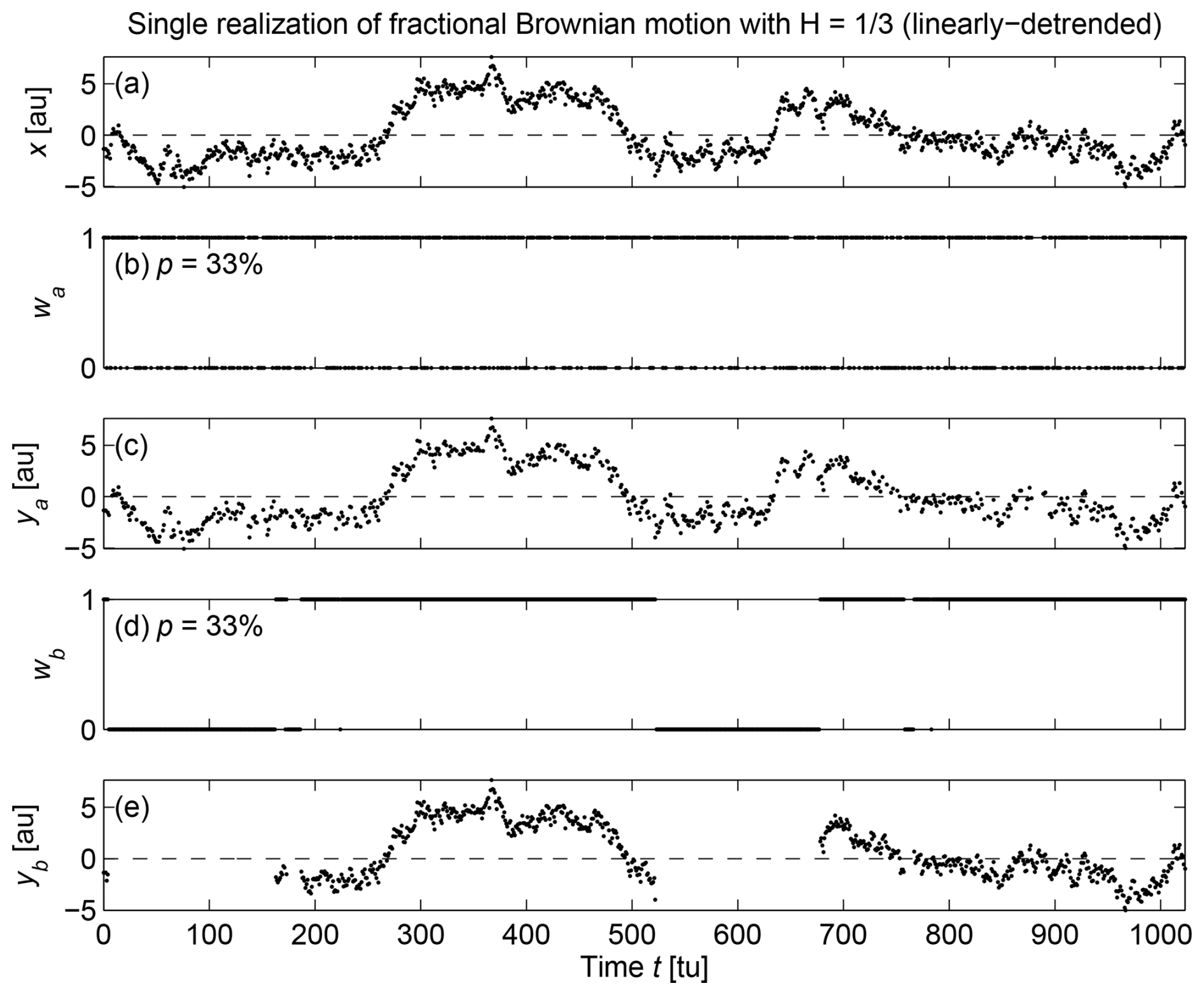
Figure 1 Example (one realization) for p=33 % missing samples of (a) original fractional Brownian motion (with $H=\mathrm{1}/\mathrm{3}$) series x, (b) sampling function with Bernoulli missing samples w_a, (c) observed series y_a, (d) sampling function with batch-Bernoulli missing samples w_b, and (e) observed series y_b. For better visualization, missing samples are not shown in (c) and (e), rather than being set to zero.

3 Applications

3.1 Fractional Brownian motion synthetic data

To illustrate the effects of missing samples on PSD estimation, we first generate synthetic random data using Matlab's wfbm function, which generates fractional Brownian motion signals for a given Hurst parameter H ($\mathrm{0}<H<\mathrm{1}$) and length N, following the algorithm proposed by Abry and Sellan (1996). Although the fractional Brownian motion is not a stationary random process, its spectral density exists for $\mathrm{0}<H\le \mathrm{1}/\mathrm{2}$ and is proportional to $f_k^{-(\mathrm{2}H+\mathrm{1})}$, which corresponds to the limit of the periodogram estimate when N→∞ (Kuleshov and Grudin, 2013). We test two values of the Hurst parameter, $H=\mathrm{1}/\mathrm{3}$, which gives a spectral slope $-(\mathrm{2}H+\mathrm{1})=-\mathrm{5}/\mathrm{3}$, and $H=\mathrm{1}/\mathrm{2}$, which gives a spectral slope $-(\mathrm{2}H+\mathrm{1})=-\mathrm{2}$. The first slope value is chosen to illustrate the case of isotropic homogeneous turbulence in the inertial range, if the frequency f represents the wavenumber (Kolmogorov, 1941; Obukhov, 1941, 1949; Corrsin, 1951). The second slope value is chosen to illustrate the case of discontinuities associated with, e.g. atmospheric or oceanic fronts (Boyd, 1992). For each value of H, we generate M series of N samples, and the expected value operator E is approximated by the arithmetic average over the M realizations. Here, we chose N=2¹⁰ (yielding almost three decades in frequency) and M=10⁴. Each series were linearly-detrended using the Matlab function detrend. An example of a linearly-detrended series for $H=\mathrm{1}/\mathrm{3}$ is shown in Fig. 1a.

3.1.1 Effects of autocorrelation function estimator

The autocorrelation functions of x for $H=\mathrm{1}/\mathrm{3}$ estimated by the different estimators are shown in Fig. 2a. Equation (A14) is illustrated in Fig. 2b for real-valued series.

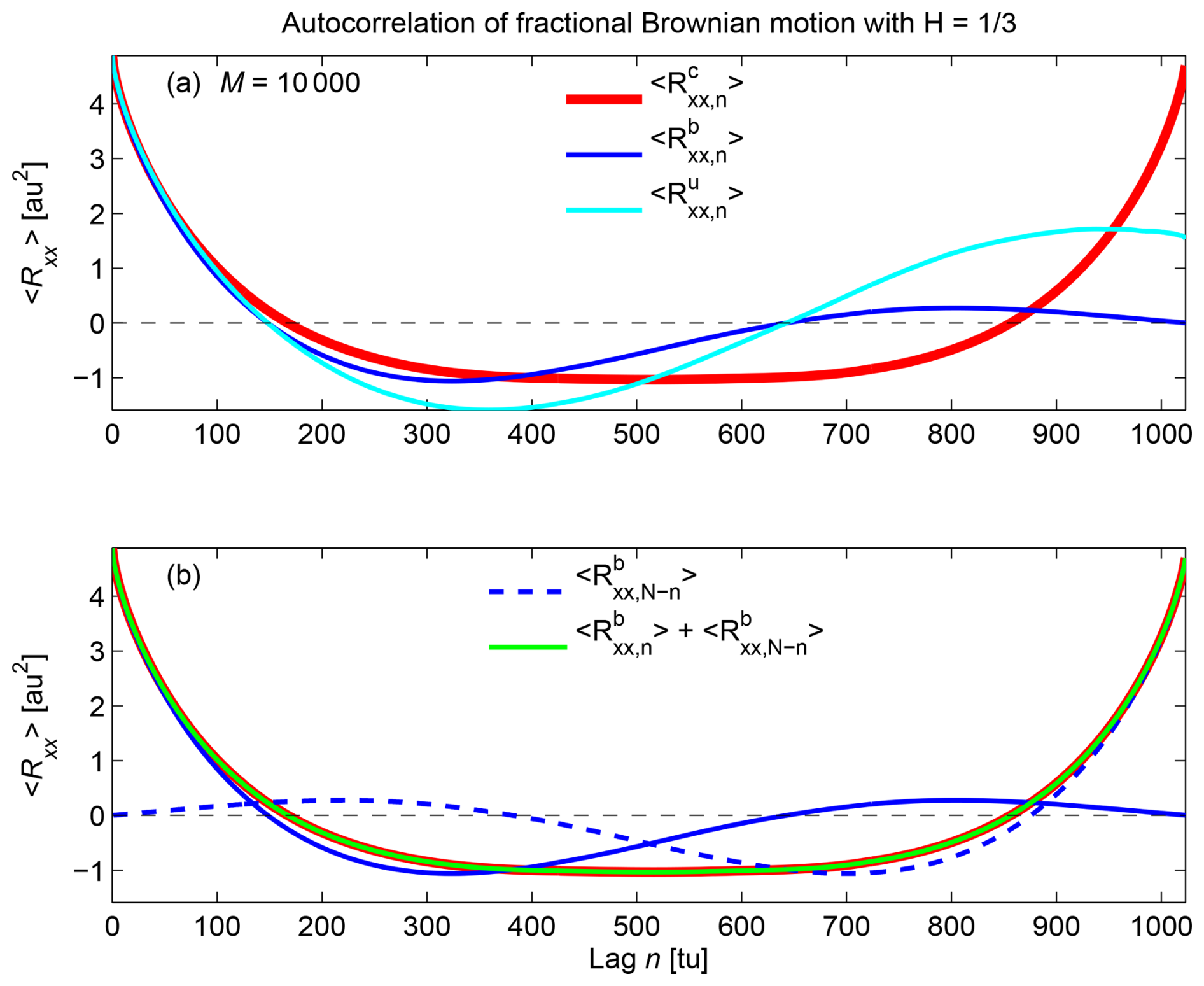
Figure 2 (a) Estimates (averaged over M=10⁴ realizations) of circular unbiased autocorrelation $R_{xx,n}^{\mathrm{c}}$ (red), standard biased autocorrelation $R_{xx,n}^{\mathrm{b}}$ (blue), and standard unbiased autocorrelation $R_{xx,n}^{\mathrm{u}}$ (cyan). Equation (A14) is illustrated in (b), where the flipped standard biased autocorrelation $R_{xx,N-n}^{\mathrm{b}}$ (dashed blue) and the sum $R_{xx,n}^{\mathrm{b}}+R_{xx,N-n}^{\mathrm{b}}$ (green) are also shown.

The PSD of x for $H=\mathrm{1}/\mathrm{3}$ and $H=\mathrm{1}/\mathrm{2}$ estimated by the different estimators are shown in Fig. 3. With no missing sample, all estimators recover the theoretical spectral slopes over most of the frequency domain for both $H=\mathrm{1}/\mathrm{3}$ and $H=\mathrm{1}/\mathrm{2}$, but $S_{xx}^{\mathrm{u}}$ is noisier than the other estimators, especially at high frequencies, even when averaged over M=10⁴ realizations.

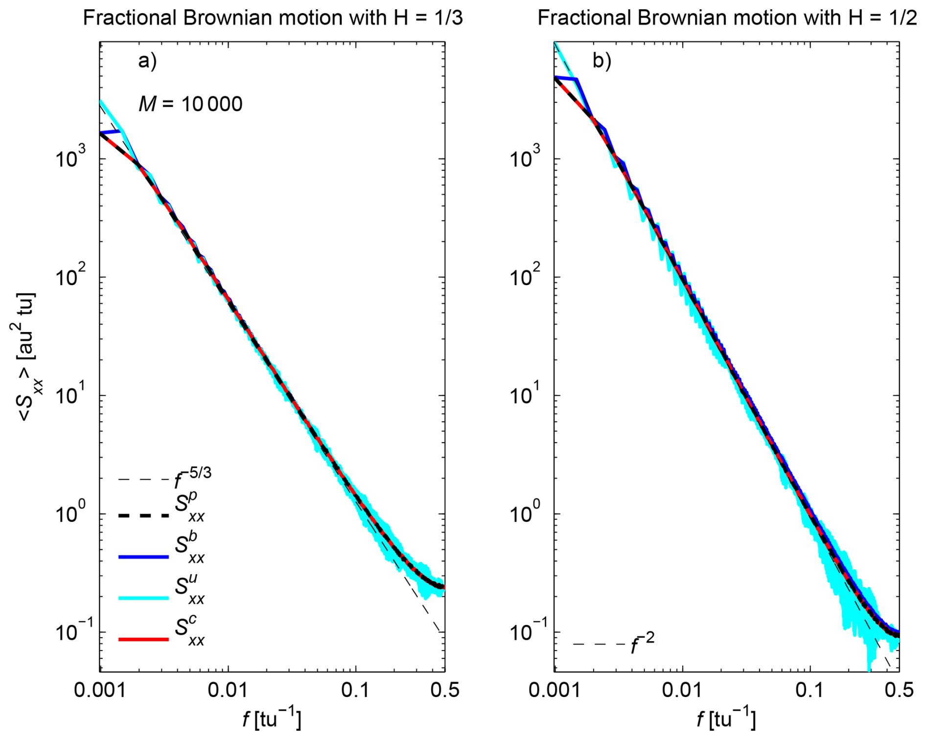
Figure 3 PSD estimates (averaged over M=10⁴ realizations) of fractional Brownian motion for (a) $H=\mathrm{1}/\mathrm{3}$ and (b) $H=\mathrm{1}/\mathrm{2}$, estimated by $S_{xx}^{\mathrm{p}}$ (thick black), $S_{xx}^{\mathrm{b}}$ (blue), $S_{xx}^{\mathrm{u}}$ (cyan), and $S_{xx}^{\mathrm{c}}$ (red). The theoretical spectral slopes are shown for reference (dashed black).

3.1.2 Effects of missing samples

We now turn to illustrate the effects of missing samples on PSD estimation. For each of the M series, we generate two sets of sampling functions, w_a with randomly missing samples occurring independently from each other (Fig. 1b) and w_b with batches of consecutively missed samples of randomly varying lengths (Fig. 1d). The number of missing samples N^′ is set to p percent of N for both sampling functions. In order for N^′ to maintain the same value for each realization of w_a and w_b, they are generated as follows. For w_a, initially set to $w_{a,n}=\mathrm{1}$, n=1, …, N, we generate N^′ values j_n, n=1, …, N^′, comprised between 2 and N−1 (to ensure that there are available samples at the beginning and end of the time series), sampled uniformly at random, without replacement, using the Matlab function randsample, and set $w_{a,j_n}=\mathrm{0}$, n=1, …, N^′. For w_b, we sequentially generate a series of lengths of batches of missing samples by generating a first length $L_{\mathrm{1}}^m$, randomly taken between 1 and N^′ using randsample, then a second length $L_{\mathrm{2}}^m$, randomly taken between 1 and $N^{\prime }-L_{\mathrm{1}}^m$, and so on until $\sum _{n=\mathrm{1}}^{N_L}{L}_n^m=N^{\prime }$, where N_L is the number of batches of missing samples. The series $L_n^m$, n=1, …, N_L, is then randomly reordered using the Matlab function randperm. We also generate a series of lengths of batches of available samples, $L_n^a$, n=1, …, N_L+1 (to ensure that there are available samples at the beginning and end of the time series) with a similar procedure, such that $\sum _{n=\mathrm{1}}^{N_L+\mathrm{1}}{L}_n^a=N-N^{\prime }$. Finally, we interspace available and missing samples with their respective batch lengths as follows: $w_{b,n}=\mathrm{1}$, n=1, …, $L_{\mathrm{1}}^a$, $w_{b,n}=\mathrm{0}$, $n=L_{\mathrm{1}}^a+\mathrm{1}$, …, $L_{\mathrm{1}}^a+L_{\mathrm{1}}^m$, etc. w_a is called a Bernoulli missing mechanism and is an example of missing completely at random (MCAR), while w_b is called a batch-Bernoulli missing mechanism and is an example of missing at random (MAR) (Rubin, 1976; Efromovich, 2018; Little and Rubin, 2019).

In this section, we set p=33 %. The resulting observed series (with missing samples not shown instead of replaced by zeros) are shown in Fig. 1c and e. PSD of the sampling functions are computed using Eq. (8) and averaged over the M realizations, showing that w_a has a white spectrum while w_b has a red spectrum (Fig. 4).

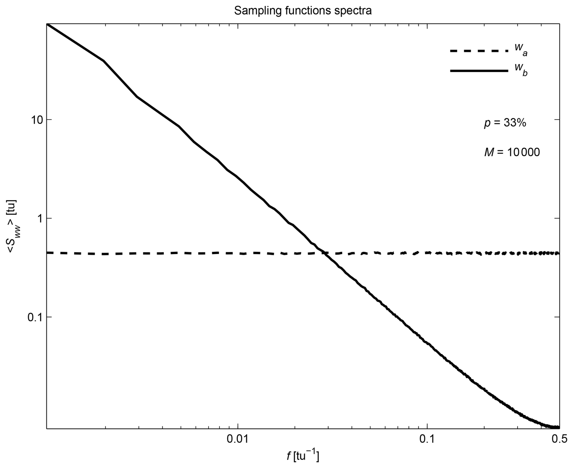
Figure 4 PSD (averaged over M=10⁴ realizations) of the sampling functions w_a (dashed line) and w_b (solid line) for p=33 % missing samples.

PSD of the observed series are computed using the different estimators presented in Sect. 2.3 and averaged over the M realizations. Spectra for $H=\mathrm{1}/\mathrm{3}$ are shown in Fig. 5. For both missing data schemes, both $S_{xx}^{\mathrm{u}}$ and $S_{xx}^{\mathrm{c}}$ recover the $-\mathrm{5}/\mathrm{3}$ spectral slope over most of the frequency range, but these estimates get noisy at high frequencies, even when averaged over M=10⁴ realizations, especially for $S_{xx}^{\mathrm{u}}$. $S_{xx}^{\mathrm{b}}$ and $S_{xx}^{\mathrm{L}}$ perform similarly, with a slightly biased spectral slope for w_b and PSD leveling at high frequencies for w_a. In contrast, $S_{xx}^{\mathrm{G}}$ is strongly biased for both missing data schemes.

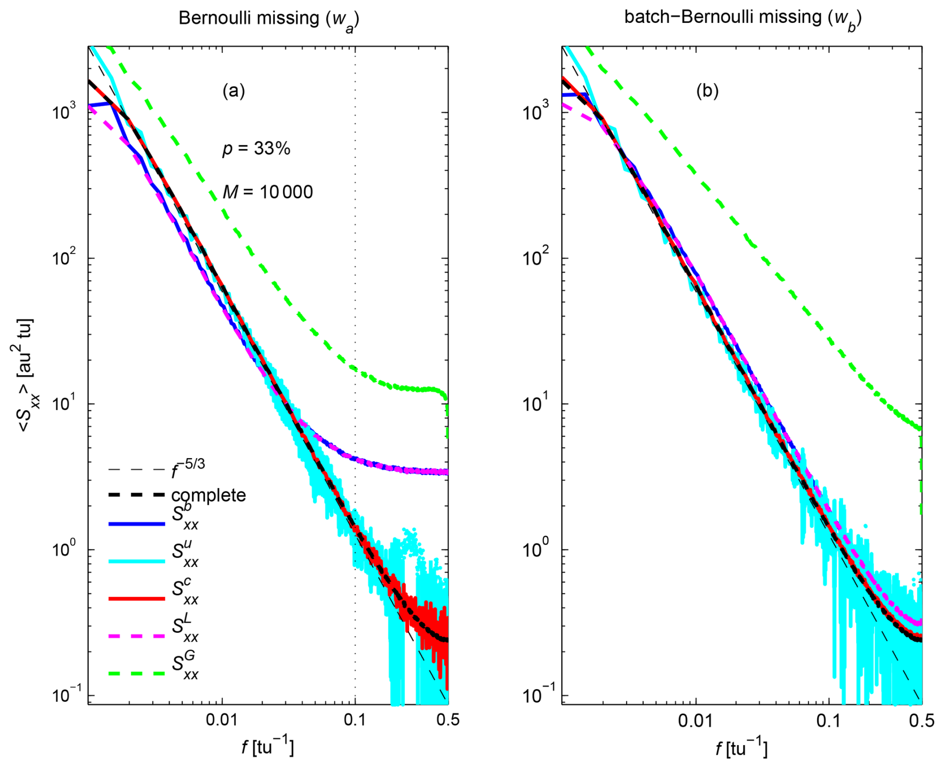
Figure 5 PSD (averaged over M=10⁴ realizations) of the complete (without missing samples) fractional Brownian motion with $H=\mathrm{1}/\mathrm{3}$ (thick black), and of the observed series with missing samples using $S_{xx}^{\mathrm{b}}$ (blue), $S_{xx}^{\mathrm{u}}$ (cyan), $S_{xx}^{\mathrm{c}}$ (red), $S_{xx}^{\mathrm{L}}$ (magenta), and $S_{xx}^{\mathrm{G}}$ (green) for the sampling functions (a) w_a and (b) w_b with p=33 % missing samples. The theoretical spectral slope is shown for reference (dashed black). The vertical dotted line in (a) indicates the frequency (f=0.1) at which the PSD histograms are shown in Fig. 6.

The unbiasedness of $S_{xx}^{\mathrm{u}}$ and $S_{xx}^{\mathrm{c}}$ comes with an increased variance of the estimator (Jones, 1962) and potential negative values at some frequencies (Jones, 1971), as illustrated in Fig. 6 for f=0.1. Although PSD are always positive for $S_{xx}^{\mathrm{b}}$, $S_{xx}^{\mathrm{L}}$, and $S_{xx}^{\mathrm{G}}$, the average values of these estimates are biased relative to the value obtained without missing samples. In contrast, negative values can be obtained with $S_{xx}^{\mathrm{u}}$ and $S_{xx}^{\mathrm{c}}$, but the average values of these estimates are close to the value obtained without missing samples. $S_{xx}^{\mathrm{u}}$ has the largest variance among all estimators tested.

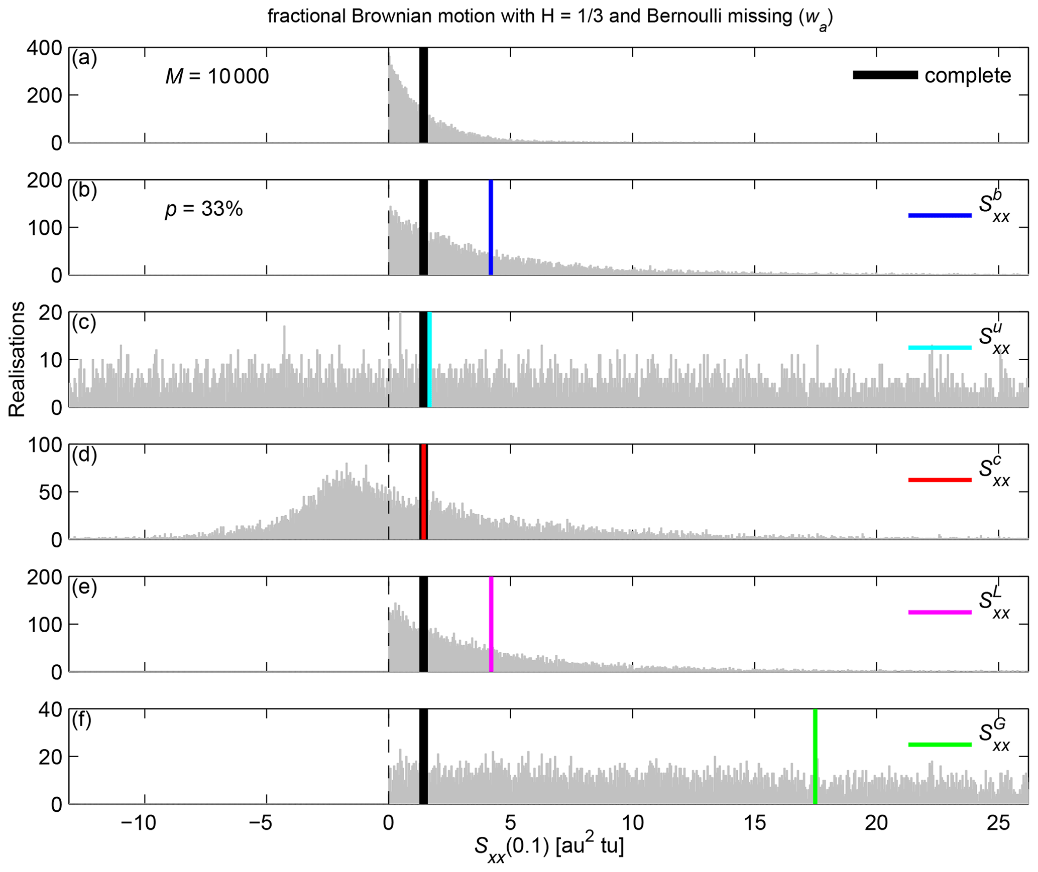
Figure 6 Histograms of M=10⁴ PSD estimates at a particular frequency (f=0.1) of (a) the complete (without missing samples) fractional Brownian motion with $H=\mathrm{1}/\mathrm{3}$, and of the observed series with p=33 % Bernoulli missing samples using (b) $S_{xx}^{\mathrm{b}}$, (c) $S_{xx}^{\mathrm{u}}$, (d) $S_{xx}^{\mathrm{c}}$, (e) $S_{xx}^{\mathrm{L}}$, and (f) $S_{xx}^{\mathrm{G}}$. Vertical solid lines show the average values.

Although negative PSD values are not physically meaningful and may appear to be an undesirable feature of the unbiased estimators, they are necessary for the unbiasedness of the estimators. Indeed, if one uses the absolute value of Eq. (13) to convert negative values into positive values (Fig. 6f), as proposed by Gao et al. (2021), the resulting average PSD (Fig. 5, green) are even more biased than those obtained with classical estimators such as $S_{xx}^{\mathrm{b}}$ and $S_{xx}^{\mathrm{L}}$.

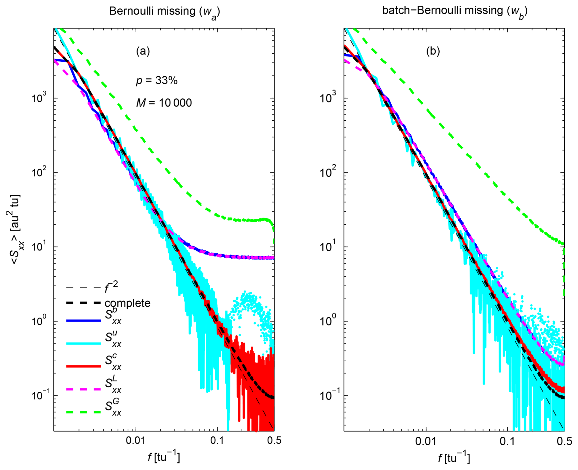
To investigate the sensitivity of the different estimators to the spectral slope, Fig. 7 shows the different estimated PSD for fractional Brownian motion with $H=\mathrm{1}/\mathrm{2}$. The results are very similar to the case of $H=\mathrm{1}/\mathrm{3}$ (Fig. 5), except that both unbiased estimators $S_{xx}^{\mathrm{u}}$ and $S_{xx}^{\mathrm{c}}$ are even noisier at high frequencies. Of course, noise could be reduced by increasing M, but in practice the number of independent realizations available is usually limited. Further averaging can be performed by averaging PSD estimates within larger frequency bins (i.e., band-averaging). This is illustrated using laboratory turbulence data in the next section.

Figure 7 Same as Fig. 5 for fractional Brownian motion with $H=\mathrm{1}/\mathrm{2}$.

3.2 Case study: decaying turbulence in an active grid-generated air flow

We now turn to an example involving actual data: air flow velocities measured downstream of an active turbulence-generating grid in the return-type Corrsin wind tunnel experiment reported by Kang et al. (2003). The Reynolds number is Re_λ≈720. Velocities were measured using an X-wire probe at a sampling rate of 40 kHz mounted at a downstream distance of 20 L, where L=0.152 m is the mesh size of the grid. Following Kang et al. (2003), the 15 min duration velocity record was divided into M=2195 segments (with 50 % overlap) of N=2¹⁵ samples each. Velocity records for each segment were linearly-detrended using the Matlab function detrend. While Kang et al. (2003) multiplied each segment by a Bartlett window prior to estimating PSD, here, following Damaschke et al. (2024), we do not apply any window so as to obtain asymptotically-unbiased estimates. The original record is complete (no missing sample), and the PSD of the streamwise velocity component is estimated using the periodogram estimator $S_{xx}^{\mathrm{p}}$, averaged over the M=2195 realizations (Fig. 8, thick black). The spectrum is very similar to that shown in Fig. 3 of Kang et al. (2003), with a spectral slope close to $-\mathrm{5}/\mathrm{3}$ over two decades (10 s${}^{-\mathrm{1}}<f<{\mathrm{10}}^{\mathrm{3}}$ s⁻¹).

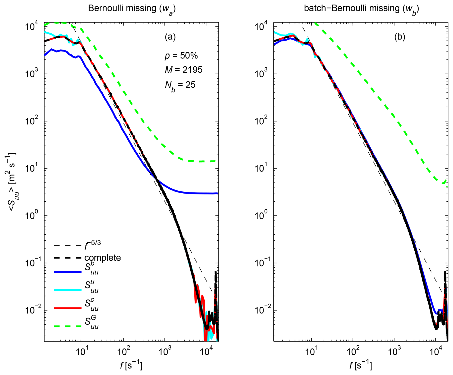
Figure 8 Same as Fig. 5 for decaying turbulence in an active grid-generated air flow from Kang et al. (2003), with p=50 % missing samples. Spectra for data with missing samples have been band-averaged over N_b=25 frequency bins per decade.

To investigate the effects of missing samples on PSD estimation, we generate Bernoulli and batch-Bernoulli sampling functions w_a and w_b, respectively, with the same algorithm used in the previous section. Here, we test the more stringent case of p=50 % missing samples, a large value beyond which time series are usually considered unusable for conventional spectral analysis. Due to the larger fraction of missing samples and the smaller number of realizations than in the previous section, the spectral estimates obtained with $S_{xx}^{\mathrm{u}}$ and $S_{xx}^{\mathrm{c}}$ are very noisy (not shown). Therefore, we further averaged all spectral estimates by band-averaging over N_b=25 frequency bins per decade (Fig. 8). With band-averaging, $S_{xx}^{\mathrm{u}}$ and $S_{xx}^{\mathrm{c}}$ have similar performances and recover the $-\mathrm{5}/\mathrm{3}$ spectral slope over the two decades. In contrast, $S_{xx}^{\mathrm{G}}$ is strongly biased for both missing data schemes, while $S_{xx}^{\mathrm{b}}$ is biased only for the Bernoulli missing data scheme. $S_{xx}^{\mathrm{L}}$ is not shown because it would have to be multiplied by a factor of 2×10⁴ to be comparable to the PSD without missing sample, and would then be very similar to $S_{xx}^{\mathrm{b}}$.

4 Discussion and conclusions

Wiener–Khinchin's theorem for finite discrete data states that the periodogram estimator (Eq. 8) is the finite discrete Fourier transform of the circular estimator of the autocorrelation function of the signal $R_{xx}^{\mathrm{c}}$ (Eq. 9), while the finite discrete Fourier transform of the standard biased estimator of the autocorrelation function $R_{xx}^{\mathrm{b}}$ (Eq. 11), usually considered in the literature (e.g Stoica and Moses, 2005), yields spectral estimates with twice the frequency resolution of the periodogram estimator. Since $R_{xx}^{\mathrm{b}}$ is a biased estimator of the autocorrelation function, the standard unbiased estimator $R_{xx}^{\mathrm{u}}$ is sometimes used to estimate the PSD (Eq. 13). This is the estimator commonly used to estimate the PSD of a signal with missing samples, as first proposed by Jones (1962). Here, we instead propose using the unbiased estimator $R_{xx}^{\mathrm{c}}$, since the number of data pairs available for each lag (N_n) is always greater or equal to the number (M_n) available for $R_{xx}^{\mathrm{u}}$, which decreases the variance of the PSD estimator. Furthermore, computing $R_{xx}^{\mathrm{c}}$ using the fast Fourier transform algorithm requires half the memory usage necessary for computing $R_{xx}^{\mathrm{u}}$.

The effects of missing samples on the PSD estimation are illustrated in Sect. 3.1 using fractional Brownian motion synthetic data with Hurst parameters $H=\mathrm{1}/\mathrm{3}$ and $H=\mathrm{1}/\mathrm{2}$, with constant power spectral slopes in log-log space of $-\mathrm{5}/\mathrm{3}$ and −2, respectively, along with synthetic Bernoulli (missing completely at random) and batch-Bernoulli (missing at random) sampling functions with p=33 % missing samples. The results show that the standard estimator $S_{xx}^{\mathrm{b}}$, as well as the commonly-used Lomb-Scargle estimator $S_{xx}^{\mathrm{L}}$, are biased and do not recover the original spectral slopes throughout the frequency range. In contrast, $S_{xx}^{\mathrm{u}}$ and $S_{xx}^{\mathrm{c}}$ are unbiased and recover the original spectral slopes throughout the frequency range, but they have a much larger variance than the biased estimators, especially for $S_{xx}^{\mathrm{u}}$, with possible negative values for individual realizations. Although this may be seen as an undesirable property of these estimators, we show that this is actually a necessary feature to obtain unbiased estimates. Indeed, trying to eliminate the negative values by taking their absolute value (as, e.g., Gao et al., 2021, did) leads to strongly biased estimates and distorted spectral slopes.

Similar results are obtained using actual data from a laboratory experiment of decaying turbulence in an active grid-generated air flow (Kang et al., 2003), along with synthetic Bernoulli and batch-Bernoulli sampling functions with p=50 % missing samples. To reduce the high level of noise of $S_{xx}^{\mathrm{u}}$ and $S_{xx}^{\mathrm{c}}$, all spectral estimates were further band-averaged over 25 frequency bins per decade. With band-averaging, $S_{xx}^{\mathrm{u}}$ and $S_{xx}^{\mathrm{c}}$ have similar performances and recover the $-\mathrm{5}/\mathrm{3}$ spectral slope over the same frequency range as for the original data, while the other estimators remain biased.

To obtain an unbiased PSD estimator, Damaschke et al. (2024) propose a combination of three methods, the first using $S_{xx}^{\mathrm{u}}$, the second restricting the domain of the autocorrelation function (maximum lag much smaller than N−1) to reduce the variance of the spectral estimates, and the third correcting the autocorrelation estimate after removal of the estimated mean value of the signal. Their first method is almost the same as that proposed here, except that we use $S_{xx}^{\mathrm{c}}$ instead of $S_{xx}^{\mathrm{u}}$. Their second method is similar to that proposed by Efromovich (2014) and provides unbiased PSD estimates for random processes with finite memory, for which the autocorrelation function becomes zero at lags beyond the memory length, provided the maximum lag considered is equal to or longer than the memory length. Here, our synthetic data do not have finite memory, as the autocorrelation function $S_{xx}^{\mathrm{u}}$ does not tend to zero for large lags (Fig. 2a). Since actual processes do not necessarily have finite memory, as in the turbulence data considered in Sect. 3.2, we do not restrict the domain of the autocorrelation function, accepting the large variance of the resulting PSD estimates. Finally, since actual processes also do not necessarily have zero mean value, the correction proposed by Damaschke et al. (2024) should be used to obtain strictly unbiased PSD estimates. However, even without applying their correction, the PSD estimator proposed here is asymptotically unbiased as N→∞, so the correction proposed by Damaschke et al. (2024) becomes unnecessary for long time series, such as those considered here (N≥2¹⁰).

As with the periodogram estimator $S_{xx}^{\mathrm{p}}$, one problem with $S_{xx}^{\mathrm{c}}$ is that it assumes that the observed process is periodic with period T=NΔt. However, this is rarely the case for actual processes, including those considered here, and the lack of periodicity leads to spectral leakage of signal frequencies different from the resolvable Fourier frequencies, which contaminates the estimated PSD. For the sake of obtaining asymptotically-unbiased estimates, this problem has been ignored here. Spectral leakage can be reduced by windowing the time series prior to estimating PSD (e.g., Stoica and Moses, 2005) with any of the proposed estimators.

Appendix A: The Wiener–Khinchin theorem for finite discrete data

Consider a time series of N samples {x_n}, n=0, …, N−1, sampled at equally spaced time intervals Δt from an infinite, continuous, and stationary random process x(t), such that x_n=x(nΔt), spanning the time period T=NΔt. Its discrete finite Fourier transform is defined by

$$\begin{array}{}\text{(A1)}& X_k=\sum _{n=\mathrm{0}}^{N-\mathrm{1}}{x}_n{e}^{-i\mathrm{2}\mathit{\pi }\frac{k}{N}n}\mathrm{\Delta }tk=\mathrm{0},\mathrm{\dots },N-\mathrm{1},\end{array}$$

at discrete Fourier frequencies

$$\begin{array}{}\text{(A2)}& f_k={\displaystyle \frac{k}{T}}.\end{array}$$

The periodogram estimator of the auto-spectral density of x is defined by (Stoica and Moses, 2005)

$$\begin{array}{}\text{(A3)}& S_{xx,k}={\displaystyle \frac{\mathrm{1}}{T}}{X}_k{X}_k^{*}.\end{array}$$

Using Eq. (A1), Eq. (A3) becomes

$$\begin{array}{}\text{(A4)}& S_{xx,k}={\displaystyle \frac{\mathrm{\Delta }t}{N}}\sum _{n=\mathrm{0}}^{N-\mathrm{1}}\sum _{m=\mathrm{0}}^{N-\mathrm{1}}{x}_n{x}_m^{*}{e}^{-i\mathrm{2}\mathit{\pi }\frac{k}{N}(n-m)}.\end{array}$$

Let $n^{\prime }=n-m$ replace the variable n in Eq. (A4). The summation limits for n^′ are $n^{\prime }=-m$ when n=0, and $n^{\prime }=N-\mathrm{1}-m$ when $n=N-\mathrm{1}$, modifying the summation domain as illustrated in Fig. A1. Then, Eq. (A4) becomes

$$\begin{array}{}\text{(A5)}& \begin{array}{rl}{S}_{xx,k}& ={\displaystyle \frac{\mathrm{\Delta }t}{N}}\left(\sum _{n^{\prime }=-(N-\mathrm{1})}^{-\mathrm{1}}\sum _{m=-n^{\prime }}^{N-\mathrm{1}}{x}_{m+n^{\prime }}{x}_m^{*}{e}^{-i\mathrm{2}\mathit{\pi }\frac{k}{N}{n}^{\prime }}\right.\\ & \left.+\sum _{n^{\prime }=\mathrm{0}}^{N-\mathrm{1}}\sum _{m=\mathrm{0}}^{N-\mathrm{1}-n^{\prime }}{x}_{m+n^{\prime }}{x}_m^{*}{e}^{-i\mathrm{2}\mathit{\pi }\frac{k}{N}{n}^{\prime }}\right).\end{array}\end{array}$$

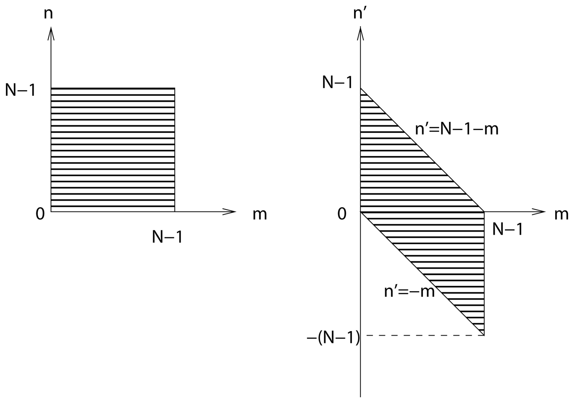
Figure A1 Change of variables for the derivation of the Wiener–Khinchin theorem (adapted from Bendat and Piersol, 2011).

Defining the standard biased estimator of the auto-correlation function of x as follows (Stoica and Moses, 2005)

$$\begin{array}{}\text{(A6)}& R_{xx,n^{\prime }}^{\mathrm{b}}=\left\{\begin{array}{ll}\frac{\mathrm{1}}{N}\sum _{m=\mathrm{0}}^{N-\mathrm{1}-n^{\prime }}{x}_{m+n^{\prime }}{x}_m^{*}& \mathrm{if}{n}^{\prime }\ge \mathrm{0},\\ \frac{\mathrm{1}}{N}\sum _{m=-n^{\prime }}^{N-\mathrm{1}}{x}_{m+n^{\prime }}{x}_m^{*}& \mathrm{if}{n}^{\prime }<\mathrm{0},\end{array}\right.\end{array}$$

Eq. (A5) becomes

$$\begin{array}{}\text{(A7)}& S_{xx,k}=\sum _{n^{\prime }=-(N-\mathrm{1})}^{N-\mathrm{1}}{R}_{xx,n^{\prime }}^{\mathrm{b}}{e}^{-i\mathrm{2}\mathit{\pi }\frac{k}{N}{n}^{\prime }}\mathrm{\Delta }tk=\mathrm{0},\mathrm{\dots },N-\mathrm{1}.\end{array}$$

$R_{xx,n^{\prime }}^{\mathrm{b}}$ is a biased estimator, since its expected value is

$$\begin{array}{}\text{(A8)}& E\left[R_{xx,n^{\prime }}^{\mathrm{b}}\right]={\displaystyle \frac{N-\left|n^{\prime }\right|}{N}}{R}_{xx}\left(n^{\prime }\mathrm{\Delta }t\right).\end{array}$$

An unbiased estimator, called the standard unbiased estimator of the autocorrelation function of x (Stoica and Moses, 2005), can therefore be defined by

$$\begin{array}{}\text{(A9)}& R_{xx,n^{\prime }}^{\mathrm{u}}={\displaystyle \frac{N}{N-\left|n^{\prime }\right|}}{R}_{xx,n^{\prime }}^{\mathrm{b}}.\end{array}$$

The right-hand side of Eq. (A7) looks like the finite Fourier transform of $R_{xx}^{\mathrm{b}}$, but the summation is carried over 2N−1 rather than N samples as in Eq. (A1). Consequently, the finite Fourier transform of $R_{xx}^{\mathrm{b}}$ yields 2N−1 Fourier frequencies $f_k=\frac{k}{\mathrm{2}T-\mathrm{\Delta }t}$, $k=-(N-\mathrm{1})$, …, N−1.

To estimate the auto-spectral density of x at the same Fourier frequencies as in Eq. (A2), let $n=n^{\prime }+N$ replace n^′ for $n^{\prime }<\mathrm{0}$ and $n=n^{\prime }$ replace n^′ for $n^{\prime }\ge \mathrm{0}$ in Eq. (A5), which becomes

$$\begin{array}{}\text{(A10)}& \begin{array}{rl}{S}_{xx,k}& ={\displaystyle \frac{\mathrm{\Delta }t}{N}}\left(\sum _{n=\mathrm{1}}^{N-\mathrm{1}}\sum _{m=N-n}^{N-\mathrm{1}}{x}_{m+n-N}{x}_m^{*}{e}^{-i\mathrm{2}\mathit{\pi }\frac{k}{N}n}\right.\\ & \left.+\sum _{n=\mathrm{0}}^{N-\mathrm{1}}\sum _{m=\mathrm{0}}^{N-\mathrm{1}-n}{x}_{m+n}{x}_m^{*}{e}^{-i\mathrm{2}\mathit{\pi }\frac{k}{N}n}\right).\end{array}\end{array}$$

Defining the circular unbiased estimator of the autocorrelation function of x as follows (Bendat and Piersol, 2011)

$$\begin{array}{}\text{(A11)}& \begin{array}{rl}& R_{xx,n}^{\mathrm{c}}=\\ & \left\{\begin{array}{ll}\frac{\mathrm{1}}{N}\sum _{m=\mathrm{0}}^{N-\mathrm{1}}{x}_m{x}_m^{*}& \mathrm{for}n=\mathrm{0},\\ \frac{\mathrm{1}}{N}\left(\sum _{m=\mathrm{0}}^{N-\mathrm{1}-n}{x}_{m+n}{x}_m^{*}+\sum _{m=N-n}^{N-\mathrm{1}}{x}_{m+n-N}{x}_m^{*}\right)& \mathrm{for}n=\mathrm{1},\mathrm{\dots },N-\mathrm{1},\end{array}\right.\end{array}\end{array}$$

Eq. (A10) becomes

$$\begin{array}{}\text{(A12)}& S_{xx,k}=\sum _{n=\mathrm{0}}^{N-\mathrm{1}}{R}_{xx,n}^{\mathrm{c}}{e}^{-i\mathrm{2}\mathit{\pi }\frac{k}{N}n}\mathrm{\Delta }tk=\mathrm{0},\mathrm{\dots },N-\mathrm{1}.\end{array}$$

$R_{xx,n}^{\mathrm{c}}$ is an unbiased estimator, since the summations in Eq. (A11) are always carried over N data pairs, and therefore

$$\begin{array}{}\text{(A13)}& E\left[R_{xx,n}^{\mathrm{c}}\right]=R_{xx}\left(n\mathrm{\Delta }t\right).\end{array}$$

The Wiener–Khinchin theorem (Eq. A12) states that the periodogram estimator of the auto-spectral density of x is the finite Fourier transform of the circular unbiased estimator of the autocorrelation function of x. It is called circular because, when using the finite discrete Fourier transform, the time series x(t) is considered periodic of period T=NΔt, then $x_{m+n-N}=x_{m+n}$ so that the second part of the right-hand side of Eq. (A11) for n≥1 represents the remainder of the autocorrelation terms for indices that go beyond N−1, for which the beginning of the time series is used again (see Fig. 11.4 in Bendat and Piersol, 2011).

$R_{xx,n}^{\mathrm{c}}$ can also be expressed as

$$\begin{array}{}\text{(A14)}& R_{xx,n}^{\mathrm{c}}=R_{xx,n}^{\mathrm{b}}+R_{xx,N-n}^{\mathrm{b}*},\end{array}$$

or equivalently

$$\begin{array}{}\text{(A15)}& R_{xx,n}^{\mathrm{c}}={\displaystyle \frac{N-n}{N}}{R}_{xx,n}^{\mathrm{u}}+{\displaystyle \frac{n}{N}}{R}_{xx,N-n}^{\mathrm{u}*}.\end{array}$$

In the limit of infinitely long time series,

$$\begin{array}{}\text{(A16)}& \underset{N\to +\mathrm{\infty }}{lim}{R}_{xx,n}^{\mathrm{c}}=\underset{N\to +\mathrm{\infty }}{lim}{R}_{xx,n}^{\mathrm{u}}.\end{array}$$

Appendix B: Asymptotically-unbiased nonparametric estimation of the cross-spectral density from uniformly-spaced data with missing samples

The algorithm (implemented with Matlab) to obtain an asymptotically-unbiased estimate of the cross-spectral density of two stationary random processes from uniformly-spaced data with missing samples is detailed below.

Consider two series of N samples {x_n} and {y_n}, n=0,. …, N−1, sampled at equally spaced time (or distance) intervals Δt from two stationary random processes x(t) and y(t), such that x_n=x(nΔt) and y_n=y(nΔt), spanning the time period (or spatial length) T=NΔt. Suppose that the series have N_x<N and N_y<N missing values, respectively.

If the time series are not taken from random processes with zero mean values, an estimate of their mean values should be removed from the time series:

$$\begin{array}{ll}{\displaystyle }& {\displaystyle }x=x-\mathrm{nanmean}\left(x\right);\\ {\displaystyle }& {\displaystyle }y=y-\mathrm{nanmean}\left(y\right).\end{array}$$

Next, missing values should be replaced by zeros and sampling functions defined by

$$\begin{array}{}\text{(B1)}& w_{x,n}=\left\{\begin{array}{cl}\mathrm{1}& \mathrm{if}{x}_n\mathrm{is}\mathrm{recorded},\\ \mathrm{0}& \mathrm{otherwise},\end{array}\right.\end{array}$$

and

$$\begin{array}{}\text{(B2)}& w_{y,n}=\left\{\begin{array}{cl}\mathrm{1}& \mathrm{if}{y}_n\mathrm{is}\mathrm{recorded},\\ \mathrm{0}& \mathrm{otherwise},\end{array}\right.\end{array}$$

which is obtained by:

$$\begin{array}{ll}{\displaystyle }& {\displaystyle }\mathit{\%}\mathrm{replace}\mathrm{missing}\mathrm{samples}\mathrm{with}\mathrm{zeros}\\ {\displaystyle }& {\displaystyle }I=\mathrm{find}\left(\mathrm{isnan}\right(x\left)\right);\\ {\displaystyle }& {\displaystyle }x\left(I\right)=\mathrm{0};\\ {\displaystyle }& {\displaystyle }J=\mathrm{find}\left(\mathrm{isnan}\right(y\left)\right);\\ {\displaystyle }& {\displaystyle }y\left(J\right)=\mathrm{0};\\ {\displaystyle }& {\displaystyle }\mathit{\%}\mathrm{sampling}\mathrm{functions}\\ {\displaystyle }& {\displaystyle }wx=\mathrm{ones}\left(\mathrm{size}\right(x\left)\right);\\ {\displaystyle }& {\displaystyle }wx\left(I\right)=\mathrm{0};\\ {\displaystyle }& {\displaystyle }wy=\mathrm{ones}\left(\mathrm{size}\right(y\left)\right);\\ {\displaystyle }& {\displaystyle }wy\left(J\right)=\mathrm{0}.\end{array}$$

Generalizing Eq. (8), the discrete finite cross-spectral density of x and y is defined by

$$\begin{array}{}\text{(B3)}& S_{xy,k}^{\mathrm{b}}={\displaystyle \frac{\mathrm{1}}{T}}{X}_k{Y}_k^{*}k=\mathrm{0},\mathrm{\dots },N-\mathrm{1},\end{array}$$

where X and Y are the discrete finite Fourier transforms of x and y, respectively. With missing samples replaced with zeros, Eq. (B3) is a biased estimator of the cross-spectral density of x and y.

Generalizing the Wiener–Khinchin theorem (Eq. 9), the circular cross-correlation function of x and y is defined as the inverse Fourier transform of $S_{xy}^{\mathrm{b}}$:

$$\begin{array}{}\text{(B4)}& R_{xy,n}^{\mathrm{c},\mathrm{b}}=\sum _{k=\mathrm{0}}^{N-\mathrm{1}}{S}_{xy,k}^{\mathrm{b}}{e}^{i\mathrm{2}\mathit{\pi }\frac{k}{N}n}\mathrm{\Delta }tn=\mathrm{0},\mathrm{\dots },N-\mathrm{1}.\end{array}$$

With missing samples replaced with zeros, Eq. (B4) is a biased estimator of the circular cross-correlation function of x and y, and is obtained by:

$$Rb=\mathrm{ifft}\left(\mathrm{fft}\right(x).*\mathrm{conj}(\mathrm{fft}\left(y\right))/\mathrm{length}(x\left)\right).$$

Generalizing Eq. (18) using the Wiener–Khinchin theorem, the number of data pairs available to estimate the circular cross-correlation function of x and y is given by:

$$\begin{array}{}\text{(B5)}& N_{xy,n}=\sum _{k=\mathrm{0}}^{N-\mathrm{1}}{W}_{x,k}{W}_{y,k}^{*}{e}^{i\mathrm{2}\mathit{\pi }\frac{k}{N}n}\mathrm{\Delta }tn=\mathrm{0},\mathrm{\dots },N-\mathrm{1},\end{array}$$

where W_x and W_y are the discrete finite Fourier transforms of w_x and w_y, respectively. N_xy is obtained by:

$$\mathrm{Npairs}=\mathrm{round}\left(\mathrm{real}\right(\mathrm{ifft}\left(\mathrm{fft}\right(wx).*\mathrm{conj}(\mathrm{fft}\left(wy\right)\left)\right)\left)\right);$$

where the “round” and “real” operators are used to obtain real integer values for N_xy,n even with machine precision errors.

Then, the unbiased estimator of the circular cross-correlation function of x and y is defined by

$$\begin{array}{}\text{(B6)}& R_{xy,n}^{\mathrm{c},\mathrm{u}}={\displaystyle \frac{N}{N_{xy,n}}}{R}_{xy,n}^{\mathrm{c},\mathrm{b}}n=\mathrm{0},\mathrm{\dots },N-\mathrm{1}.\end{array}$$

If $N_{xy,n}=\mathrm{0}$, $R_{xy,n}^{\mathrm{c},\mathrm{u}}$ is set to zero. $R_{xy}^{\mathrm{c},\mathrm{u}}$ is obtained by:

$$\begin{array}{ll}{\displaystyle }& {\displaystyle }Ru=Rb*\mathrm{length}\left(x\right)./\mathrm{Npairs};\\ {\displaystyle }& {\displaystyle }\mathit{\%}\mathrm{if}\mathrm{no}\mathrm{data}\mathrm{pair}\mathrm{is}\mathrm{available}\mathrm{for}\mathrm{a}\mathrm{lag},\mathrm{set}Ru\mathrm{to}\mathrm{zero}\\ {\displaystyle }& {\displaystyle }Ru\left(\mathrm{find}\right(\mathrm{Npairs}==\mathrm{0}\left)\right)=\mathrm{0}.\end{array}$$

Finally, the unbiased estimator of the cross-spectral density of x and y is defined by

$$\begin{array}{}\text{(B7)}& S_{xy,k}^{\mathrm{u}}=\sum _{n=\mathrm{0}}^{N-\mathrm{1}}{R}_{xy,n}^{\mathrm{c},\mathrm{u}}{e}^{-i\mathrm{2}\mathit{\pi }\frac{k}{N}n}\mathrm{\Delta }tk=\mathrm{0},\mathrm{\dots },N-\mathrm{1},\end{array}$$

and is obtained by:

$$Su=\mathrm{fft}\left(Ru\right).$$