A machine learning approach to emulation and biophysical parameter estimation with the Community Land Model, version 5

Land models are essential tools for understanding and predicting terrestrial processes and climate–carbon feedbacks in the Earth system, but uncertainties in their future projections are poorly understood. Improvements in physical process realism and the representation of human influence arguably make models more comparable to reality but also increase the degrees of freedom in model configuration, leading to increased parametric uncertainty in projections. In this work we design and implement a machine learning approach to globally calibrate a subset of the parameters of the Community Land Model, version 5 (CLM5) to observations of carbon and water fluxes. We focus on parameters controlling biophysical features such as surface energy balance, hydrology, and carbon uptake. We first use parameter sensitivity simulations and a combination of objective metrics including ranked global mean sensitivity to multiple output variables and non-overlapping spatial pattern responses between parameters to narrow the parameter space and determine a subset of important CLM5 biophysical parameters for further analysis. Using a perturbed parameter ensemble, we then train a series of artificial feed-forward neural networks to emulate CLM5 output given parameter values as input. We use annual mean globally aggregated spatial variability in carbon and water fluxes as our emulation and calibration targets. Validation and out-of-sample tests are used to assess the predictive skill of the networks, and we utilize permutation feature importance and partial dependence methods to better interpret the results. The trained networks are then used to estimate global optimal parameter values with greater computational efficiency than achieved by hand tuning efforts and increased spatial scale relative to previous studies optimizing at a single site. By developing this methodology, our framework can help quantify the contribution of parameter uncertainty to overall uncertainty in land model projections.

1 Introduction

Land models were originally developed to provide lower boundary conditions for atmospheric general circulation models but have evolved to simulate important processes such as carbon cycling, ecosystem dynamics, terrestrial hydrology, and agriculture. Including these societally relevant processes helps provide insight into potential impacts on humans and ecosystems but also introduces additional sources of uncertainty in model predictions. This uncertainty is largely driven by a combination of insufficient observations and incomplete knowledge regarding mathematical representations of these processes. At the same time, adequately predicting terrestrial processes and climate–carbon feedbacks relies on improving these models and their predictive capabilities while minimizing sources of model error (Bonan and Doney, 2018).

For example, much of the uncertainty in projections of the terrestrial carbon cycle comes from differences in model parameterizations (Friedlingstein et al., 2006; Booth et al., 2012). Looking across 11 carbon-cycle climate models all forced by the same future climate scenario, Friedlingstein et al. (2014) found that not only was the magnitude of the land–atmosphere carbon flux different across models, but there was also disagreement in the sign, implying that the land could be either a net carbon sink or source by the end of the century. The model spread in predictions of land–atmosphere carbon fluxes was found to be strongly tied to process representation, such as model treatment of carbon dioxide fertilization and the nitrogen cycle. This situation has remained unchanged in the latest iteration of the Climate Model Intercomparison Project (CMIP6) (Arora et al., 2020).

There are several different sources of uncertainty in Earth system models. Variations in initial conditions produce internal variability uncertainty, mimicking internal climate processes including stochastic weather noise. Differences in imposed forcing through future scenarios or boundary conditions produce forcing uncertainty, representing the uncertainty in predicting the pathway of future carbon emissions. Inherent model uncertainty encompasses uncertainty in model structure and parameters and represents the various choices in how models use mathematical abstractions of physics, chemistry, and biology to represent processes within the Earth system. When contrasting land versus ocean carbon cycle uncertainty over time, Lovenduski and Bonan (2017) found that while uncertainty in the forcing dominates the ocean carbon cycle, the land carbon cycle is dominated by uncertainty in model structure and parameters.

Parametric uncertainty in land models has been traditionally explored through experimentation with different parameter values to test how variations impact resulting model predictions (e.g., Bauerle et al., 2014; Fischer et al., 2011; Göhler et al., 2013; Hawkins et al., 2019; Huo et al., 2019; Ricciuto et al., 2018; White et al., 2000; Zaehle et al., 2005). Hand tuning parameter values can be computationally inefficient, requiring many model simulations and large amounts of computer time, especially when the spatial domain is large or global. Single point simulations provide a lower computational cost and the ability to more easily run large ensembles; however, results from parameter estimation at a single site may not be transferable to other regions due to differences in climate, soil, and vegetation types (Post et al., 2017; Cai et al., 2019; Huang et al., 2016; Lu et al., 2018; Ray et al., 2015). Undirected model calibration can be limited in its ability to objectively assess whether the optimal parameter configuration has been found due to the ambiguous and subjective nature of the hand tuning process (Mendoza et al., 2015; Prihodko et al., 2008). A machine learning approach can help streamline this process by providing increased computational efficiency and reduced analysis time as well as objective methods to assess calibration results (Reichstein et al., 2019). Artificial feed-forward neural networks are a type of machine learning algorithm that can learn relationships between input and output data (Russell and Norvig, 1995; Hagan et al., 1996; Mitchell, 1997). By using neural networks to build a surrogate model that emulates the behavior of a land model, additional parameter values can be tested and optimized quickly and efficiently without running the full model, thus more effectively exploring the parameter space (Sanderson et al., 2008; Knutti et al., 2003).

In this work we seek to better understand land model uncertainty through variations in parameter choices. By exploring the CLM5 biophysical parameter space and determining sensitive parameters, we investigate the role that parameter choices play in overall model uncertainty. We first narrow the parameter space following a series of one-at-a-time sensitivity simulations assessed with objective metrics by ranking global mean sensitivity to multiple output variables and searching for low spatial pattern correlations between parameters. With a candidate list of important CLM5 biophysical parameters, we use model results from a perturbed parameter ensemble (PPE) to train a series of artificial feed-forward neural networks to emulate a subset of the outputs of CLM5. Here we utilize supervised learning, where the neural network is trained on known model parameter values and simulation output from the PPE. The networks are trained to predict annual mean spatial variability in carbon and water fluxes, given biophysical parameter values as input. The trained networks are then applied to globally estimate optimal parameter values with respect to observations, and these optimal values are tested with CLM5 to investigate changes in model predictive skill.

2 Model simulations and parameter selection

2.1 Community Land Model, version 5

For this work we use the latest version of the Community Land Model, CLM5 (Lawrence et al., 2019). We use the “satellite phenology” version of the model where vegetation distributions and leaf and stem area indices (LAI) are prescribed by remote sensing data (Bonan et al., 2002), thus reducing the degrees of freedom by turning off processes that in fully prognostic mode lead to the prediction of LAI. Vegetated land units in CLM are partitioned into up to 15 plant functional types (PFTs) plus bare ground. Some model parameter values (those associated with plant physiology) vary with PFT, an important consideration for this work. We select parameters associated with biogeophysical processes in CLM, such as surface energy fluxes, hydrology, and photosynthesis. Parametric uncertainty of biogeochemical processes in CLM5 (vegetation carbon and nitrogen cycling) under carbon dioxide and nitrogen fertilization scenarios were explored by Fisher et al. (2019), though that study did not include an optimization component.

We run the model globally with a horizontal resolution of 4^∘ in latitude and 5^∘ in longitude. This coarse resolution is intended to maximize computational efficiency and allow for a greater number of ensemble members in both the sensitivity simulations and the perturbed parameter ensemble. CLM is forced by the Global Soil Wetness Project, Phase 3 (GSWP3) meteorological forcing data, repeatedly sampled over the years 2000–2004. These years are chosen to provide a consistent 5-year period of present-day climate forcing for each simulation. GSWP3 is a reanalysis-based product providing 3-hourly precipitation, solar radiation, wind speed, humidity, downward longwave radiation, and bottom atmospheric layer temperature and pressure (http://hydro.iis.u-tokyo.ac.jp/GSWP3/, last access: October 2020). Each CLM simulation is run for 20 years, with the last 5 years used in the analysis. The first 15 years are used as spin-up to equilibrate the soil moisture and soil temperature (Fig. S1 in the Supplement). All simulations reach equilibrium after 15 years.

2.2 Parameter sensitivity simulations

We begin with a set of parameter sensitivity simulations to explore the effect of one-at-a-time parameter perturbations for 34 CLM5 biophysical parameters, the results of which will inform the selection of a narrowed list of key parameters to utilize in the emulation and optimization steps. Initial parameter selection of the 34 parameters is based on identifying tunable quantities in the model which are important for the calculation of biophysical processes, including evapotranspiration, photosynthesis, and soil hydrology. These 34 parameters include a mix of empirically derived parameters (10) and parameters that describe biophysical properties (24). Parameter ranges are based on an extensive literature review and expert judgment, utilizing observational evidence whenever possible (Tables S1 and S2 in the Supplement, and references therein). We run two model simulations for each parameter using the setup described above, one simulation using the minimum value of the parameter sensitivity range and one using the maximum value. Ten of the parameters vary with PFT and thus have PFT-specific sensitivity ranges that are applied in these simulations. In most cases, these PFT-varying parameters are uniformly perturbed across PFTs by the same perturbation amount relative to their default value (e.g., ±20 %). This approach accounts for the fact that the default values for a given parameter may vary across PFTs. For some parameters where the default values do not vary much across PFTs, all PFTs are perturbed to the same minimum or maximum value. Table S2 shows the details of the minimum and maximum values used for each parameter in the one-at-a-time sensitivity simulations, including the perturbation amounts for PFT-varying parameters.

We use seven different model outputs to assess the sensitivity of the 34 parameters. These outputs are gross primary production (GPP), evapotranspiration (ET), transpiration fraction (TF = transpiration / ET), sensible heat flux, soil moisture of the top 10 cm, total column soil moisture, and water table depth. These output fields are selected to span the relevant biogeophysical processes in the model. To narrow the parameter space and identify candidate parameters for further uncertainty quantification, we use multiple parameter selection criteria. First we assess the sensitivity of each parameter to the seven different outputs using a simple sensitivity metric. We call this the parameter effect (PE), detailed in Eq. (1), where $X_{p,max}$ and $X_{p,min}$ represent the model output of a quantity X from the simulations using the maximum and minimum values of parameter p, respectively. We calculate the 5-year annual mean PE at each grid point and then take the global mean of the resulting quantity.

$$\begin{array}{}\text{(1)}& \text{PE}\left(p\right)=\left|X_{p,max}-X_{p,min}\right|\end{array}$$

In order to account for differences in units between variables, the global mean PE values for each parameter are ranked across each output variable from highest to lowest, with the average of the individual ranks across all seven outputs used to assess overall sensitivity rank. The PE ranks for each parameter and output variable are shown in Table S3, along with the average and overall ranks. The annual mean PE for GPP for the final six parameters is shown in Fig. 1.

Figure 1 Annual mean parameter effect (PE) for GPP ($\mathrm{\mu }\mathrm{mol}{\mathrm{CO}}_{\mathrm{2}}{\mathrm{m}}^{-\mathrm{2}}{\mathrm{s}}^{-\mathrm{1}}$) for the final six parameters.

The second selection criterion uses spatial pattern correlations to maximize the sampled range of model physics and responses in the final parameter set. Filtering parameters by spatial pattern correlations helps avoid the situation where all the selected parameters control behavior in a certain region (e.g., the tropics but not at the mid or high latitudes). We compute this metric by calculating the spatial pattern correlation of the PE between all pairwise parameter combinations for each output. This method reveals parameters with similar spatial pattern responses and provides an additional means by which to narrow the parameter space. While one-at-a-time sensitivity studies do not explicitly account for parameter interactions (Rosolem et al., 2012), by calculating the spatial correlation between parameters and selecting those with low correlations, we indirectly account for some of these potential interactions.

Equation (2) details the pattern correlation calculation, where PC(p,q)_v is the spatial pattern correlation of the PE between parameters p and q for a given output variable v. The pairwise pattern correlations are then summed across the seven output variables (V=7). A visual representation of the sum of pattern correlations across outputs for each parameter combination is shown in Fig. S2. Then the average pattern correlation is calculated across parameters (Q=34), resulting in a single PC value for each parameter p. (This is equivalent to taking the average across rows or columns in Fig. S2.) The average pattern correlations are also ranked across parameters, though this time the ranks are computed from lowest to highest as we are looking for parameters which exhibit low spatial correlation between each other to sample the broadest possible space of model processes. The average pattern correlations and pattern correlation ranks for each parameter are shown in Table S4.

$$\begin{array}{}\text{(2)}& \text{PC}\left(p\right)={\displaystyle \frac{\mathrm{1}}{Q}}\sum _{q=\mathrm{1}}^Q\sum _{v=\mathrm{1}}^V\text{PC}(p,q{)}_v\end{array}$$

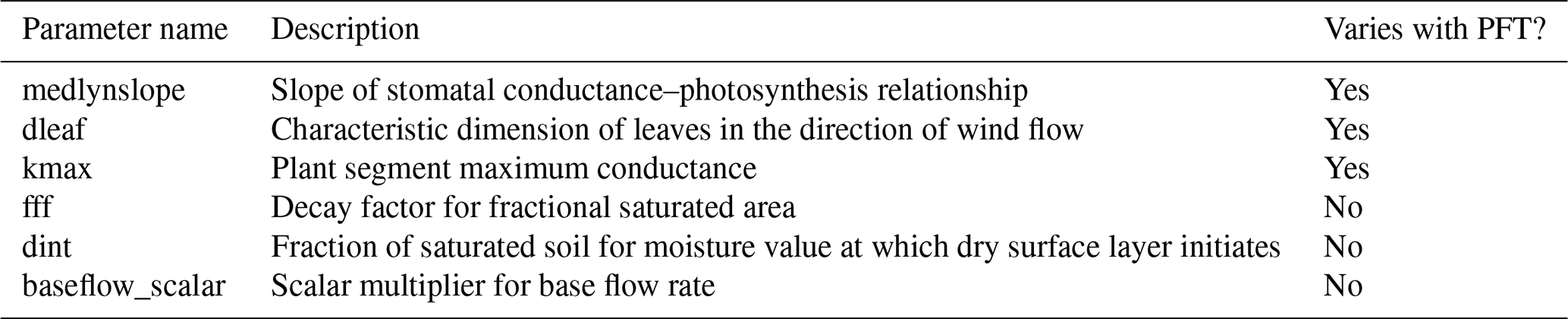
The pattern correlation ranks are averaged with the PE ranks to help inform the final list of candidate parameters (Table S5). We aim for a balance between parameters with high PE values across outputs and low spatial pattern correlations with other parameters. In this way we are selecting sensitive parameters in the model that do not all control the same behavior and looking across a range of outputs to inform this selection. We also prioritize parameters for which we are able to use observational data to better inform their uncertainty ranges, in particular for those parameters that vary with PFT. These results are detailed in Sect. 2.3. As a result of these parameter selection criteria, a list of 6 candidate parameters is chosen from the original set of 34. These six parameters, along with a short description of each, are shown in Table 1. A six-dimensional space was found during this study to be the practical limiting size for optimization, as we are motivated to include the most important parameters while also considering computational constraints. We first select the top four parameters by PE rank (medlynslope, kmax, fff, and dint). We then select dleaf because it has a relatively high parameter effect (PE rank =10) and because we are able to use observations to generate new PFT-specific uncertainty ranges for this parameter. All five of these parameters are among the top 50 % of parameters when looking by average rank across PE and PC ranks (Table S5). Finally, we select the parameter baseflow_scalar because it has the highest overall average rank, largely due to its low spatial pattern correlation with other parameters (PC rank =2). Additional information for these parameters, including their default CLM5 values, their uncertainty ranges, and references used to determine their minimum and maximum bounds, can be found in the tables in the Supplement.

Table 1 CLM5 candidate parameters selected based on sensitivity tests.

2.3 Using observations to inform PFT-specific parameter ranges

For some parameters that vary with PFT, we can improve estimates of plausible ranges by incorporating additional observational data. We can then define uncertainty ranges for a single parameter that vary in their bounds and widths across PFTs. The first parameter we constrain is dleaf, the characteristic dimension of leaves in the direction of wind flow. This parameter is relevant for boundary layer dynamics and relates to the structural form of the equation for leaf boundary layer resistance. The dleaf parameter has a constant fixed value across PFTs in the default CLM5 configuration but in the real world would likely vary by PFT. We use the TRY plant trait database (Kattge et al., 2011) to identify a dataset with concurrent measurements of leaf width and PFT-relevant information (e.g., leaf type, phenology, growth form). The TRY database included only one dataset with adequate leaf width measurements and enough information to associate the measurements with CLM PFTs. The particular dataset we use is from Northeast China (Prentice et al., 2011), which includes a total of 409 usable measurements of leaf width, each of which we assign to a CLM PFT. Some measurements are applied across multiple CLM PFTs based on the lack of biome variation in the dataset. Because we are utilizing measurements from one geographic location, we may not be adequately capturing biome variation (e.g., tropical versus temperate versus boreal PFTs), and this may impact the results. However, it is likely that this variation is small relative to other types of PFT variation (e.g., phenology) which we are able to capture using this dataset. Using the equations of Campbell and Norman (1998), which relate leaf width to dleaf by a leaf shape-dependent factor, we produce PFT-dependent uncertainty bounds for dleaf (Table S6). These minimum and maximum values are then applied consistently across all PFTs for the minimum and maximum dleaf perturbation simulations, respectively.

The second parameter we constrain using observational data is medlynslope, the slope of the stomatal conductance–photosynthesis relationship defined by Medlyn et al. (2011). This relationship is important for determining stomatal responses to environmental changes and calculating photosynthesis and transpiration. We use data from Lin et al. (2015) to perform a combination of genus- and species-based linear regressions of photosynthesis versus stomatal conductance to obtain slope values (Table S7). The minimum and maximum parameter values are taken from the set of slopes for each PFT. The only PFT we cannot constrain using this method is C3 Arctic grasses, due to a lack of available data. In this case we use a ±10 % perturbation from the default medlynslope value for C3 Arctic grasses. As with dleaf, the minimum and maximum values are then applied simultaneously across all PFTs for the minimum and maximum medlynslope perturbation simulations.

2.4 Perturbed parameter ensemble

To generate the parameter values for a perturbed parameter ensemble, we use Latin hypercube (LHC) (Mckay et al., 2000) sampling to generate 100 unique parameter sets for the six CLM5 parameters identified in Table 1. The parameter uncertainty ranges are normalized to uniform linear parameter scalings such that the sampling generates random numbers between 0 (minimum of uncertainty range) and 1 (maximum of uncertainty range). This sampling allows us to include unique uncertainty ranges for each PFT for the PFT-specific parameters without increasing the dimensionality of the problem, albeit while assuming no cross-PFT interactions (Fer et al., 2018). We then run 100 simulations of CLM5 using the LHC-generated parameter sets and the same setup outlined at the beginning of this section. We use the resulting model output, along with the parameter scaling values, to build and train a set of neural networks to emulate the land model.

3 Land model emulation

In order to adequately explore the parameter space of CLM, we seek to emulate the output of the land model using a machine learning-based emulator. This approach will allow us to perform global model calibration in an objective way while reducing computational demands.

3.1 Neural network training and validation

We train feed-forward artificial neural networks to emulate the output of the perturbed parameter ensemble described above (hereafter referred to as the PPE simulations). These networks consist of a series of fully interconnected layers, each of which is made up of a number of nodes, or connected units (Fig. 2). The first layer is the input layer, and here the input values to the networks are the six normalized parameter scaling values (p_i) used in generating the CLM PPE. The last layer is the output layer or the CLM output we would like to predict. Our output layer consists of three outputs (z_m), which will be described in detail below. In between the input and output layers there are a variable number of “hidden layers” which can have different numbers of nodes within them (Mitchell, 1997). Specified activation functions transform the input values into the values at each node in the hidden layers ($n_j^{\mathrm{1}}$ and $n_k^{\mathrm{2}}$) and the output layer (z_m). Weights and biases associated with the nodes and the interconnections are calculated during the training process based on chosen activation functions. An optimization algorithm minimizes the error between actual model output and network predictions and updates the weights and biases using backpropagation (Russell and Norvig, 1995).

Figure 2 Representative neural network architecture, with input values as land model parameters p_i, three output values z_m, and two hidden layers with j and k nodes, respectively.

The output values for training the neural network are derived from the global 5-year mean maps from the PPE simulations. To reduce the dimensionality of the output variables while preserving information on the spatial patterns observed globally, we calculate empirical orthogonal functions (EOFs) (Lorenz, 1956) and principal components (PCs) (Jolliffe, 2002) of area-weighted GPP and latent heat flux (LHF) anomalies for each ensemble member and use these as the targets for emulation. In this way we can emulate spatial variability of global fields without having to explicitly represent model output at each grid point, which would require a more complex network design. GPP and LHF are chosen based on the availability of globally gridded observations to calibrate the emulator predictions. We use singular value decomposition (SVD) to generate the EOFs and PCs for each variable (Hannachi et al., 2007). The SVD calculation is shown in Eq. (3), where X represents the area-weighted anomalies where we have reshaped the output into two dimensions (number of ensemble members by number of grid points), U represents the variability across space (number of ensemble members by number of modes), s is a diagonal matrix where the diagonal elements are the singular values for each mode, and V represents the variability across ensemble members (number of modes by number of grid points).

$$\begin{array}{}\text{(3)}& \mathbf{X}=\mathbf{U}\times \mathbf{s}\times \mathbf{V}\end{array}$$

The first three modes of variability are used for each output variable, representing over 95 % of the spatial variance in each case. We choose to truncate at three modes because the higher modes are noisy and we are unable to sufficiently emulate them. The resulting ensemble PC distributions (column vectors of U, shown in Fig. 3) represent the output data we are training the emulators to predict (z_m in Fig. 2), with separate networks constructed for GPP and LHF. We choose to construct separate neural network emulators for GPP and LHF based on performance and ease of interpretation. To further investigate the relationships between the inputs and outputs of the emulator, we plot the PCs versus parameter scaling values from the PPE for GPP and LHF in Figs. S3 and S4, respectively. Linear and nonlinear relationships are evident in both plots for certain parameters, demonstrating the importance of including different activation functions within the neural network architecture to account for these diverse relationships. The neural network architecture will be discussed in more detail below.

The associated EOF spatial patterns (reshaped row vectors of V) are shown in Fig. 4. The maps show that the first mode is primarily a tropical signal for both GPP and LHF, with different spatial patterns evident in the second and third modes. The second mode of GPP and third mode of LHF show similar spatial patterns and likely reflect arid locations. The second mode of LHF is similar to the first mode of LHF and could be a variation on a tropical signal, with some additional mid-latitude influences reminiscent of an east–west dipole pattern. The third mode of GPP is unstructured, noisy, and relatively unimportant as this mode is responsible for only about 1 % of the total GPP spatial variance. Despite using EOFs to preserve some spatial information, there will still be regional biases present in the calibration results due to the outsized influence of the tropics on global carbon and water cycles. In addition, we have spatially masked the low horizontal resolution model output to match the gridded observations, in anticipation of the global calibration procedure. (The observations will be discussed in more detail in Sect. 4.1.) This leads to the absence of EOF signals in certain locations in Fig. 4 (e.g., Sahara, Madagascar, Papua New Guinea). These details will also impact the calibration procedure in terms of which geographic areas the model is tuned to.

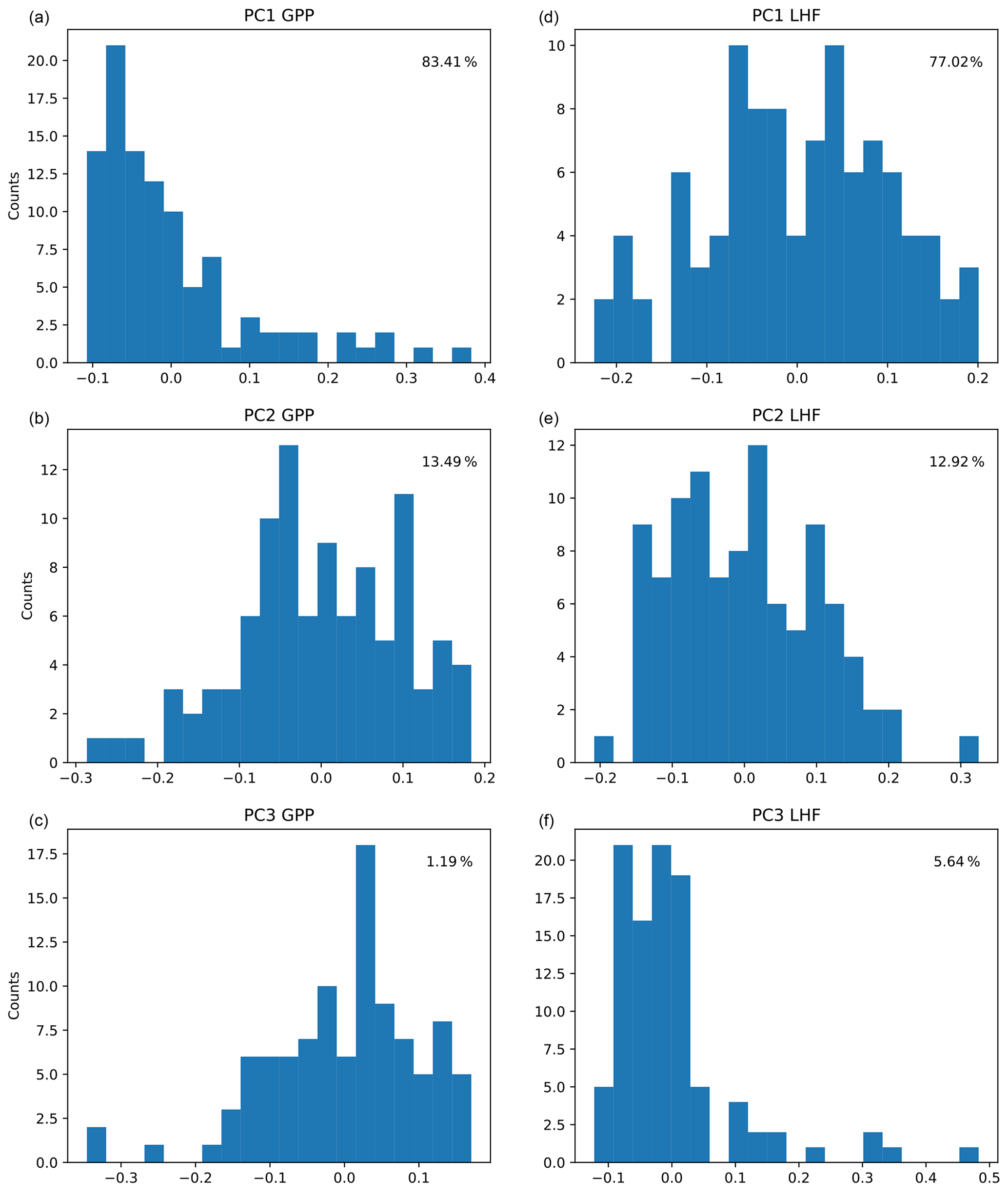
Figure 3 Distributions of the first three principal components (PCs) across CLM PPE ensemble members for GPP (a, b, c) and LHF (d, e, f). The percent variance explained by each mode is shown in each panel in the upper right corner.

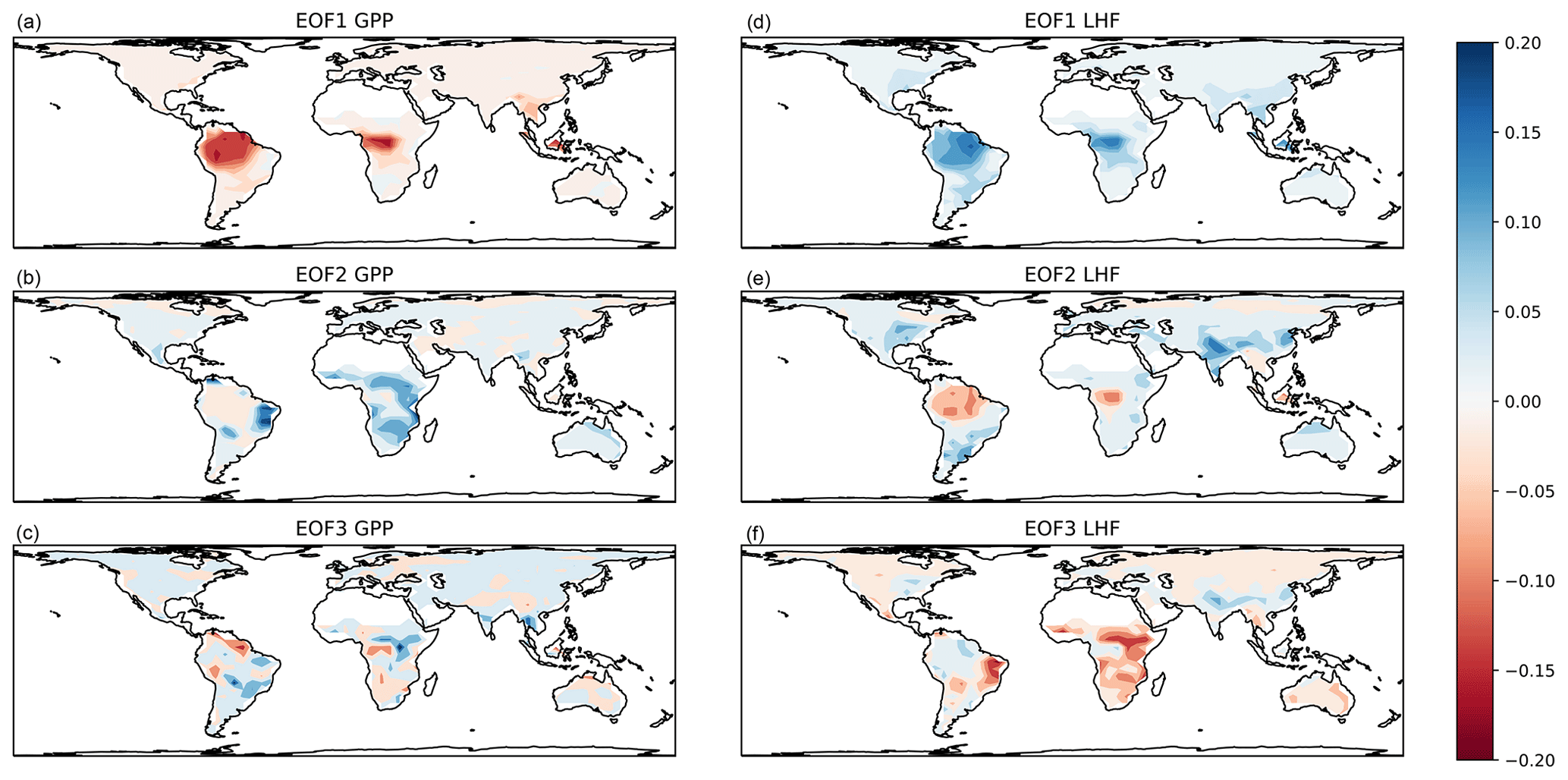
Figure 4 Associated spatial patterns of the first three EOFs for GPP (a, b, c) and LHF (d, e, f).

We utilize 60 % of the ensemble members as training, 20 % for validation during the training process, and keep the remaining 20 % completely separate for out-of-sample testing. We use the mean squared error (MSE) between the network predictions and the actual model output as our skill metric for training the emulator. Our calculation of MSE is detailed in Eq. (4), where n represents the number of ensemble members, U_i represents the actual model output for ensemble member i (calculated in Eq. 3), and ${\widehat{\mathit{U}}}_i$ represents the associated neural network predictions. We calculate the MSE across ensemble members and modes for each subset of the data (training, test, and validation) and compare emulator skill during training with test data and out-of-sample prediction using the validation set. We also consider linear regressions between U and $\widehat{\mathbf{U}}$ for each mode in the validation set and aim to maximize the r² values for all three modes.

$$\begin{array}{}\text{(4)}& \text{MSE}(\mathbf{U},\widehat{\mathbf{U}})={\displaystyle \frac{\mathrm{1}}{n}}\sum _{i=\mathrm{1}}^n({\mathit{U}}_i-\widehat{{\mathit{U}}_i}{)}^{\mathrm{2}}\end{array}$$

During the training process, we iterate on different network configurations to determine the values of some of the important neural network “hyperparameters”, such as number of hidden layers, number of nodes in each layer, activation functions between each layer, optimization algorithm and associated learning rate, batch size, and number of training epochs (Breuel, 2015; Kurth et al., 2018). We find that a network with two hidden layers improves the performance over a single hidden layer (not shown). We also find that a combination of linear and nonlinear activation functions provides the best performance, relative to a single type of activation function. We utilize rectified linear activation for the first hidden layer and hyperbolic tangent for the activation into the second hidden layer (which improved over a logistic sigmoidal function) (Krizhevsky et al., 2017; Breuel, 2015). Finally, we use a linear activation to transition from the second hidden layer into the output layer. We use some regularization in the form of the L2 norm to prevent overfitting and improve generalization (Belkin et al., 2019; Bengio, 2012). We find that the optimization algorithm RMSprop (Tieleman et al., 2012), which utilizes an adaptive learning rate, greatly improves the predictive skill of the network relative to optimization using stochastic gradient descent.

Once the basic structure of each network is defined (two hidden layers with linear and nonlinear activation functions), we test initial learning rates for the RMSprop optimizer and find that a value of 0.005 provides the best tradeoff between computational learning efficiency and accuracy of predictions (Bengio, 2012; Smith, 2017). We also test different batch sizes, defined as the number of samples used to estimate the error gradient at each epoch. Here we also utilize early stopping, where the number of epochs is limited based on the stability of the errors, another method commonly applied to combat overfitting (Belkin et al., 2019; Zhang et al., 2017). A batch size of 30 helps minimize errors during training and improves the ability of the emulator to generalize (Keskar et al., 2017; Bengio, 2012).

With the majority of our hyperparameters set, we then iteratively test the performance of the emulator using between 5 and 15 nodes in each layer and select the best performing configurations based on the mean squared error and predictive skill. For the 5–10 best configurations, we randomly resample the training data 100 times to test the stability of these configurations. This resampling also helps avoid overtraining the network, an important factor considering our small sample size. Our final network configuration is selected based on a combination of high predictive skill and low variability of errors and correlation coefficients. Scatterplots comparing CLM model output with emulator predictions for the first three modes of variance for GPP and LHF are shown in Fig. 5. We further assess emulator performance by analyzing the combined mode predictions to show the error introduced by the EOF approximation and the combined error introduced by the EOF approximation and the emulation. We calculate the root mean squared error (RMSE) across spatial grid points for GPP and LHF relative to FLUXNET-MTE observations of GPP and LHF (Jung et al., 2011). The observations are sampled over the same years as the model simulations (2000–2004), and we calculate the area-weighted anomalies of the observations relative to the PPE ensemble mean. The RMSE is calculated for the original CLM PPE and the reconstructed climatology from the neural network (NN) predictions. We further decompose this error by also calculating the RMSE relative to observations for the reconstructed CLM PPE based on truncating at the first three modes of variability. Figure 6a, b show the error introduced by the EOF approximation, and Fig. 6c, d show the total error from the EOF approximation and the emulation combined. Comparing these top and bottom panels, most of the error comes from the emulation rather than the EOF approximation for both GPP and LHF. However, the emulation performance when viewing the combined mode predictions is still comparable to the performance across individual PC modes as shown in Fig. 5. Figure 6e shows the combined GPP and LHF normalized error performance relative to observations, comparing the NN predictions with the original CLM PPE. The normalized error is calculated in the form of a weighted cost function, which will be discussed further in Sect. 4.2. We also perform a history matching type experiment (Williamson et al., 2015) in this section to study optimal regions of the parameter space, and for reference the error threshold for this experiment is shown as a vertical magenta line in this panel. All panels of Fig. 6 also show the error resulting from the model with default parameter values for comparison.

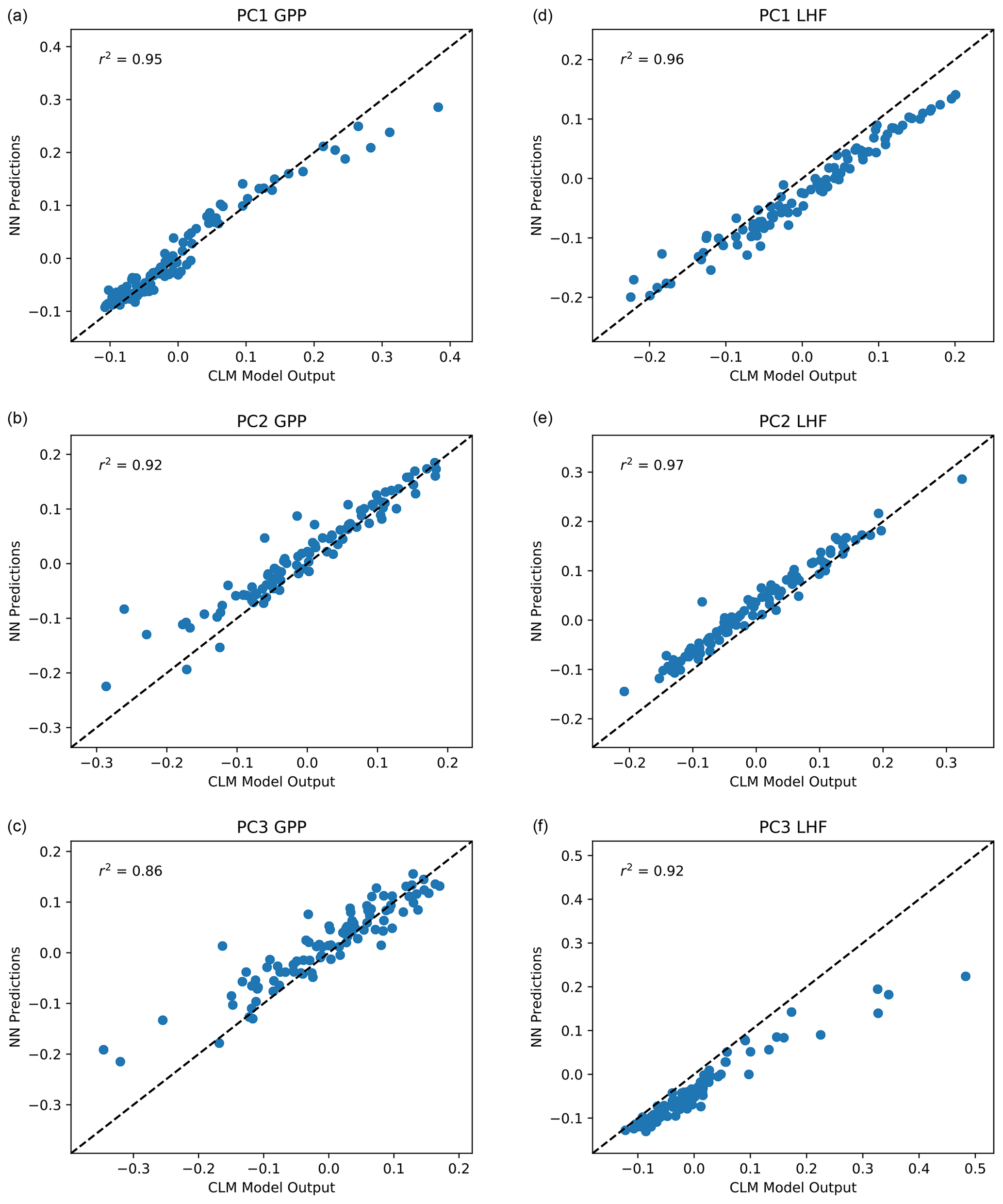
Figure 5 Scatterplot of predicted PC1, PC2, and PC3 for GPP (a, b, c) and LHF (d, e, f) from the neural network emulators versus actual values from CLM output. The one-to-one line is shown in each panel as a dashed black line, and r² values from a linear regression fit are included in each panel in the upper left corner.

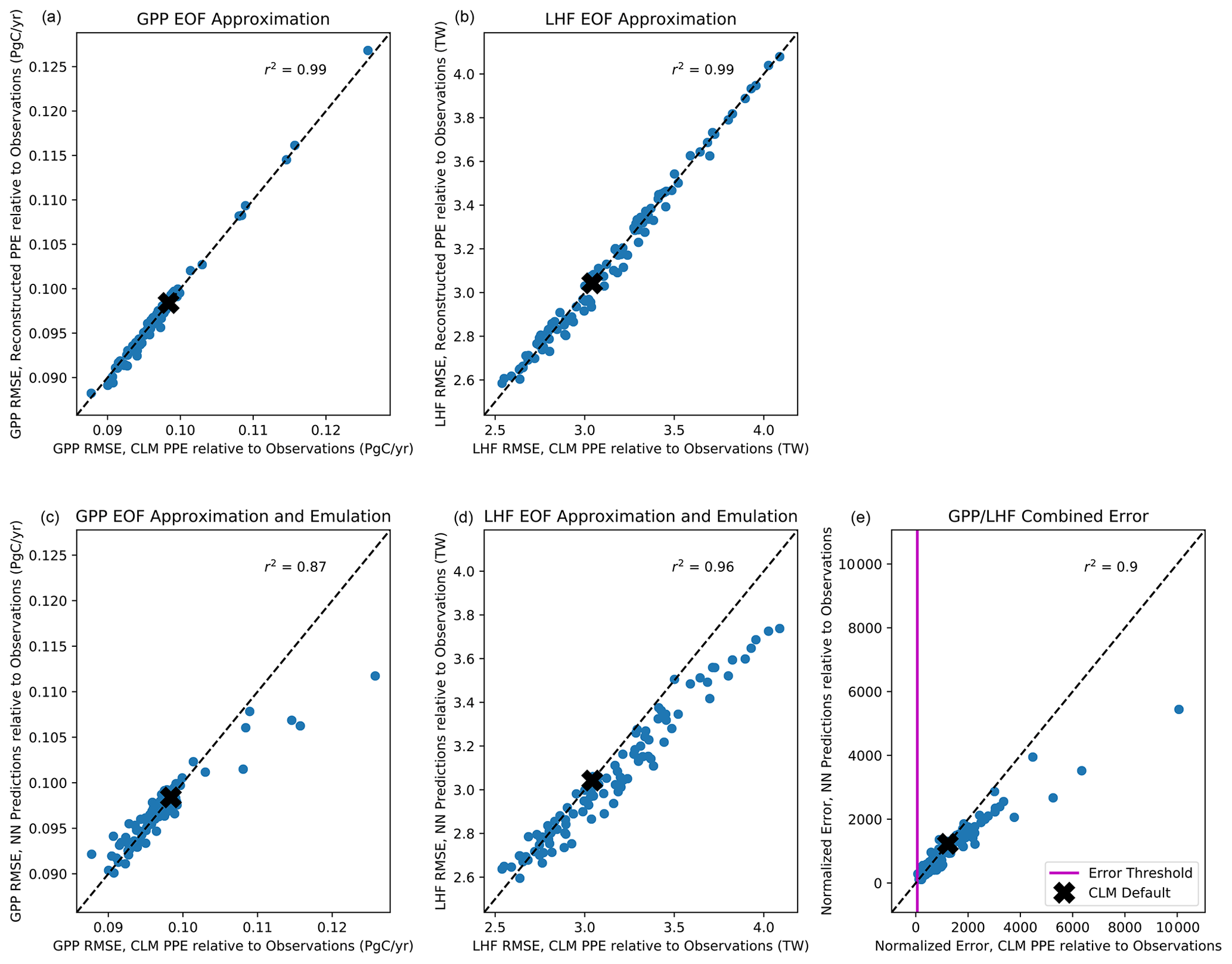
Figure 6 Scatterplot of root mean squared error (RMSE) across spatial grid points for GPP (a, c) and LHF (b, d) from the reconstructed EOF approximation relative to observations (a, b) and the reconstructed neural network (NN) predictions relative to observations (c, d) versus RMSE from CLM PPE relative to observations. Panel (e) shows the combined GPP/LHF normalized error relative to observations for the NN predictions versus the CLM PPE. The error threshold for the history matching experiment described in Sect. 4.2 is shown as a vertical magenta line. The errors resulting from the model with default parameters are shown as a black x in each panel. The one-to-one line is shown in each panel as a dashed black line, and r² values from a linear regression fit are included at the top of each panel.

To provide another check on the performance of the emulator, we produce a second PPE using 100 different random combinations of parameter values for the same set of six parameters, also generated using Latin hypercube sampling but with a different LHC than the first PPE. We then use the emulator trained on the first PPE to test the predictive skill using the information from the second PPE. The predictive skill is comparable, especially for the first two modes, which provides more confidence in the trained emulator and helps support the notion that the network is not overtrained (Fig. S5). Following Fig. 6, we also plot the RMSE comparisons and error breakdown for the second CLM PPE relative to observations (Fig. S6). Again, most of the error comes from the emulation rather than the EOF approximation, and the predictive skill is comparable to the first PPE.

3.2 Interpretation of emulator performance and skill

We use multiple interpretation methods to better understand how the neural network emulator makes its predictions and what it has learned (McGovern et al., 2019). The first method we use is called permutation feature importance, which is an approach to ranking the importance of various model predictors. Permutation feature importance tests the importance of different inputs (in this case, land model parameters) in the predictive skill of the neural network (Gagne et al., 2019; Molnar, 2019). Feature importance is calculated by randomly shuffling the values of one parameter input while preserving others and testing the resulting performance of the emulator. The goal of this method is to determine the impact on emulator skill when the statistical link between a predictor input and the output is severed. The skill metric we use for these tests is the mean squared error between the predictions and the actual values (Eq. 4). A larger value implies that the parameter is more important to the predictive skill of the emulator, because when the link between this particular parameter and the emulator output is broken, the performance degrades and the prediction error increases. We plot the results of the permutation feature importance tests for PC1 of GPP and LHF as bar charts in Fig. 7, with larger bars reflecting greater prediction error and thus implying important information is stored in that parameter. We also plot the original emulator skill (i.e., the mean squared error without any permutations) to better compare the permutation results relative to the control with no permutations. For parameters with error very close to the original emulator skill, this implies that either these parameters are not very important to the predictive skill of the emulator or that the information in these parameters is present in a different predictor (McGovern et al., 2019). We find the permutation results are different for the first modes of GPP and LHF, where the skill of the GPP emulator is dominated by one parameter in particular, kmax, and none of the other parameters is particularly important. However, for LHF, there are several important parameters, including medlynslope, kmax, and dint. These results change when you look at the higher modes of variability, demonstrating that there are different parameters important to predicting different modes of GPP and LHF (Fig. S7).

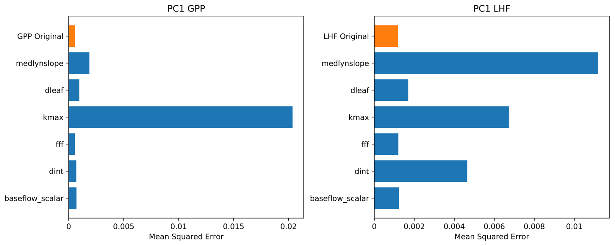
Figure 7 Permutation feature importance test of PC1 for GPP and LHF from the neural network emulators. The top bar (in orange) shows the mean squared error without any permutation (original model skill), and each row (in blue) shows the emulator performance when the information from each parameter is removed, one at a time.

The second method we use is partial dependence plots, a technique to visualize the partial dependence of the predictions on an individual input variable (Friedman, 2001). Partial dependence plots further the analysis of permutation feature importance tests by helping to illuminate why a certain parameter is important (McGovern et al., 2019; Molnar, 2019). These plots show where in the uncertainty range a given parameter is most important to the skill of the emulator. To visualize these results, we first generate a set of 10 fixed values for each parameter by evenly sampling its uncertainty range. Taking one parameter and one fixed value at a time, we then replace all the values for that parameter in the original LHC-generated parameter sets with the fixed value. In this way we are removing any skill from that parameter across the entire ensemble. We then generate predictions using the trained emulator where we have artificially fixed one parameter to the same value across all ensemble members. We repeat for each fixed value and each parameter and calculate separately for GPP and LHF. We then average the predictions across the emulator output to average out the effects of the other predictors. We plot the PC1 results for each parameter in Fig. 8, where each line represents the average prediction across emulator output for the 10 fixed values (shown as points on the bold lines). In this way we can see how the predictions vary across the uncertainty ranges for each parameter. Regions of non-zero slope in the partial dependence plots indicate where in the parameter range the emulator is most sensitive. For example, we see that it is the low end of kmax values that has the greatest impact on the skill of the emulator for PC1 GPP. For PC1 LHF, the parameter medlynslope is important fairly consistently across its range of values. As with feature importance, these results change for the higher modes and highlight the importance of different parameters (Fig. S8 and S9).

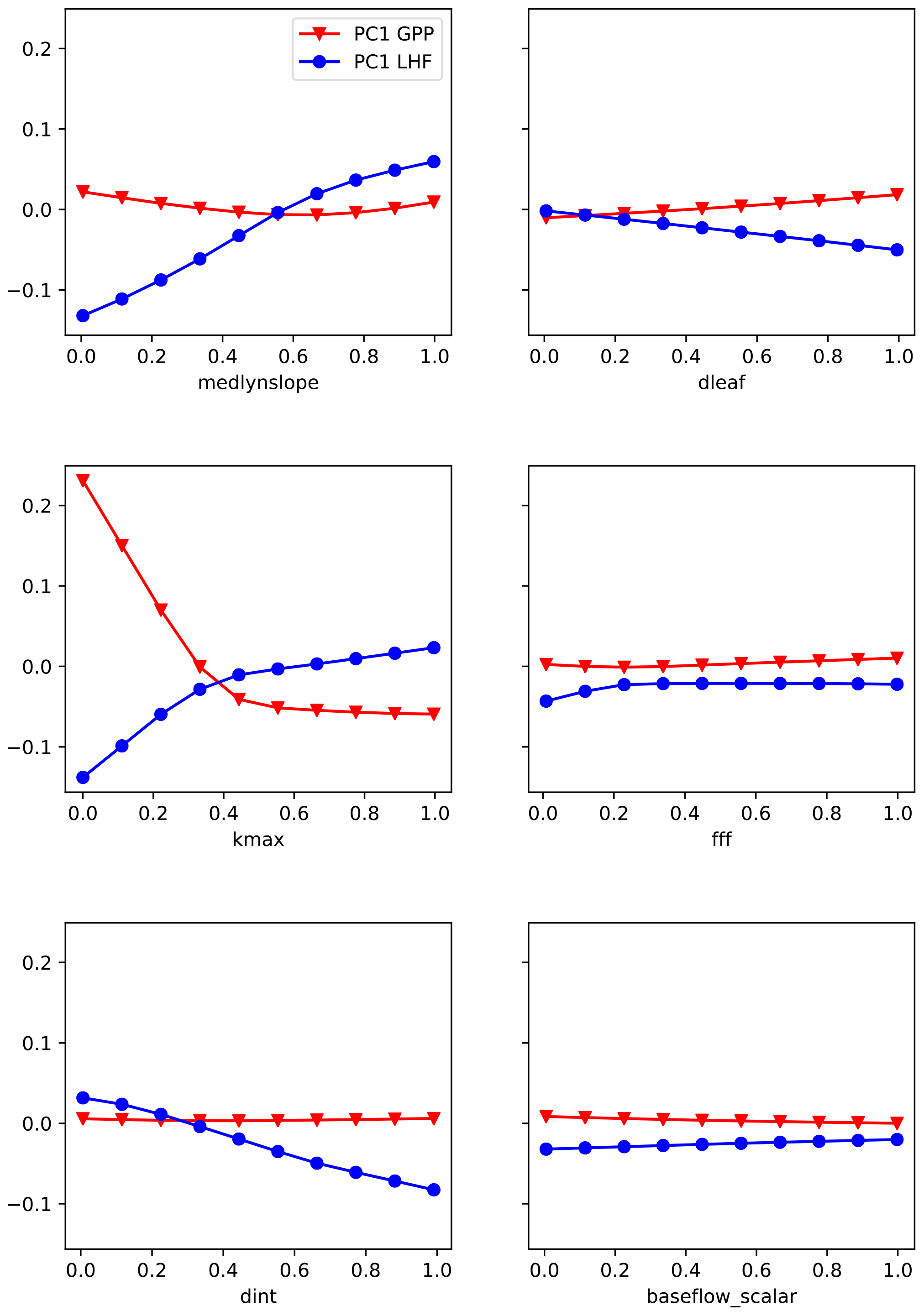
Figure 8 Partial dependence plots of PC1 for GPP (red) and LHF (blue) from the neural network emulators. Circles and triangles denote the fixed values used for predictions with each parameter. The x axis shows the parameter scaling values, and the y axis shows the average prediction of PC1.

3.3 Ensemble inflation

As an additional test of the emulation performance, we utilize the trained neural networks to artificially inflate the PPE ensemble size. Here we are exploiting the full power of emulation, in that we can quickly predict CLM output given new and unseen parameter values. To test the emulation, we generate 1000 random parameter sets using Latin hypercube sampling to more densely span the uncertainty ranges for the six parameters of interest. These parameter sets are fed into the trained emulators to produce predictions for the first three modes of variability for GPP and LHF. The emulation process takes seconds, whereas running CLM globally with this setup to test a given parameter set would take several hours per simulation. The distributions of predictions from the inflated ensemble relative to the original PPE for GPP and LHF are shown in Fig. S10. We see that the predictions with the inflated ensemble replicate both the overall range and the characteristic shape of the original CLM PPE distributions (see also Fig. 3 for the original PPE distributions).

4 Parameter estimation

We next apply our trained emulator of CLM to globally optimize parameter values based on best fit to observations. The neural network emulator can quickly produce predictions of CLM output for a given parameter set, and we aim to optimize the emulation process with the goal of reducing model error. In this section we outline the procedure for producing optimized parameter sets, including details of the observational datasets, construction of the cost function to minimize model error, and optimization results including testing parameter estimates with CLM.

4.1 Observational data

Here we use the FLUXNET-MTE product (Jung et al., 2011) to provide observational targets for our parameter estimation. This dataset includes globally gridded GPP and LHF estimates at 0.5^∘ resolution from 1982 to 2008. We begin by sampling FLUXNET monthly GPP and LHF values from 2000 to 2004 to match the years of the CLM simulations. We regrid the observations to match the CLM output resolution of 4^∘ latitude by 5^∘ longitude using bilinear interpolation. We then calculate area-weighted anomalies for the observations, where the anomalies are calculated relative to the CLM PPE mean. The observed anomalies are then projected into the same EOF space as the PPE to produce observational estimates consistent with the output metrics used to train the neural network. This calculation is detailed in Eq. (5), where X_obs represents the observed anomalies, s and V are taken from the SVD calculation for the PPE (Eq. 3), and U_obs represents the observational targets projected into the same SVD space. We also calculate, as a reference, the default CLM state without any variations in parameter values, where the default values are calculated in a similar manner to the observations. We can then optimize for parameter values that minimize the error with respect to the observational estimates, looking across output variables and modes of variability.

$$\begin{array}{}\text{(5)}& {\mathit{U}}_{\mathrm{obs}}={\mathit{X}}_{\mathrm{obs}}\times (\mathbf{s}\times \mathbf{V}{)}^{-\mathrm{1}}\end{array}$$

4.2 Cost function

With two output variables (GPP and LHF) and three modes of variability for each, we have six targets for parameter calibration. A key question is how to combine them into a single cost function representing model predictive skill relative to observations. Here we calculate the normalized mean squared error of the model predictions relative to observations, with a weighted sum over modes and a separate term for each output variable. The cost function J(p) is detailed in Eq. (6), where ${\widehat{U}}_{v,m}\left(p\right)$ represents the predictions from the neural network emulator for output variable v and mode m as a function of parameter values p. $U_{\mathrm{obs},v,m}$ are the observational targets calculated in Eq. (5), and we normalize by the standard deviation across all observational years (1982–2008, represented by $\mathit{\sigma }\left(U_{{\mathrm{obs}}^{*},v,m}\right)$) in order to account for natural variability using as many years as possible in this dataset. The sum for each variable is weighted by the percent variance explained by each mode (λ_v, m).

$$\begin{array}{}\text{(6)}& J\left(p\right)=\sum _{v=\mathrm{1}}^{\mathrm{2}}\left[\sum _{m=\mathrm{1}}^{\mathrm{3}}{\mathit{\lambda }}_{v,m}{\left({\displaystyle \frac{{\widehat{U}}_{v,m}\left(p\right)-U_{\mathrm{obs},v,m}}{\mathit{\sigma }\left(U_{{\mathrm{obs}}^{*},v,m}\right)}}\right)}^{\mathrm{2}}\right]\end{array}$$

To explore parameter response surfaces of this cost function, we perform a history matching type experiment (Williamson et al., 2015). We generate an additional large Latin hypercube parameter set with 10 million members and predict the PCs for each member using the trained emulators. We then compute the cost function J(p) following Eq. (6) for each member using the emulated PCs. We subset the results, selecting the 1000 members with the smallest normalized error as computed by the cost function. (For reference, the error threshold for this subset of parameter solutions is shown as a vertical magenta line in Fig. 6e.) We then take each parameter pair and plot the distribution of the parameter scaling values. Fig. 9 shows the resulting parameter space, highlighting the regions where the optimal solution would apply. The diagonal panels show the distributions of optimal parameter scaling values for each parameter. For certain parameters (notably dleaf and baseflow_scalar), the range of values is not well constrained by selecting parameter sets with small normalized errors. Other parameters such as fff and dint favor the edges of their uncertainty bounds and also may not be as well constrained by this exercise. However, for the medlynslope and kmax parameters, these plots show where the optimal solutions sit relative to their uncertainty ranges, as well as their relationships with other parameters.

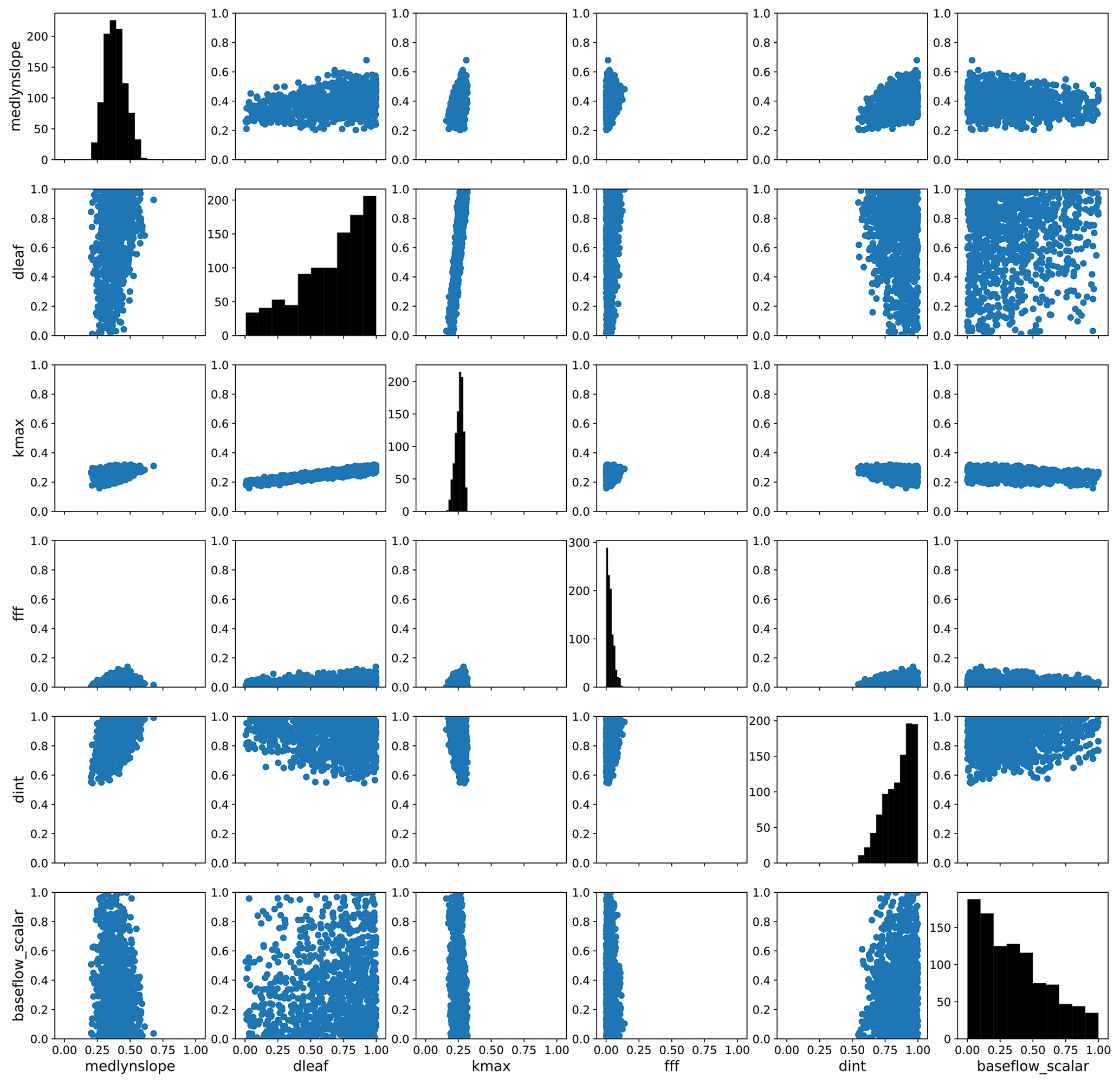
Figure 9 The parameter space of optimal solutions from an additional large emulated ensemble. Here we show a subset of 1000 parameter sets with the smallest predicted normalized error from that ensemble. The axes of these figures show the parameter scaling values, except for the y axes of the diagonals which show the distributions of optimal scaling values for each individual parameter.

4.3 Nonlinear optimization

We use the SciPy optimize function in Python to minimize the cost function J(p) and find optimal parameter values (https://docs.scipy.org/doc/scipy/reference/optimize.html, last access: October 2020). There are many different nonlinear optimization and root finding methods available through this package, and we test several of these algorithms to explore their effectiveness at finding optimal parameter values. In particular, a bounded global nonlinear optimization approach using differential evolution produces the best results by quickly and efficiently searching the solution space (Storn and Price, 1997). We use random initial conditions to initialize the algorithm and impose bounds of [0,1] for each parameter scaling factor, representing the minimum and maximum of the uncertainty ranges.

We also utilize other global methods such as dual annealing (Xiang et al., 1997) and simplicial homology global optimization (SHGO) (Endres et al., 2018) to verify the results. SHGO fails to converge on an optimal solution, while dual annealing produces a similar result to differential evolution but takes several orders of magnitude more iterations and function evaluations. Local optimization methods such as sequential least squares programming (SLSQP), limited-memory bounded Broyden–Fletcher–Goldfarb–Shanno (L-BFGS-B), truncated Newton (TNC), and trust-region constrained tend to get stuck at a local minimum and do not sufficiently explore the parameter space. All of the above methods are referenced in the SciPy package.

To test the sensitivity of our cost function formulation, we repeat the optimization process using an alternate cost function that removes the weighting by modes of variability (λ_v, m in Eq. 6). The resulting parameter values are very similar to the approach using a cost function with mode weighting, demonstrating that this aspect of the cost function is not a significant factor in finding an optimal parameter set in this context.

4.4 CLM test case

Using the optimization results, we translate the parameter scaling factors back to parameter values and run a test simulation with CLM. We use the same model setup as before, spinning up the model for 15 years and using the subsequent 5 years for analysis. The results for the first three modes of GPP and LHF are summarized in Fig. 10. The results for PC1 show that the emulator predictions (blue bars) are very close to the results of the test case (green bars), particularly for PC1 GPP. This feature is less apparent for PC2-3 GPP and PC3 LHF, where the CLM test case is not able to capture the optimized predictions as accurately, possibly due to the noisy nature of the higher modes. Despite this mismatch, these results demonstrate another out-of-sample test of the emulator in predicting CLM output. From the first mode of GPP and LHF we also see that the optimized predictions do indeed match the observations (red bars), suggesting that the emulator has been successfully optimized to match observations for this mode. Furthermore, by using the optimal parameter values in CLM we are able to capture the predictive skill of the emulator and minimize model error. The results for the higher modes vary, but in general the CLM test case with optimal parameters moves the model closer to observations, especially when compared with the default model performance (black bars).

Figure 10 PC1, PC2, and PC3 for GPP (a) and LHF (b) comparing observations, model simulations, and emulator predictions. Observational estimates from FLUXNET are shown as red bars, CLM default values are shown as black bars, the optimized NN predictions are shown as blue bars, and the results of the CLM test case with optimal parameters are shown as green bars.

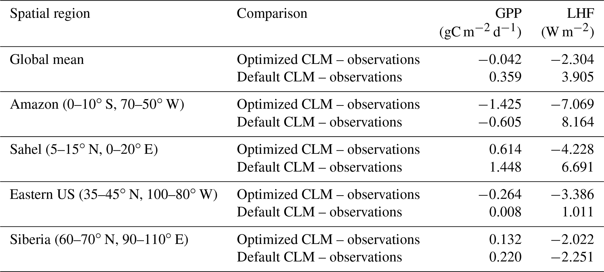
To further investigate the spatial response, we compare the mean bias maps for the optimized CLM test case and the default CLM configuration relative to observations (Fig. 11). We also calculate the global and regional mean biases for GPP and LHF and summarize these in Table 2. We see that the optimized model has some areas of improvement and some areas of degradation when comparing these results with the default model bias. For GPP we are able to decrease the positive biases in the Sahel and other parts of Africa, but in turn the negative bias in the Amazon increases. Positive biases in LHF become negative in the calibrated model, though some areas do show decreases in the bias magnitude. We also calculate the differences for sensible heat flux (FSH), an output variable that we did not calibrate to using the CLM emulator. Encouragingly, we see that areas of negative FSH bias in India and Africa decrease in magnitude with the optimized model, though some areas of positive bias increase. This result demonstrates we are able to achieve some cross-variable benefits to parameter calibration beyond the objectives that were selected for emulation. We also include the mean bias maps for the optimized CLM test case using the alternate cost function formulation that removes weighting by modes of variability (Fig. S11). As stated above, the results are nearly indistinguishable due to the close similarity in the optimal parameter values selected with this alternate cost function.

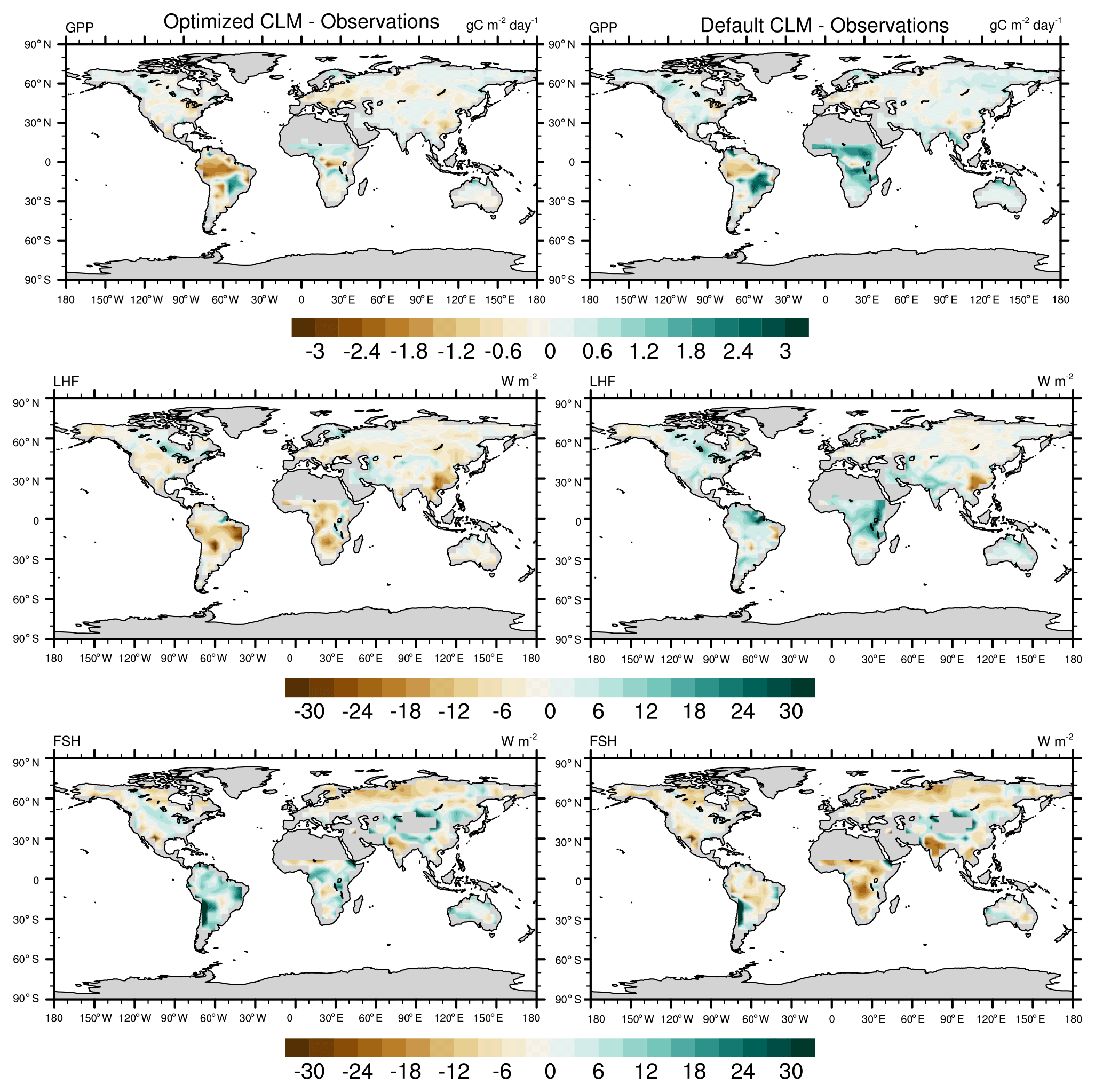
Figure 11 Annual mean bias maps comparing the CLM with optimized parameters (left column) and the CLM default configuration (right column) with observations. The differences are calculated for the calibrated output variables (GPP and LHF), along with sensible heat flux (FSH), an additional model output that we did not calibrate to.

Table 2 Global and regional mean biases for GPP and LHF comparing CLM with optimized parameters and the CLM default configuration with observations.

To highlight the responses in different regions, we also calculate the monthly climatology of GPP and LHF for four different regions representing different biomes (Figs. S12 and S13). The results for the Amazon show that we are unable to capture the phase of the seasonal cycle for GPP with either the default or optimized model, and in fact the seasonal cycle in the optimized model shifts further away from the observations. The seasonality of LHF in the Amazon is better captured, but the overall magnitude in the optimized model is too low. The other regions show some marginal improvement with the optimized model relative to the default model, particularly for the spring and fall in the Sahel and the summer in the eastern US for LHF. LHF in Siberia does not change much at all with the optimized model, though summer GPP does marginally improve there. Winter GPP in the Sahel improves, and while summer GPP gets closer to observations, it is still biased high.

5 Discussion and conclusions

In this study we utilize machine learning to explore parameter uncertainty in a global land model (CLM5). We begin by narrowing the parameter space within our domain of interest, using one-at-a-time sensitivity simulations to identify important biogeophysical parameters in CLM. We utilize multiple methods to assess importance, including global mean sensitivity to multiple model outputs and spatial pattern correlations between parameters across outputs. Our goal is to select overall important parameters that exert control on outputs that cover as much of the planet as possible. By perturbing parameters one at a time we do not include potential parameter interactions, which are a known factor in complex land models (Rosolem et al., 2012). However, by utilizing spatial pattern correlations as a metric for parameter selection, we weight our selection towards parameters without such strong correlations. We also incorporate updated observational data to better constrain uncertainty ranges of sensitive parameters that vary with plant functional type. While it is difficult, in such a process-rich model, to completely avoid relying on expert judgement to identify parameters and their uncertainty ranges, we use this multi-step assessment process in order to be as objective as possible in parameter selection. By identifying important biophysical parameters in CLM5, our approach helps identify which processes are important for accurate land modeling and can help inform observational studies that aim to better quantify these parameters.

With our narrowed set of six parameters, we generate a perturbed parameter ensemble with CLM to span the uncertainty ranges of all parameters and explore parameter interactions. The results of this ensemble show that there are a variety of linear and nonlinear relationships evident between parameters and output fields, highlighting the importance of capturing these diverse relationships. This ensemble is then used to train a set of feed-forward artificial neural networks to act as emulators of CLM. Hyperparameter tuning along with techniques like regularization, early stopping, and resampling of the training data help instill confidence that the neural network is generalizable and not overfitted. While there is still much debate about establishing a procedure for this kind of hyperparameter optimization, we again strive to be as objective and transparent as possible in the construction, training, and validation of the neural network emulators. It is possible our results would change if we had utilized a single neural network emulator to simultaneously predict GPP and LHF, and a single network may be better at preserving correlations between output fields. However, we would be less able to clearly identify which parameters are important to the skill of predicting GPP and LHF individually, as we have shown here.

Our final network configurations provide good predictive skill in emulating the first three modes of annual mean spatial variability for GPP and LHF. We show that the EOF approximation of truncation at the first three modes does not introduce much error, and the minimal error that is present comes from the emulation of those modes by the neural networks. We see comparable performance using a second CLM PPE with the trained neural networks, which gives us additional confidence in the predictive skill of the emulator. While our training dataset is small due to the limited ensemble size, it is encouraging to see that the networks are able to generalize to the second PPE with similar skill. We also explore different interpretation methods such as feature importance and partial dependence plots to better understand the inner workings of the neural networks as emulators for CLM. These methods help illuminate which parameters are most important to the predictive skill of the emulator and why they are important. In particular, we find that the parameter kmax, related to plant hydraulic conductivity (Kennedy et al., 2019), is most important in the predictive skill for the first mode of GPP. Furthermore, kmax shows a strong nonlinear response in predictive skill where the emulator is most sensitive to values at the low end of its uncertainty range. The parameter medlynslope, or the slope of the stomatal conductance–photosynthesis relationship (Medlyn et al., 2011), is important for the first mode of LHF, roughly uniformly across its full uncertainty range. The medlynslope parameter is also important for the second and third modes of GPP, again somewhat consistently across its uncertainty range. The kmax and medlynslope parameters both relate to plant carbon and water use. Due to the strong influence of the tropics on the first modes of GPP and LHF it is perhaps not surprising that these parameters are important for their predictions. The nonlinear response of kmax indicates the parameter range may be too wide and could be narrowed by decreasing the maximum values or by developing PFT-specific values. Plant hydraulic stress models are difficult to constrain due to a sparsity of observations, but work is currently ongoing to address these parameter uncertainties (Kennedy et al., 2019). The parameter dint is shown to be important for the second mode of LHF and the parameter fff for the third mode of LHF. These parameters relate to soil hydrology, and thus they likely influence LHF through soil evaporation and possibly soil water available for transpiration (Swenson and Lawrence, 2014; Niu et al., 2005). The parameter dint is important for PC2 LHF across its full uncertainty range, but fff also shows some nonlinear behavior for PC3 LHF, where the emulator is most sensitive to low values. Again, this could indicate that the ranges of values for fff could be narrowed by decreasing the maximum value, though additional study is needed to better inform the values of these soil hydrology parameters.

We next use the trained emulators to produce globally optimized parameter values for our six parameters based on best fit to observations of GPP and LHF. There are many ways to formulate a cost function to assess model error relative to observational targets (Trudinger et al., 2007). Our approach uses a weighted sum over the first three modes of the squared differences between emulator predictions and observations, normalized by variability in the observations and with separate error terms for GPP and LHF. Our sensitivity test with an alternate cost function shows that the mode weighting is not important to determining the optimization results. We represent observational uncertainty through the normalization term as a substitute for measurement uncertainty or other sources of uncertainty that might arise in the creation of the globally gridded observational products, which are not quantified (Jung et al., 2011; Collier et al., 2018). We do not explicitly include emulator uncertainty in our cost function, or the idea that the emulator is not a perfect representation of CLM (McNeall et al., 2016; Williamson et al., 2015). While we do not expect this uncertainty to be zero, we can begin to quantify it by comparing the emulator predictions for optimized parameters and the results from the model tested with those estimated parameter values. Our test simulation with CLM shows that we can capture the behavior of the optimized predictions for PC1 by using the optimized parameter values in the land model, though the higher modes are not as well captured. This implies there is some uncertainty present in the emulation of PC2 and PC3, perhaps due to the sample size in conjunction with the lower variance associated with these modes. Despite this uncertainty, the CLM test simulation moves the model closer to observations relative to the default for all modes (with the exception of PC3 LHF).

We also explore parameter relationships by visualizing the optimal parameter space for a subset of parameter values where the predicted normalized errors are small. Some parameters are not well constrained by this exercise, and these parameters (dleaf and baseflow_scalar) are also not shown to be important to the predictive skill of the emulators. Other parameters (fff and dint) are shown to sample the edges of their uncertainty bounds, indicating that the range of values chosen for these parameters may not be sufficient to capture optimal solutions. This result echoes what was found utilizing the partial dependence plots for the higher modes of GPP and LHF. Two parameters (medlynslope and kmax) appear to be more constrained by the optimization process and are consistent with parameters found to be important through the permutation feature important tests for different output modes. These parameters will be the focus of further study to better define their range of values and quantify uncertainty. In particular, the relationship between medlynslope and kmax is well constrained by the optimization and relates to the coupling of plant water stress and stomatal conductance. The new plant hydraulic stress formulation in CLM5 implements this coupling through a water stress factor to better incorporate theory of plant hydraulics (Kennedy et al., 2019). Future process-based modeling could further this approach by directly modeling hydraulic limitation as part of stomatal conductance (Anderegg et al., 2018).

For the optimized model relative to the default configuration, we find that mean spatial biases persist and in some cases worsen. For example, we cannot simultaneously correct mean GPP biases in the Amazon and Congo, similar to results shown in McNeall et al. (2016). This is suggestive of additional sources of uncertainty and structural biases present in the default model configuration (e.g., forcing uncertainty, epistemic uncertainty, or additional parametric uncertainty), which cannot be tuned with the limited set of parameters we have selected for this analysis. It has also been shown previously that it is difficult to find global optimal parameter values which consistently improve skill in a climate model (Jackson et al., 2008; Williamson et al., 2015; Li et al., 2018), and we find a similar outcome when studying biophysical processes with a land model. Cai et al. (2019) calibrated evapotranspiration (ET) across multiple paired FLUXNET sites in the Energy Exascale Earth System Model Land Model and found a reduction in the mean annual bias of ET when the global model was tested with the optimized parameters. This study demonstrates the potential for site-level calibration to improve a global model simulation. They also highlighted the importance of stomatal conductance and soil moisture related parameters, similar to the parameters we found to be most sensitive in CLM5. Li et al. (2018) found a reduction in GPP and LHF error using optimized parameter values in the CABLE and JULES land models; however, this reduction was not consistent across PFTs nor was it consistent across all land area. Furthermore, the differences between the land models increased when both were calibrated to the same observations. Both studies reiterate the difficulty of globally calibrating a limited set of land model parameters and discuss additional sources of uncertainty contributing to model biases and inter-model differences.

Parameter estimation results will always be sensitive to the choice of cost function and how additional sources of uncertainty are accounted for (Fer et al., 2018; Jackson et al., 2008; Li et al., 2019; Ray et al., 2015). Though we account for multiple CLM outputs in the form of GPP and LHF, we combine them into a single objective cost function whereas a multi-objective approach could help avoid introducing additional biases into the calibration process (Rosolem et al., 2013). In the future we plan to explore different versions of cost functions to account for sources of uncertainty that we do not sample with this study, including structural uncertainty. Structural uncertainty relates to uncertainty in process representation, including how model equations are formulated. While parametric uncertainty can be explored through scrutinizing choices of parameter values, quantifying structural uncertainty is less clearly defined. The United Kingdom probabilistic climate projections (Murphy et al., 2009, 2007) define structural uncertainty using a multi-model ensemble (MME). The reasoning is that the MME represents a variety of structural choices and can represent this source of uncertainty outside of what a single model can achieve, assuming the MME is made up of “state-of-the-art” climate models that have been validated against historical observations (Sexton et al., 2012; Sexton and Murphy, 2012). However, this approach relies on the assumption that the MME is composed of climate models which are all unique representations of the true climate, while there is evidence that state-of-the-art climate models such as those participating in the Coupled Model Intercomparison Project (CMIP) share components and model development processes, which implies that they may also have common limitations (Sanderson and Knutti, 2012; Eyring et al., 2019).

There are a variety of limitations to our model setup. For the purposes of fully exploring the dynamics of the biogeophysics domain of CLM, we use offline CLM simulations without active biogeochemistry, land use change, or vegetation dynamics and thus are limited to a specific set of processes. We also do not account for cross-PFT interactions within parameters which vary across PFTs. While our approach using consistent scaling factors still allows for different uncertainty ranges for PFTs, our calibration results do not reflect possible variations in the sampling of PFT-specific values for a given parameter. This is primarily due to computational challenges in properly sampling PFT-varying parameters as demonstrated in prior work, though future study will consider possible approaches to better account for interactions between different PFTs. Our offline CLM simulations use a specific 5-year period of atmospheric forcing data, and our results could be dependent on the choice of time period. This choice is somewhat constrained by available observational years, though we could also test additional 5-year or longer periods where we have observations to calibrate the model. The choice of atmospheric forcing data is based on best performance with CLM5 (Lawrence et al., 2019). While our model resolution is low and the simulation length is relatively short, these tradeoffs allow us to perform a global sensitivity analysis and parameter estimation with greater computational efficiency.

Our methodology also uses a smaller subset of output variables (GPP and LHF) for parameter calibration than the larger set of seven biophysical output variables used during the parameter selection stage. For the calibration we are somewhat limited by the availability of globally gridded observational products. However, we expect the results to depend on exactly which output variables are used in the calibration (Keenan et al., 2011). We are able to capture some additional benefits to calibration by reducing regional biases in sensible heat flux, despite not explicitly tuning to this output variable. It is an open question as to how many and which calibration fields should be utilized in a model tuning exercise, along with what metrics should be used to assess model biases and changes in model skill (Mendoza et al., 2015; Fer et al., 2018). Here we use annual mean spatial variability as determined by EOF analysis and thus do not consider seasonal cycle changes or interannual variability. As our monthly climatology results show, we gain some marginal improvement in certain regions and seasons, but we would not expect to see significant improvements due to not calibrating specifically to the seasonal cycle in these locations. In the future we plan to explore additional observational datasets and assessment metrics using the International Land Model Benchmarking (ILAMB) system (Collier et al., 2018).

As model sophistication and process representation increase, it is important to acknowledge there is a tradeoff between model complexity and model error (Saltelli, 2019). Our study provides an example of a mechanistic framework for evaluating parameter uncertainty in a complex global land model. By utilizing machine learning to build a fast emulator of the land model, we can more efficiently optimize parameter values with respect to observations and understand the different sources of uncertainty contributing to predictions in terrestrial processes.