the Creative Commons Attribution 4.0 License.
the Creative Commons Attribution 4.0 License.
 | 07 Apr 2022
Deep learning for statistical downscaling of sea states
Marceau Michel
Said Obakrim
Nicolas Raillard
Pierre Ailliot
Valérie Monbet
Numerous marine applications require the prediction of medium- and long-term sea states. Climate models are mainly focused on the description of the atmosphere and global ocean variables, most often on a synoptic scale. Downscaling models exist to move from these atmospheric variables to the integral descriptors of the surface state; however, they are most often complex numerical models based on physics equations that entail significant computational costs. Statistical downscaling models provide an alternative to these models by constructing an empirical relationship between large-scale atmospheric variables and local variables, using historical data. Among the existing methods, deep learning methods are attracting increasing interest because of their ability to build hierarchical representations of features. To our knowledge, these models have not yet been tested in the case of sea state downscaling. In this study, a convolutional neural network (CNN)-type model for the prediction of significant wave height from wind fields in the Bay of Biscay is presented. The performance of this model is evaluated at several points and compared to other statistical downscaling methods and to WAVEWATCH III hindcast databases. The results obtained from these different stations show that the proposed method is suitable for predicting sea states. The observed performances are superior to those of the other statistical downscaling methods studied but remain inferior to those of the physical models. The low computational cost and the ease of implementation are, however, important assets for this method.
- Article
(2531 KB) - Full-text XML
- BibTeX
- EndNote


The prediction of sea states meets multiple maritime needs. In particular, waves are the major environmental forcing at sea. Their prediction is, therefore, required for the sizing of marine structures, for the implementation of marine energy converters, or for seakeeping. Because of the long life of these structures, engineers need medium- and long-term future projections, as well as extensive time series. Indeed, the design of offshore structures usually requires a 100-year return period (Ewans and Jonathan, 2012). Other applications, such as coastal flood risk prevention, demand the characterization of wave climatology (Idier et al., 2020). For atmospheric variables, these predictions are provided by general circulation models (GCMs), but these models are coarse and hardly predict oceanic variables. To move from GCMs to the oceanographic predictions needed by industry and policy makers, dynamical and statistical downscaling (SD) methods have been developed.
In perfect prognosis statistical downscaling, an empirical relationship is built between large-scale atmospheric predictors and local wave parameters. Its main advantage is its low computational cost compared to numerical models. The efficiency of these methods allows us to explore different GCM scenarios and models, as well as to carry out several runs to estimate the uncertainties (Trzaska and Schnarr, 2014). This type of model has already been implemented in several studies for the prediction of ocean waves (Laugel et al., 2014; Wang et al., 2010). Among the possible approaches for statistical downscaling problems, machine learning approaches and, more precisely, deep learning ones have shown their interest, thanks to their ability to extract high-level feature representations in a hierarchical way (Baño-Medina et al., 2020). However, these approaches are still perceived as black boxes, which explains the lack of confidence in these models among the climate community, especially for climate change issues. Nevertheless, there are increasing calls to encourage research towards the understanding of deep neural networks in climate science (Reichstein et al., 2019).
In this study, a deep neural network is developed to describe the relationship between global wind and local sea state, considering the spatial structure of this relationship that is introduced. The choice was made to focus on the prediction of the significant wave height (Hs), which is probably the more important sea state parameter for many applications. After the presentation of the developed architecture, the results of the network are evaluated on a point located in the Bay of Biscay. Then, its performances are compared to two classical statistical downscaling methods. Finally, the prediction made by the neural network trained using buoy data and the prediction from a numerical model are compared. The Bay of Biscay has been chosen because of the availability of the hindcast database. This region is characterized by a significant proportion of multimodal sea states with swells generated all across North Atlantic Ocean and wind sea waves that can be significant. It was developed in order to characterize precisely the near-shore sea state conditions for the production and design of marine renewable energy (MRE) devices, such as wave energy converters (WECs; Payne et al., 2021). The proposed methodology could be extended for any other locations, as soon as sufficient data are available.
The following three paragraphs describe the main characteristics of the datasets used in this study.
2.1 Climate Forecast System Reanalysis
The Climate Forecast System Reanalysis (CFSR) is a hindcast database (Saha et al., 2010). Wind and other environmental variables (humidity, pressure, etc.) are recomputed with a homogeneous model and data assimilation system to eliminate fictitious trends caused by model and data assimilation changes in real time. The main purpose of this type of treatment is to obtain consistent datasets for the study of climate.
Only 10 m wind components U10 and V10 are extracted with a degraded space–time resolution of 3 h for the time resolution and half a degree in latitude and longitude for the spatial resolution. The predictors of the proposed method are derived from these components. Their construction is detailed in Sect. 3.1.
2.2 WAVEWATCH III numerical models
Predicting wave climatology is particularly complex due to the random nature of the ocean, the lack of data, and the difference in scale between the phenomena. Numerical wave prediction models are powerful tools to address this problem, based on the physics of the phenomenon (Thomas and Dwarakish, 2015). WAVEWATCH III is a spectral-phase average wave model based on a discretization of the energy balance equation with finite differences in time, as follows:
where k is the wavenumber and E(k) the energy spectrum. The left-hand side constitutes a local term and an advective term moving at the group velocity, cg. The energy supplied by the wind accounted for in the source term Sin is redistributed via the non-linear wave interaction term Snl. The dissipation term Sds addresses the energy loss due to wave breaking caused by high wave steepness (Ardhuin, 2021). As it is a phase average model, WAVEWATCH III cannot simulate diffraction phenomena.
WAVEWATCH III's model accuracy depends on the one of the forcing fields and parameterization of the source terms and on the effect of the numerical schemes (Roland and Ardhuin, 2014). In deep water, the predominant forcing is the wind, followed by currents and water height. This order is reversed in coastal areas.
Hs and other wave parameters, such as Tp and wave direction, are directly estimated from the energy spectrum E(k). For reasons of memory limitation, the spectra are only stored for a few nodes. For the remaining nodes, only the wave parameters are available in the model output.
In this study, data from two hindcast databases using the WAVEWATCH III model are exploited as follows:
-
HOMERE. This specific hindcast database has been developed by Ifremer (French National Institute for Ocean Science) for the “assessment of sea-state climatologies to support research and engineering activities related to the development of marine renewable energies over the Bay of Biscay and the Channel” (Boudière et al., 2013). This model takes realistic sea bed roughness mapping into account. The forcing considered includes CFSR wind, water levels, and tidal currents computed using the MARS 2D hydrodynamic model (Lazure and Dumas, 2007). The HOMERE mesh consists of an unstructured grid built from the depth and wave propagation velocity. The nodes are spaced up to 10 km offshore and only 200 m near the coast.
-
RESOURCECODE (or RSCODE). This hindcast database is the result of a consortium of academic expertise, industry leaders, and research centers to which Ifremer belongs. The development and expansion of the HOMERE MetOcean hindcast database is a central point of this project. Unlike the latter, the wind forcing is derived from the ERA5 database.
Among the parameters describing the sea state, it was decided to focus only on the Hs, which, therefore, constitutes the predictand.
2.3 In situ measurements
In situ data are difficult to use in statistical downscaling models. Indeed, deep learning models usually require a large amount of data to be fitted. In situ data often suffer from too short a recording (less than a decade and missing values). Sea state data from satellite altimetry are particularly complex to use because of their sparsity. Buoys provide high-frequency wave measurements at their location. However, buoys with a sufficiently long and continuous history are rather rare, and their spatial repartition is sparse.
The idea of a ground truth can be misleading, and there are challenges in using existing in situ wave measurements. Indeed, data from physical measurements are noisy, which may induce bias and extra variances in the models. Moreover, a buoy estimates the significant wave height from its own motion. Thus, the characteristics of the buoy, such as its size, composition, or structure, as well as the characteristics of the sensor and the processing chain, can alter the estimation of Hs (Ardhuin et al., 2019). Several studies have quantified these measurement errors. For example, some buoys overestimate wave heights by 56 % in hurricane conditions, while measurements from light vessels have a systematic bias, causing an underestimation of high waves (Anderson et al., 2016). In this study, in situ data from buoys have been chosen because they remain the most suitable for the learning method we have developed.
The statistical downscaling method presented in this study is a deep learning model. Deep learning algorithms have gained a large popularity recently because they outperform other prediction algorithms in many fields. The rapid expansion of deep learning has been allowed by the increase of processing power, the amount of available data, and the development of more advanced optimization algorithms. Deep learning models usually involve a huge number of parameters; however, they have good generalization capacities, and methods exist to help interpret the different levels of the network (Gagne et al., 2019). To obtain better performances and to facilitate learning by reducing the dimensionality of the predictor, this model does not work directly on 10 m wind but on a projected and time-shifted wind. The following paragraph describes the construction of the predictors used as input to the proposed model.
3.1 Predictors
The predictors introduced here have been proposed in Obakrim et al. (2022) for a linear statistical downscaling model for the significant wave height. They are based on some simplified physics rules. In particular, the deep-water hypothesis (depth ≥ wavelength) is assumed to be true. At this depth, the energy of the wave is reduced by a factor of exp (π)≈25 compared to the surface (Ardhuin, 2021). Under this hypothesis, the wind can be considered as the only forcing source.
At a given time, the wave field is the combination of the swells generated over long distances, often several days before, and wind sea waves generated by the local wind. It is, therefore, important that the predictors consider the complex phenomenon of wave generation and the non-instantaneous and non-local relationship between wind and waves. Therefore, two sets of predictors are needed, i.e., a local and global predictor, denoted, respectively, as Xl and Xg in the sequel. This approach has already been tested by taking the pressure field as the forcing (Camus et al., 2014). Unlike pressure, wind is represented by two components, i.e., zonal and meridional. Assuming that waves travel along a great circle path (Pérez et al., 2014), wind can be reduced to a single component by projection into the bearing of the target point. Many CFSR wind sources are then masked by continents or islands. Fig. 1 shows the remaining wind sources for the station selected in the Bay of Biscay (see Sect. 4).
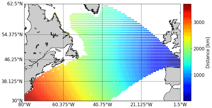
Figure 1Distance to the point of interest.
The global predictor component, , is defined as the mean of the squared projected wind, , on the time window at location j.
The estimated temporal width controls the length of the time window, and estimates the wave travel time. These last two parameters are estimated for each point by maximizing the correlation between the Hs at the target location and the predictor : . The parameters fields obtained by this method are shown in Fig. 2.
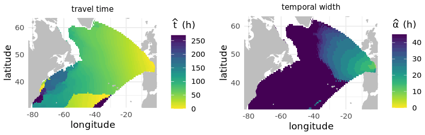
Figure 2Estimated travel time (left). Estimated temporal width in hours (right; from Obakrim et al., 2022).
The local predictor Xl is defined as follows:
in which U is the speed of the local 10 m wind, and F is the fetch. The fetch is the length of the region over which the waves have been generated. The fetch can be difficult to define precisely in open sea (Ardhuin, 2021). In this study, it is defined as the minimum between the distance to the nearest coast in the wind incidence azimuth and 500 km.
3.2 Convolutional neuronal network
Deep learning techniques are promising approaches for statistical downscaling because of their ability to learn spatial features from huge spatiotemporal datasets. The model presented in this paper is a convolutional neural network (CNN). It is inspired by the CNN-PR (pattern recognition) network, using standard topologies from pattern recognition for precipitation downscaling presented in Baño-Medina et al. (2020).
The use of CNN for the statistical downscaling of the sea state has been motivated by properties of CNN that are interesting for the prediction of wind generated waves, as follows:
-
Shared-weight architecture of kernels. For each filter of the convolution layer, it is the same kernel that runs through the input matrix. Thus, when a meteorological event of the same magnitude appears at one position or another on the projected and time-shifted wind map, the result of the convolution operation on the output layer will be the same. CNN are equivariant in translations (Mouton et al., 2020).
-
Pooling. The pooling operation corresponds to the block maximizing of the output layer. When two similar phenomena appear at two close positions, they generate the same output after this operation. CNN are invariant to small translations.
-
Rectified linear activation function (ReLU). The ReLU is the piecewise linear function that is zero for negative values and equal to the identity for positive values. This operation is applied to all neurons of an output layer. It allows one to select the information to be sent to the next layer, thus helping it to learn complex patterns. This operation favors the consideration of non-linear interactions.
To consider the spatiotemporal relationship between wind and waves, more complex architectures, such as 3D-CNN or long short-term memory (LSTM) have been experimented with for 3D-projected wind maps, with the third dimension being time, but they did not offer better performances. For this approach, the wind maps projected over the period were concatenated to form the global predictor. The main problem encountered was the memory management, which imposed a reduction in the spatial and temporal resolution of the data.
3.3 Architecture
Sea state is the result of the combination of wind sea wave and swell. Thus, the model needs to take both wave systems into consideration. This is realized by implementing a hybrid CNN model, HCNN, which takes two inputs, i.e., the global and local predictor. Figure 3 shows a schematic view of the network architecture.
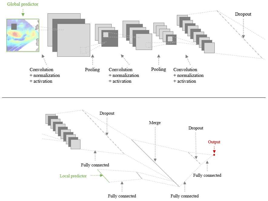
This neural network has been implemented with the Python deep learning library Keras (https://github.com/keras-team/keras, last access: 5 October 2021). The different layers used in the model are as follows:
-
ZeroPadding2D. This adds rows and columns of zeros at the top, bottom, left, and right side of the input to conserve its spatial dimensions (height and width) during the convolution operation.
-
Conv2D. This applies the convolution operation.
-
BatchNormalization. This normalizes the output to make the network more stable during training.
-
MaxPooling2D. This downsamples the input along its spatial dimensions by taking the maximum value over an input window.
-
Concatenate. This concatenates the two inputs.
-
Flatten. This flattens the input (which is mandatory before applying a dense layer).
-
Dense. This applies a regular, densely connected neural network layer.
-
Dropout. This randomly sets input units to zero, which helps prevent overfitting.
The three successive convolution layers, respectively, have 10, 25, and 50 filters. The penultimate layer contains 50 neurons.
The local predictor is normalized before being fed into the neural network to improve numerical stability of the model and its computational efficiency (Shanker et al., 1996). The Adam optimizer is a stochastic gradient descent algorithm in which individual adaptive learning rates are computed for different parameters from the estimates of the first and second moments of the gradients. It was chosen because its hyperparameters have an intuitive interpretation and typically require little tuning (Kingma and Ba, 2015). In addition, the Adam optimization algorithm can handle sparse gradients on noisy problems. The selected loss function is the mean squared error (MSE).
This neural network was trained using data from a point in the Bay of Biscay (located at coordinates 45.25∘ N, 1.61∘ W), belonging to the mesh of the HOMERE database (node no. 7818). This point is located on the continental shelf at a depth of about 55 m. In Sects. 4 and 5, the Hs of HOMERE is chosen as the reference value and is referred to as the target Hs. The time series of Hs is presented on the top panel of Fig. 4. The mean value of the target Hs is 1.92 m (min 0.25 m; max 10.56 m).

Figure 4A 3 h time series (a) and the histogram of Hs (b) at node no. 7818. Results were obtained using the HOMERE dataset.
4.1 Metrics
To evaluate the performance of downscaling methods, classical metrics are used. T and P denote, respectively, the value of the target Hs and the predicted one. The cardinal of the time series is n.
The root mean squared error (RMSE) is the measure of the accuracy, as follows:
The Pearson's correlation coefficient is the linear correlation between two datasets, as follows:
The scatter index is the prediction error normalized by mean of observations and debiased, good metric to quantify the dispersion of the scatterplot and to compare performances at different stations, as follows:
The RMSE of errors greater than the 95th quantile of the error is as follows:
In addition to these statistical indicators, the scatterplot and the quantile–quantile plot are presented. The scatterplot allows one to observe the deviation of the prediction from the identity function. The quantile–quantile plot allows one to observe the adequacy of the distribution of the predicted values with the reference dataset.
4.2 Cross-validation
The performance of the HCNN model is evaluated through seven-fold cross-validation. To do so, the dataset is divided into seven periods of 3 consecutive years. Each of these periods is then successively taken as a validation dataset, with the rest of the data being used for learning. For each of these iterations, five models are trained, and the grand mean of each score is computed on each fold. The training of five individual models is a robust approach to evaluating the skills of deep learning models that are stochastic because of their use of randomness during training, particularly because of the initialization to a random state and the use of stochastic gradient descent algorithms.
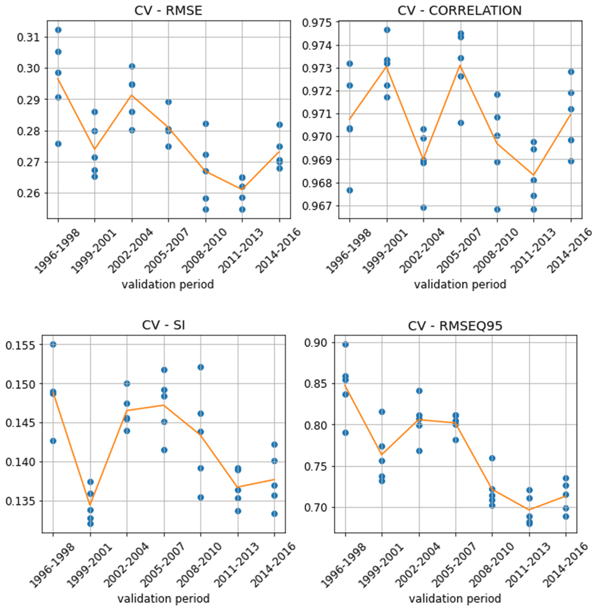
Figure 5Statistical scores for each fold (the orange curve is the average score for each fold).
According to Fig. 5, HCNN gives results of the same order of magnitude over each validation period. The variations observed are justified by the differences in climatology specific to each period. The standard deviation of the HOMERE Hs over the validation period (see Fig. 6) is indeed correlated with the RMSE (ρ: 0.65).

Since the performances of the HCNN model are homogeneous on each of the folds, only the last one is kept to conduct an in-depth study of the performances of the model. The selected training and validation datasets are as follows:
-
Train – 13 January 1994 to 31 December 2013 (size of 58 341)
-
Validation – 1 January 2014 to 31 December 2016 (size of 8767).
4.3 Results of the validation
The results over the test period are satisfactory. The RMSE is 27 cm, which is 14 % of the mean value of the target Hs.
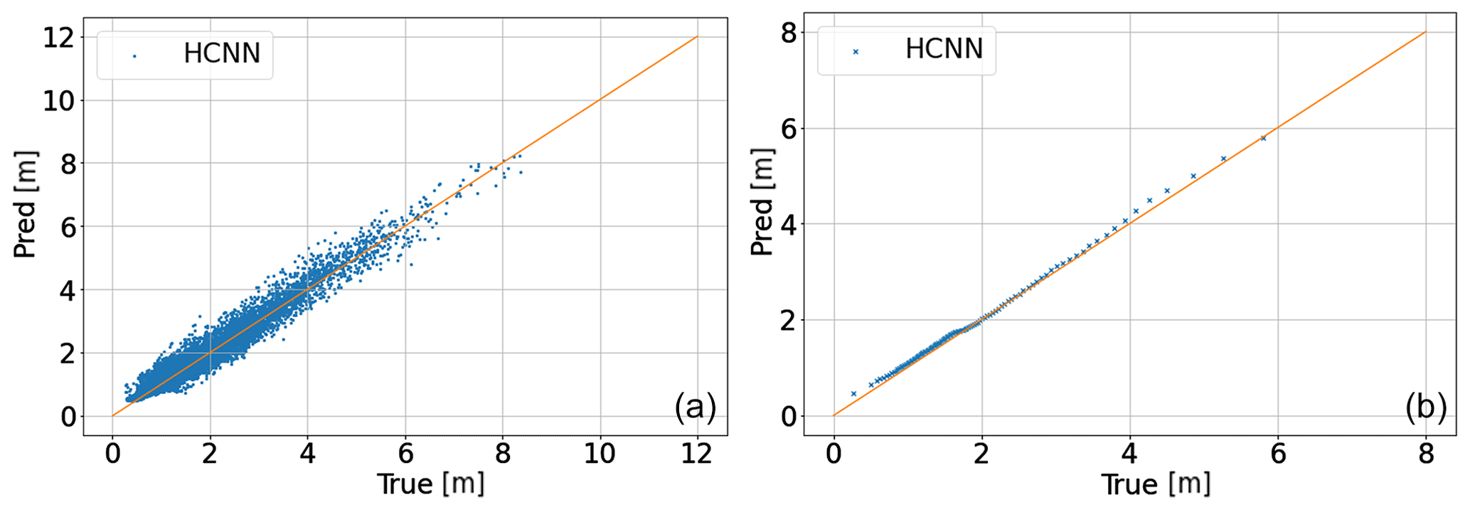
The plots are consistent with the indicators previously outlined. The scatterplot shows a rather weak dispersion around the diagonal line. Moreover, there is no outlier (point very far from this line). The quantile–quantile diagram shows that the distribution of Hs is well reproduced.
4.4 Physical interpretation of the residuals
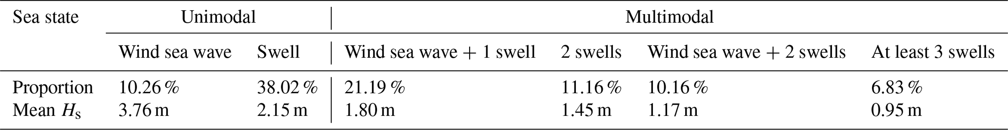
The significant wave height derived from the energy spectrum gives an overall description of the sea state. However, it has been highlighted that a sea state is generally made of wind waves caused by local winds and several swell trains propagated over large distances. To better understand the performance of the method, it is interesting to know how much of these different components are predicted. Energy spectrum partitioning methods have been developed to identify these components. In the output of HOMERE, the partitioning is obtained using the WaveSEP (Wave Spectrum Energy Partitioning) method, which is based on a watershed algorithm (Tracy et al., 2007).
The developed neural network is unable to determine this partitioning. Yet, it is possible to use the classification of wave systems described in Maisondieu (2017) to analyze the performance of the HCNN model. The following six possible combinations of sea states are identified in increasing order of complexity: wind sea wave, swell, wind sea wave + 1 swell, 2 swells, wind sea wave + 2 swells, and at least 3 swells. The following table describes the proportion of each sea state during the test period defined above.
Table 1Proportion and mean of target Hs of each sea state during the test period selected for node no. 7818.
The following bar plot shows the value of the four statistical indicators previously introduced, plus the bias, for each of the six possible combination of sea states.
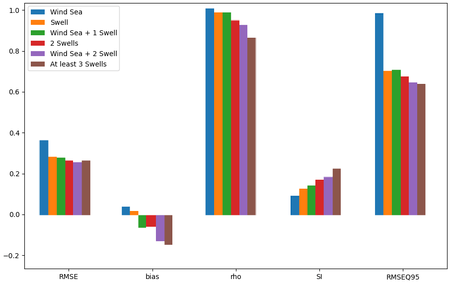
Figure 8Bar plot of prediction scores for each sea state during the test period selected for node no. 7818.
According to Fig. 8, RMSE and RMSEQ95 are higher for wind sea waves and are almost identical for the other sea states. However, the correlation decreases and the scatter index, which gives similar information, increases with the complexity of the sea states. There are two hypotheses that can explain this result. On the one hand, the chosen cost function (MSE) penalizes the errors indifferently for low and high Hs. However, as the complexity of the sea state increases, the average Hs decreases, as shown in Table 2. Since the value of SI is normalized by this average value, it is therefore normal that it increases. On the other hand, this evolution of the error may also be explained by the non-linear interactions between the different wave systems; the more complex the sea state, the more difficult the prediction will be. It is also interesting to observe the bias value which shows an overestimation of complex sea states and an underestimation of unimodal sea states characterized by higher Hs. Finally, RMSEQ95 shows that the most significant errors are associated with wind sea waves. This is probably due to the important simplification made on the calculation of the fetch, which is an important parameter for the generation of wind sea waves.
4.5 Impact of spatial and temporal windows
The previous results were obtained using all available history and all points that are not masked by an island or continent. However, it is reasonable to assume that, beyond a certain distance, the waves generated by the wind do not reach the target location (or only a small fraction of their energy) and that the model does not need such an amount of data. To determine the width of the spatial and temporal window, several models are trained by gradually widening them. The two RMSE indicators are used to quantify the evolution of the prediction error. Due to the geometry of the global predictor (see Fig. 1), the search for the spatial window is simplified to the search for the optimal range of longitudes, which is hereafter referred to as Δ longitude. Since France is a natural barrier east of the Bay of Biscay, only the western longitude limit has been adjusted.
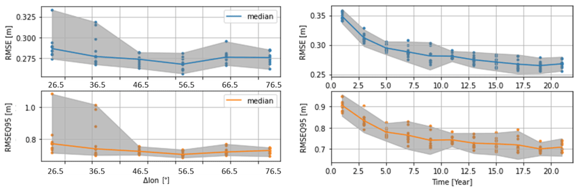
Figure 9RMSE and RMSEQ95 versus Δlongitude (left). RMSE and RMSEQ95 function of Δtime (right).
The plot in Fig. 9 (top left panel) shows that the accuracy of the prediction does not improve by taking winds located at more than 50∘ longitude, which corresponds approximately to the longitude of Saint Pierre and Miquelon. The error increases even after this distance; points that are too far away bring more noise than information, which degrades the prediction.
In the second figure, one can observe that the prediction improves by increasing the learning period. However, a few years are enough to obtain sufficiently accurate predictions (RMSE less than 30 cm, with 5 years of training). Moreover, the slope of the RMSE curve becomes less steep after about 10 years. The considered learning period must also be long enough to cover the variations in the ocean–atmosphere regime over the region. Concerning the Bay of Biscay, 10 years seems to be a sufficient period to observe positive or negative North Atlantic Oscillation (NAO) phases.
5.1 Methods
The two methods used for the comparison were developed by our team and use the previously introduced predictors.
Table 2Scores of Hs prediction by the three methods at node no. 7818.

5.1.1 Analog method
The analog method, originally introduced by Lorenz (1969), is a classical and simple statistical downscaling method that performs, in general, as well as the more complicated methods (Zorita and von Storch, 1999). The recent proliferation of data in atmospheric and oceanographic sciences has strengthened the scientific interest in this method (see, e.g., Platzer et al., 2021 and references therein).
The proposed method is composed of the following four main steps:
-
Dimensionality reduction. The global predictor is composed of more than 5000 points. In a space of this size, it is difficult to find a metric to identify the good analogues due to the curse of dimensionality. Moreover, working in this space would generate too high a computational cost. For these reasons, it is necessary to reduce the dimensionality of the data. The chosen reduction method is the principal component analysis (PCA or EOF, the empirical orthogonal function). This method projects the data onto an orthonormal base in which different individual dimensions are linearly uncorrelated (Jolliffe and Cadima, 2016). Here, only the first 50 principal components are retained, which corresponds to a reduction in dimension by a factor of over 100.
The dissipation of wave energy over long distances is difficult to quantify, but some research show that swells can lose a significant part of their energy (65 % over 2800 km; Ardhuin et al., 2009). To consider the decreasing influence of wind with distance to the target location, a Gaussian kernel is applied to the global predictor before the PCA. The radius of the Gaussian kernel determined after optimization is α=600 km. This distance is very small (points beyond Ireland have weights close to 0). This surprising result is certainly explained by the fact that observing the weather systems that reach the area near the target location provides sufficient information on their history, and that this operation reduces the dimensionality of the data, which favors the search of good analogues.
-
Search for analogs. The search for the nearest neighbors is done using a classical ball tree algorithm (Omohundro, 1989). The distance dk computed is the L2 norm in the PCA space. The nearest neighbors in the sense of this distance are considered as the analogous situations. The 30 nearest neighbors are kept.
-
Prediction. Once the nearest neighbors are identified, the prediction is obtained by averaging the Hs of the analogs weighted by the inverse of the predictor distance.
-
Regression on the residuals. The previous prediction considers only the global wind. To consider the local wind, a multiple linear regression (MLR) is performed on the residuals of the previous prediction over a 2-year test period. The explanatory variables are as follows:
-
Local predictor – local wind
-
– weighted mean of analogues Hs
-
Mean distance to neighbors – the further away from the nearest neighbors, the greater the correction to be applied.
Finally, Hs is determined by the sum between and the MLR output.
-
5.1.2 Linear regression model
The second model compared with HCNN is a linear regression model (Obakrim et al., 2022).
Parameters βg are determined by penalized regression and are sought to be as smooth as possible. Physically, this means that close locations should have close coefficients.
5.2 Results of the three methods
Both models were evaluated on the station presented in the previous section. The results of the three statistical downscaling methods are summarized in Table 2.
The HCNN method gives better results for the four selected indicators. Next comes the linear regression and then the analog method. It should be noted, however, that while the HCNN method outperforms the linear model, it is much less interpretable. There is a tradeoff between interpretability and performance. The analog method, even if it is the conceptually simplest of the three, obtains performances quite close to the linear model.
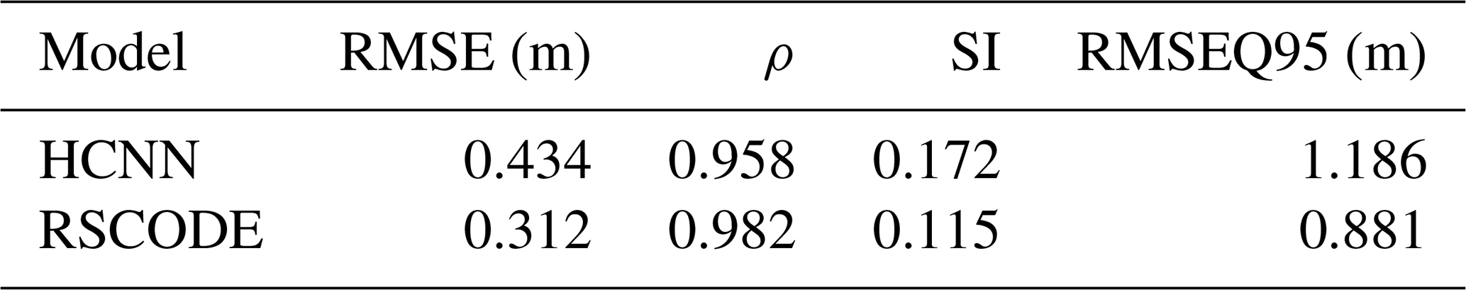
Table 3Scores of Hs prediction by HCNN at station no. 62001. Buoy Hs is taken as the reference.

In the previous sections, the HCNN neural network was only trained on the outputs of the HOMERE numerical model. It is also interesting to evaluate the ability of the network to learn from in situ data. Here, the reference data are from station no. 62001 (https://www.ndbc.noaa.gov/station_page.php?station=62001, last access: 5 October 2021), which is located at the bottom of the continental slope in the Bay of Biscay (45.2∘ N, 5∘ W). The data were collected via the Copernicus Marine In Situ Thematic Assembly Centre (http://www.marineinsitu.eu/dashboard/, last access: 5 October 2021). The depth is more than 4500 m. This buoy is owned and maintained by the UK Met Office in cooperation with Météo-France. As this buoy is located outside the HOMERE mesh, but within the RSCODE mesh, the latter dataset is used to evaluate HCNN.
The waves are, on average, higher than for the previous station (mean of 2.43 m; min 0.20 m and max 11.75 m).
The selected train and test periods are as follows:
-
Train – 29 July 1998 to 31 December 2013 (size of 41 696)
-
Test – 1 January 2014 to 31 December 2016 (size of 8541).
According to Table 3 and Fig. 10, the prediction made by RSCODE is closer to the Hs values measured by the buoy. Moreover, the dispersion around the identity line is less pronounced, and the distribution seems to be better reproduced. Although the HCNN model performs worse for the four scores, its performances nevertheless remain satisfactory, and the prediction of Hs by this model is closer to the buoy than RSCODE in 36 % of the cases.
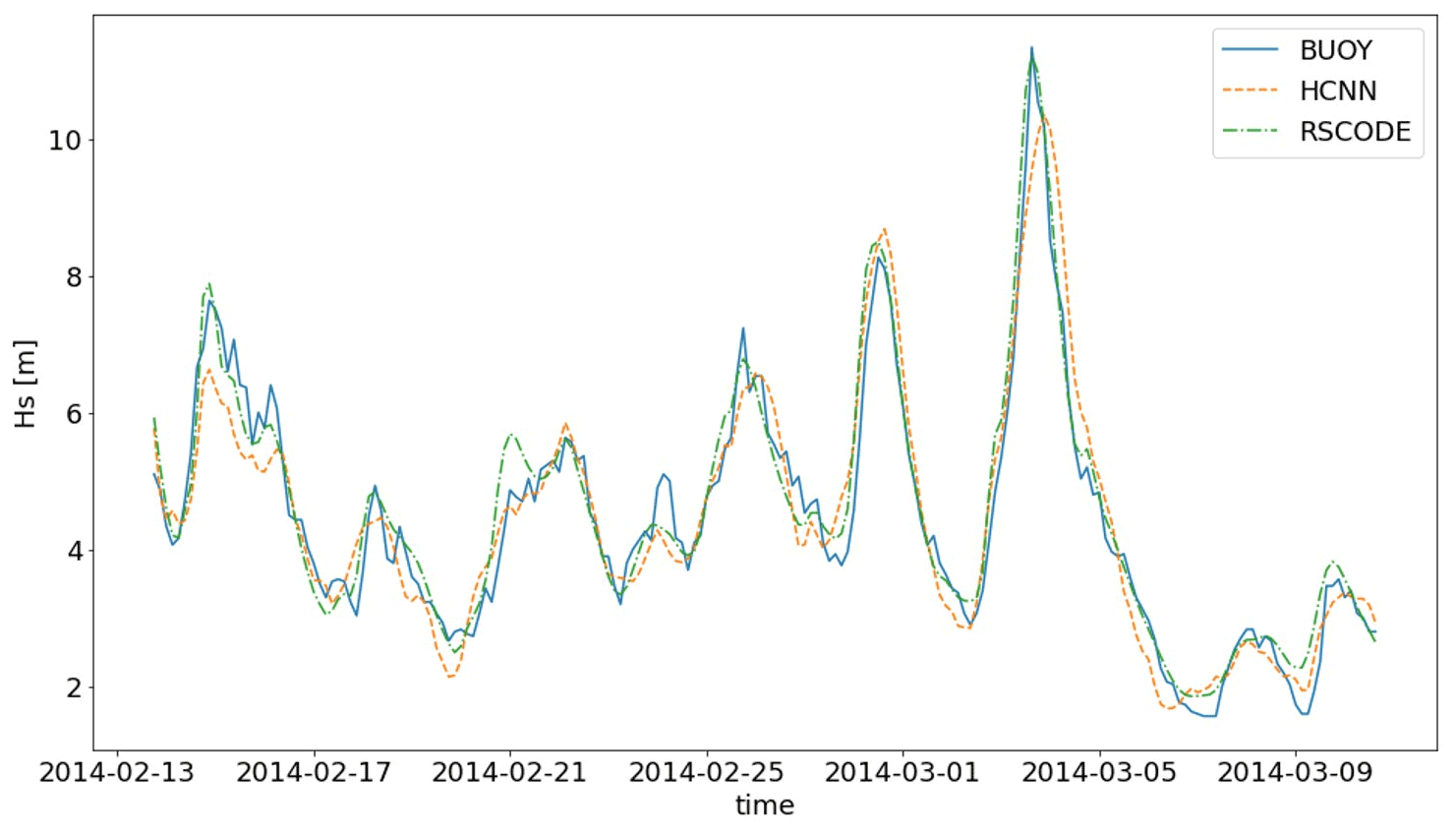
Figure 11A 3 h time series of Hs from the buoy (blue; solid line), HCNN (orange; dashed line), and RSCODE (green; dash-dotted line) at station no. 62001 over 1 month of the validation period.
In Fig. 11, one can notice the smoothness of the prediction of Hs by HCNN. Looking at the three time series, it also appears that the Hs from the buoy is noisier than the Hs from numerical models. The direct consequence is that learning is more complicated with these data. As a comparison, when the training is performed on RSCODE Hs, the scatter index is equal to 0.145.
The deep learning model presented in this study achieves good performance in predicting local sea states from local and global winds. These results once again prove the suitability of these approaches for statistical downscaling problems. The HCNN model even outperforms the other two statistical downscaling methods studied. However, this performance comes at the cost of interpretability. Numerical models remain better than statistical downscaling methods in terms of accuracy, but this result is not sufficient to conclude on the interest of the latter. Indeed, unlike numerical models, the prediction of Hs by these methods is almost instantaneous, and the training of the model requires only a few minutes. Statistical downscaling methods do not require fine tuning of the parameters as is the case for physical models. These advantages, added to the reasonable accuracy of their prediction, make them interesting tools for the prediction of sea states.
Many perspectives remain open for the development of this model. First, we have so far been limited to predicting the significant wave height at a station. Since the global predictor is being defined on a large scale, it remains valid near the target location (the distance of validity remains to be defined), and thus, the prediction could be extended to the neighboring points by varying only the local predictor. Then, it is understood that the method should be able to consider the tidal currents and the variation in the water height to be applied in coastal environment. This point deserves further study and has not been conducted here to focus on the comparison with other models. Finally, the low computational cost makes it possible to use ensemble weather forecasts to predict the significant wave height and a confidence interval, thus reinforcing the value of the prediction made and its usability for marine applications. The proposed methodology could be useful to extend the available history of sea state conditions at locations where such information is sparse. For example, one could be interested in estimating the energy producible by a WEC (Payne et al., 2021) or estimating weather windows for the operation and maintenance of offshore structures (Walker et al., 2013).
Python scripts and data used in Sect. 4 are available online at https://doi.org/10.5281/zenodo.5524370 (Michel et al., 2021).
SO proposed the project of using DL to predict Hs and did the preliminary analyses with projected winds. MM developed the Python codes and all the analysis, along with the oceanographic interpretation of the results. NR eased the access to the dataset and helped with the workflow. VM and PA brought expert advice on neural networks. VM, PA, and NR provided ideas for the development of the method. MM wrote the paper and all co-authors contributed.
The contact author has declared that neither they nor their co-authors have any competing interests.
Publisher's note: Copernicus Publications remains neutral with regard to jurisdictional claims in published maps and institutional affiliations.
The authors acknowledge the two anonymous reviewers, for their numerous and very useful comments and suggestions.
This paper was edited by William Hsieh and reviewed by two anonymous referees.
Anderson, G., Carse, F., Turton, J., and Saulter, A.: Quantification of wave measurements from lightvessels, J. Oper. Oceanogr., 9, 93–102, https://doi.org/10.1080/1755876X.2016.1239242, 2016.
Ardhuin, F.: Ocean waves in geosciences, Technical Report, https://doi.org/10.13140/RG.2.2.16019.78888/5, 2021.
Ardhuin, F., Chapron, B., and Collard, F.: Observation of swell dissipation across oceans, Geophys. Res. Lett., 36, 1–5, https://doi.org/10.1029/2008GL037030, 2009.
Ardhuin, F., Stopa, J. E., Chapron, B., Collard, F., Husson, R., Jensen, R. E., Johannessen, J., Mouche, A., Passaro, M., Quartly, G. D., Swail, V., and Young, I.: Observing Sea States, Front. Mar. Sci., 6, 124, https://doi.org/10.3389/fmars.2019.00124, 2019.
Baño-Medina, J., Manzanas, R., and Gutiérrez, J. M.: Configuration and intercomparison of deep learning neural models for statistical downscaling, Geosci. Model Dev., 13, 2109–2124, https://doi.org/10.5194/gmd-13-2109-2020, 2020.
Boudière, E., Maisondieu, C., Ardhuin, F., Accensi, M., Pineau-Guillou, L. and Lepesqueur, J.: A suitable metocean hindcast database for the design of marine energy converters, International Journal of Marine Energy, 3–4, e40–e52, https://doi.org/10.1016/j.ijome.2013.11.010, 2013.
Camus, P., Mendez, F., Losada, I. J., Menendez, M., Espejo, A., Perez, J., Zamora, A. R., and Guanche, Y.: A method for finding the optimal predictor indices for local wave climate conditions, Ocean Dynam., 64, 1025–1038, https://doi.org/10.1007/s10236-014-0737-2, 2014.
Ewans, K. and Jonathan, P.: Evaluating Environmental Joint Extremes for the Offshore Industry, J. Marine Syst., 130, 124–130, https://doi.org/10.48550/arXiv.1211.1365, 2012.
Gagne II, D. J., Haupt, S. E., Nychka, D. W. and Thompson, G.: Interpretable deep learning for spatial analysis of severe hailstorms, Mon. Weather Rev., 147, 2827–2845, https://doi.org/10.1175/MWR-D-18-0316.1, 2019.
Idier, D., Rohmer, J., Pedredros, R., Le Roy, S., Lambert, J., Louisor, J., Le Cozannet, G., and Le Cornec, E.: Coastal food: a composite method for past events characterisation providing insights in past, present and future hazards – joining historical, statistical and modelling approaches, Nat. Hazards, 101, 465–501, https://doi.org/10.1007/s11069-020-03882-4, 2020.
Jolliffe, I. T. and Cadima, J.: Principal component analysis: a review and recent developments, Philos. T. R. Soc. A, 374, https://doi.org/10.1098/rsta.2015.0202, 2016.
Kingma, D. P. and Ba, J.: Adam: A Method for Stochastic Optimization, International Conference for Learning Representations, arXiv [preprint], arXiv:1412.6980, 2015.
Laugel, A., Menendez, M., Benoit, M., Mattarolo, G., and Mendez, F.: Wave climate projections along the French coastline: Dynamical versus statistical downscaling methods, Ocean Model., 84, 35–50, https://doi.org/10.1016/j.ocemod.2014.09.002, 2014.
Lazure, P. and Dumas, F.: An external–internal mode coupling for a 3D hydrodynamical model for applications at regional scale (MARS), ScienceDirect, Adv. Water Ressour., 31, 233–250, https://doi.org/10.1016/j.advwatres.2007.06.010, 2007.
Lorenz, E. N.: Atmospheric predictability as revealed by naturally occurring analogues, J. Atmos. Sci., 26, 636–646, https://doi.org/10.1175/1520-0469(1969)26<636:APARBN>2.0.CO;2, 1969.
Maisondieu, C.: On the distribution of complex sea-states in the Bay of Biscay, Proceedings of the 12th European Wave and Tidal Energy Conference, Cork, https://www.researchgate.net/publication/319464930_On_the_distribution_of_complex_sea-states_in_the_Bay_of_Biscay (last access: 6 October 2021), 2017.
Michel, M., Obakrim, S., Raillard, N., Ailliot, P., and Monbet, V.: Deep learning for statistical downscaling of sea states – Data and code, Zenodo [data set and code], https://doi.org/10.5281/zenodo.5524370, 2021.
Mouton, C., Myburgh, J. C., and Davel, M. H.: Stride and Translation Invariance in CNNs, Communications in Computer and Information Science, Springer, https://doi.org/10.1007/978-3-030-66151-9_17, 2020.
Obakrim, S., Ailliot, P., Monbet, V., and Raillard, N.: Statistical modeling of the space-time relation between wind and significant wave height, J. Geophys. Res.-Oceans, https://doi.org/10.1002/essoar.10510147.2, 2022.
Omohundro, S. M.: Five Balltree Construction Algorithms, Technical Report, ICSI Technical Report TR-89-063, http://www.icsi.berkeley.edu/ftp/global/pub/techreports/1989/tr-89-063.pdf (last access: 1 April 2022), 1989.
Payne, G., Pascal, R., Babarit, A., and Perignon, Y.: Impact of Wave Resource Description on WEC Energy Production Estimates, Proceedings of the 11th European Wave and Tidal Energy Conference, 5–9 September 2021, Plymouth, UK, 2021.
Pérez, J., Méndez, F. J., Menéndez, M., and Losada, I. J.: ESTELA: a method for evaluating the source and travel time of the wave energy reaching a local area, Ocean Dynam., 64, 1181–1191, https://doi.org/10.1007/s10236-014-0740-7, 2014.
Platzer, P., Yiou, P., Naveau, P., Tandeo, P., Zhen, Y., Ailliot, P., and Filipot, J. F.: Using local dynamics to explain analog forecasting of chaotic systems, J. Atmos. Sci., 78, 2117–2133, https://doi.org/10.1175/JAS-D-20-0204.1, 2021.
Reichstein, M., Camps-Valls, G., Stevens, B., Jung, M., Denzler, J., Carvalhais, N., and Prabhat: Deep learning and process understanding for data-driven Earth system science, Nature, 566, 195–204, https://doi.org/10.1038/s41586-019-0912-1, 2019.
Roland, A. and Ardhuin, F.: On the developments of spectral wave models: numerics and parametrization for the coastal ocean, Ocean Dynam., 64, 833–846, https://doi.org/10.1007/s10236-014-0711-z, 2014.
Saha, S., Moorthi, S., Pan, H., Wu, X., Wang, J., Nadiga, S., Tripp, P., Kistler, R., Woollen, J., Behringer, D., Liu, H., Stokes, D., Grumbine, R., Gayno, G., Wang, J., Hou, Y., Chuang, H., Juang, H. H., Sela, J., Iredell, M., Treadon, R., Kleist, D., Van Delst, P., Keyser, D., Derber, J., Ek, M., Meng, J., Wei, H., Yang, R., Lord, S., van den Dool, H., Kumar, A., Wang, W., Long, C., Chelliah, M., Xue, Y., Huang, B., Schemm, J., Ebisuzaki, W., Lin, R., Xie, P., Chen, M., Zhou, S., Higgins, W., Zou, C., Liu, Q., Chen, Y., Han, Y., Cucurull, L., Reynolds, R. W., Rutledge, G., and Goldberg, M. The NCEP Climate Forecast System Reanalysis, B. Am. Meteorol. Soc., 91, 1015–1057, https://doi.org/10.1175/2010BAMS3001.1, 2010.
Shanker, M., Hu, M. Y., and Hung, M. S.: Effect of data standardization on neural network training, Omega, 24, 385–397, https://doi.org/10.1016/0305-0483(96)00010-2, 1996.
Thomas, J. T. and Dwarakish, G. S.: Numerical Wave Modelling – A Review, Aquatic Procedia, 4, 443–448, https://doi.org/10.1016/j.aqpro.2015.02.059, 2015.
Tracy, B., Devaliere, E. M., Nicolini, T., Tolman, H. L., and Hanson, J. L.: Wind sea and swell delineation for numerical wave modeling, Proc. 10th international workshop on wave hindcasting and forecasting and coastal hazards symposium, JCOMM Tech. Rep. 41, WMO/TD-No. 1442, 2007.
Trzaska, S. and Schnarr, E.: A review of downscaling methods for climate change projections, Technical Report https://www.researchgate.net/publication/267097515_A_Review_of_Downscaling_Methods_for_Climate_Change_Projections (last access: 4 April 2022), 2014.
Walker, R. T, Nieuwkoop, J., Johanning, L., and Parkinson, R.: Calculating weather windows: Application to transit, installation and the implications on deployment success, Ocean Eng., 68, 88–101, https://doi.org/10.1016/j.oceaneng.2013.04.015, 2013.
Wang, X. L., Swail, V. R., and Cox, V. R.: Dynamical versus statistical downscaling methods for ocean wave heights, Int. J. Climatol., 30, 317–332, https://doi.org/10.1002/joc.1899, 2010.
Zorita, E. and von Storch, H.: The Analog Method as a Simple Statistical Downscaling Technique: Comparison with More Complicated Methods, J. Climate, 12, 2474–2489, https://doi.org/10.1175/1520-0442(1999)012<2474:TAMAAS>2.0.CO;2, 1999.
- Abstract
- Introduction
- Data
- Presentation of the method
- Evaluation of the method in the Bay of Biscay
- Comparison of statistical downscaling methods
- Application to in situ data and comparison with RSCODE
- Conclusions and perspectives
- Code and data availability
- Author contributions
- Competing interests
- Disclaimer
- Acknowledgements
- Review statement
- References