Spatial patterns and indices for heat waves and droughts over Europe using a decomposition of extremal dependency

We present a method for the analysis and compact description of large-scale multivariate weather extremes. Spatial patterns of extreme events are identified using the tail pairwise dependence matrix (TPDM) proposed by Cooley and Thibaud (2019). We also introduce the cross-TPDM to identify patterns of common extremes in two variables. An extremal pattern index (EPI) is developed to provide a pattern-based aggregation of temperature. A heat wave definition based on EPI is able to detect the most important heat waves over Europe. As an extension for considering simultaneous extremes in two variables, we propose the threshold-based EPI (TEPI) that captures the compound character of spatial extremes. We investigate daily temperature maxima and precipitation deficits at different accumulation times and find evidence that preceding precipitation deficits have a significant influence on the development of heat waves and that heat waves often co-occur with short-term drought conditions. We exemplarily show for the European heat waves of 2003 and 2010 that TEPI is suitable for describing the large-scale compound character of heat waves.

1 Introduction

Extreme weather events over Europe, such as heat waves and droughts, but also heavy rainfall events have repeatedly attracted attention in recent years due to their dramatically high impact on socioeconomic systems. The most prominent European heat waves in the 21st century occurred in 2003, 2010, and 2018. The high temperatures, which lasted for a period of several weeks to months, in combination with compound drought periods, led to disastrous effects on socioeconomic and local natural systems, such as an increased number of wildfires, crop failure, and increased health-related deaths (see, e.g.,  Liu et al., 2020; Fischer and Schär, 2010). For instance, according to WHO, more than 70 000 additional deaths in 12 European countries can be attributed to the European heat wave in 2003 (Anderson et al., 2004), which was very likely the hottest summer in 500 years (Luterbacher et al., 2004).

Several studies indicate that an increase in the global mean temperature and its variability leads to more frequent heat wave and drought events that are characterized by longer durations and greater severity (Gershunov and Douville, 2009; Dai et al., 2018; Guerreiro et al., 2018; Della-Marta et al., 2007). This is also confirmed in the recent IPCC report (IPCC, 2021), saying that European hot extremes (including heat wave) have significantly increased in intensity and number since 1950. Particularly severe heat waves in Europe occurred in recent years in 2018, 2019, and 2022, often in connection with drought conditions. The 2022 heat wave resulted in record-breaking temperatures in France, Spain, the United Kingdom, and Germany (Rousi et al., 2023). Our understanding of the underlying dynamics of heat waves and, consequently, the changes that can be expected under climate change have improved considerably in recent years. In contrast, the dynamics and underlying structure of co-occurring temperature and drought events are much less understood. However, studies show that concurrent drought events can strongly influence heat extremes (Zscheischler and Seneviratne, 2017). For example, for the heat wave of 2003, it has been demonstrated that the co-occurring drought was a key contributor to the extreme temperature anomalies (e.g.,  Fischer et al., 2007; Black et al., 2004; Ferranti and Viterbo, 2006). Therefore, when considering potential changes under climate change, joint consideration of heat and drought extremes is necessary.

Several definitions and indices for drought and heat waves can be found in the literature. Heat wave indices usually include daily maximum temperature exceeding a certain threshold for several consecutive days (Robinson, 2001). Standard indices for heat waves are, e.g., the heat and cold wave index (HCWI) (Lavaysse et al., 2018), which is implemented in the Copernicus European Drought Observatory or the heat wave duration index (HWDI) and has been recommended by the IPCC (Griggs and Noguer, 2002). Standard meteorological drought indices are, e.g., the Palmer drought severity index (PDSI) (Palmer, 1965) and the standardized precipitation index (PSI) (McKee et al., 1993). A recent, promising approach to identifying heat waves and droughts is presented by Schädler and Breil (2021). They base their evaluation on so-called regional climate networks (RCNs) and identify extremes over Germany. Indices for compound heat waves and drought are less common in the literature. Recent approaches to index definition include the dry-hot magnitude index (Wu et al., 2019) or the standardized compound event indicator (Hao et al., 2019).

Detection and attribution (D&A) provides a powerful statistical tool for analyzing climate change's complex causes and effects. Reviews of the application of D&A to meteorological data are given in Slater et al. (2021) and Ummenhofer and Meehl (2017). In the high-dimensional space of the climate system, both the natural variability of the system and some internal variability overshadow the signals of climate change (Fischer and Knutti, 2016). Therefore, local changes, especially on smaller scales, only become visible if the data are analyzed in a compressed form. Data compression is therefore of great importance for a successful and reliable D&A study.

There exists a variety of statistical methods of different complexity for information compression. For example, a relatively simple approach is to aggregate the data spatially, but this usually neglects the spatial dependence structure of the underlying extreme values. Other techniques may include filtering using Fourier or wavelet transforms or adaptive data methods such as principal component analysis (PCA). However, most data compression methods focus on the description of the bulk of the underlying distribution, as described by first- and second-order moments, and provide little to no information about the tail of the distribution. Adaptive data methods have been widely used to study the spatial structure of heat waves. For example, Stefanon et al. (2012) use a clustering approach to identify six common heat wave patterns over Europe. Schubert et al. (2014) identify and analyze spatial patterns related to precipitation and temperature based on rotated empirical orthogonal functions (EOFs) over Russia. The studies agree that the patterns identified are consistent with large-scale blocking anticyclones associated with Rossby waves.

For the D&A of extreme events, mathematical methods are needed that achieve a targeted description of extremes. The framework in which these methods operate is the multivariate extreme value theory (MEVT) with broad applications in mathematical and meteorological research (e.g., Beirlant et al., 2006; Coles et al., 2001). New approaches combine MEVT with existing information compression methods. The rich experience with these methods in atmospheric research allows their targeted application to extreme events. For example, Morris et al. (2019) use an approach based on empirical basis functions to model the spatial dependence of low-rank max-stable processes. Janßen and Wan (2020) and Saunders et al. (2021) propose clustering approaches combined with an extremal framework, and Goix et al. (2017) also use a clustering approach to design a statistical learning procedure for anomaly detection based on a dataset with standard Pareto margins. Boulaguiem et al. (2022) combine generative adversarial networks with extreme value theory to model spatial dependencies in temperature and precipitation extremes. This shows that some of these methods are suitable for the description of composite extrema in two variables. For example, Vignotto et al. (2021) use an extreme value dependence clustering approach to identify spatial patterns of situations where precipitation and wind extremes are very likely to occur simultaneously.

Another promising approach comes from Cooley and Thibaud (2019). They propose the tail pairwise dependence matrix (TPDM), which summarizes extremal dependence using a regular varying framework and a threshold-based estimator. They build on the work of Larsson and Resnick (2012), who first defined this matrix for the bivariate case and show that the TPDM has some favorable properties that it shares with the covariance matrix so that the TPDM can be used as an analog to the covariance matrix for extremes. Jiang et al. (2020) and Rohrbeck and Cooley (2023) propose a PCA study using the TPDM with applications to daily precipitation over the United States (Jiang et al., 2020) as well as historical river flow levels across northern England and southern Scotland (Rohrbeck and Cooley, 2023). Drees and Sabourin (2019) also investigate a PCA based on the TPDM but focus more on describing the mathematical background. Finally, Fix et al. (2021) use the TPDM to propose a new model for spatial dependencies inspired by the simultaneous autoregressive (SAR) model with application to a gridded dataset of daily precipitation over Colorado.

In this paper, we introduce the extremal pattern index (EPI) for spatial weather extremes. The EPI is constructed based on the leading patterns derived from a PCA for extremes, as proposed by Jiang et al. (2020). Climate indices based on PCA, e.g., for the North Atlantic Oscillation (Barnston and Livezey, 1987), are already well-established tools in climate monitoring and analysis. By replacing the covariance matrix with the TPDM, we shift our focus to identifying extreme weather patterns, such as heat waves and droughts, while leaving the PCA procedure basically unchanged.

We use daily maximum 2 m temperature (maxT2m) from COSMO-REA6 reanalysis to derive the TPDM and identify spatial patterns associated with temperature extremes. Its EPI describes the intensity and spatial extent of heat waves in the area under consideration. To test the suitability of the EPI for describing heat waves, we focus on the two European heat waves in 2003 and 2010, about which many publications already exist. We compare our findings with existing literature.

We further explore the potential use and benefits of the TPDM in describing co-occurring heat waves and meteorological droughts. We again use maxT2m and define precipitation deficit (PD) as the additive reciprocal of daily precipitation accumulated over periods ranging from 11 to 47 d. To identify the pairwise extremal dependence between both variables, we introduce the cross-TPDM and provide an estimator thereof. We decompose the estimator of the cross-TPDM using a singular value decomposition (SVD), providing insight into the co-occurrence of extreme spatial patterns in two variables. Finally, we apply an analogue definition of the EPI using the SVD of the cross-TPDM. In order to target the index to co-occurring events, a modulated threshold-based estimator of EPI (TEPI) is defined.

The remainder of the paper is organized as follows. First, the theoretical framework of regular variation underlying the definition of the TPDM is presented in Sect. 2. Here we also discuss the estimation of the TPDM and its decomposition. Accordingly, we introduce the cross-TPDM in Sect. 3. We then discuss their evaluation (Sect. 4) and the definition of the various extremal pattern indices (Sect. 5). Section 6 discusses the data and some pre-processing steps. The results are presented in Sect. 7 with a discussion first on the temperature extremes and the EPI to define heat waves and then the compound heat wave and drought events. The paper concludes with a summary and discussion in Sect. 8.

2 The tail pairwise dependence matrix (TPDM)

2.1 Definition of the TPDM

The definition of the TPDM is based on regularly varying random variables. Regularly varying variables are defined by the tail behavior of their distribution function F(x) in the limit x→∞. A summary on regular variation is given by Resnick (2007) saying “regularly varying functions are those functions which behave asymptotically like power functions”. Let X be a non-negative random variable with positive and measurable distribution function F(x) on ℝ₊. We call F to be a regularly varying function with tail index ρ∈ℝ (denoted by F(X)∈RV_ρ), if for all t>0

$$\begin{array}{}\text{(1)}& \underset{x\to \mathrm{\infty }}{lim}{\displaystyle \frac{F\left(xt\right)}{F\left(x\right)}}=t^{\mathit{\rho }}.\end{array}$$

If the tail function, $\stackrel{\mathrm{‾}}{F}\left(X\right)=\mathrm{1}-F\left(X\right)$, is a regularly varying function, i.e. $\stackrel{\mathrm{‾}}{F}\left(X\right)\in R{V}_{-\mathit{\rho }}$ (ρ>0), then X is a regularly varying random variable with tail index ρ (Resnick, 2007, Theorem 3.6), and we write X∈RV_ρ. If X is Fréchet-distributed with $F\left(x\right)=\exp (-x^{-\mathit{\alpha }})$ and x≥0, then X is a regularly varying random variable with tail index α (Resnick, 2007).

Now let X be a positive multivariate random variable of dimension p with Fréchet-distributed margins and tail index α. In the following, we denote $X\in R{V}_{\mathit{\alpha }}^{+}$. For multivariate regularly varying random variables, it is convenient to transform the random vector to generalized polar coordinates with the angular component ω and the radial component r. With any norm $\left|\right|\cdot \left|\right|$ we define the unit sphere ${\mathbb{S}}_{+}^{p-\mathrm{1}}$ as

$$\begin{array}{}\text{(2)}& {\mathbb{S}}_{+}^{p-\mathrm{1}}=\left\{x\in {\mathbb{R}}_{+}^p:\left|\right|x\left|\right|=\mathrm{1}\right\}\end{array}$$

and the polar coordinate transform as

$$\begin{array}{}\text{(3)}& x\to \left(\left|\right|x\left|\right|,{\displaystyle \frac{x}{\left|\right|x\left|\right|}}\right)=:(r,\mathit{\omega })\text{ for }\left|\right|x\left|\right|>\mathrm{0},\end{array}$$

with $r=\left|\right|x\left|\right|$ and $\mathit{\omega }=x/\left|\right|x\left|\right|$. If X is regularly varying, then its radial and angular components become conditionally independent for r→∞.

To understand the derivation and definition of the TPDM, we explore the properties of a regularly varying random variable. This exploration is done through the lens of weak convergence (Resnick, 2007), restricted to the special case of vague convergence, denoting convergence of Radon measures. Given a multivariate, Fréchet-distributed random vector $X\in R{V}_{\mathit{\alpha }}^{+}$, the definition of regular variation says that there is a sequence b_n with n→∞ and a limit measure ν(⋅), such that we can write $n\mathbb{P}[X/b_n\in \cdot ]\stackrel{\mathit{\nu }}{⟶}\mathit{\nu }(\cdot )$ as n→∞. Here, $\stackrel{\mathit{\nu }}{⟶}$ denotes vague convergence in $M_{+}\left(\right[\mathrm{0},\mathrm{\infty }{]}^p\setminus \mathit{\left\{}\mathrm{0}\mathit{\right\}})$, the space of Radon measures on $(\mathrm{0},\mathrm{\infty }]\setminus \mathit{\left\{}\mathrm{0}\mathit{\right\}}$. After the polar transform, one can specify $\mathit{\nu }(\mathrm{d}r\times \mathrm{d}\mathit{\omega })=\mathit{\rho }{r}^{-\mathit{\rho }-\mathrm{1}}\mathrm{d}r\mathrm{d}H\left(\mathit{\omega }\right)$ where ρ is the tail index of X, and H is some Radon measure, referred to as the angular measure on ${\mathbb{S}}_{+}^{p-\mathrm{1}}$. It can be interpreted as a probability measure for ω (for a detailed description see, e.g.,  Larsson and Resnick, 2012; Cooley and Thibaud, 2019; Resnick, 2007).

Larsson and Resnick (2012) found that the measure H, on the unit sphere ${\mathbb{S}}_{+}^{p-\mathrm{1}}$, holds information about extremal dependencies. They define the extremal dependence measure of any regularly varying, bivariate random vector based on its angular components after polar transformation.

Cooley and Thibaud (2019) expand the original approach to higher dimensions. They concentrate on Fréchet-distributed variables with tail index α=2 and choose the L₂ norm when transforming into polar coordinates. They define the tailed pairwise dependence between the ith and jth element of X, using its angular component ω as

$$\begin{array}{}\text{(4)}& {\mathit{\sigma }}_{ij}=\underset{{\mathbb{S}}_{+}^{p-\mathrm{1}}}{\int }{\mathit{\omega }}_i{\mathit{\omega }}_j\mathrm{d}H\left(\mathit{\omega }\right).\end{array}$$

The TPDM (Σ_X) is then a p×p matrix, which summarizes the pairwise extremal dependencies of X for all margins $i,j=\mathrm{1},\mathrm{\dots },p$: ${\mathrm{\Sigma }}_X=({\mathit{\sigma }}_{ij}{)}_{i,j=\mathrm{1}\mathrm{\dots }p}$. Cooley and Thibaud (2019) show that by their choice of parameters, the properties of the TPDM are very close to those of the covariance matrix. The most important property for our application is that the TPDM is symmetric and positive definite with real and positive eigenvalues. For rigorous derivations and proofs as well as additional literature, the reader is referred to Cooley and Thibaud (2019).

2.2 Estimation of the TPDM

Let x_t, $t=\mathrm{1},\mathrm{\dots },n$ be a sample of a p-dimensional random vector X with Fréchet margins and sample components $x_{t,i},i=\mathrm{1},\mathrm{\dots },p$. The estimator of the individual elements of the TPDM is given by Jiang et al. (2020) as

$$\begin{array}{}\text{(5)}& {\widehat{\mathit{\sigma }}}_{ij}=\mathrm{2}{n}_{ij,\mathrm{exc}}^{-\mathrm{1}}\sum _{t=\mathrm{1}}^n{w}_{t,i}{w}_{t,j}{\mathbb{I}}_{(r_{t,ij}>r_{\mathrm{0},ij})}.\end{array}$$

with $r_{t,ij}=\sqrt{x_{t,i}^{\mathrm{2}}+x_{t,j}^{\mathrm{2}}}$ as well as $w_{t,i}=x_{t,i}/r_{t,ij}$ and $w_{t,j}=x_{t,j}/r_{t,ij}$. r_0,ij is a threshold that can be set individually, with the index function 𝕀 ensuring that only observations larger than r_0,ij are considered for the estimation, and $n_{ij,\mathrm{exc}}={\sum }_{t=\mathrm{1}}^n{\mathbb{I}}_{(r_{t,ij}>r_{\mathrm{0},ij})}$ is the number of elements which are greater than r_0,ij. The positive definiteness of the TPDM is not guaranteed by the proposed estimator in Eq. (5). If the estimator is not positive definite, we follow Cooley and Thibaud (2019) by computing the nearest correlation matrix (Higham, 2002).

Pre-processing is required when using meteorological data. Again we follow Jiang et al. (2020) and transform the marginal distribution of the original data to Fréchet margins with tail index α=2. Let X^orig be the original random vector with marginal distribution $F_i^{\mathrm{orig}}\left(X\right),i=\mathrm{1},\mathrm{\dots },p$ and X the transformed random vector with Fréchet margins $F_i\left(X\right)=\exp (-x_i^{-\mathit{\alpha }})$. Due to the conservation of probability, we have to ensure that $F_i\left(X\right)=F_i^{\mathrm{orig}}\left(X^{\mathrm{orig}}\right)$, which leads us to the transformation

$$\begin{array}{}\text{(6)}& X_i=(-\log F_i^{\mathrm{orig}}(X^{\mathrm{orig}}){)}^{-\mathrm{1}/\mathit{\alpha }}.\end{array}$$

As an estimator for $F_i^{\mathrm{orig}}$, we may either use the empirical distribution function or fit a parametric distribution (e.g. normal distribution).

2.3 Decomposition of TPDM

The eigenvalue decomposition (EVD) of a covariance matrix is a standard tool in climate data analysis to reduce the dimensionality of high-dimensional weather and climate data (see, e.g., Wallace et al., 1992). The eigenvectors (EVs) form an orthogonal, complete base system. Here we use an estimator based on extreme dependencies instead of covariances, which leads to a targeted consideration of extremal dependencies. For an introduction to EVD and its applications, see, for example, Wilks (2011), Jolliffe (1986), and Björnsson and Venegas (1997). The decomposition of the TPDM, with Σ_XX=UΛU^T, provides the eigenvector matrix U with eigenvectors $u^{\left(k\right)},k=\mathrm{1},\mathrm{\dots },p$ and components $u_{\mathrm{1}}^{\left(k\right)},\mathrm{\dots }{u}_p^{\left(k\right)}$, as well as the diagonal-matrix Λ, containing the eigenvalues λ₁,…λ_p.

The TPDM is defined on the basis of positive real numbers. The transformation to Fréchet margins leads to the input variable X being consistent with this assumption. However, the EVs of the TPDM live by construction in ℝ^p. For the EVs to form an orthogonal basis in ${\mathbb{R}}_{+}^p$, we have to transform the EVs from ℝ^p to ${\mathbb{R}}_{+}^p$. We again follow Cooley and Thibaud (2019) and use $\mathit{\tau }\left(y\right)=\log (\mathrm{1}+\exp (y\left)\right)$ with its back-transform ${\mathit{\tau }}^{-\mathrm{1}}\left(y\right)=\log \left(\exp \right(y)-\mathrm{1})$. The Fréchet distribution, as well as the orthogonality of the EVs, is preserved under this transformation. We transform the EVs component-wise with $e_j^{\left(k\right)}=\mathit{\tau }\left(u_j^{\left(k\right)}\right)$, for each of the $j=\mathrm{1},\mathrm{\dots },p$ components and $k=\mathrm{1},\mathrm{\dots },p$ vectors. The time series of principal components (PCs), in contrast, are calculated by a projection of the back-transformed data X on the respective EV as

$$\begin{array}{}\text{(7)}& \mathit{\eta }=U^T{\mathit{\tau }}^{-\mathrm{1}}\left(X\right).\end{array}$$

We can reconstruct a filtered data set for each sample x_t ($t=\mathrm{1},\mathrm{\dots },n$) of the p-dimensional input variable X using ${\stackrel{\mathrm{̃}}{x}}_t=\mathit{\tau }\left({\mathit{\eta }}_{t}U\right)$.

3 The cross-TPDM

3.1 Definition of the cross-TPDM

The TPDM presented above provides information on the pairwise dependencies between the margins of a random vector. Here we introduce the cross-TPDM as a measure of extremal dependency between two random vectors, such as spatial fields of maxT2m and PD.

Let X and Y be Fréchet random vectors with tail index α and dimensions p and q, respectively. For the following definitions, we consider a joint random vector $Z=(X_{\mathrm{1}},\mathrm{\dots },X_p,Y_{\mathrm{1}},\mathrm{\dots },Y_q{)}^T$ of dimension (p+q). As in Sect. 2, we use the L₂ norm $\left|\right|z\left|\right|$ to define the unit sphere:

$$\begin{array}{}\text{(8)}& {\mathbb{S}}_{+}^{(p+q)-\mathrm{1}}=\mathit{\{}z\in {\mathbb{R}}_{+}^{p+q}:|\left|z\right||=\mathrm{1}\mathit{\}}.\end{array}$$

Along with the transformation of z into polar coordinates,

$$\begin{array}{}\text{(9)}& z\to \left(\left|\right|z\left|\right|,{\displaystyle \frac{z}{\left|\right|z\left|\right|}}\right)=:(r,\mathit{\omega }),\end{array}$$

with $r=\left|\right|z\left|\right|$ and $\mathit{\omega }=z/\left|\right|z\left|\right|$. Following Eq. (4) we define the joint TPDM, which has the dimensions $(p+q)\times (p+q)$. It separates into Σ_XX, Σ_YY, and the cross-TPDM Σ_XY, which is a p×q matrix. If we break down ω into its x and y components ${\mathit{\omega }}^x=(x_{\mathrm{1}}/|\left|z\right||,\mathrm{\dots },x_p/|\left|z\right||{)}^T$ and ${\mathit{\omega }}^y=(y_{\mathrm{1}}/|\left|z\right||,\mathrm{\dots },y_q/|\left|z\right||{)}^T$, the cross-TPDM Σ_XY has the entries

$$\begin{array}{}\text{(10)}& {\mathit{\sigma }}_{ij}=\underset{{\mathbb{S}}_{+}^{(p+q)-\mathrm{1}}}{\int }{\mathit{\omega }}_i^x{\mathit{\omega }}_j^y\mathrm{d}H\left(\mathit{\omega }\right).\end{array}$$

The cross-TPDM is the counterpart of the cross-covariance matrix and represents an extension of the TPDM to two variables. By definition, it is a component of the joint TPDM, obtained from the joint random vector Z. While it is conceivable that the joint TPDM could also be used to extract information about the extremal dependence between X and Y, this approach is relatively rare and involves higher computational costs.

3.2 Estimation of the cross-TPDM

Let x_t, y_t, $t=\mathrm{1},\mathrm{\dots },n$ be samples of two Fréchet random vectors X and Y, with components x_t,i, $i=\mathrm{1},\mathrm{\dots },p$ and y_t,j, $j=\mathrm{1},\mathrm{\dots },q$. To estimate the cross-TPDM, we compute, for the radial component,

$$\begin{array}{}\text{(11)}& r_{t,ij}=\sqrt{x_{t,i}^{\mathrm{2}}+y_{t,j}^{\mathrm{2}}}\end{array}$$

and, for the angular components,

$$\begin{array}{}\text{(12)}& w_{t,i}^x={\displaystyle \frac{x_{t,i}}{r_{t,ij}}};w_{t,j}^y={\displaystyle \frac{y_{t,j}}{r_{t,ij}}}.\end{array}$$

We then estimate each element of the cross-TPDM Σ_XY as

$$\begin{array}{}\text{(13)}& {\widehat{\mathit{\sigma }}}_{ij}=\mathrm{2}{n}_{ij,\mathrm{exc}}^{-\mathrm{1}}\sum _{t=\mathrm{1}}^n{w}_{t,i}^x{w}_{t,j}^y{\mathbb{I}}_{(r_{t,ij}>r_{\mathrm{0},ij})}.\end{array}$$

with threshold r_0,ij and $n_{ij,\mathrm{exc}}={\sum }_{t=\mathrm{1}}^n{\mathbb{I}}_{(r_{t,ij}>r_{\mathrm{0},ij})}$, the number of exceedances.

3.3 Decomposition of the cross-TPDM

The SVD of a cross-covariance matrix is a standard tool in climate data analysis to reduce the dimensionality of high-dimensional weather and climate data (see, e.g.,  Wallace et al., 1992). The singular vectors (SVs) form an orthogonal basis, which can be used for information compression. Here we use an estimator based on extreme dependencies instead of cross-covariances, which leads to a targeted consideration of extremal dependencies. For an introduction to SVD and its applications, see, for example, Wilks (2011), Jolliffe (1986), and Björnsson and Venegas (1997).

The decomposition of the cross-TPDM with Σ_XY=UΛV^T provides left and right singular vectors (SVs), as well as the matrix Λ, which contains the singular values on its diagonal. The SVs can be interpreted as pairs of spatial patterns that explain the maximum possible proportion of extremal dependence, analogous to SVD in Newman and Sardeshmukh (1995). As they point out, one should be cautious in the physical interpretation of the patterns, since they are first of all statistical patterns. However, data reduction based on SVs does not require the physical interpretability of the patterns. The singular values provide information about the extent to which the dependencies are explained by the respective SV patterns.

The cross-TPDM is defined on the basis of positive real numbers. The transformation to Fréchet margins leads to the input variables X and Y being consistent with this assumption. However, the SVs live by construction in ℝ^p. For the SVs to form an orthogonal basis in ${\mathbb{R}}_{+}^p$, we have to transform the SVs from ℝ^p to ${\mathbb{R}}_{+}^p$. We again follow Cooley and Thibaud (2019) and use $\mathit{\tau }\left(y\right)=\log (\mathrm{1}+\exp (y\left)\right)$ with its back-transform ${\mathit{\tau }}^{-\mathrm{1}}\left(y\right)=\log \left(\exp \right(y)-\mathrm{1})$. The Fréchet distribution, as well as the orthogonality of the SVs, is preserved under this transformation. Again, we transform the SVs component-wise. The time series of expansion coefficients (ECs) are calculated by a projection of the back-transformed data X and Y on the respective SVs as

$$\begin{array}{}\text{(14)}& {\displaystyle }\mathit{\eta }=& {\displaystyle }{U}^T{\mathit{\tau }}^{-\mathrm{1}}\left(X\right)\text{(15)}& {\displaystyle }\mathit{\nu }=& {\displaystyle }{V}^T{\mathit{\tau }}^{-\mathrm{1}}\left(Y\right).\end{array}$$

Reconstructions of each sample x_t and y_t ($t=\mathrm{1},\mathrm{\dots },n$) are obtained using ${\stackrel{\mathrm{̃}}{x}}_t=\mathit{\tau }\left({\mathit{\eta }}_{t}U\right)$ and ${\stackrel{\mathrm{̃}}{y}}_t=\mathit{\tau }\left({\mathit{\nu }}_{t}V\right)$.

4 Evaluation

To assess how many EVs or SVs are needed to represent the main features of the data, we use the fraction of explained covariance, which is

$$\begin{array}{}\text{(16)}& {\mathrm{ECF}}_k={\displaystyle \frac{{\mathit{\lambda }}_k}{{\sum }_{i=\mathrm{1}}^p{\mathit{\lambda }}_i}},\end{array}$$

with λ_k the kth largest eigenvalue or singular value in Λ. The term ECF (explained covariance function) in the context of (cross-)TPDM may be misleading because, strictly speaking, SVs no longer provide information about (cross-)covariance but about extremal dependence. Nevertheless, we use the term here because it is a fixed term for measuring the explained dependencies in PCA or SVD.

To examine the extent to which each pattern is dominated by individual events that occurred during the training period and find an appropriate number of modes that yields a representative subset of patterns, we perform 2-fold cross-validation. There are several measurements that aim to find the “optimal” number of modes after PCA (see, e.g.,  Abdi and Williams, 2010). We use $Q_m^{\mathrm{2}}$ as a rather simple but effective measure to assess overfitting (i.e., the point at which the quality of the prediction decreases with an increasing number of modes). To derive $Q_m^{\mathrm{2}}$ we divide the time series into two periods of equal length and calculate a (cross-)TPDM for each period, respectively.

The reconstructions follow Sect. 2.3 and 3.3. The within-sample reconstruction ${\stackrel{\mathrm{̃}}{x}}_t^m=\mathit{\tau }\left({\stackrel{\mathrm{̃}}{u}}^T{\mathit{\tau }}^{-\mathrm{1}}\right(x_t\left)\stackrel{\mathrm{̃}}{u}\right)$ uses the first m EVs/SVs $\stackrel{\mathrm{̃}}{u}$ derived from the period including t, while the out-of-sample reconstruction ${\widehat{x}}_t^m$ uses the corresponding EVs/SVs $\widehat{u}$ of the period not including t. The reconstructions of the two periods are then merged to calculate $Q_m^{\mathrm{2}}$ defined as

$$\begin{array}{}\text{(17)}& Q_m^{\mathrm{2}}=\mathrm{1}-{\displaystyle \frac{{\sum }_{t=\mathrm{1}}^n\left|\right|x_t-{\widehat{x}}_t^m|{|}_{\mathrm{2}}}{{\sum }_{t=\mathrm{1}}^n\left|\right|x_t-{\stackrel{\mathrm{̃}}{x}}_t^{m-\mathrm{1}}|{|}_{\mathrm{2}}}},\end{array}$$

with $\left|\right|\cdot |{|}_{\mathrm{2}}$ the L₂ norm. $Q_m^{\mathrm{2}}$ is a measure of information gain relative to the increase of noise. A positive $Q_m^{\mathrm{2}}$ means that the mth EV/SV mode significantly improves an out-of-sample reconstruction relative to the in-sample reconstruction using m−1 EV/SV modes. The number of modes m at which $Q_m^{\mathrm{2}}$ becomes negative indicates the point at which overfitting starts to occur. The standard error of $Q_m^{\mathrm{2}}$ is assessed by resampling using a block bootstrap method of annual data with 100 samples.

5 Extremal pattern index

We define an extremal pattern index (EPI) based on the PCs using the L₂ norm. The L₂ norm is chosen since both PCA and SVD may be defined as an L₂-minimization problem (see, e.g.,  Abdi and Williams, 2010). Let be given m PCs η_t at time t as derived by Eq. (7) using the m leading EV of a TPDM. We further incorporate the leading eigenvalues/singular values ${\mathit{\lambda }}_{\mathrm{1},\mathrm{\dots },m}$ to normalize the EPI, which we define at time t as

$$\begin{array}{}\text{(18)}& {\mathrm{EPI}}_t^{\mathit{\eta }}={\displaystyle \frac{\sqrt{{\sum }_{k=\mathrm{1}}^m{\mathit{\eta }}_{t,k}^{\mathrm{2}}}}{\sqrt{{\sum }_{j=\mathrm{1}}^m{\mathit{\lambda }}_j}}}.\end{array}$$

The EPI represents a spatial aggregation and shows when individual patterns or a linear combination of patterns are particularly pronounced. The first EV/SVs of the (cross-)TPDM show little spatial variation (see, e.g., Cooley and Thibaud, 2019), so η_t,1 and ν_t,1 essentially represent the spatial mean of the Fréchet-distributed variables. The higher modes are those representing the spatial variation patterns. Thus, the EPI can become extreme even if the first principal component is not outstanding.

The SVD of the cross-TPDM provides two ECs, for the right and the left singular vectors. We define the EPI for the cross-TPDM analogously as

$$\begin{array}{}\text{(19)}& {\mathrm{EPI}}_t^{\mathit{\eta },\mathit{\nu }}={\displaystyle \frac{\sqrt{{\sum }_{k=\mathrm{1}}^m({\mathit{\eta }}_{t,k}^{\mathrm{2}}+{\mathit{\nu }}_{t,k}^{\mathrm{2}})}}{\sqrt{{\sum }_{j=\mathrm{1}}^m{\mathit{\lambda }}_j}}}.\end{array}$$

This definition of EPI describes scenarios where either one or both of the corresponding ECs are high. To account for the simultaneous occurrence of extremes, we introduce a threshold-based approach that considers both the left and right ECs of each mode k to be prominently expressed. We refer to this as the threshold-based extremal pattern index (TEPI).

$$\begin{array}{}\text{(20)}& {\mathrm{TEPI}}_t^{\mathit{\eta },\mathit{\nu }}={\displaystyle \frac{\sqrt{{\sum }_{k=\mathrm{1}}^m({\mathit{\eta }}_{t,k}^{\mathrm{2}}+{\mathit{\nu }}_{t,k}^{\mathrm{2}}){\mathbb{I}}_{\left(\right|{\mathit{\eta }}_{t,k}|>q_{\mathit{\eta }},|{\mathit{\nu }}_{t,k}|>q_{\mathit{\nu }})}}}{\sqrt{{\sum }_{j=\mathrm{1}}^m{\mathit{\lambda }}_j}}},\end{array}$$

with threshold values q_η and q_ν. The threshold ensures that the associated patterns are simultaneously highly pronounced.

6 Application

6.1 Data description

This study relies on the COSMO-REA6 regional reanalysis (Bollmeyer et al., 2015). COSMO-REA6 was developed within the Hans Ertel Centre for Weather Research (HErZ) at the University of Bonn. COSMO-REA6 is currently available for the period from 1995 to 2019 at the opendata FTP server¹ of the German meteorological service (DWD).

We use accumulated PD, as well as daily maxT2m. PD is defined as the additive inverse of precipitation accumulated over various periods between 11 and 47 d using a centered moving-average approach (e.g., for an accumulation period of 11 d, PD is estimated at the center including the 5 d preceding and following the center date, respectively). The use of the moving average for precipitation is less common in the literature, but for our application, we consider it appropriate. Otherwise, we would rather focus on the precipitation deficit before a heat wave. (e.g., PD from 1 to 30 June in conjunction with maxT2m on 30 June). The spatial domain of COSMO-REA6 is according to the CORDEX EUR-11 specifications² but with a higher horizontal resolution of about 6 km horizontal grid space. We limit our analysis to land areas and also exclude countries that have little to no precipitation during northern hemispheric summer months. We further restrict our analysis to the northern hemispheric summer months from June to August, when heat waves have particularly strong impacts on social and environmental systems through associated effects such as forest fires and heat stress.

6.2 Data pre-processing

Our pre-processing requires three steps: (1) in order to reduce spatial non-stationarity we choose to standardize the data at grid point level. Along with standardization, we also remove seasonal trends, which we identify in maxT2m and PD. To this end, we estimate mean and standard deviation at each grid point and day of the year, which are then used for standardization. (2) The spatial fields in COSMO-REA6 contain 824×848 grid points, resulting in a matrix of 698 752×698 752 pairwise dependence measures. To limit the computational cost, the number of grid points is reduced to a 121×117 grid. For consistency with extreme value theory, we reduce the grid size using spatial block maxima instead of standard interpolation techniques. To this end, we compute the maximum in a 7×7 neighborhood of grid points for spatial reduction. (3) To transform maxT2m and PD to a Fréchet distribution with tail index α we use the empirical distribution function with

$$\begin{array}{}\text{(21)}& {\widehat{F}}_{Y_i}^{\mathrm{orig}}\left(y\right)={\displaystyle \frac{\mathrm{1}}{n}}\sum _{t=\mathrm{1}}^n\mathbf{I}(y_{t,i}^{\mathrm{orig}}\le y).\end{array}$$

6.2.1 Choice of threshold

The choice of the threshold value for estimating the TPDM is always critical. If the threshold is too low, there is a risk that the asymptotic limit of the extreme value model has not yet been reached, which leads to biases in the estimation. A threshold that leaves too few data points to which the model can be fitted leads to large uncertainties in the estimates. To determine a suitable threshold, we consider the rank of the TPDM and determine its stability as a function of the threshold value in Fig. 1. A stable linear downward trend is given for thresholds below the 98 % quantile (red line), but a rapid decline is seen for higher thresholds. The 98 % quantile, therefore, seems suitable as a threshold for further calculations.

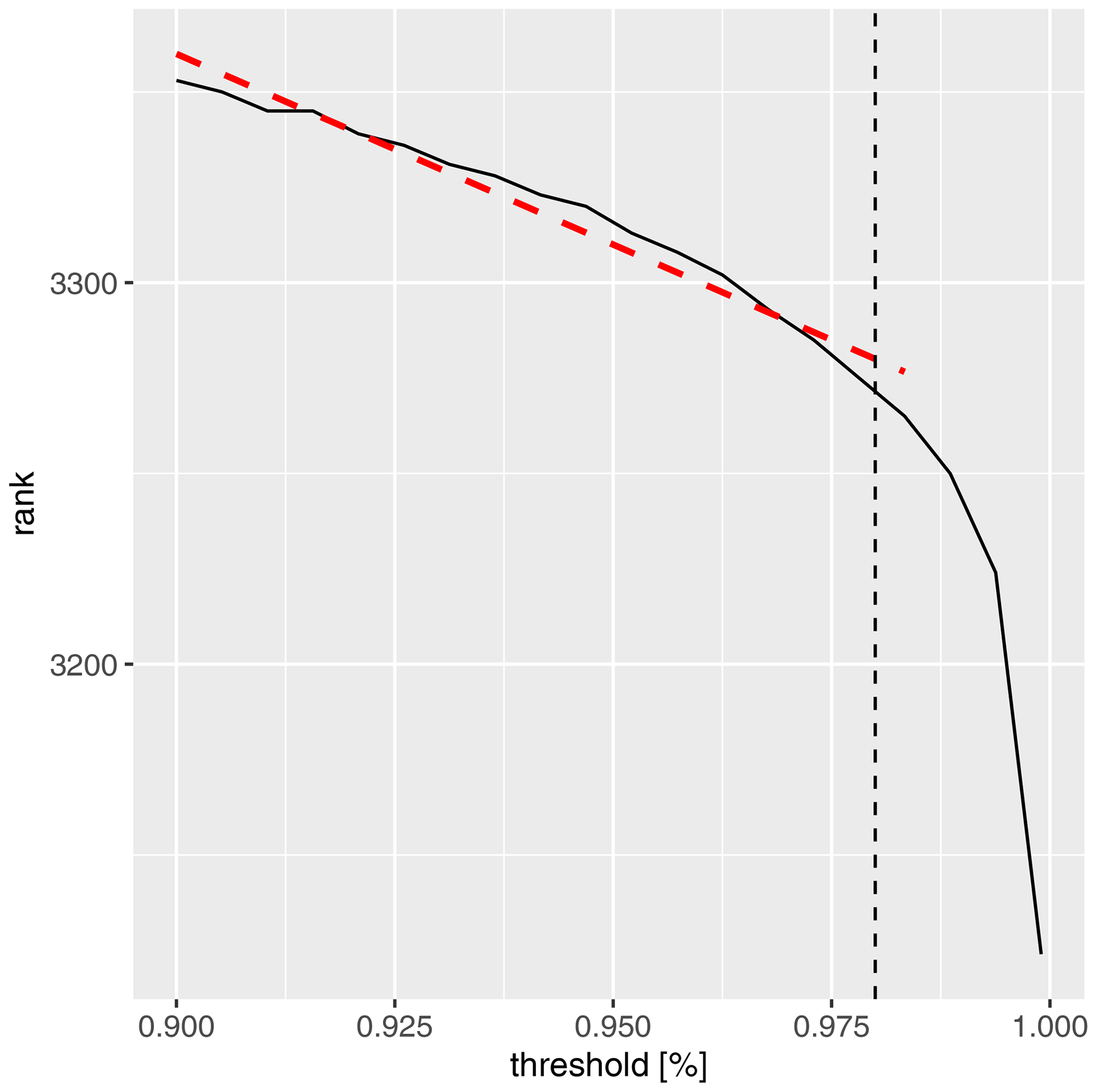
Figure 1 Rank of the TPDM, calculated for maxT2m and varying thresholds r₀ (Eq. 5). Vertical line: 98 % quantile. Red line: linear least-squares fit of the rank using a threshold between 90 % and 98 % quantile.

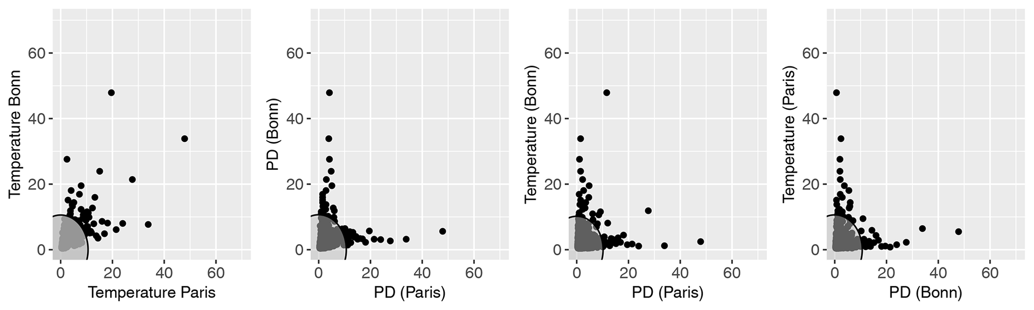
Figure 2 Scatter plots of Fréchet-transformed maxT2m and PD (black dots) at two grid points in COSMO-REA6 at Paris and Bonn. PD has been calculated from 15 d accumulated precipitation. The circle indicates the respective 98 % quantile, and the values inside the circle (gray shading) are not used for the estimation of the (cross-)TPDM.

Figure 2 shows maxT2m and the 15d PD at two grid points in COSMO-REA6 near Paris and Bonn. Only the data outside the gray shaded area (i.e., above the 98 % quantile) are used to estimate the cross-TPDM. The dependence between maxT2m at grid points with a distance between Paris and Bonn is strong even for the extreme values since the temperature variations are usually dominated by large-scale patterns and therefore still show dependencies, even at large distances. In contrast, the dependencies in the PD and between PD and maxT2m are much lower, which is due to the small-scale structures of the extreme values in the PD.

Figure 2 may be used to illustrate the asymptotic dependence/independence between Fréchet-distributed time series. The measure H(ω) of the angular component ω describes the tail dependence on the unit sphere ${\mathbb{S}}_{+}^{p-\mathrm{1}}$ (Sect. 2). With asymptotic independence, we expect the mass of H(ω) to be at the edges, so we do not expect an extreme event to occur in both variables simultaneously. With asymptotic dependence, corresponding probability mass exists on the unit circle, and we observe events that are extreme in both components.

As Jiang et al. (2020) point out, the assumption of asymptotic dependence, which is the basis of the concept of regular variations, may not be fulfilled. Jiang et al. (2020) focus on precipitation data, which are clearly not asymptotically dependent at the continental scale. This is less clear for regional-scale maxT2m and PD and cross-dependence. The TPDM method is nevertheless well suited to decompose (cross-)dependencies in our case since we typically do not reach the asymptotic limit for real data. For real data, we are more likely to be in the pre-asymptotic limit, which is characterized by significant dependencies, as seen in Fig. 2.

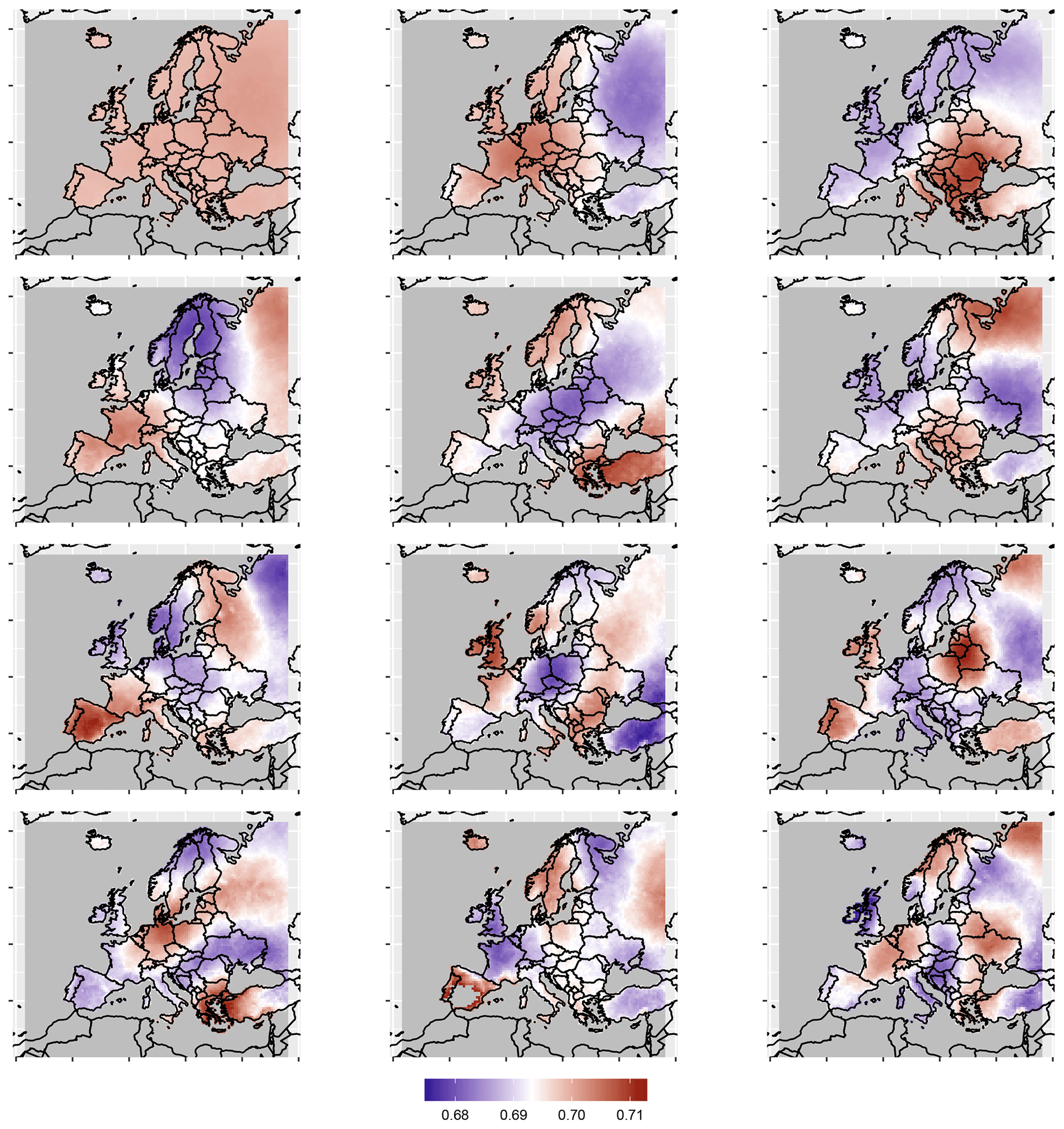
Figure 3 First 12 (from top to bottom, left to right) EVs of the TPDM for maxT2m in northern hemispheric summer months (JJA). Each vector is transformed to the positive real numbers ${\mathbb{R}}^p\to {\mathbb{R}}_{+}^p$ such that τ(0)=log(2) corresponds to zero.

7 Results

7.1 Spatial patterns of extreme daily maximum 2m temperature

We start our analysis with the estimation of the TPDM for maxT2m. The estimation is based on maxT2m values exceeding the local 98 % quantile on the reduced grid (see Sect. 6.1). Figure 3 shows the first 12 EVs of the TPDM. The first mode represents the nonzero spatial mean and consists of nearly constant values with only small variations of order 10⁻². Since the data are defined in ℝ₊ (see Sect. 2.3), the mean value is not removed unlike in standard PCA (cf.  Jiang et al., 2020; Cooley and Thibaud, 2019).

Higher-order EVs show large-scale patterns associated with the typical dipole and multipole structures also known from PCA. Since the EVs are transformed on ℝ₊, values >log (2) refer to positive and values <log (2) to negative anomalies (see Sect. 2.3). The wave-like structures are strongly reminiscent of westward-propagating Rossby waves, which are the main driving force for large-scale circulation patterns in northern mid-latitudes (see, e.g.,  Liu et al., 2020; Schubert et al., 2011; Gershunov and Douville, 2009).

An important question is how representative the EVs are and at what number of modes significant information is no longer added by further modes but overfitting prevails. In Figs. 4 and 5 we show explained variance and Q² as introduced in Sect. 4. The first EV contributes to about 25 % of the total variance, followed by less than 8 % for the second EV. As in Jiang et al. (2020) and Cooley and Thibaud (2019), the first EV (i.e. changes in the spatial mean maxT2m) dominates the variance. About 52 % (75 %) of the variance is explained by the first 10 (50) EVs. The out-of-sample information gain as measured by $Q_m^{\mathrm{2}}$ is positive for the leading 10 EVs. Both measures indicate that the first 10 EVs provide a representative subset for the spatial variation patterns of extreme maxT2m.

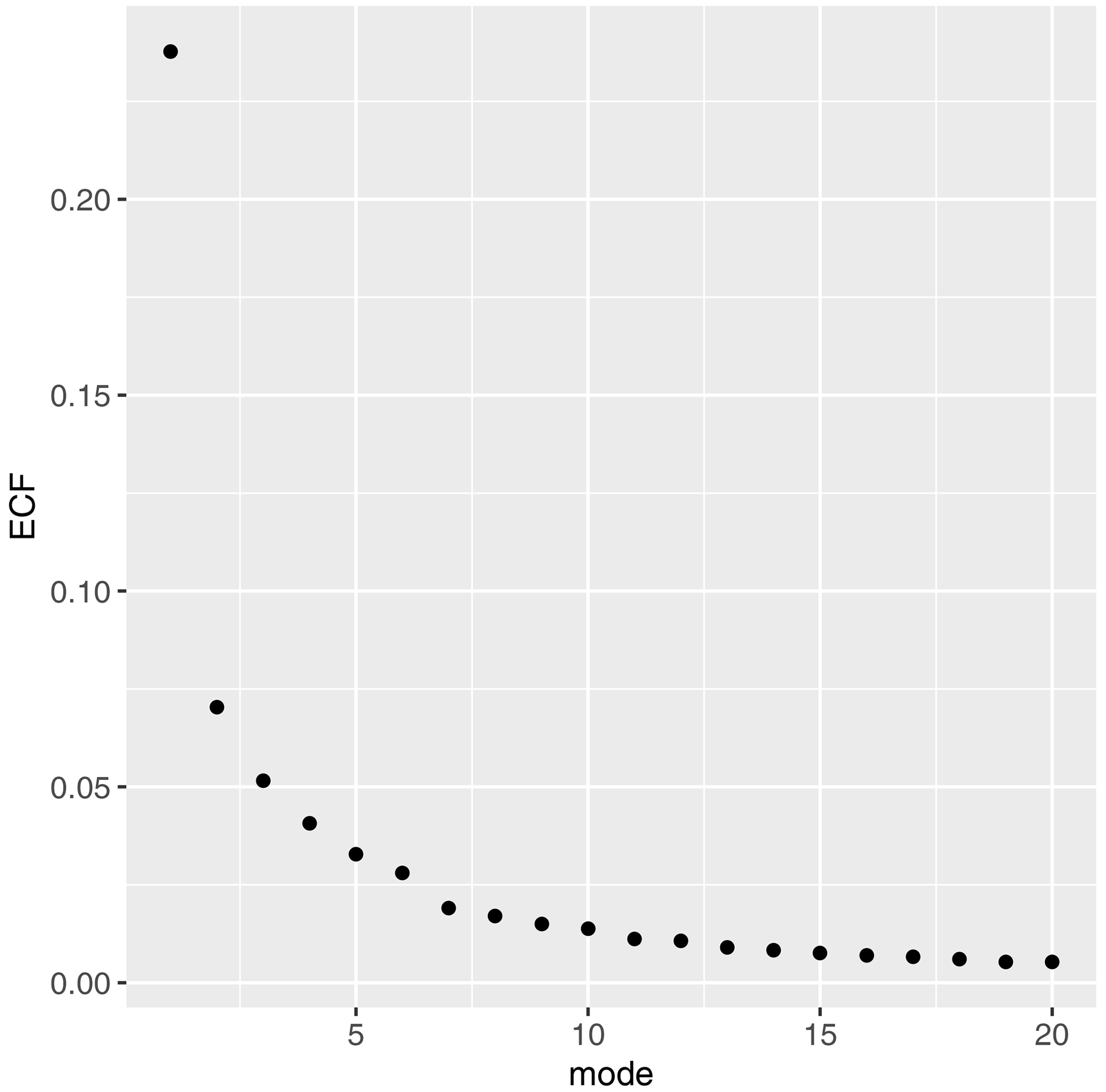
Figure 4 Explained variance ECF_k for each mode k (Eq. 16). Calculated from TPDM using maxT2m in northern hemispheric summer months (JJA).

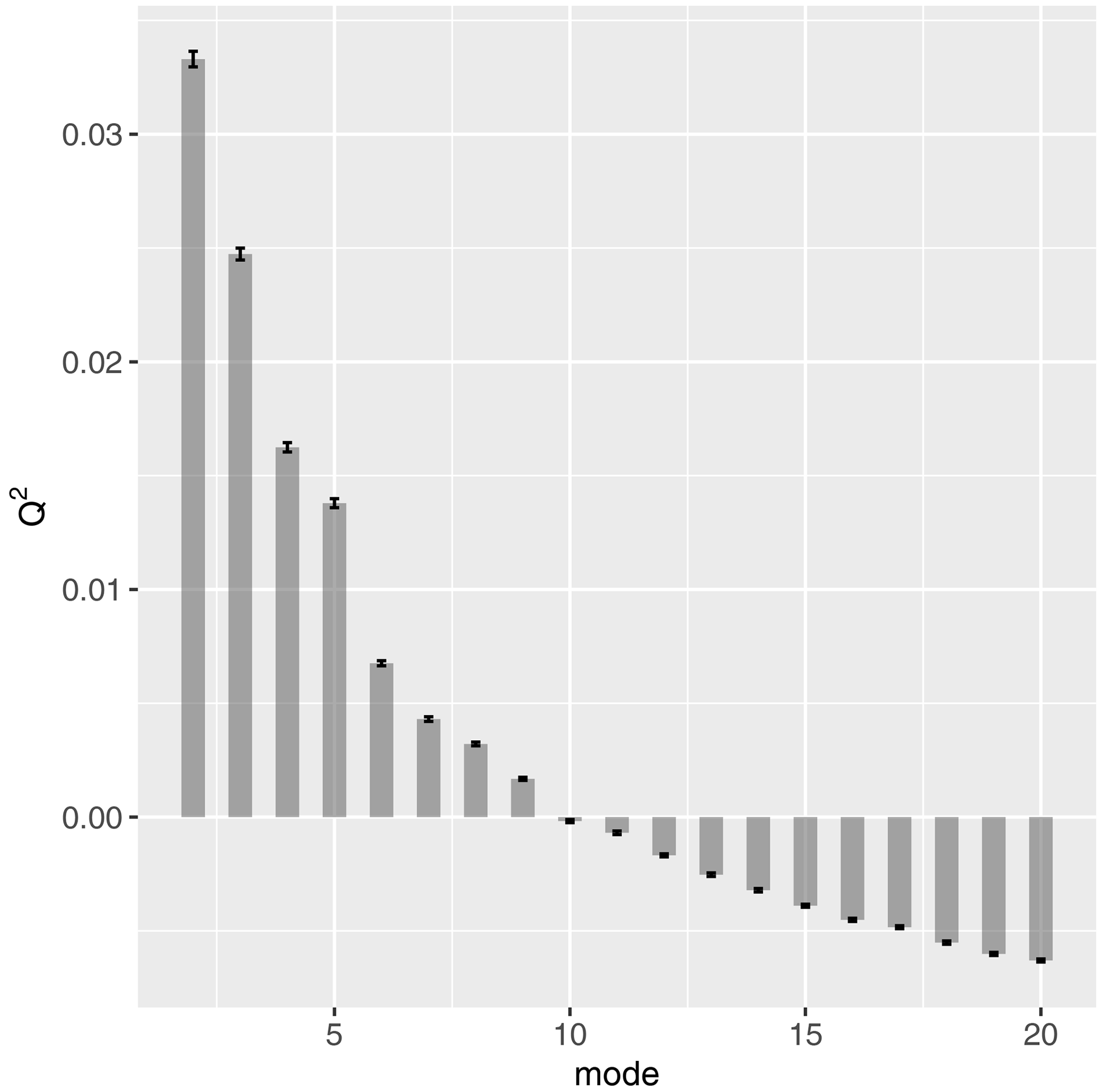
Figure 5 $Q_m^{\mathrm{2}}$ for the first m=20 modes (Eq. 17). Calculated from TPDM for maxT2m in northern hemispheric summer months (JJA). The error bars indicate the standard error determined using 100 bootstrap samples.

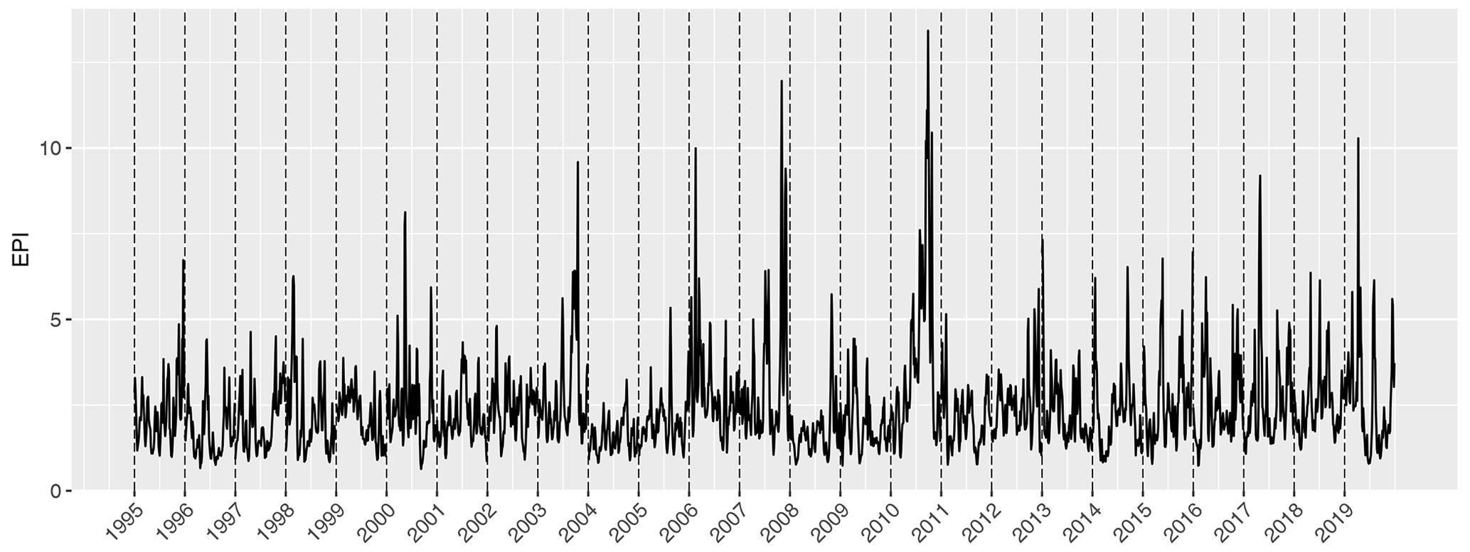
Figure 6 EPI^η as calculated from first 10 PCs after a PCA of the TPDM for maxT2m. Shown are the northern hemispheric summer months (JJA) from 1995 to 2019.

7.2 Extreme pattern index for temperature extremes

Our calculation of the EPI^η (Eq. 18) uses the first 10 PCs η_k with $k=\mathrm{1},\mathrm{\dots },\mathrm{10}$. The time series of the PCs for the first six EVs are displayed in Fig. A1 in the Appendix. Figure 6 shows EPI^η for the June to September months from 1995 to 2019 with values varying between 0.5 and 13.5. Peaks in EPI^η indicate intense heat waves within the studied region. Although the 2010 summer heat wave prominently stands out in EPI^η, we also identify other peaks associated with typical heat waves. The large outliers in the PCs as well as in EPI^η indicate a heavy tail behavior, as already shown by Cooley and Thibaud (2019) for the PCs.

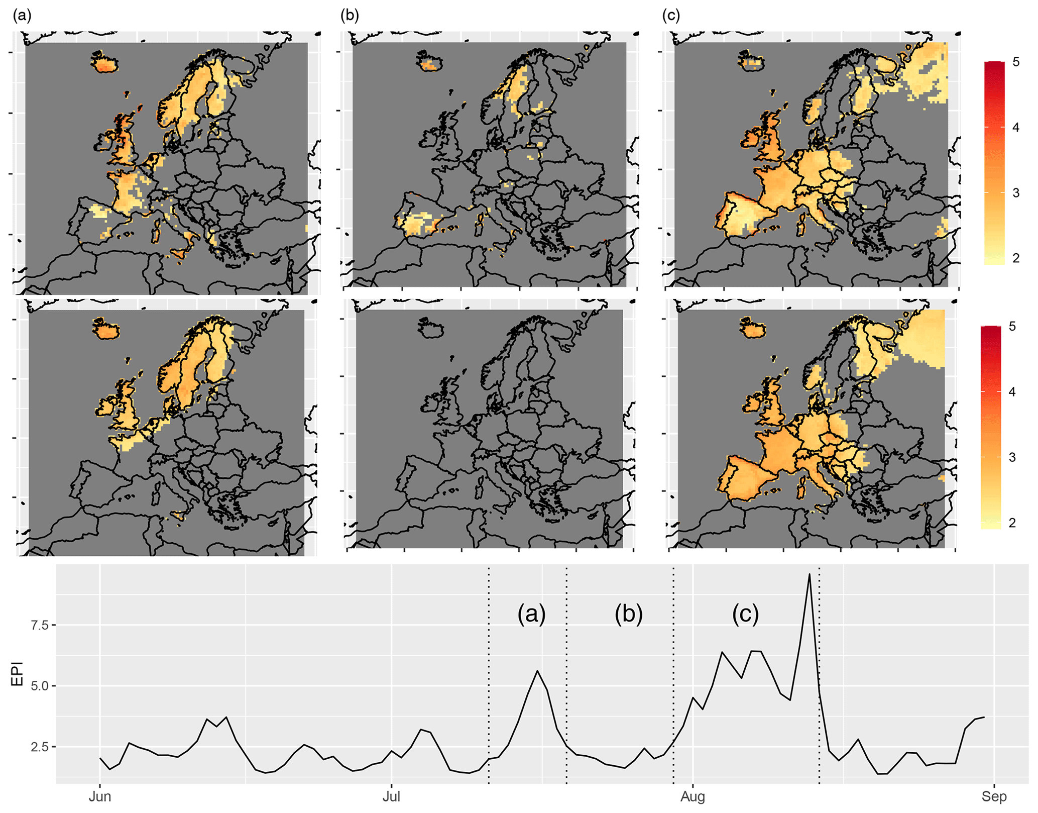
Figure 7 Overview of the temporal evolution of the 2003 heat wave. Top: pattern of mean anomalies within the periods (a) 11–19 July 2003, (b) 19–30 July 2003, and (c) 30 July–14 August 2003. We show the maxT2m anomalies (upper pattern) and the reconstruction, using the first 10 modes of PCs (lower pattern). All patterns use the same color scale and only show values exceeding the 98 % quantile, respectively. Bottom: EPI^η as in Fig. 6 but for JJA months in 2003.

We will now examine the two heat waves of 2003 and 2010 in more detail using our framework. Both heat waves have been extensively studied and analyzed in the existing literature. The 2010 heat wave is characterized by the highest peak EPI in the period considered. This indicates that the 2010 heat wave was the most extreme event in terms of its combination of intensity and spatial extent over the period considered. The 2003 heat wave, on the other hand, did not reach the highest peak but is characterized by its long, highly pronounced duration. Finally, both heat waves had significant impacts on socio-economic systems, underlining their importance for understanding extreme heat events (see Beniston, 2004; Barriopedro et al., 2011; Kueh and Lin, 2020; Schubert et al., 2011; Gershunov and Douville, 2009). Figure 7 (bottom panel) shows EPI^η for the June to September months in 2003. The respective averaged maxT2m anomalies are shown in the upper panels for the periods during periods as marked with (a) to (c). We observe a first heat wave in mid-July (a) in western Europe, which is most pronounced over the United Kingdom, Iceland, and Norway. This short-term event is followed by a few non-extreme days (b), after which we observe a very severe heat wave over central and southern Europe from late July to mid-August (c) (see also  García-Herrera et al., 2010; Liu et al., 2020). In Fig. 7 we also display the reconstruction of the maxT2m fields using only the leading 10 EVs. The spatial structure of the heat wave pattern in maxT2m is well represented within the 10-dimensional subspace. The reconstructed patterns are somewhat smoother and thus more clearly highlight the areas affected by the heat wave. Thus, the subspace spanned by the 10 eigenvectors of the TPDM is sufficient to describe the 2003 heat wave and fulfills the goal of a compact description of large-scale heat waves.

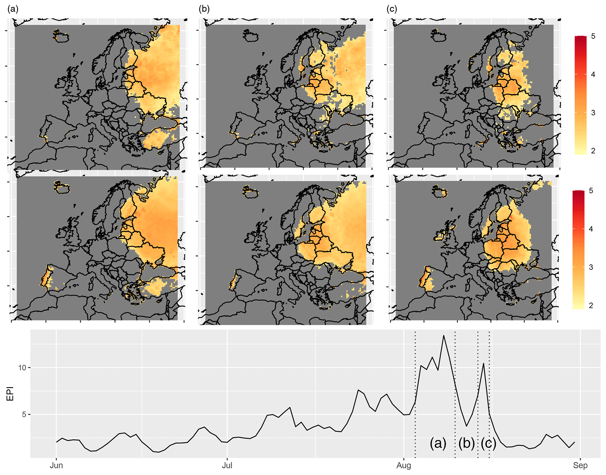
Figure 8 Overview of the temporal evolution of the 2010 heat wave. Top: pattern of mean anomalies within the periods (a) 3–10 August 2010, (b) 10–14 August 2010, and (c) 14–16 August 2010. We show the maxT2m anomalies (upper pattern) and the reconstruction, using the first 10 modes of PCs (lower pattern). All patterns use the same color scale and only show values exceeding the 98 % quantile, respectively. Bottom: EPI^η as in Fig. 6 but for JJA months in 2010.

In Fig. 8, we analyze the Russian heat wave in 2010. High values of EPI^η consistently capture their evolution from the second week of July to mid-August, as analyzed, e.g., in Barriopedro et al. (2011) or Liu et al. (2020). Since we observe the strongest expressions of EPI^η in the first half of August, we focus on this period in the following. The beginning of August is characterized by the most intensive phase of the heat wave according to EPI^η (a), with its center located over Moscow, western Russia. In the second week, we observe a westward shift of the maxT2m anomalies, accompanied by a short drop in EPI^η (b). Then the heat wave intensifies again for 2 d, with a new center over Belarus and Lithuania (c), before it collapses in mid-August. This particular feature of the 2010 heat wave has received little attention in the literature, although it is clearly visible in station measurements in, e.g., Moscow (Grumm, 2011). Consequentially, the Russian heat wave can also be well described by our method.

Table 1 Periods of strongest heat waves defined by EPI and GRD events. Periods indicated in black are within the top 15 strongest events using the respective index (EPImean, GRDsize, and GRDmean). Periods in bold are heat waves with a lower rank than 15, and underlined periods show no correspondence in the respective counterpart (EPI or GRD).

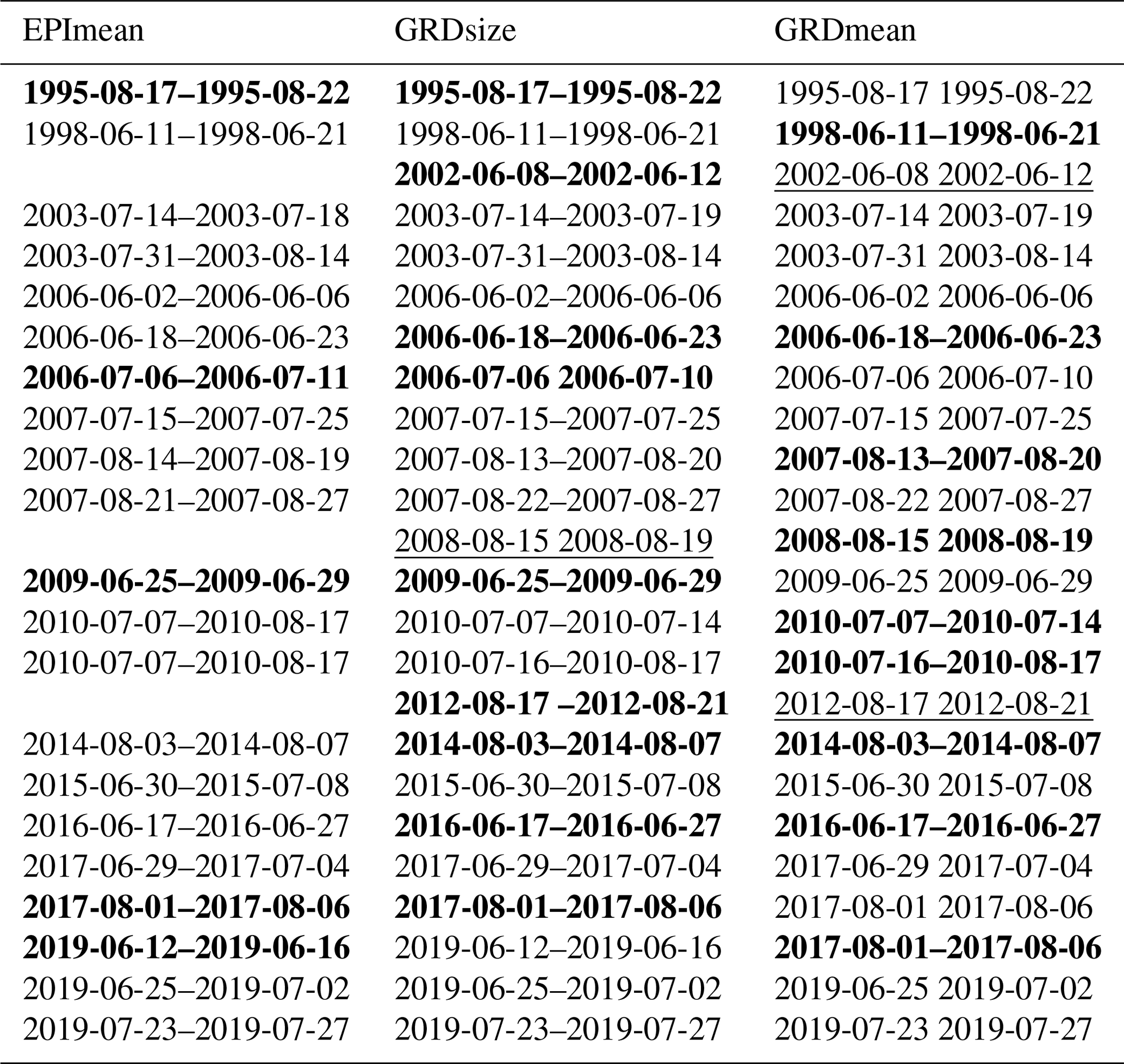
To further evaluate the suitability of EPI^η for heat wave detection and representation, we compare event definitions using EPI^η with other heat wave definitions. A heat wave is usually defined on the basis of grid points (hereafter GRD event), e.g., a 5 d continuous exceedance of the 98 % quantile of maxT2m, with seasonal trends removed. A GRD event exists when a 5 d continuous exceedance occurs in at least 3 % of the grid points. Using maxT2m of COSMO-REA6, we obtain a number of 32 GRD events during the summer months in 1995–2019 in Europe. To rank heat wave events in terms of their “extremeness”, DWD compares predefined heat waves (i.e. GRD events) based on the properties of duration, maximum number of grid points affected (GRDsize), and average magnitude of maxT2m anomalies (GRDmean)³. The time period of the 15 strongest GRD events with respect to GRDsize and GRDmean is displayed in black in Table 1.

We define an EPI event as a period when EPI^η exceeds the 80 % quantile for at least 5 consecutive days. The threshold is chosen so that we get a similar number of heat waves for the EPI events as for the GRD events, yielding a total of 28 heat waves. In Table 1, we compare the top 15 EPI events according to their average EPI^η (EPImean), with the top 15 GRD events according to their GRDsize and GRDmean. Of the top 15 GRD events, 3 (June 2002, August 2008, and August 2012) are not classified as EPI events. For each of these events, the maxT2m fields exceeding the 98 % quantile and the EPI^η are shown in the Appendix Fig. A2. We find EPI^η exceeds the 80 % quantile in all three GRD events, but the duration is less than 5 d in each case. Of the top 15 EPI events, 13 are identified as being among the top 15 GRD events in terms of GRDsize as well, suggesting that EPI^η is particularly successful in the identification of large-scale extremes. This is largely due to the property of PCA, which detects large-scale patterns mainly in the first few modes. Large-scale extremes are thus weighted more strongly than small-scale events.

The Cooley and Thibaud framework requires the assumption of independent and identically distributed samples. This assumption is generally not given for daily values of maxT2m and PD. However, it turns out that our method is quite robust in this respect. We evaluate this in Appendix Fig. A3 using the EPI calculated on the one hand from the patterns of daily maxT2m data and on the other hand from the patterns of weekly maxima of maxT2m. It can be seen that the EPI is robust to small deviations in individual patterns. The range of EPI values changes slightly as the first 10 modes explain a higher proportion of the variance.

7.3 Decomposition of the cross-TPDM for maxT2m and PD

We have shown that the decomposition of the TPDM provides a set of spatial patterns to describe extremal dependencies in maxT2m and leads to a suitable definition of a heat wave index. We now turn to the cross-TPDM, which encodes the extremal covariability of maxT2m and PD. Commonly used indices, e.g., the standard precipitation index (SPI), are calculated on relatively long accumulation times from 3 to 48 months (McKee et al., 1993). However, so-called “flash droughts”, e.g., occur instantaneously at sub-seasonal scales. They are characterized by rapid development and intensification of drought, usually accompanied by exceptionally high temperatures (see, e.g., Peters et al., 2002; Hunt et al., 2009; Cook et al., 2018). To capture this structure, Mo and Lettenmaier (2016), e.g., calculate PD using 5 d precipitation averages. Here, we want to capture both perspectives on the dynamics and the evolution of compound heat wave and drought events and therefore assess extremal covariability for different accumulation times from 11 to 47 d.

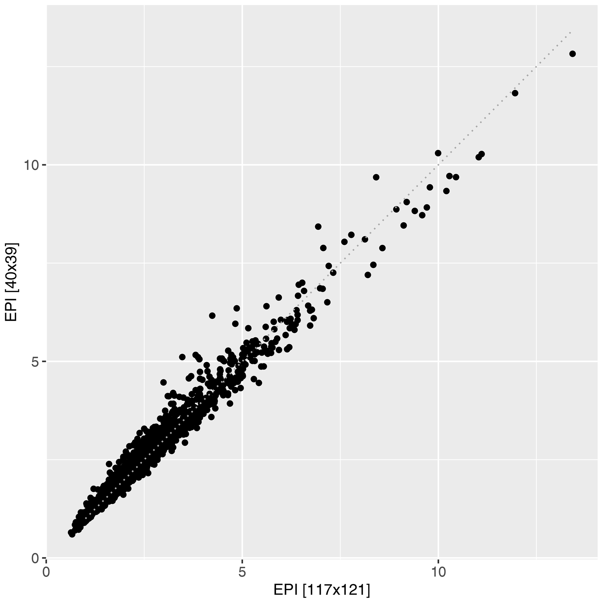
To allow for a computation of the cross-TPDM for many different accumulations times, we need to lower the computational costs by further reducing the grid size. For this purpose, we increase the neighborhood in the COSMO-REA6 grid to 21×21 grid points and take the respective maximum of PD and maxT2m as the value (in Sect. 7.2 we used a neighborhood of 7×7 grid points). With this approach, we obtain a grid of size 40×39. To ensure that no important information gets lost in this new reduction, in Appendix Fig. A4 we exemplarily show the EPI^η as calculated in Sect. 7.2 against the EPI^η on the highly reduced grid. The differences in the temporal behavior are small, and the EPI^η is robust to this further data reduction. Although not shown here, we have produced similar diagrams for the other indices we have defined, with similar results.

Not only the duration of a dry spell but also when it occurs in relation to the heat wave can be important for dynamic interpretation. For example, there is evidence that a dry phase can promote the development of an intense heat period (see, e.g., Sousa et al., 2020). To account for different feedback mechanisms between PD and maxT2m, we introduce a time shift between PD and maxT2m, in the sense that PD leads maxT2m in time when there is a negative shift. The cross-TPDM and its decomposition using SVD are calculated for each time shift and accumulation time, respectively.

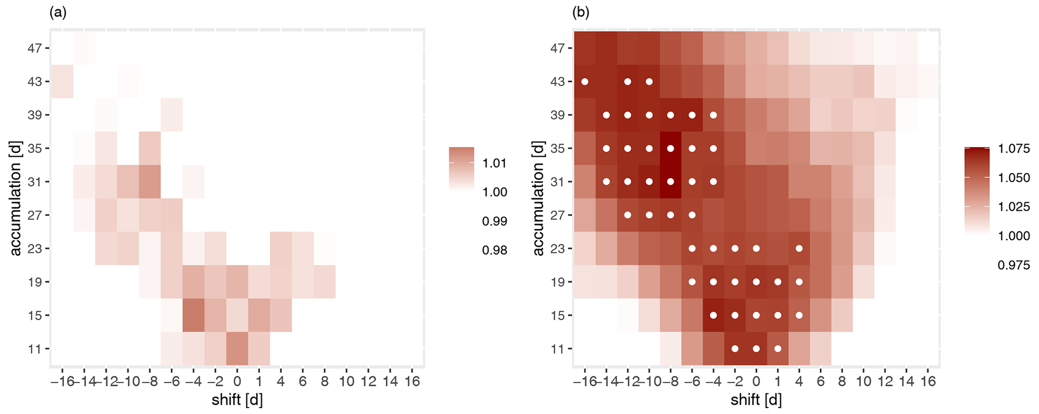
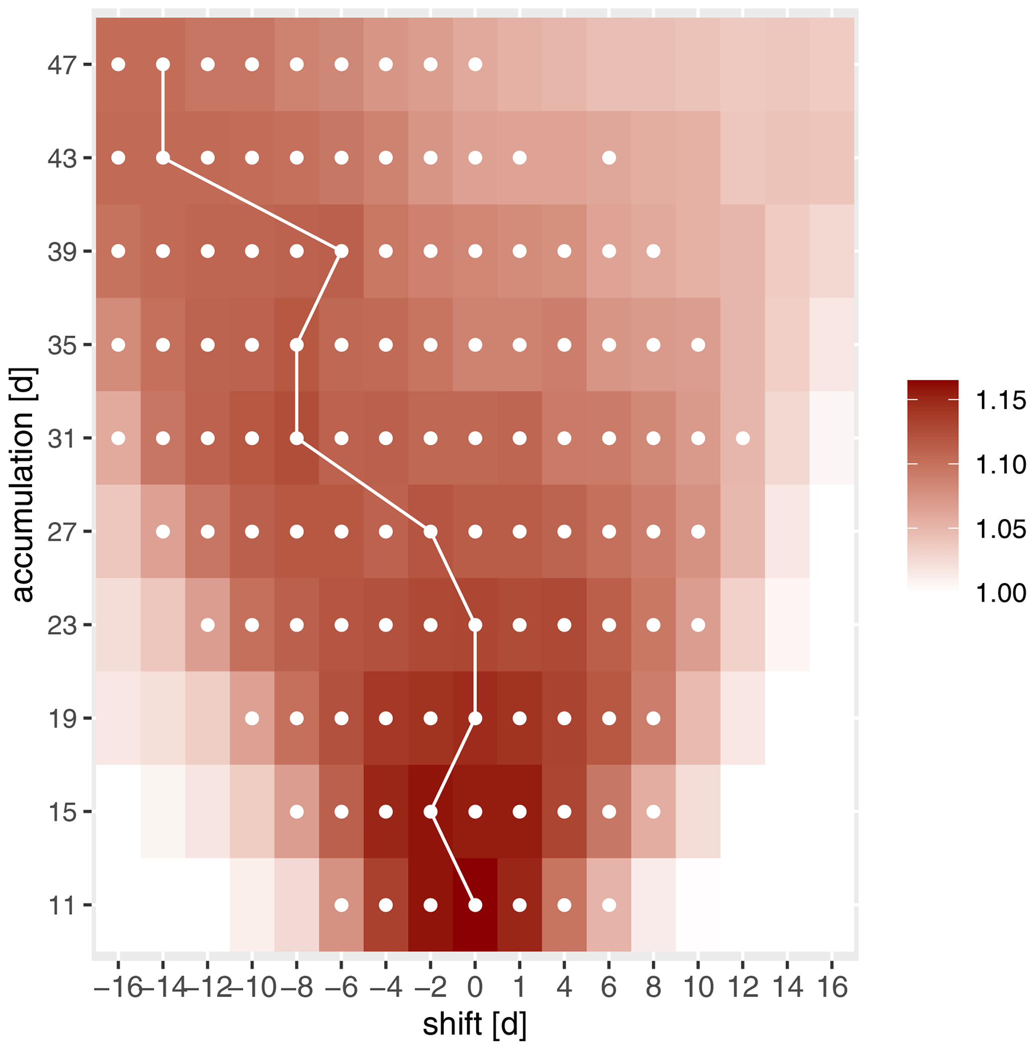
Figure 9 First and first + second singular values of the cross-TPDM calculated from maxT2m and PD in northern hemispheric summer months for varying shift and accumulation times. Each value has been normalized by the respective mean of 100 bootstrap samples where the temporal relation is destroyed. White dots indicate values exceeding the 95 % confidence interval of “no statistical relation”.

We assess statistical significance based on the singular values. To this end, we generate a 100-head bootstrap sample where we draw maxT2m and PD of a season independently so that the temporal relationship is destroyed while seasonality is preserved in the data. In Fig. 9, we show the first and the sum of the first and second singular values of the cross-TPDM, normalized by the respective average over the bootstrap samples. This is shown as a function of time shift and accumulation level. For values >1 the measure of the extremal covariability between maxT2m and PD is larger than on average in the bootstrap sample. White dots indicate values that exceeded the 95 % confidence interval of the values in the bootstrap sample with “no statistical association”.

For short accumulation times, maximum association is obtained for instantaneous anomalies. For higher accumulation times, the association is maximal for negative shifts when anomalies in PD precede the maxT2m anomalies. This indicates that a heat wave is preferentially formed when it is preceded by a drought period. Considering the sum of more singular values (see Appendix Fig. A5 for the first 10 singular values), this time-shifted dependence structure weakens but remains significant. We conclude that the statistical association between the large-scale patterns in matT2m and PD is significant and that the accumulation time of PD must be evaluated together with a temporal shift.

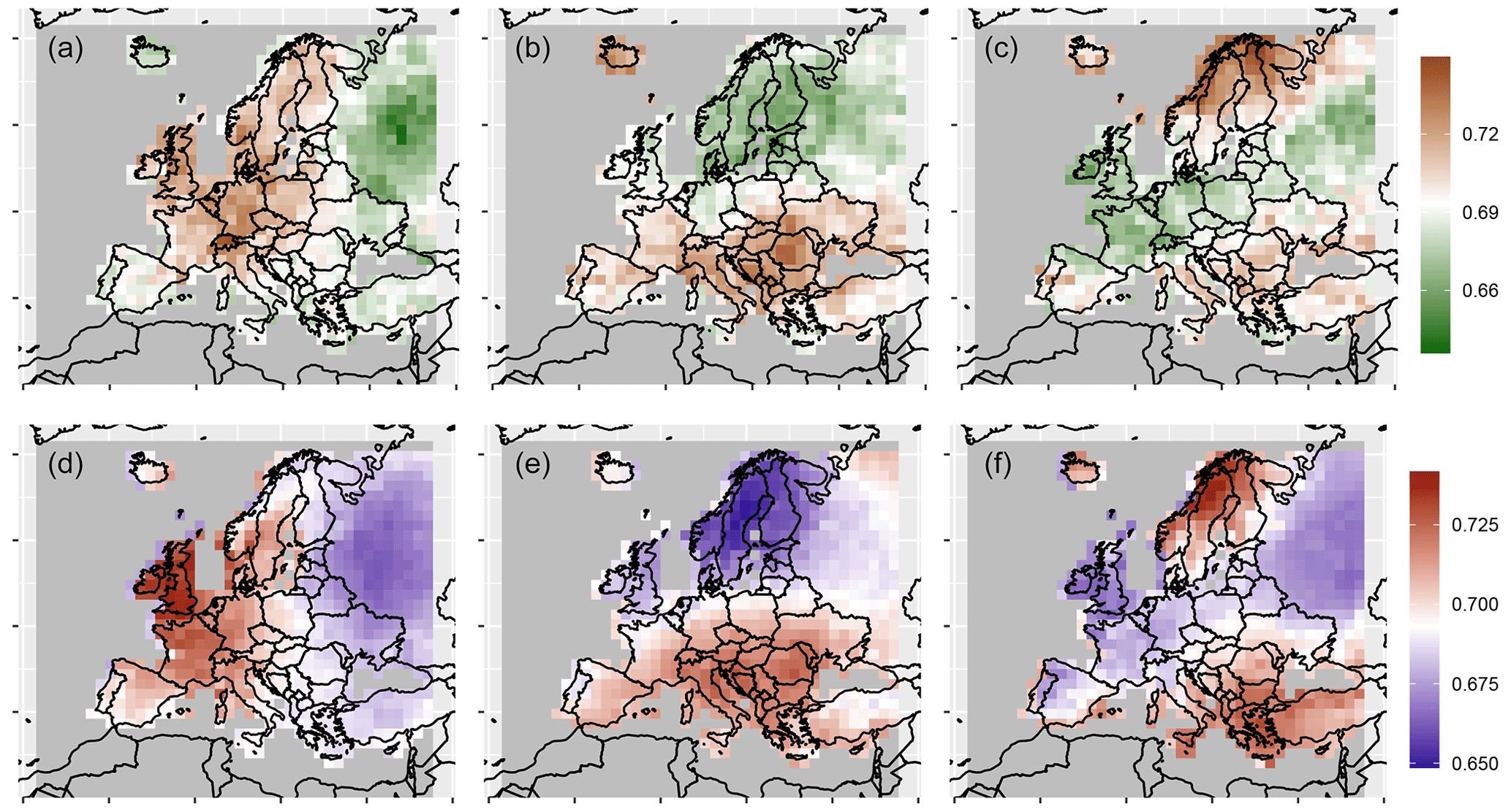
Figure 10 Second, third, and fourth left and right SVs of the cross-TPDM, associated with anomalies in maxT2m (d, e, f) and 11 d PD (a, b, c). As in Fig. 3, we transformed each vector to the positive real numbers ${\mathbb{R}}^p\to {\mathbb{R}}_{+}^p$ such that τ(0)=log (2) corresponds to zero.

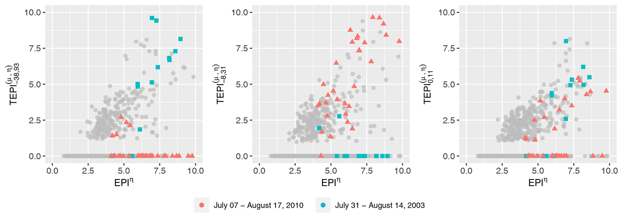
Figure 11 Scatter plot of EPI^η and TEPI^μ,η. TEPI^μ,η is shown for calculation from PD using three different combinations of shift and accumulation (11 d accumulation, 0 d shift; 35 d accumulations, 8 d shift; and 93 d accumulation, 46 d shift). All indices were calculated using the first 10 PCs of the cross-TPDM from maxT2m and PD for northern hemispheric summer months. The 2010 and 2003 heat waves (31 July–14 August 2003; 7 July–17 August 2010), as identified in Table 1, are highlighted in blue and red, respectively.

We now turn to the large-scale patterns of extremes in maxT2m and PD. In Fig. 10, we show the patterns for an accumulation time of 11 d and a time shift of 0 d. The large-scale patterns again show the characteristic wave-like structure previously discussed in Sect. 7.1. The corresponding anomalies in maxT2m and PD have a very similar structure, with the regions of the strongest gradients in PD slightly shifted compared to the gradients in maxT2m (second pattern – eastwards, third pattern – southwards). Although a physical interpretation of the SVs should always be approached with caution (see Sect. 3.3), it is possible that eastward-propagating Rossby waves (Sect. 7.1) could explain this pattern if, for example, strong gradients in the temperature fields are associated with frontal systems typically associated with precipitation. The leading patterns are also very similar for other accumulation times and time shifts.

7.4 Extremal pattern indices for compound maxT2m and PD extremes

As in Sect. 5 we base our calculation of an extremal pattern index on the expansion coefficients, where η_k represents the respective expansion coefficient of maxT2m and ν_k of PD. We calculate the EPI^η,ν (Eq. 19) and the TEPI^η,ν (Eq. 20) using η_k and ν_k of the leading 10 SVD modes of maxT2m and PC, respectively. As a threshold for the TEPI^η,ν, we use the 90 % quantile, respectively. This gives us a sufficient number of events without losing focus on the extremes. In this way, we obtain a flexible tool for the analysis of different event characteristics of compound extremes in maxT2m and PD.

Our investigation focuses on three cases with varying accumulation periods and lead times for PD anomalies: one with 11 d accumulations and immediate anomalies, another with 35 d accumulations and a PD anomaly lead time of 8 d, and a third case with 93 d accumulations and a PD anomaly lead time of 38 d. The first case represents short-term, coincident events, while the second and third cases represent monthly and seasonal PD driving a heat wave. In all cases, we find significant statistical dependence between maxT2m and PD (Fig. A5). Although not shown, we obtain a significant value of 1.13 for the third case 93 d accumulation and 38 d shift. Figure 11 displays the TEPI^η,ν for all cases. The heat waves in 2003 and 2010 are indicated with colors.

Both the 2003 and 2010 heat waves show a strong signal in instantaneous TEPI. TEPI^η,ν events coincide with heat wave events as indicated by the EPI^η, suggesting that both heat waves were accompanied by short-term PD. This indicates typical weather conditions during heat waves with clear skies, strong solar radiation, and little to no precipitation (Fischer et al., 2007).

Furthermore, the 2003 heat wave was preceded by a PD that was mainly evident on a seasonal timescale, whereas the 2010 heat wave was preceded by a more pronounced PD on a monthly timescale. In both cases, the high agreement of TEPI^η,ν and EPI^η suggests that PD contributed to the extreme maxT2m during 2003 and 2010 (see also  Fischer et al., 2007; Fink et al., 2004; Zaitchik et al., 2006; Christian et al., 2020).

Thus, the heat waves in 2003 and 2010 display different dynamics concerning common extremes of PD and maxT2m. Our TEPI definition effectively captures these characteristics, demonstrating that both events meet the IPCC definition of compound events as “two or more extreme events occurring simultaneously or sequentially” (Seneviratne et al., 2012).

We thus demonstrate that our definition of TEPI for different accumulation times and temporal shifts summarizes many characteristics of compound extremes and represents a suitable index.

8 Discussion and conclusion

In this study, we apply the promising approach of Cooley and Thibaud (2019) to describe extremal dependencies using the TPDM. The TPDM has comparable properties to the covariance matrix and can be decomposed similar to PCA while focusing on the tail behavior of the variables. To describe the dynamics of large-scale temperature extremes, we calculated the TPDM based on maxT2m and identified typical temperature patterns of European heat waves. Our results are in line with previous studies that identify large-scale blocking events as the primary mechanism behind European heat waves (e.g. Schubert et al., 2014; Stefanon et al., 2012). We determine the optimal number of patterns to describe the main features of European heat waves and show exemplarily for the 2003 and 2010 heat waves that the description of the dynamics of large-scale temperature extremes is suitable with only the 10 leading eigenmodes.

We define the extremal pattern index (EPI) based on the time series of PCs and obtain a pattern-based spatial aggregation index. Thus, we can specifically identify spatially related extreme events with minimal reliance on pre-defined thresholds and regions of influence in grid point space. Although we cannot completely eliminate the use of a threshold, as it is a fundamental factor in estimating extreme dependencies based on the TPDM, all data, even those below the threshold, are included in the EPI estimator. We can show that this results in little information being lost with respect to the heat wave description.

Using the 2003 and 2010 European heat waves as examples, we examine how well the EPI captures the essential characteristics of heat waves. The temporal progression of both heat waves can be effectively illustrated using the EPI and aligns with the findings of previous analyses. Some characteristics, such as the collapse of the 2010 heat wave between 10 and 14 August, can be clearly identified using the EPI yet have received little exploration in the existing literature. An additional condition of heat waves besides spatial extent and intensity is usually temporal persistence. This condition can also be applied to EPI by defining heat waves. In Sect. 7, e.g., we define a heat wave (i.e., an EPI event) such that the EPI exceeds a threshold for at least 5 consecutive days. We propose an EPI-based definition of heat waves that, compared to a conventional definition, gives very consistent results. This shows that the EPI is suitable as an alternative to conventional heat wave indices with minimum reliance on user-defined thresholds. The EPI is thus a powerful tool for, e.g., attribution studies, climate monitoring, and characterization of extreme weather conditions.

Since pronounced heat waves over Europe cover a large part of the area studied, the spatial mean describes the course of the heat waves relatively well. Nevertheless, the higher modes of the PCs contribute significantly to the description of heat waves, as we discuss in Sect. 7.1. It can be assumed that the dominant influence of the first PC on the EPI would decrease when analyzing a larger geographical area.

To include the temporal persistence of heat waves as another condition, one could include only those patterns that exhibit a certain persistence and then aggregate them over time. However, too hard a condition could be detrimental.

After initially focusing on the description of heat waves using maxT2m, we extend our approach and go beyond the examination of individual variables. We deal with common extremes in maxT2m and PD. To this end, we propose a cross-TPDM model as an analog to the cross-covariance matrix that describes pairwise extremal dependencies between the two variables. Previous studies for compound events have usually referred to monthly or even seasonal variables (Wu et al., 2019; Hao et al., 2019). We calculate PD from daily precipitation using different duration scales. To generalize our approach and apply it to compound events as well, we shift the time series against each other. This allows us to investigate the dynamics of compound extremes in maxT2m and PD, even at relatively short duration levels. Using the singular values following an SVD, we analyze the dynamics of compound extremes in PD and maxT2m and show that preceding extremes in PD exert a significant influence on the evolution of heat waves (see, e.g.,  Christian et al., 2020). The investigation of additional variables such as hydrological drought indices and boundary layer heights would undoubtedly be interesting and may provide new insights into physical relationships.

Last but not least, we extend the EPI from considering a single variable to describing simultaneous extremes in two variables. We introduce a threshold-based estimator, the TEPI, which ensures simultaneous extremes of the underlying patterns. To demonstrate the utility of the TEPI, we again focus on the 2003 and 2010 heat waves and analyze their different dynamics in terms of compound extremes in maxT2m and PD using the TEPI. We analyze both heat waves using two event types: short-term coincident events and long-term precipitation deficit triggering a heat wave. In both cases, we can use TEPI to reconstruct the known characteristics of these events and demonstrate its effectiveness as a valuable tool for analyzing compound extremes. TEPI is a way to focus on specific events. A disadvantage of our formulation of TEPI is the hard condition of exceeding a threshold (see Fig. 11). We need to investigate whether a less strict selection or weighting would be beneficial.

There are several indicators for assessing climate indices (see, e.g., Keyantash and Dracup, 2002; Redmond, 1991). Both EPI and TEPI are robust to application to different data sources, although we believe they are most successful in identifying large-scale extremes. In principle, they are applicable to point (e.g., measured data) and gridded data sets. The mathematical theory and derivation are quite complex, but the application is comparatively simple since existing functions for PCA and SVD, etc., can be used in various programming languages. Jiang et al. (2020) also make their R code for calculating TPDM, data pre-processing, and performing PCA available.

The cost-intensiveness of calculating TPDM based on high-resolution climate models is a universal problem that affects methods for dealing with spatial dependencies. This can possibly be solved by clever mathematical reformulation or extension of the working memory. As shown in Fig. A4, the data reduction approach we propose, using the spatial block maximum, provides a robust estimate of the EPI.

The TPDM assumes asymptotic dependence. However, we recognize that this assumption may not hold for maxT2m, PD, and their interdependencies. As Jiang et al. (2020), we nevertheless choose to decompose using the TPDM, as it opens up a new way to examine extreme patterns in maxT2m and PD. The resulting patterns are consistent with previous findings in the field and provide a meaningful dynamic context.

Appendix A

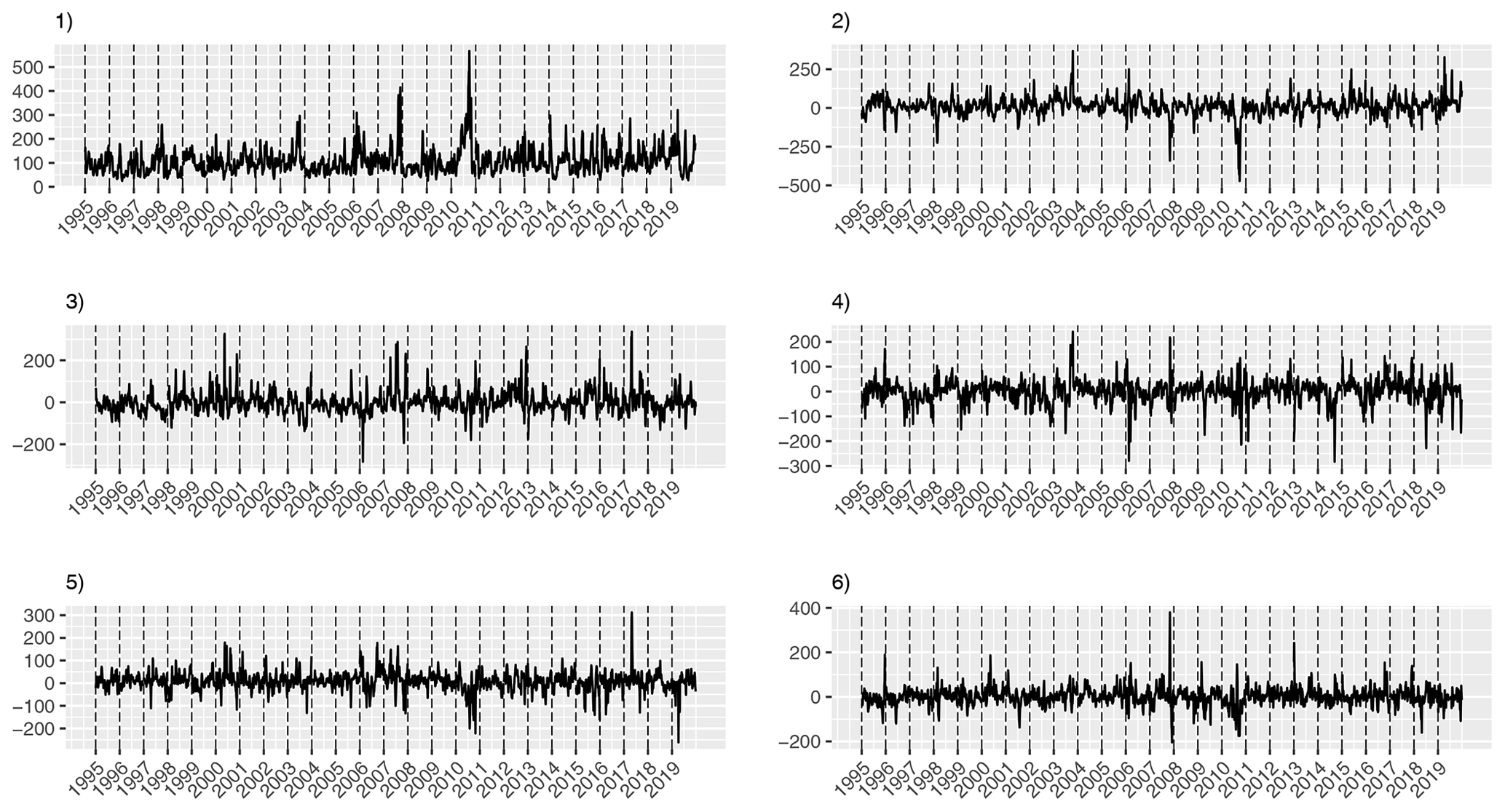
Figure A1 First six (from left to right, top to bottom) PCs of the TPDM as calculated from maxT2m in northern hemispheric summer months (JJA).

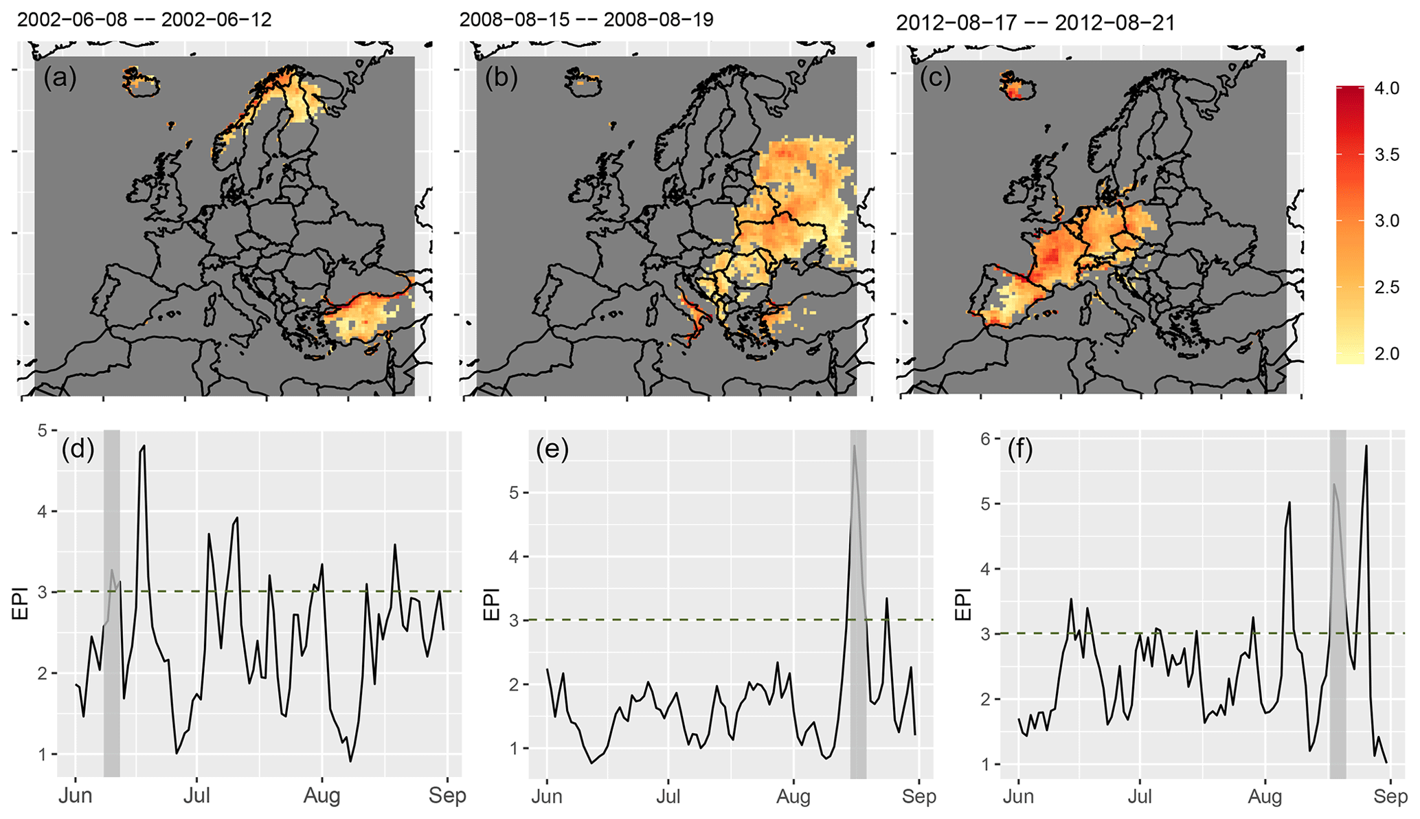
Figure A2 EPI^η and maximum maxT2m anomaly of top 15 EPI events (according to EPImean) which are not identified as GRD events (Sect. 7.2). (a, b, c) Maximum maxT2m anomaly. Shown are only grid points exceeding the 98 % quantile. (d, e, f) EPI^η as shown in Fig. 6 but for single years 2002, 2008, and 2012. Time periods of corresponding EPI events are marked in gray.

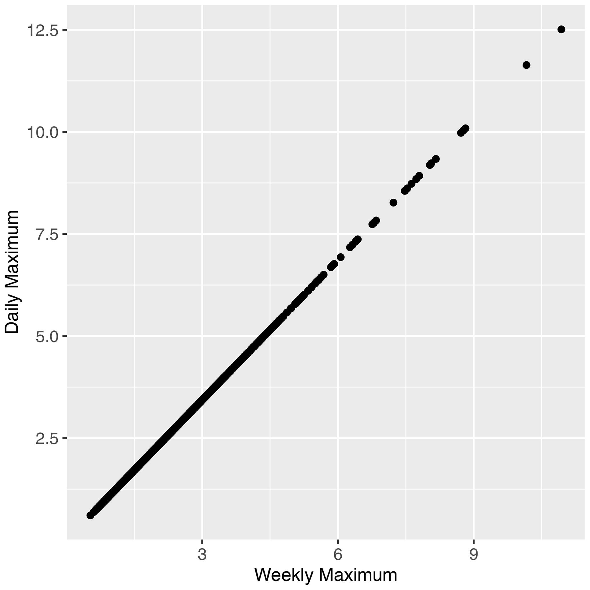
Figure A3 Scatter plot representation of EPI^η calculated on EVs and eigenvalues of daily maxT2m and weekly maximum of maxT2m.

Figure A4 Scatter plot representation of EPI^η calculated on [117×121] grid (see Sect. 7.2) vs. EPI^η calculated on [40×39] grid (Sect. 3).

Figure A5 As in Fig. 9 but for the sum of first 10 singular values. The white line connects the maximum values over each accumulation stage.