On inference of boxplot symbolic data: applications in climatology

This paper presents a pioneering study on the inference of boxplot-valued data using both Bayesian and frequentist approaches within a multivariate framework. This approach leverages complex yet intuitive representations to make large datasets more manageable and enhance their interpretability, which is invaluable in the age of big data. Boxplot-valued data are particularly important due to their ability to capture the inherent variability and distributional characteristics of complex datasets.

In our study, we propose novel methodologies for parameter estimation and density estimation for boxplot-valued data and apply these techniques to climatological data. Specifically, we utilize data from the Berkeley Earth Surface Temperature Study, which aggregates 1.6 billion temperature reports from 16 pre-existing archives affiliated with the Lawrence Berkeley National Laboratory. Our methods are validated through extensive simulations comparing the efficiency and accuracy of Bayesian and frequentist estimators.

We demonstrate the practical applicability of our approach by analyzing summer average temperatures across various European countries. The proposed techniques provide robust tools for analyzing complex data structures, offering valuable insights into climatic trends and variations. Our study highlights the advantages and limitations of each inferential method, offering guidance for future research and applications in the field of climatology.

1 Introduction

Data analysts are now encountering increasingly large datasets whose analysis, spanning decades or even centuries, presents a complex challenge that demands more in-depth attention. There are many instances where complex and vast information, due to its intrinsic structure, cannot be adequately represented as single-valued data. As a result, symbolic data analysis (SDA) has emerged as a crucial approach, integrating elements of data science, multivariate analysis, pattern recognition, data mining, and artificial intelligence to analyze such data properly without losing information. Initially conceptualized by Diday (1988) and later formalized by Billard and Diday (2003), SDA represents a significant advancement in managing, reducing, and interpreting large datasets.

The initial steps of summarizing data to facilitate a clustering process applied to a large database appeared in the work of Diday and Noirhomme-Fraiture (2008), which, by introducing the cluster as a category, highlighted the importance of data summarization using SDA. To manage data effectively, SDA works without losing information, a common issue in traditional analyses, and encompasses various data formats, including intervals, sets, lists, histograms, trees, boxplots, and other distributional representations. By employing these complex yet intuitive representations, SDA not only makes vast amounts of data more manageable but also enhances their comprehensibility, proving to be an invaluable tool in the age of big data.

The importance of boxplot-valued data in real-world applications is particularly evident in climate science, where data often span long periods and involve significant uncertainty. For example, long-term datasets such as historical temperature records or remote sensing data generate vast volumes of observations that are often summarized as medians, quartiles, and extreme values for computational efficiency. These boxplot-valued summaries enable researchers to analyze trends in temperature variability, extreme events, or regional shifts in central tendencies, all of which are critical for understanding climate dynamics and making policy decisions.

By expanding data and converting their form from single-valued to symbolic (e.g., multivalued data such as list data, model-valued data such as histograms, or interval-valued data), the need for further theoretical development of SDA in each of its types has emerged. Diday (1995), Émilion (1997), and Diday (1988) provided the foundational mathematical background for various forms of symbolic data.

Among symbolic data types, interval-valued data have received significant attention due to their simplicity, versatility, and prevalence in various applied sciences compared to other symbolic data types. These data types, which range from univariate to multivariate, address the needs of real-world applications. In recent years, both frequentist and Bayesian approaches to interval-valued data estimators have been explored (e.g., Xu and Qin, 2022; Samadi et al., 2024; Sadeghkhani and Sadeghkhani, 2024). Additionally, various statistical tools for investigating relationships within interval-valued data have been developed. For instance, principal component analysis (PCA) using vertices to represent intervals was proposed by Douzal-Chouakria et al. (2011), a regression method that avoids the center and range approach was introduced by Billard and Diday (2000) and later by Neto and De Carvalho (2008) and Neto and De Carvalho (2010), and interval-valued time series methods were implemented by Xiong et al. (2015).

Beyond interval-valued data, boxplot-valued data provide additional distributional insights by including medians, quartiles, and extremes, making them well suited to summarizing massive datasets. In climate science, examples include datasets where raw observations (e.g., hourly or daily temperatures) are summarized into annual or monthly boxplots for computational feasibility. Historical datasets from pre-digital eras often come as summarized statistics (e.g., medians and extremes), making boxplot-valued data analysis indispensable. Such datasets allow for the study of trends in variability and centrality, which are critical for analyzing long-term climate change impacts.

The relevance of boxplot-valued data is also evident in studies of regional variability, where data collection is aggregated to minimize measurement noise. For example, climate model datasets often summarize temperature and precipitation data across spatial grids, which could naturally be represented and analyzed as boxplot-valued data. This approach reduces computational complexity while preserving the essential distributional features of the data.

Through this work, we aim to develop a methodological framework for analyzing boxplot-valued data and providing tools that are computationally efficient and applicable to a wide range of fields, including but not limited to climate science. By addressing the unique challenges posed by such data, we contribute to the broader goal of managing and interpreting massive datasets in the applied sciences.

While interval-valued data capture the range of variability, boxplot-valued data provide a richer summary by including additional distributional characteristics such as quartiles and the median. Boxplots are widely used for comparing distributions across different groups, detecting outliers, and understanding the spread and symmetry of the data. The concept of boxplots was first proposed by Tukey (1977) and further developed by Benjamini (1988). However, the mathematical foundation for statistical inference using boxplot-valued data has not been assessed thoroughly.

Though boxplots are valuable for comparing distributions across different groups, detecting outliers, and understanding the spread and symmetry of the data, their mathematical foundation has not been assessed thoroughly. They are widely used in various fields due to their simplicity and effectiveness in summarizing complex datasets. The concept of boxplots was first proposed by Tukey (1977) and was developed by Benjamini (1988). The importance of data visualization was further emphasized by Chambers (2018), who explored graphical methods for data analysis. Wickham and Wickham (2016) focused on modern approaches to creating boxplots using the ggplot2 package in R, highlighting practical aspects of their implementation.

To compare the role of boxplot-valued data, Arroyo et al. (2006) contrasted these types of data with interval-valued data and histograms. Boxplot variables serve as an intermediate point between the simplicity of interval variables and the detailed information provided by histogram variables. While interval variables do not convey information about the central area of an empirical distribution, boxplot variables do so using three quartiles. In contrast, histogram variables offer detailed insights into the empirical distribution, though their structure is more complex, requiring a set of consecutive intervals with associated weights. Despite their simpler structure, boxplot variables effectively capture the shape of the distribution.

To the best of our knowledge, there are no specific mathematical considerations for boxplot-valued data parameter estimation in the context of symbolic data, whether from a frequentist or Bayesian perspective. However, Reyes et al. (2024) proposed a parameterized regression method for boxplot-valued data by applying a Box–Cox transformation. Additionally, Reyes et al. (2022) focused on forecasting time series of these types of data.

Let X_i be a boxplot-valued observation summarized by its five-number summary statistics: the minimum (a_i), first quartile (q_1i), median (m_i), third quartile (q_3i), and maximum (b_i). This structure effectively captures the distributional characteristics of the data for each observation. To facilitate more precise parameter estimation, we decompose X_i into two components, i.e., $Q_i=(q_{\mathrm{1}i},m_i,q_{\mathrm{3}i}{)}^{\top }$, which focuses on the central tendency and the shape of the distribution, and $R_i=b_i-a_i$, which represents the range, thus capturing the overall spread of the data. By separating these components, we are able to model the central distribution and variability independently, thereby enhancing the accuracy of our parameter estimates.

While Le-Rademacher and Billard (2011) focused on univariate interval-valued data, modeling the midpoints in a frequentist framework, we extend their methodology to handle boxplot-valued data. They assumed that the midpoints of intervals are normally distributed and derived maximum likelihood estimators for the mean and variance. By assuming a uniform distribution within each interval, we leverage the properties outlined by Le-Rademacher and Billard to justify the normality of $Q_i=[q_{\mathrm{1}i},m_i,q_{\mathrm{3}i}{]}^{\top }$, where, for instance, q_1i is the midpoint between a_i and m_i=q_2i.

However, it is important to note that this extension from univariate intervals to multivariate quartiles relies on specific assumptions. These include the assumption that the quartiles are derived from sufficiently large datasets where the central limit theorem (CLT) ensures the approximation of normality. Additionally, we assume that the data within the intervals are uniformly distributed. While this assumption is commonly employed in interval-valued data analysis, deviations from uniformity or smaller datasets could impact the validity of the multivariate normal model. In such cases, a larger Q_i dataset would be required to approximate normality using the CLT.

In our approach, we model Q_i as following a trivariate normal distribution 𝒩₃(μ,Σ), where $\mathit{\mu }=({\mathit{\mu }}_{q_{\mathrm{1}}},{\mathit{\mu }}_m,{\mathit{\mu }}_{q_{\mathrm{3}}}{)}^{\top }$ is the mean vector and Σ is the covariance matrix. This extension allows us to capture more detailed distributional characteristics inherent in boxplot data, offering a balance between theoretical rigor and practical applicability.

Therefore, we have

$$\begin{array}{}\text{(1)}& \begin{array}{rl}f(Q_i;\mathit{\mu },\mathrm{\Sigma })& ={\displaystyle \frac{\mathrm{1}}{\left(\mathrm{2}\mathit{\pi }{)}^{\mathrm{3}/\mathrm{2}}\right|\mathrm{\Sigma }{|}^{\mathrm{1}/\mathrm{2}}}}\\ & \cdot \exp \left(-{\displaystyle \frac{\mathrm{1}}{\mathrm{2}}}(Q_i-\mathit{\mu }{)}^{\top }{\mathrm{\Sigma }}^{-\mathrm{1}}(Q_i-\mathit{\mu })\right)\end{array}\end{array}$$

and

$$\begin{array}{}\text{(2)}& \begin{array}{rl}& f(R_i;R_{\min },R_{max})={\displaystyle \frac{\mathrm{1}}{R_{max}-R_{\min }}}\\ & \text{ for }{R}_{\min }\le R_i\le R_{max},\end{array}\end{array}$$

where we assume that Q_i (the quantiles) and R_i (the range) are conditionally independent under the assumption that the internal distribution (quantiles) of the interval is not directly driven by the overall width of the interval.

It is worth noting that, in our model, the range $R_i=b_i-a_i$ is assumed to follow a uniform distribution over the interval $[R_{\min },R_{max}]$. This assumption is commonly employed in the context of interval-valued data analysis (e.g., Neto and De Carvalho, 2008; Zhao et al., 2023). The uniform distribution is chosen due to its simplicity and practical effectiveness, particularly when there is no prior information suggesting a different underlying distribution. The bounds R_min and R_max are determined empirically based on the observed data, ensuring that they capture the full range of variability in our dataset.

Note that, by defining the scaling parameter λ, the bounds a_i and b_i are hence related to the quantiles q_1i and q_3i as

$$\begin{array}{}\text{(3)}& {\displaystyle }{a}_i=q_{\mathrm{1}i}-\mathit{\lambda }\left(\mathrm{1}-{\displaystyle \frac{{\text{IQR}}_i}{R_i}}\right)R_i,\text{(4)}& {\displaystyle }{b}_i=q_{\mathrm{3}i}+(\mathrm{1}-\mathit{\lambda })\left(\mathrm{1}-{\displaystyle \frac{{\text{IQR}}_i}{R_i}}\right)R_i,\end{array}$$

where ${\text{IQR}}_i=q_{\mathrm{3}i}-q_{\mathrm{1}i}$, which is known as the interquartile range.

The rest of the paper is organized as follows. In Sect. 2, we elaborate on the maximum likelihood (ML) method for estimating the unknown parameters of a p-variate boxplot-valued random variable where p≥1. This section also includes a simulation to assess this method as well as the asymptotic distribution of the ML estimators. Section 3 deals with Bayesian estimation of the parameters and evaluates the proposed methods. Section 4 investigates the methods of density estimation in boxplot-valued data, ranging from plugin types to posterior predictive density estimators. In Sect. 5, we illustrate the practical utility and effectiveness of the proposed techniques in analyzing and interpreting complex boxplot-valued environmental data. Finally, we conclude with a discussion in Sect. 6.

2 Maximum likelihood estimators

The likelihood function of the unknown parameters $\mathit{\mu },\mathrm{\Sigma },R_{\min },R_{max}$, and λ based on a random sample of size n, $X_i=[a_i,q_{\mathrm{1}i},m_i,q_{\mathrm{3}i},b_i]$ for $i=\mathrm{1},\mathrm{\dots },n$, assuming that Eqs. (1) and (2) are conditionally independent despite the inherent relationship between R_i and Q_i, is given by

$$\begin{array}{}\text{(5)}& \begin{array}{rl}\mathcal{L}(\mathit{\mu },\mathrm{\Sigma },R_{\min },R_{max},\mathit{\lambda })& =\prod _{i=\mathrm{1}}^{n}f(Q_i;\mathit{\mu },\mathrm{\Sigma })\\ & \cdot f(R_i;R_{\min },R_{max}).\end{array}\end{array}$$

It can easily be seen that the ML estimators of μ are the sample means of q_1i, m_i, and q_3i, i.e.,

$$\begin{array}{}\text{(6)}& {\widehat{\mathit{\mu }}}_{q_{\mathrm{1}}}={\displaystyle \frac{\mathrm{1}}{n}}\sum _{i=\mathrm{1}}^n{q}_{\mathrm{1}i},{\widehat{\mathit{\mu }}}_m={\displaystyle \frac{\mathrm{1}}{n}}\sum _{i=\mathrm{1}}^n{m}_i,{\widehat{\mathit{\mu }}}_{q_{\mathrm{3}}}={\displaystyle \frac{\mathrm{1}}{n}}\sum _{i=\mathrm{1}}^n{q}_{\mathrm{3}i}.\end{array}$$

The ML estimator of Σ is the sample covariance matrix

$$\widehat{\mathrm{\Sigma }}={\displaystyle \frac{\mathrm{1}}{n-\mathrm{1}}}\sum _{i=\mathrm{1}}^n(Q_i-\widehat{\mathit{\mu }})(Q_i-\widehat{\mathit{\mu }}{)}^{\top },$$

while the ML estimators for R_min and R_max are

$${\widehat{R}}_{\min }={\min }_{i=\mathrm{1}}^n{R}_i,{\widehat{R}}_{max}=\underset{i=\mathrm{1}}{\overset{n}{max}}{R}_i.$$

The scaling parameter λ is estimated by minimizing an objective function. That is,

$$\widehat{\mathit{\lambda }}=\arg {\min }_{\mathit{\lambda }}\sum _{i=\mathrm{1}}^n{\left(R_i-\left(q_{\mathrm{3}i}+(\mathrm{1}-\mathit{\lambda })\left(\mathrm{1}-{\displaystyle \frac{{\text{IQR}}_i}{R_i}}\right)R_i\right)\right)}^{\mathrm{2}}.$$

Our assumption of conditional independence between R_i and Q_i is made to simplify the estimation process, recognizing that R_i and Q_i are functionally related via the quartiles and the scaling parameter λ. However, by assuming that λ is constant across observations, we reduce the direct influence of Q_i on R_i, making this approximation reasonable in practice.

The primary reason we applied an objective function for minimizing λ was to directly assess how well the model captures the relationship between the observed ranges R_i and the estimated upper quantiles q_3i. Furthermore, while maximum likelihood estimation (MLE) is a robust method for parameter estimation, it relies on certain assumptions about the distributional properties of the data. Minimizing the objective function allows for greater flexibility in modeling this relationship without imposing strict distributional assumptions. Future work could explore models that explicitly incorporate this dependency, potentially enhancing the accuracy of the parameter estimates.

In the next subsection, we generalize the univariate X into the p-variate ${\mathbf{X}}_i=[X_{i\mathrm{1}},X_{i\mathrm{2}},\mathrm{\dots },X_{ip}]$ with $i=\mathrm{1},\mathrm{\dots },n$ for p>1, and we focus on estimating the multivariate boxplot data.

2.1 Multivariate ML estimators

Consider a p-variate boxplot-valued random variable ${\mathbf{X}}_i=[X_{i\mathrm{1}},X_{i\mathrm{2}},\mathrm{\dots },X_{ip}]$, where each $X_{ij}=[a_{ij},q_{\mathrm{1}ij},m_{ij},q_{\mathrm{3}ij},b_{ij}]$ for $i=\mathrm{1},\mathrm{\dots },n$ and $j=\mathrm{1},\mathrm{\dots },p$. Moreover, we assume that

$${\mathbf{Q}}_i=(Q_{i\mathrm{1}},\mathrm{\dots },Q_{ip}{)}^{\top }\sim {\mathcal{N}}_{\mathrm{3}p}(\mathit{\mu },\mathbf{\Sigma }),$$

such that

$$\begin{array}{rl}& Q_{ij}=(q_{\mathrm{1}ij},m_{ij},q_{\mathrm{3}ij})\sim {\mathcal{N}}_{\mathrm{3}}({\mathit{\mu }}_j,{\mathrm{\Sigma }}_j)\\ & \text{for\hspace{0.17em} }i=\mathrm{1},\mathrm{\dots },n,j=\mathrm{1},\mathrm{\dots },p,\end{array}$$

where $\mathit{\mu }=({\mathit{\mu }}_{\mathrm{1}},\mathrm{\dots },{\mathit{\mu }}_p{)}^{\top }$ is the mean vector with ${\mathit{\mu }}_j=({\mathit{\mu }}_{q_{\mathrm{1}j}},{\mathit{\mu }}_{mj},{\mathit{\mu }}_{q_{\mathrm{3}j}}{)}^{\top }$ and

$$\mathbf{\Sigma }=\left(\begin{array}{cccc}{\mathrm{\Sigma }}_{\mathrm{1},\mathrm{1}}& {\mathrm{\Sigma }}_{\mathrm{1},\mathrm{2}}& \mathrm{\cdots }& {\mathrm{\Sigma }}_{\mathrm{1},p}\\ {\mathrm{\Sigma }}_{\mathrm{2},\mathrm{1}}& {\mathrm{\Sigma }}_{\mathrm{2},\mathrm{2}}& \mathrm{\cdots }& {\mathrm{\Sigma }}_{\mathrm{2},p}\\ \mathrm{⋮}& \mathrm{⋮}& \mathrm{\ddots }& \mathrm{⋮}\\ {\mathrm{\Sigma }}_{p,\mathrm{1}}& {\mathrm{\Sigma }}_{p,\mathrm{2}}& \mathrm{\cdots }& {\mathrm{\Sigma }}_{p,p}\end{array}\right)$$

is the covariance matrix, with Σ_k,l representing the covariance between Q_k and Q_l for $k,l=\mathrm{1},\mathrm{\dots },p$. Moreover, the range $R_{ij}=b_{ij}-a_{ij}$ is uniformly distributed over $[R_{\min ,j},R_{max,j}]$.

In a similar fashion to the univariate case with p=1, to estimate the parameters in a multivariate setting, we maximize the likelihood function

$$\begin{array}{}\text{(7)}& \begin{array}{rl}\mathcal{L}(\mathit{\mu },\mathbf{\Sigma },{\mathit{R}}_{\min },{\mathit{R}}_{\max },\mathit{\lambda })& =\prod _{i=\mathrm{1}}^{n}f({\mathbf{Q}}_i;\mathit{\mu },\mathbf{\Sigma })\\ & \cdot \prod _{j=\mathrm{1}}^{p}f(R_{ij};R_{\min ,j},R_{\max ,j}),\end{array}\end{array}$$

where $f({\mathbf{Q}}_i;\mathit{\mu },\mathbf{\Sigma })$ represents the multivariate normal density function and $f(R_{ij};R_{\min ,j},R_{\max ,j})$ is the density function of the uniform distribution for each component R_ij, with R_min and R_max denoting the vectors of the minimum and maximum values for each component j of the range.

This results in the ML estimator of the parameters as presented in the following theorem.

Theorem 1. Consider a p-variate boxplot-valued random variable ${\mathbf{X}}_i=[X_{ii},X_{i\mathrm{2}},\mathrm{\dots },X_{ip}]$, where $X_{ij}=[a_{ij},q_{\mathrm{1}ij},m_{ij},q_{\mathrm{3}ij},b_{ij}]$ and ${\mathit{\mu }}_j=({\mathit{\mu }}_{q_{\mathrm{1}j}},{\mathit{\mu }}_{mj},{\mathit{\mu }}_{q_{\mathrm{3}j}}{)}^{\top }$. Suppose that

$${\mathbf{Q}}_i=(Q_{i\mathrm{1}},\mathrm{\dots },Q_{ip}{)}^{\top }\sim {\mathcal{N}}_{\mathrm{3}p}(\mathit{\mu },\mathbf{\Sigma }),$$

with $Q_{ij}=(q_{\mathrm{1}ij},m_{ij},q_{\mathrm{3}ij}{)}^{\top }$ for $i=\mathrm{1},\mathrm{\dots },n$ and $j=\mathrm{1},\mathrm{\dots },p$. The ML estimators of the mean vector $\widehat{\mathit{\mu }}=({\widehat{\mathit{\mu }}}_{\mathrm{1}},\mathrm{\dots },{\widehat{\mathit{\mu }}}_p{)}^{\top }$, where ${\widehat{\mathit{\mu }}}_j=({\widehat{\mathit{\mu }}}_{q_{\mathrm{1}j}},{\widehat{\mathit{\mu }}}_{mj},{\widehat{\mathit{\mu }}}_{q_{\mathrm{3}j}}{)}^{\top }$, are given by

$$\begin{array}{}\text{(8)}& {\displaystyle }{\widehat{\mathit{\mu }}}_{q_{\mathrm{1}j}}={\displaystyle \frac{\mathrm{1}}{n}}\sum _{i=\mathrm{1}}^n{q}_{\mathrm{1}ij},\text{(9)}& {\displaystyle }{\widehat{\mathit{\mu }}}_{mj}={\displaystyle \frac{\mathrm{1}}{n}}\sum _{i=\mathrm{1}}^n{m}_{ij},\text{(10)}& {\displaystyle }{\widehat{\mathit{\mu }}}_{q_{\mathrm{3}j}}={\displaystyle \frac{\mathrm{1}}{n}}\sum _{i=\mathrm{1}}^n{q}_{\mathrm{3}ij}.\end{array}$$

The ML estimator of the covariance matrix Σ is

$$\begin{array}{}\text{(11)}& \widehat{\mathbf{\Sigma }}={\displaystyle \frac{\mathrm{1}}{n-\mathrm{1}}}\sum _{i=\mathrm{1}}^n({\mathit{Q}}_i-\widehat{\mathit{\mu }})({\mathit{Q}}_i-\widehat{\mathit{\mu }}{)}^{\top }.\end{array}$$

The ML estimators of the range parameters are

$$\begin{array}{}\text{(12)}& {\displaystyle }{\widehat{R}}_{\min ,j}={\min }_{i=\mathrm{1}}^n{R}_{ij},\text{(13)}& {\displaystyle }{\widehat{R}}_{max,j}=\underset{i=\mathrm{1}}{\overset{n}{max}}{R}_{ij},\end{array}$$

and the ML estimator of the scaling parameter λ_j is

$$\begin{array}{}\text{(14)}& \begin{array}{rl}{\widehat{\mathit{\lambda }}}_j& =\arg {\min }_{{\mathit{\lambda }}_j}\sum _{i=\mathrm{1}}^n(R_{ij}-(q_{\mathrm{3}ij}+(\mathrm{1}-{\mathit{\lambda }}_j)\\ & \cdot \left(\mathrm{1}-{\displaystyle \frac{q_{\mathrm{3}ij}-q_{\mathrm{1}ij}}{R_{ij}}}\right)\cdot R_{ij}){)}^{\mathrm{2}}.\end{array}\end{array}$$

Proof. The proof involves straightforward maximization of the likelihood function. For brevity, it is omitted here.

□

The following subsection details the simulation setup for the proposed MLE method for symbolic boxplot-valued data.

2.2 Simulation study of ML estimators

To demonstrate the estimation procedure, we simulate data for p=3 variables with a sample size of n=100 and the following true parameters:

$$\begin{array}{}\text{(15)}& {\displaystyle }\begin{array}{rl}& {\mathit{\mu }}_{\mathrm{1}}=(\mathrm{5},\mathrm{10},\mathrm{15}{)}^{\top },{\mathit{\mu }}_{\mathrm{2}}=(\mathrm{4},\mathrm{8},\mathrm{12}{)}^{\top },\\ & {\mathit{\mu }}_{\mathrm{3}}=(\mathrm{6},\mathrm{11},\mathrm{16}{)}^{\top },\end{array}\text{(16)}& {\displaystyle }\begin{array}{rl}& {\mathrm{\Sigma }}_{\mathrm{1},\mathrm{1}}=\left[\begin{array}{ccc}\mathrm{2}& \mathrm{1}& \mathrm{1}\\ \mathrm{1}& \mathrm{2}& \mathrm{1}\\ \mathrm{1}& \mathrm{1}& \mathrm{2}\end{array}\right],{\mathrm{\Sigma }}_{\mathrm{1},\mathrm{2}}=\left[\begin{array}{ccc}\mathrm{1.5}& \mathrm{0.8}& \mathrm{0.8}\\ \mathrm{0.8}& \mathrm{1.5}& \mathrm{0.8}\\ \mathrm{0.8}& \mathrm{0.8}& \mathrm{1.5}\end{array}\right],\\ & {\mathrm{\Sigma }}_{\mathrm{1},\mathrm{3}}=\left[\begin{array}{ccc}\mathrm{2.5}& \mathrm{1.2}& \mathrm{1.2}\\ \mathrm{1.2}& \mathrm{2.5}& \mathrm{1.2}\\ \mathrm{1.2}& \mathrm{1.2}& \mathrm{2.5}\end{array}\right],\\ & {\mathrm{\Sigma }}_{\mathrm{2},\mathrm{2}}=\left[\begin{array}{ccc}\mathrm{1.2}& \mathrm{0.5}& \mathrm{0.5}\\ \mathrm{0.5}& \mathrm{1.2}& \mathrm{0.5}\\ \mathrm{0.5}& \mathrm{0.5}& \mathrm{1.2}\end{array}\right],{\mathrm{\Sigma }}_{\mathrm{2},\mathrm{3}}=\left[\begin{array}{ccc}\mathrm{1.8}& \mathrm{0.9}& \mathrm{0.9}\\ \mathrm{0.9}& \mathrm{1.8}& \mathrm{0.9}\\ \mathrm{0.9}& \mathrm{0.9}& \mathrm{1.8}\end{array}\right],\\ & {\mathrm{\Sigma }}_{\mathrm{3},\mathrm{3}}=\left[\begin{array}{ccc}\mathrm{2}& \mathrm{0.9}& \mathrm{0.9}\\ \mathrm{0.9}& \mathrm{2}& \mathrm{0.9}\\ \mathrm{0.9}& \mathrm{0.9}& \mathrm{2}\end{array}\right],\end{array}\end{array}$$

$$\begin{array}{}\text{(17)}& R_{\min ,j}=\mathrm{5},R_{max,j}=\mathrm{15},j=\mathrm{1},\mathrm{2},\mathrm{3}.\end{array}$$

The true values for the scaling parameters are λ₁=0.48, λ₂=0.49, and λ₃=0.51.

In the simulation, we generate the components Q_i and R_i separately to simplify the estimation. Specifically, $Q_i=(q_{\mathrm{1}i},m_i,q_{\mathrm{3}i})$ is generated from a trivariate normal distribution 𝒩₃(μ,Σ) as outlined in Eq. (1), and $R_i=b_i-a_i$ is assumed to follow a uniform distribution over $[R_{\min },R_{max}]$, as given in Eq. (2). This approach enables independent handling of each component's characteristics.

The mean squared error (MSE) is computed for the mean vector μ and the covariance matrices Σ_j,k for $j,k=\mathrm{1},\mathrm{2},\mathrm{3}$, as follows:

$$\text{MSE}\left({\widehat{\mathit{\mu }}}_j\right)={\displaystyle \frac{\mathrm{1}}{n}}\sum _{i=\mathrm{1}}^n({\widehat{\mathit{\mu }}}_{ji}-{\mathit{\mu }}_j{)}^{\mathrm{2}},j=\mathrm{1},\mathrm{2},\mathrm{3},$$

and

$$\begin{array}{}\text{(18)}& \text{MSE}\left({\widehat{\mathrm{\Sigma }}}_{j,k}\right)={\displaystyle \frac{\mathrm{1}}{n}}\sum _{i=\mathrm{1}}^n\sum _{a=\mathrm{1}}^{\mathrm{3}}\sum _{b=\mathrm{1}}^{\mathrm{3}}\left({\widehat{\mathrm{\Sigma }}}_{j,k}^{\left(i\right)}\right[a,b]-{\mathrm{\Sigma }}_{j,k}[a,b]{)}^{\mathrm{2}},\end{array}$$

where ${\widehat{\mathrm{\Sigma }}}_{j,k}^{\left(i\right)}[a,b]$ and ${\mathrm{\Sigma }}_{j,k}[a,b]$ represent the (a,b)th elements of the estimated and true covariance matrices, respectively, in the ith simulation.

Table 1 presents the MLE parameters along with their MSEs. Note that the MSEs for λ_j ($j=\mathrm{1},\mathrm{2},\mathrm{3}$) are reported as “NA”, indicating no variation in these parameters across simulations.

Table 1 ML estimates and MSEs.

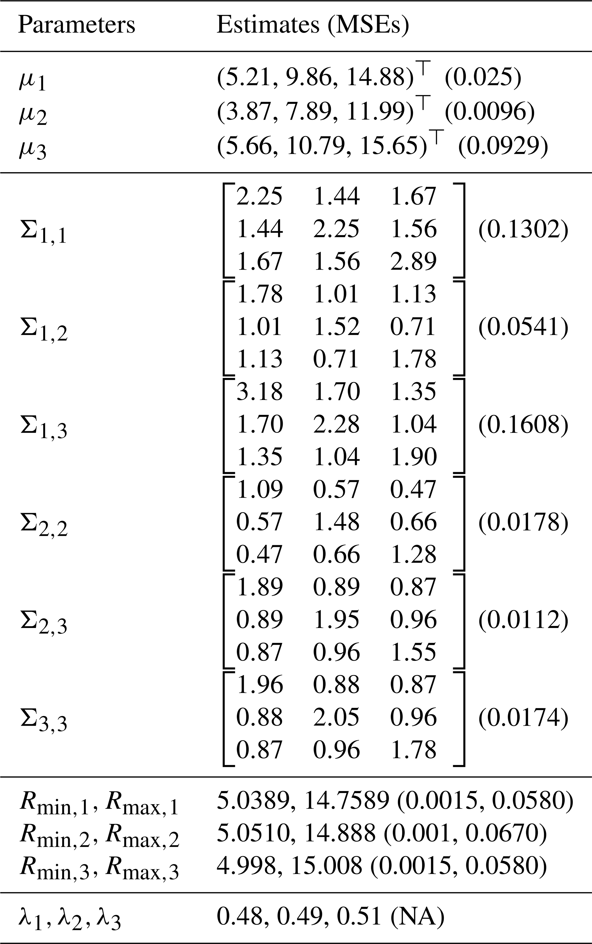
NA – no variation across simulations.

2.3 Asymptotic distribution of ML estimators for boxplot-valued data

In this subsection, we derive the asymptotic distribution of the ML estimators for the parameters of a boxplot-valued random variable.

Theorem 2. Let $\widehat{\mathit{\theta }}=(\widehat{\mathit{\mu }},\widehat{\mathbf{\Sigma }},\widehat{\mathit{\lambda }})$ denote the ML estimators for the parameters $\mathit{\theta }=(\mathit{\mu },\mathbf{\Sigma },\mathit{\lambda })$ of boxplot-valued data. Under regularity conditions (see, e.g., Ferguson, 2017), the asymptotic distribution of the ML estimators is given as

$$\sqrt{n}(\widehat{\mathit{\theta }}-\mathit{\theta })\stackrel{d}{\to }{\mathcal{N}}_{\frac{\mathrm{9}{p}^{\mathrm{2}}+\mathrm{11}p}{\mathrm{2}}}(\mathrm{0},\mathcal{I}(\mathit{\theta }{)}^{-\mathrm{1}}),$$

where ℐ(θ) is the Fisher information matrix and is given by

$$\mathcal{I}\left(\mathit{\theta }\right)=\left[\begin{array}{ccc}{\mathcal{I}}_{\mathit{\mu }}& \mathrm{0}& \mathrm{0}\\ \mathrm{0}& {\mathcal{I}}_{\mathbf{\Sigma }}& \mathrm{0}\\ \mathrm{0}& \mathrm{0}& {\mathcal{I}}_{\mathit{\lambda }}\end{array}\right]$$

with

$$\begin{array}{ll}{\displaystyle }{\mathcal{I}}_{\mathit{\mu }}& {\displaystyle }=n{\mathbf{I}}_{\mathrm{3}p}\otimes {\mathbf{\Sigma }}^{-\mathrm{1}},\\ {\displaystyle }{\mathcal{I}}_{\mathbf{\Sigma }}& {\displaystyle }={\displaystyle \frac{n}{\mathrm{2}}}({\mathbf{\Sigma }}^{-\mathrm{1}}\otimes {\mathbf{\Sigma }}^{-\mathrm{1}}),\\ {\displaystyle }{\mathcal{I}}_{\mathit{\lambda }}& {\displaystyle }=n\text{diag}\left({\displaystyle \frac{\mathrm{1}}{{\mathit{\lambda }}_{\mathrm{1}}^{\mathrm{2}}}},{\displaystyle \frac{\mathrm{1}}{{\mathit{\lambda }}_{\mathrm{2}}^{\mathrm{2}}}},\mathrm{\dots },{\displaystyle \frac{\mathrm{1}}{{\mathit{\lambda }}_p^{\mathrm{2}}}}\right),\end{array}$$

where I_3p is the 3p×3p identity matrix and ⊗ denotes the Kronecker product.

Proof. The Fisher information matrix is the expected value of the outer product of the score function $\mathrm{\nabla }\mathrm{\ell }\left(\mathit{\theta }\right)=\frac{\partial \mathrm{\ell }\left(\mathit{\theta }\right)}{\partial \mathit{\theta }}$, and it is given as

$$\mathcal{I}\left(\mathit{\theta }\right)=\mathbb{E}\left[\mathrm{\nabla }\mathrm{\ell }\left(\mathit{\theta }\right)\mathrm{\nabla }\mathrm{\ell }(\mathit{\theta }{)}^{\top }\right].$$

For the multivariate normal distribution ${\mathbf{Q}}_i\sim {\mathcal{N}}_{\mathrm{3}p}(\mathit{\mu },\mathbf{\Sigma })$, the score function for μ is

$${\displaystyle \frac{\partial \mathrm{\ell }}{\partial \mathit{\mu }}}={\mathbf{\Sigma }}^{-\mathrm{1}}\sum _{i=\mathrm{1}}^n({\mathbf{Q}}_i-\mathit{\mu }),$$

and hence

$${\mathcal{I}}_{\mathit{\mu }}=\mathbb{E}\left[\left({\displaystyle \frac{\partial \mathrm{\ell }}{\partial \mathit{\mu }}}\right){\left({\displaystyle \frac{\partial \mathrm{\ell }}{\partial \mathit{\mu }}}\right)}^{\top }\right]=n{\mathbf{I}}_{\mathrm{3}p}\otimes {\mathbf{\Sigma }}^{-\mathrm{1}}.$$

Similarly, for Σ, we have the score function

$${\displaystyle \frac{\partial \mathrm{\ell }}{\partial \mathbf{\Sigma }}}={\displaystyle \frac{\mathrm{1}}{\mathrm{2}}}\left({\mathbf{\Sigma }}^{-\mathrm{1}}-{\mathbf{\Sigma }}^{-\mathrm{1}}\mathbf{S}{\mathbf{\Sigma }}^{-\mathrm{1}}\right),$$

and therefore we have

$$\begin{array}{rl}{\mathcal{I}}_{\mathbf{\Sigma }}& ={\displaystyle \frac{n}{\mathrm{2}}}\mathbb{E}\left[{\mathbf{\Sigma }}^{-\mathrm{1}}\right({\mathbf{Q}}_i-\mathit{\mu }\left)\right({\mathbf{Q}}_i-\mathit{\mu }{)}^{\top }{\mathbf{\Sigma }}^{-\mathrm{1}}\\ & \otimes {\mathbf{\Sigma }}^{-\mathrm{1}}({\mathbf{Q}}_i-\mathit{\mu })({\mathbf{Q}}_i-\mathit{\mu }{)}^{\top }{\mathbf{\Sigma }}^{-\mathrm{1}}].\end{array}$$

Since $\mathbb{E}\left[({\mathbf{Q}}_i-\mathit{\mu })({\mathbf{Q}}_i-\mathit{\mu }{)}^{\top }\right]=\mathbf{\Sigma }$, we can write

$${\mathcal{I}}_{\mathbf{\Sigma }}={\displaystyle \frac{n}{\mathrm{2}}}({\mathbf{\Sigma }}^{-\mathrm{1}}\otimes {\mathbf{\Sigma }}^{-\mathrm{1}}).$$

For the uniform distribution $R_{ij}\sim \mathcal{U}(R_{\min ,j},R_{\max ,j})$, the Fisher information for the parameter λ_j (related to the range) is derived as

$${\mathcal{I}}_{\mathit{\lambda }}=n\text{diag}\left({\displaystyle \frac{\mathrm{1}}{{\mathit{\lambda }}_{\mathrm{1}}^{\mathrm{2}}}},{\displaystyle \frac{\mathrm{1}}{{\mathit{\lambda }}_{\mathrm{2}}^{\mathrm{2}}}},\mathrm{\dots },{\displaystyle \frac{\mathrm{1}}{{\mathit{\lambda }}_p^{\mathrm{2}}}}\right).$$

This expression reflects the dependence of the Fisher information on the individual λ_j values.

Using the central limit theorem, the score function evaluated at the true parameter values θ is asymptotically normally distributed as

$$\sqrt{n}\mathrm{\nabla }\mathrm{\ell }\left(\mathit{\theta }\right)\stackrel{d}{\to }{\mathcal{N}}_{\frac{\mathrm{9}{p}^{\mathrm{2}}+\mathrm{11}p}{\mathrm{2}}}(\mathrm{0},\mathcal{I}(\mathit{\theta }\left)\right).$$

The covariance of the score function is related to the Fisher information matrix by the information matrix equality

$$\mathrm{Cov}\left(\mathrm{\nabla }\mathrm{\ell }\right(\mathit{\theta }\left)\right)=\mathcal{I}\left(\mathit{\theta }\right).$$

The dimension of the parameter vector $\mathit{\theta }=(\mathit{\mu },\mathbf{\Sigma },\mathit{\lambda })$ is given by

$$\text{dim}\left(\mathit{\theta }\right)=\mathrm{3}p+{\displaystyle \frac{\mathrm{3}p(\mathrm{3}p+\mathrm{1})}{\mathrm{2}}}+p={\displaystyle \frac{\mathrm{9}{p}^{\mathrm{2}}+\mathrm{11}p}{\mathrm{2}}}.$$

This completes the proof.

□

3 Bayesian estimation for boxplot-valued data

Sadeghkhani and Sadeghkhani (2024) studied the Bayesian inference of symbolic interval-valued data by introducing noninformative priors, including the Jeffreys prior, into the multivariate setting. In this section, we use informative priors for boxplot-valued data, which allows us to update our prior knowledge based on the observed data. We derive the posterior distributions and find the Bayes estimators under the squared error loss (SEL) criterion.

3.1 Likelihood and priors

Consider the model where ${\mathit{Q}}_{\mathrm{1}},{\mathit{Q}}_{\mathrm{2}},\mathrm{\dots },{\mathit{Q}}_n$ are independent and identically distributed (iid) from 𝒩_3p(μ,Σ) with additional parameters R_minj, R_maxj, and λ_j for $j=\mathrm{1},\mathrm{2},\mathrm{\dots },p$ included in the likelihood function $\mathcal{L}(\mathit{\mu },\mathbf{\Sigma },\mathit{\{}{R}_{\min j}\mathit{\}},\mathit{\{}{R}_{\max j}\mathit{\}},\mathit{\{}{\mathit{\lambda }}_j\mathit{\}}\mid \mathit{Q})$.

We assume the following priors for the parameters:

$$\begin{array}{}\text{(19)}& {\displaystyle }\mathit{\mu }\mid \mathbf{\Sigma }& {\displaystyle }\sim {\mathcal{N}}_{\mathrm{3}p}({\mathit{\mu }}_{\mathrm{0}},\mathbf{\Sigma }/\mathit{\kappa }),\text{(20)}& {\displaystyle }\mathbf{\Sigma }& {\displaystyle }\sim {\mathcal{W}}_{\mathrm{3}p}^{-\mathrm{1}}({\mathit{\nu }}_{\mathrm{0}},{\mathrm{\Psi }}_{\mathrm{0}}),\end{array}$$

where μ₀ is the prior mean, κ is the scaling factor, ν₀ is the degrees of freedom, and Ψ₀ is the scale matrix of the inverse Wishart distribution. Additionally, we have

$$\begin{array}{}\text{(21)}& \begin{array}{rl}& R_{\min j}\sim \mathcal{U}(a_j,b_j),R_{\max j}\sim \mathcal{U}(c_j,d_j),\\ & {\mathit{\lambda }}_j\sim \mathcal{B}({\mathit{\alpha }}_j,{\mathit{\beta }}_j),\end{array}\end{array}$$

where $a_j,b_j,c_j,$ and d_j are the bounds of the uniform distributions and α_j and β_j are the parameters of the Beta distribution for each j.

Next, we find the posterior distributions of the parameters in the following lemma.

Lemma 1 (posterior distributions). Under the given priors in Eqs. (19), (20), and (21) and the observed data ${\mathit{Q}}_{\mathrm{1}},{\mathit{Q}}_{\mathrm{2}},\mathrm{\dots },{\mathit{Q}}_n$, we have the following.

• i.

  The posterior distribution of Σ is given by

  $$\begin{array}{}\text{(22)}& \mathbf{\Sigma }\mid \mathit{Q}\sim {\mathcal{W}}^{-\mathrm{1}}({\mathit{\nu }}_{\mathrm{0}}+n,{\mathbf{\Psi }}_{\mathrm{0}}+{\mathit{S}}_n),\end{array}$$

  where

  $${\mathit{S}}_n=\mathit{S}+{\displaystyle \frac{n\mathit{\kappa }}{n+\mathit{\kappa }}}(\stackrel{\mathrm{‾}}{\mathit{Q}}-{\mathit{\mu }}_{\mathrm{0}})(\stackrel{\mathrm{‾}}{\mathit{Q}}-{\mathit{\mu }}_{\mathrm{0}}{)}^{\top }$$

  and

  $$\mathit{S}=\sum _{i=\mathrm{1}}^n({\mathit{Q}}_i-\stackrel{\mathrm{‾}}{\mathit{Q}})({\mathit{Q}}_i-\stackrel{\mathrm{‾}}{\mathit{Q}}{)}^{\top },\stackrel{\mathrm{‾}}{\mathit{Q}}={\displaystyle \frac{\mathrm{1}}{n}}\sum _{i=\mathrm{1}}^n{\mathit{Q}}_i.$$
• ii.

  The posterior distribution of μ is

  $$\begin{array}{}\text{(23)}& \mathit{\mu }\mid \mathit{Q}\sim {\mathcal{T}}_{\mathrm{3}p}\left({\mathit{\mu }}_n,{\displaystyle \frac{{\mathrm{\Psi }}_{\mathrm{0}}+{\mathit{S}}_n}{\mathit{\kappa }(n+\mathit{\kappa })}}\left(\mathrm{1}+{\displaystyle \frac{\mathrm{1}}{n}}\right),{\mathit{\nu }}_{\mathrm{0}}+n-p+\mathrm{1}\right)\end{array}$$

  with

  $${\mathit{\mu }}_n={\displaystyle \frac{n\stackrel{\mathrm{‾}}{\mathit{Q}}+\mathit{\kappa }{\mathit{\mu }}_{\mathrm{0}}}{n+\mathit{\kappa }}},$$

  where ${\mathcal{T}}_p(\mathit{m},\mathit{A},\mathit{\nu })$ represents a multivariate Student's t distribution with mean vector m, variance matrix A, and ν degrees of freedom.

• iii.

  The posterior distribution of R_minj is given by

  $$R_{\min j}\mid \mathit{Q}\sim \mathcal{U}(max(a_j,R_{\min j,\text{obs}}),b_j),$$

  where R_minj,obs is the minimum observed R_minj.

• iv.

  The posterior distribution of R_maxj is given by

  $$R_{\max j}\mid \mathit{Q}\sim \mathcal{U}(c_j,\min (d_j,R_{\max j,\text{obs}}\left)\right),$$

  where R_maxj,obs is the maximum observed R_maxj.

• v.

  The posterior distribution of λ_j is given by

  $${\mathit{\lambda }}_j\mid \mathit{Q}\sim \mathcal{B}({\mathit{\alpha }}_j+n,{\mathit{\beta }}_j+n).$$

Proof. According to Bayes' rule, the posterior distributions are derived as follows:

• i.

  The posterior of Σ is given by

  $$\begin{array}{rl}\mathit{\pi }(\mathbf{\Sigma }\mid \mathit{Q})& \propto \mathcal{L}(\mathit{\mu },\mathbf{\Sigma },\mathit{\{}{R}_{\min j}\mathit{\}},\mathit{\{}{R}_{\max j}\mathit{\}},\mathit{\{}{\mathit{\lambda }}_j\mathit{\}}\mid \mathit{Q})\mathit{\pi }\left(\mathbf{\Sigma }\right)\\ & \propto |\mathbf{\Sigma }{|}^{-\frac{n}{\mathrm{2}}}\exp \left(-{\displaystyle \frac{\mathrm{1}}{\mathrm{2}}}\sum _{i=\mathrm{1}}^n({\mathit{Q}}_i-\mathit{\mu }{)}^{\top }{\mathbf{\Sigma }}^{-\mathrm{1}}({\mathit{Q}}_i-\mathit{\mu })\right)\\ & \times |\mathbf{\Sigma }{|}^{-({\mathit{\nu }}_{\mathrm{0}}+\mathrm{3}p+\mathrm{1})/\mathrm{2}}\exp \left(-{\displaystyle \frac{\mathrm{1}}{\mathrm{2}}}\mathrm{tr}\left({\mathrm{\Psi }}_{\mathrm{0}}{\mathbf{\Sigma }}^{-\mathrm{1}}\right)\right)\\ & \propto |\mathbf{\Sigma }{|}^{-({\mathit{\nu }}_{\mathrm{0}}+n+\mathrm{3}p+\mathrm{1})/\mathrm{2}}\exp \left(-{\displaystyle \frac{\mathrm{1}}{\mathrm{2}}}\mathrm{tr}\left(({\mathrm{\Psi }}_{\mathrm{0}}+{\mathit{S}}_n){\mathbf{\Sigma }}^{-\mathrm{1}}\right)\right),\end{array}$$

  which is the kernel of an inverse Wishart distribution:

  $$\mathbf{\Sigma }\mid \mathit{Q}\sim {\mathcal{W}}^{-\mathrm{1}}({\mathit{\nu }}_{\mathrm{0}}+n,{\mathbf{\Psi }}_{\mathrm{0}}+{\mathit{S}}_n).$$
• ii.

  The posterior of μ is given by

  $$\begin{array}{rl}\mathit{\pi }(\mathit{\mu }\mid \mathit{Q},\mathbf{\Sigma })& \propto \mathcal{L}(\mathit{\mu },\mathbf{\Sigma }\mid \mathit{Q})\mathit{\pi }(\mathit{\mu }\mid \mathbf{\Sigma })\\ & \propto \exp \left(-{\displaystyle \frac{\mathrm{1}}{\mathrm{2}}}\sum _{i=\mathrm{1}}^n({\mathit{Q}}_i-\mathit{\mu }{)}^{\top }{\mathbf{\Sigma }}^{-\mathrm{1}}({\mathit{Q}}_i-\mathit{\mu })\right)\\ & \times \exp \left(-{\displaystyle \frac{\mathrm{1}}{\mathrm{2}}}(\mathit{\mu }-{\mathit{\mu }}_{\mathrm{0}}{)}^{\top }{\left({\displaystyle \frac{\mathit{\kappa }}{\mathbf{\Sigma }}}\right)}^{-\mathrm{1}}(\mathit{\mu }-{\mathit{\mu }}_{\mathrm{0}})\right)\\ & \propto \exp \left(-{\displaystyle \frac{\mathrm{1}}{\mathrm{2}}}(\mathit{\mu }-{\mathit{\mu }}_n{)}^{\top }{\left({\displaystyle \frac{\mathrm{1}}{n+\mathit{\kappa }}}\mathbf{\Sigma }+{\displaystyle \frac{\mathit{\kappa }}{\mathbf{\Sigma }}}\right)}^{-\mathrm{1}}(\mathit{\mu }-{\mathit{\mu }}_n)\right),\end{array}$$

  which results in a multivariate normal distribution for μ given Σ, i.e.,

  $$\mathit{\mu }\mid \mathit{Q},\mathbf{\Sigma }\sim {\mathcal{N}}_{\mathrm{3}p}\left({\mathit{\mu }}_n,{\displaystyle \frac{\mathbf{\Sigma }}{n+\mathit{\kappa }}}\right).$$

  By integrating out Σ, we have

  $$\mathit{\mu }\mid \mathit{Q}\sim {\mathcal{T}}_{\mathrm{3}p}\left({\mathit{\mu }}_n,{\displaystyle \frac{{\mathrm{\Psi }}_{\mathrm{0}}+{\mathit{S}}_n}{\mathit{\kappa }(n+\mathit{\kappa })}}\left(\mathrm{1}+{\displaystyle \frac{\mathrm{1}}{n}}\right),{\mathit{\nu }}_{\mathrm{0}}+n-p+\mathrm{1}\right).$$
• iii.

  For R_minj, combining the likelihood with the uniform prior results in the posterior distribution

  $$R_{\min j}\mid \mathit{Q}\sim \mathcal{U}(max(a_j,R_{\min j,\text{obs}}),b_j).$$
• iv.

  For R_maxj, combining the likelihood with the uniform prior results in the posterior distribution

  $$R_{\max j}\mid \mathit{Q}\sim \mathcal{U}(c_j,\min (d_j,R_{\max j,\text{obs}}\left)\right).$$
• v.

  For λ_j, combining the likelihood with the Beta prior results in the posterior distribution

  $${\mathit{\lambda }}_j\mid \mathit{Q}\sim \mathcal{B}({\mathit{\alpha }}_j+n,{\mathit{\beta }}_j+n).$$

□

Next, Theorem 3 provides the Bayes estimator of unknown parameters of a boxplot-valued random variable.

Theorem 3 (Bayes estimators under SEL). Under the assumptions of Lemma 1, the Bayes estimators under SEL, which are the means of the marginal posteriors, are obtained as follows:

• i.

  The Bayes estimator of μ is

  $$\begin{array}{}\text{(24)}& {\widehat{\mathit{\mu }}}_{\text{Bayes}}={\displaystyle \frac{n\stackrel{\mathrm{‾}}{\mathit{Q}}+\mathit{\kappa }{\mathit{\mu }}_{\mathrm{0}}}{n+\mathit{\kappa }}}.\end{array}$$
• ii.

  The Bayes estimator of Σ is

  $${\widehat{\mathbf{\Sigma }}}_{\text{Bayes}}={\displaystyle \frac{{\mathrm{\Psi }}_{\mathrm{0}}+{\mathit{S}}_n}{{\mathit{\nu }}_{\mathrm{0}}+n-\mathrm{3}p-\mathrm{1}}},$$

  where

  $${\mathit{S}}_n=\mathit{S}+{\displaystyle \frac{n\mathit{\kappa }}{n+\mathit{\kappa }}}(\stackrel{\mathrm{‾}}{\mathit{Q}}-{\mathit{\mu }}_{\mathrm{0}})(\stackrel{\mathrm{‾}}{\mathit{Q}}-{\mathit{\mu }}_{\mathrm{0}}{)}^{\top }$$

  and

  $$\mathit{S}=\sum _{i=\mathrm{1}}^n({\mathit{Q}}_i-\stackrel{\mathrm{‾}}{\mathit{Q}})({\mathit{Q}}_i-\stackrel{\mathrm{‾}}{\mathit{Q}}{)}^{\top },\stackrel{\mathrm{‾}}{\mathit{Q}}={\displaystyle \frac{\mathrm{1}}{n}}\sum _{i=\mathrm{1}}^n{\mathit{Q}}_i.$$
• iii.

  The Bayes estimators of R_minj and R_maxj are

  $$\begin{array}{rl}& {\widehat{R}}_{\min j,\text{Bayes}}={\displaystyle \frac{max(a_j,R_{\min j,\text{obs}})+b_j}{\mathrm{2}}},\\ & {\widehat{R}}_{\max j,\text{Bayes}}={\displaystyle \frac{c_j+\min (d_j,R_{\max j,\text{obs}})}{\mathrm{2}}},\end{array}$$

  where R_minj,obs and R_maxj,obs are the minimum observed R_minj and maximum observed R_maxj, respectively.

• iv.

  The Bayes estimator of λ_j is

  $${\widehat{\mathit{\lambda }}}_{\text{Bayes}}={\displaystyle \frac{{\mathit{\alpha }}_j+n}{{\mathit{\alpha }}_j+{\mathit{\beta }}_j+\mathrm{2}n}}.$$

Proof. The Bayes estimators are the means of the posterior distributions given in Lemma 1, and this completes the proof.

□

3.2 Simulation study in the Bayesian setup

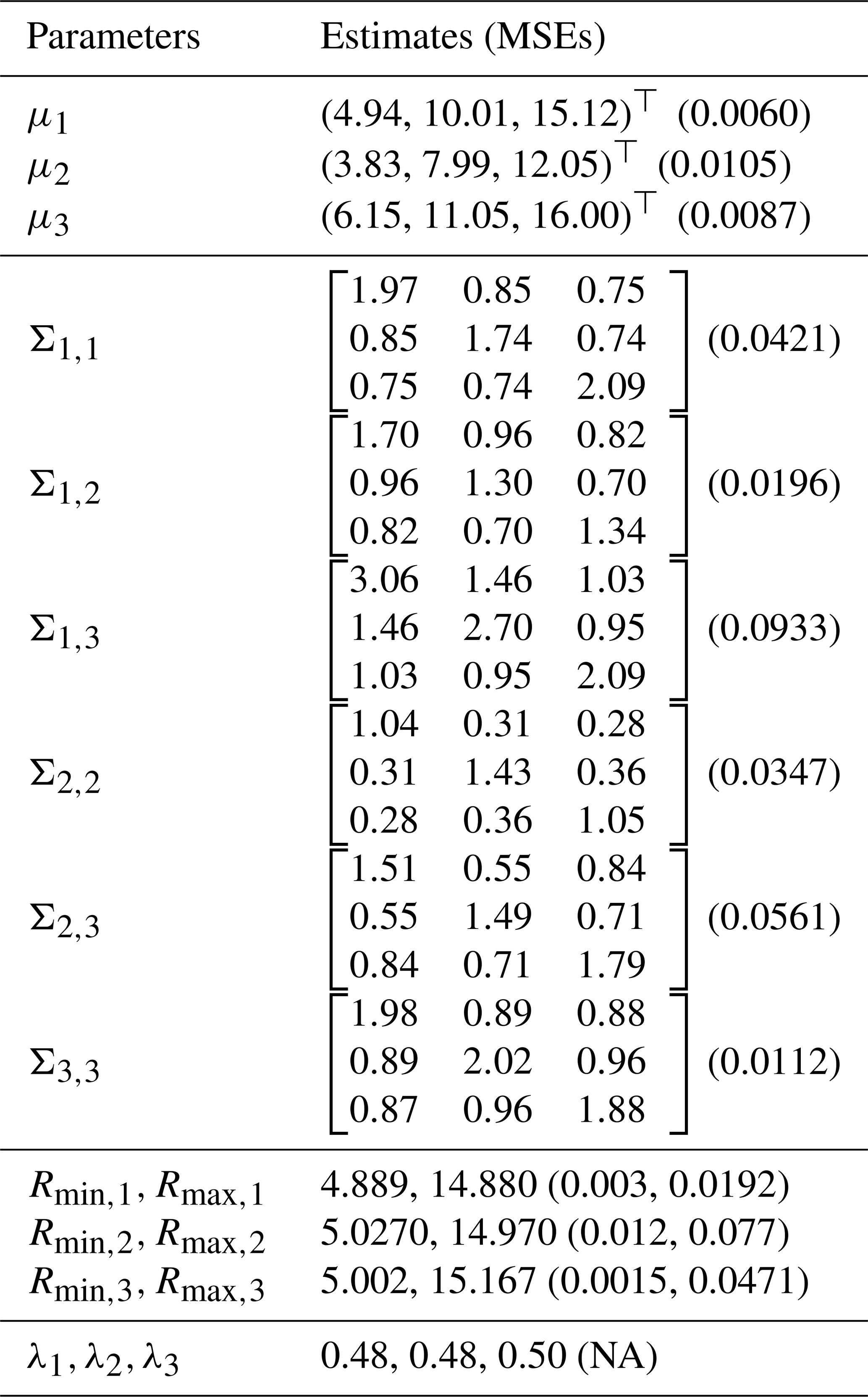
Similar to Sect. 2.2, we conduct a simulation study to demonstrate the Bayesian estimation procedure. The simulation is carried out with the same setup and true values as described there, i.e., for p=3 variables with a sample size of n=100 and the true parameters specified in Eqs. (15)–(17).

Here, we use noninformative priors to ensure that the data predominantly influence the parameter estimates. In this simulation, a normal prior distribution with mean vector 0 and covariance matrix 10² I_p is used for μ. An inverse Wishart prior distribution is employed for Σ with a scale matrix S₀=I_p and degrees of freedom $\mathit{\nu }=p+\mathrm{1}$. For each λ_j, $j=\mathrm{1},\mathrm{2},\mathrm{3}$ a uniform 𝒰(0,1) ($\mathcal{B}({\mathit{\alpha }}_j=\mathrm{1},{\mathit{\beta }}_j=\mathrm{1})$) is used, which covers a broad range of values to avoid imposing any strong constraints.

The results of the Bayesian estimation, including the MSEs for each parameter, are summarized in Table 2.

Table 2 Bayesian estimates and MSEs.

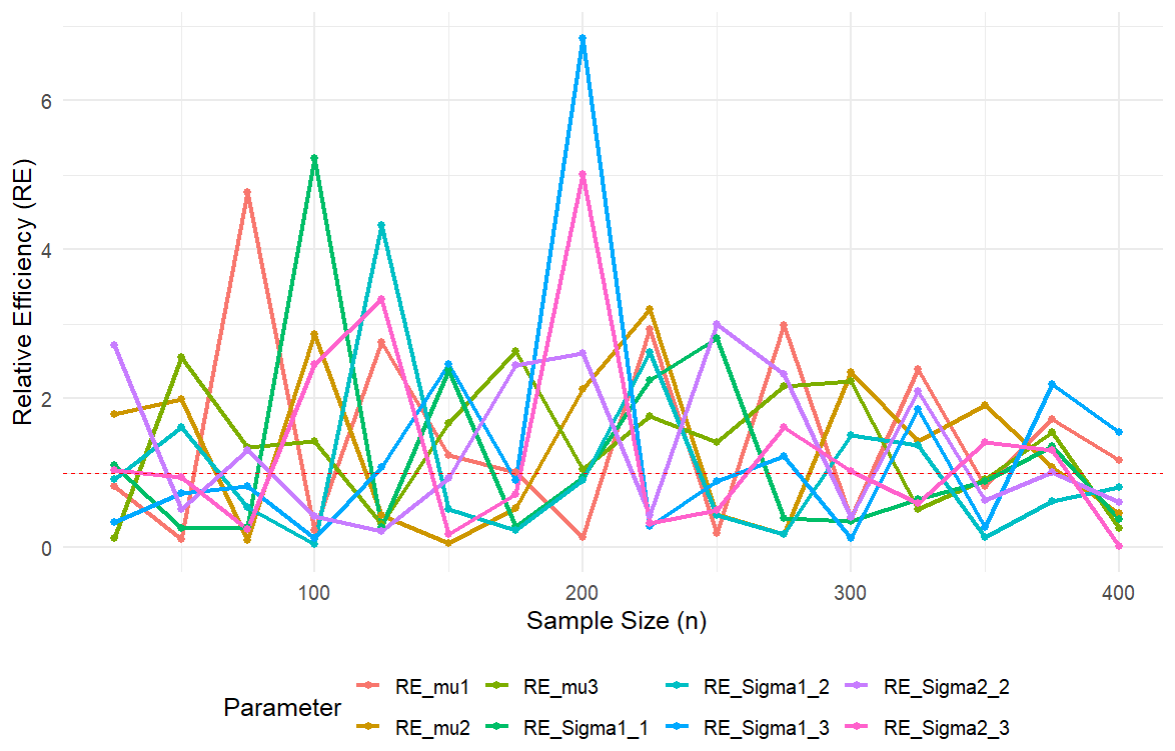
In order to compare the efficiency of the proposed ML and Bayesian estimators for different sample sizes n, we use the same simulation settings as those in Sects. 2.2 and 3.2. Figure 1 illustrates the relative efficiency (RE), defined as the MSE of the ML estimator over the MSE of the Bayesian estimator for the parameters μ and Σ. It can be seen that, for smaller sample sizes n, the efficiency of the Bayesian estimators is generally better (RE > 1). As n increases, thanks to the consistency of the ML estimators, the ML estimators tend to outperform the Bayesian estimators (RE < 1).

Figure 1 Relative efficiency of Bayesian and ML estimators in the simulation study (Sects. 2.2 and 3.2).

4 Posterior predictive density estimator

Given the posterior distributions of the parameters μ, Σ, λ_j, R_minj, and R_maxj derived in Lemma 1, we can obtain the posterior predictive density for a new observation Q^*. Theorem 4 finds the posterior predictive density estimator for a future or new random variable Q^*.

Theorem 4 (posterior predictive density estimator). The posterior predictive density for a new random variable Q^* given the observable ${\mathbf{Q}}_{\mathrm{1}},\mathrm{\dots },{\mathbf{Q}}_n$ is as follows:

• i.

  When λ_j is known, the posterior predictive density estimator is given by

  $$\begin{array}{}\text{(25)}& \begin{array}{rl}& {\mathbf{Q}}^{*}\mid {\mathbf{Q}}_{\mathrm{1}},\mathrm{\dots },{\mathbf{Q}}_n\\ & \sim {\mathcal{T}}_{\mathrm{3}p}({\displaystyle \frac{\mathit{\kappa }{\mathit{\mu }}_{\mathrm{0}}+n\stackrel{\mathrm{‾}}{\mathbf{Q}}}{\mathit{\kappa }+n}},{\displaystyle \frac{(\mathit{\kappa }+n+\mathrm{1})({\mathrm{\Psi }}_{\mathrm{0}}+{\mathit{S}}_n/{\mathit{\lambda }}_j)}{(\mathit{\kappa }+n)({\mathit{\nu }}_{\mathrm{0}}+n-\mathrm{3}p+\mathrm{1})}},\\ & {\mathit{\nu }}_{\mathrm{0}}+n-\mathrm{3}p+\mathrm{1}).\end{array}\end{array}$$
• ii.

  When λ_j is unknown, the posterior predictive density is a mixture of multivariate Student's t distributions as given by

  $$\begin{array}{}\text{(26)}& \begin{array}{rl}& p({\mathbf{Q}}^{*}\mid {\mathbf{Q}}_{\mathrm{1}},\mathrm{\dots },{\mathbf{Q}}_n)\\ & =\int {\mathcal{T}}_{\mathrm{3}p}({\displaystyle \frac{\mathit{\kappa }{\mathit{\mu }}_{\mathrm{0}}+n\stackrel{\mathrm{‾}}{\mathbf{Q}}}{\mathit{\kappa }+n}},{\displaystyle \frac{(\mathit{\kappa }+n+\mathrm{1})({\mathrm{\Psi }}_{\mathrm{0}}+\frac{\mathrm{1}}{{\mathit{\lambda }}_j}{\mathit{S}}_n)}{(\mathit{\kappa }+n)({\mathit{\nu }}_{\mathrm{0}}+n-\mathrm{3}p+\mathrm{1})}},\\ & {\mathit{\nu }}_{\mathrm{0}}+n-\mathrm{3}p+\mathrm{1})\times p({\mathit{\lambda }}_j\mid {\mathbf{Q}}_{\mathrm{1}},\mathrm{\dots },{\mathbf{Q}}_n)\mathrm{d}{\mathit{\lambda }}_j.\end{array}\end{array}$$

Proof. To derive the posterior predictive density, we need to integrate the parameters μ, Σ, and λ_j from the joint posterior distribution:

• i.

  When λ_j is known, from Lemma 1, the posterior distributions of μ and Σ are given by

  $$\begin{array}{c}{\displaystyle }\mathit{\mu }\mid \mathbf{\Sigma },\mathbf{Q}\sim {\mathcal{N}}_{\mathrm{3}p}\left({\displaystyle \frac{\mathit{\kappa }{\mathit{\mu }}_{\mathrm{0}}+n\stackrel{\mathrm{‾}}{\mathbf{Q}}}{\mathit{\kappa }+n}},{\displaystyle \frac{\mathbf{\Sigma }}{\mathit{\kappa }+n}}\right),\\ {\displaystyle }\mathbf{\Sigma }\mid \mathbf{Q}\sim {\mathcal{W}}_{\mathrm{3}p}^{-\mathrm{1}}({\mathit{\nu }}_{\mathrm{0}}+n,{\mathrm{\Psi }}_{\mathrm{0}}+{\mathit{S}}_n),\end{array}$$

  and therefore the posterior predictive density is given by

  $$\begin{array}{rl}& p({\mathbf{Q}}^{*}\mid {\mathbf{Q}}_{\mathrm{1}},\mathrm{\dots },{\mathbf{Q}}_n)\\ & =\int \int p({\mathbf{Q}}^{*}\mid \mathit{\mu },\mathbf{\Sigma })p(\mathit{\mu },\mathbf{\Sigma }\mid {\mathbf{Q}}_{\mathrm{1}},\mathrm{\dots },{\mathbf{Q}}_n)\mathrm{d}\mathit{\mu }\mathrm{d}\mathbf{\Sigma }.\end{array}$$

  Since $p(\mathit{\mu },\mathbf{\Sigma }\mid {\mathbf{Q}}_{\mathrm{1}},\mathrm{\dots },{\mathbf{Q}}_n)$ follows a normal inverse Wishart distribution, the resulting predictive density is a multivariate Student's t distribution:

  $$\begin{array}{rl}& {\mathbf{Q}}^{*}\mid {\mathbf{Q}}_{\mathrm{1}},\mathrm{\dots },{\mathbf{Q}}_n\\ & \sim {\mathcal{T}}_{\mathrm{3}p}({\displaystyle \frac{\mathit{\kappa }{\mathit{\mu }}_{\mathrm{0}}+n\stackrel{\mathrm{‾}}{\mathbf{Q}}}{\mathit{\kappa }+n}},{\displaystyle \frac{(\mathit{\kappa }+n+\mathrm{1})({\mathrm{\Psi }}_{\mathrm{0}}+{\mathit{S}}_n)}{(\mathit{\kappa }+n)({\mathit{\nu }}_{\mathrm{0}}+n-\mathrm{3}p+\mathrm{1})}},\\ & {\mathit{\nu }}_{\mathrm{0}}+n-\mathrm{3}p+\mathrm{1}).\end{array}$$
• ii.

  When λ_j is unknown, the posterior distributions of μ, Σ, and λ_j are

  $$\begin{array}{ll}{\displaystyle }\mathit{\mu }& {\displaystyle }\mid \mathbf{\Sigma },{\mathit{\lambda }}_j,\mathbf{Q}\sim {\mathcal{N}}_{\mathrm{3}p}\left({\displaystyle \frac{\mathit{\kappa }{\mathit{\mu }}_{\mathrm{0}}+n\stackrel{\mathrm{‾}}{\mathbf{Q}}}{\mathit{\kappa }+n}},{\displaystyle \frac{\mathbf{\Sigma }}{{\mathit{\lambda }}_j(\mathit{\kappa }+n)}}\right),\\ {\displaystyle }\mathbf{\Sigma }& {\displaystyle }\mid {\mathit{\lambda }}_j,\mathbf{Q}\sim {\mathcal{W}}_{\mathrm{3}p}^{-\mathrm{1}}\left({\mathit{\nu }}_{\mathrm{0}}+n,{\mathrm{\Psi }}_{\mathrm{0}}+{\displaystyle \frac{\mathrm{1}}{{\mathit{\lambda }}_j}}{\mathit{S}}_n\right),\\ {\displaystyle }{\mathit{\lambda }}_j& {\displaystyle }\mid \mathbf{Q}\sim p({\mathit{\lambda }}_j\mid {\mathbf{Q}}_{\mathrm{1}},\mathrm{\dots },{\mathbf{Q}}_n).\end{array}$$

  Then, the posterior predictive density is given by

  $$\begin{array}{rl}& p({\mathbf{Q}}^{*}\mid {\mathbf{Q}}_{\mathrm{1}},\mathrm{\dots },{\mathbf{Q}}_n)\\ & =\int \int \int p({\mathbf{Q}}^{*}\mid \mathit{\mu },\mathbf{\Sigma },{\mathit{\lambda }}_j)p(\mathit{\mu },\mathbf{\Sigma },{\mathit{\lambda }}_j\mid {\mathbf{Q}}_{\mathrm{1}},\mathrm{\dots },{\mathbf{Q}}_n)\\ & \cdot \mathrm{d}\mathit{\mu }\mathrm{d}\mathbf{\Sigma }\mathrm{d}{\mathit{\lambda }}_j,\end{array}$$

  and this completes the proof.

□

Remark 1. In addition to the posterior predictive density derived in Theorem 4, two other types of density estimators can be considered: plugin density estimators. We assume that λ is known or has been estimated using either Bayesian or ML methods.

• i.

  ML plugin density estimator: by plugging in the ML estimators for μ, Σ, and λ from Theorem 2, the density estimator is given by

  $$p({\mathbf{Q}}^{*}\mid \widehat{\mathit{\mu }},\widehat{\mathbf{\Sigma }},\widehat{\mathit{\lambda }})={\mathcal{N}}_{\mathrm{3}p}(\widehat{\mathit{\mu }},\widehat{\mathbf{\Sigma }}).$$
• ii.

  Bayesian plugin density estimator: by plugging in the Bayesian estimators for μ, Σ, and λ from Theorem 3, the density estimator is

  $$p({\mathbf{Q}}^{*}\mid {\widehat{\mathit{\mu }}}_{\text{Bayes}},{\widehat{\mathbf{\Sigma }}}_{\text{Bayes}},{\widehat{\mathit{\lambda }}}_{\text{Bayes}})={\mathcal{N}}_{\mathrm{3}p}({\widehat{\mathit{\mu }}}_{\text{Bayes}},{\widehat{\mathbf{\Sigma }}}_{\text{Bayes}}).$$

  Note that, in both cases, λ influences the range but not the normal distribution part.

4.1 Comparison of density estimators using the expected Kullback–Leibler (KL) Loss

The KL loss function measures the difference between two probability distributions. For a true density p(Q) and an estimated density q(Q), the KL loss is defined as

$$\begin{array}{}\text{(27)}& D_{\text{KL}}(p\Vert q)=\int p\left(\mathbf{Q}\right)\log \left({\displaystyle \frac{p\left(\mathbf{Q}\right)}{q\left(\mathbf{Q}\right)}}\right)\mathrm{d}\mathbf{Q}.\end{array}$$

The expected KL loss, also known as the KL risk function, for a density estimator q is the expectation of KL loss over the distribution of the data and is given as

$$\begin{array}{}\text{(28)}& R_{\text{KL}}\left(q\right)=\mathbb{E}\left[D_{\text{KL}}(p\Vert q)\right].\end{array}$$

To evaluate the performance of different predictive density estimators, we compare the KL risk performance of three methods in estimating the future density, i.e., Bayesian predictive, Bayesian plugin, and ML plugin estimators. The next lemma helps to find the KL risk functions.

Lemma 2. The KL loss between two multivariate normal distributions 𝒩_p(μ₁,Σ₁) and 𝒩_p(μ₂,Σ₂) is given by

$$\begin{array}{rl}& \text{KL}\left({\mathcal{N}}_p\right({\mathit{\mu }}_{\mathrm{1}},{\mathbf{\Sigma }}_{\mathrm{1}})\parallel {\mathcal{N}}_p({\mathit{\mu }}_{\mathrm{2}},{\mathbf{\Sigma }}_{\mathrm{2}}\left)\right)\\ & ={\displaystyle \frac{\mathrm{1}}{\mathrm{2}}}\left[\text{tr}\right({\mathbf{\Sigma }}_{\mathrm{2}}^{-\mathrm{1}}{\mathbf{\Sigma }}_{\mathrm{1}})+({\mathit{\mu }}_{\mathrm{2}}-{\mathit{\mu }}_{\mathrm{1}}{)}^{\top }{\mathbf{\Sigma }}_{\mathrm{2}}^{-\mathrm{1}}({\mathit{\mu }}_{\mathrm{2}}-{\mathit{\mu }}_{\mathrm{1}})\\ & -p+\log {\displaystyle \frac{\det \left({\mathbf{\Sigma }}_{\mathrm{2}}\right)}{\det \left({\mathbf{\Sigma }}_{\mathrm{1}}\right)}}].\end{array}$$

The KL divergence between a multivariate normal distribution and a multivariate Student's t distribution is given by

$$\begin{array}{rl}& \text{KL}\left({\mathcal{N}}_p\right({\mathit{\mu }}_{\mathrm{1}},{\mathbf{\Sigma }}_{\mathrm{1}})\parallel {\mathcal{T}}_p({\mathit{\mu }}_{\mathrm{2}},{\mathbf{\Sigma }}_{\mathrm{2}},\mathit{\nu }\left)\right)\\ & ={\displaystyle \frac{\mathrm{1}}{\mathrm{2}}}\left[\text{tr}\right({\mathbf{\Sigma }}_{\mathrm{1}}^{-\mathrm{1}}{\mathbf{\Sigma }}_{\mathrm{2}})+({\mathit{\mu }}_{\mathrm{2}}-{\mathit{\mu }}_{\mathrm{1}}{)}^{\top }{\mathbf{\Sigma }}_{\mathrm{1}}^{-\mathrm{1}}({\mathit{\mu }}_{\mathrm{2}}-{\mathit{\mu }}_{\mathrm{1}})\\ & -p+\log {\displaystyle \frac{\det \left({\mathbf{\Sigma }}_{\mathrm{2}}\right)}{\det \left({\mathbf{\Sigma }}_{\mathrm{1}}\right)}}]-{\displaystyle \frac{p}{\mathrm{2}}}\left({\displaystyle \frac{\mathit{\nu }-p+\mathrm{1}}{\mathit{\nu }}}\right),\end{array}$$

where tr(⋅) denotes the trace of a given matrix.

Proof. The KL loss function between two multivariate normal densities is straightforward and therefore omitted. Given the density function of the multivariate normal distribution as

$$p\left(\mathbf{Q}\right)={\displaystyle \frac{\mathrm{1}}{\left(\mathrm{2}\mathit{\pi }{)}^{p/\mathrm{2}}\right|{\mathbf{\Sigma }}_{\mathrm{1}}{|}^{\mathrm{1}/\mathrm{2}}}}\exp \left(-{\displaystyle \frac{\mathrm{1}}{\mathrm{2}}}(\mathbf{Q}-{\mathit{\mu }}_{\mathrm{1}}{)}^{\top }{\mathbf{\Sigma }}_{\mathrm{1}}^{-\mathrm{1}}(\mathbf{Q}-{\mathit{\mu }}_{\mathrm{1}})\right)$$

and the density function of the multivariate Student's t distribution as

$$\begin{array}{rl}q\left(\mathbf{Q}\right)& ={\displaystyle \frac{\mathrm{\Gamma }\left(\frac{\mathit{\nu }+p}{\mathrm{2}}\right)}{\mathrm{\Gamma }\left(\frac{\mathit{\nu }}{\mathrm{2}}\right)\left(\mathit{\nu }\mathit{\pi }{)}^{p/\mathrm{2}}\right|{\mathbf{\Sigma }}_{\mathrm{2}}{|}^{\mathrm{1}/\mathrm{2}}}}\\ & \cdot {\left(\mathrm{1}+{\displaystyle \frac{\mathrm{1}}{\mathit{\nu }}}(\mathbf{Q}-{\mathit{\mu }}_{\mathrm{2}}{)}^{\top }{\mathbf{\Sigma }}_{\mathrm{2}}^{-\mathrm{1}}(\mathbf{Q}-{\mathit{\mu }}_{\mathrm{2}})\right)}^{-\frac{\mathit{\nu }+p}{\mathrm{2}}},\end{array}$$

substituting these into the KL loss function in Eq. (27) and simplifying them gives the result.

□

4.1.1 KL risk function comparison simulation

We conducted a simulation study to evaluate the KL risk for different sample sizes using three methods: Bayesian predictive, Bayesian plugin, and ML plugin estimators. The true parameters and hyperparameters used in the simulation are as follows. The true parameters are defined as

$$\mathit{\mu }=\left[\begin{array}{c}\mathrm{1}\\ \mathrm{2}\\ \mathrm{3}\end{array}\right],\mathbf{\Sigma }=\left[\begin{array}{ccc}\mathrm{1}& \mathrm{0.5}& \mathrm{0.3}\\ \mathrm{0.5}& \mathrm{2}& \mathrm{0.4}\\ \mathrm{0.3}& \mathrm{0.4}& \mathrm{3}\end{array}\right],$$

and the prior parameters are defined as

$${\mathit{\mu }}_{\mathrm{0}}=\left[\begin{array}{c}\mathrm{0}\\ \mathrm{0}\\ \end{array}\right],{\mathit{\kappa }}_{\mathrm{0}}=\mathrm{0.0001},{\mathit{\nu }}_{\mathrm{0}}=\mathrm{3},{\mathbf{\Psi }}_{\mathrm{0}}=\left[\begin{array}{ccc}\mathrm{1}& \mathrm{0}& \mathrm{0}\\ \mathrm{0}& \mathrm{1}& \mathrm{0}\\ \mathrm{0}& \mathrm{0}& \mathrm{1}\end{array}\right].$$

Table 3 KL risk comparison of different density estimators with different sample sizes.

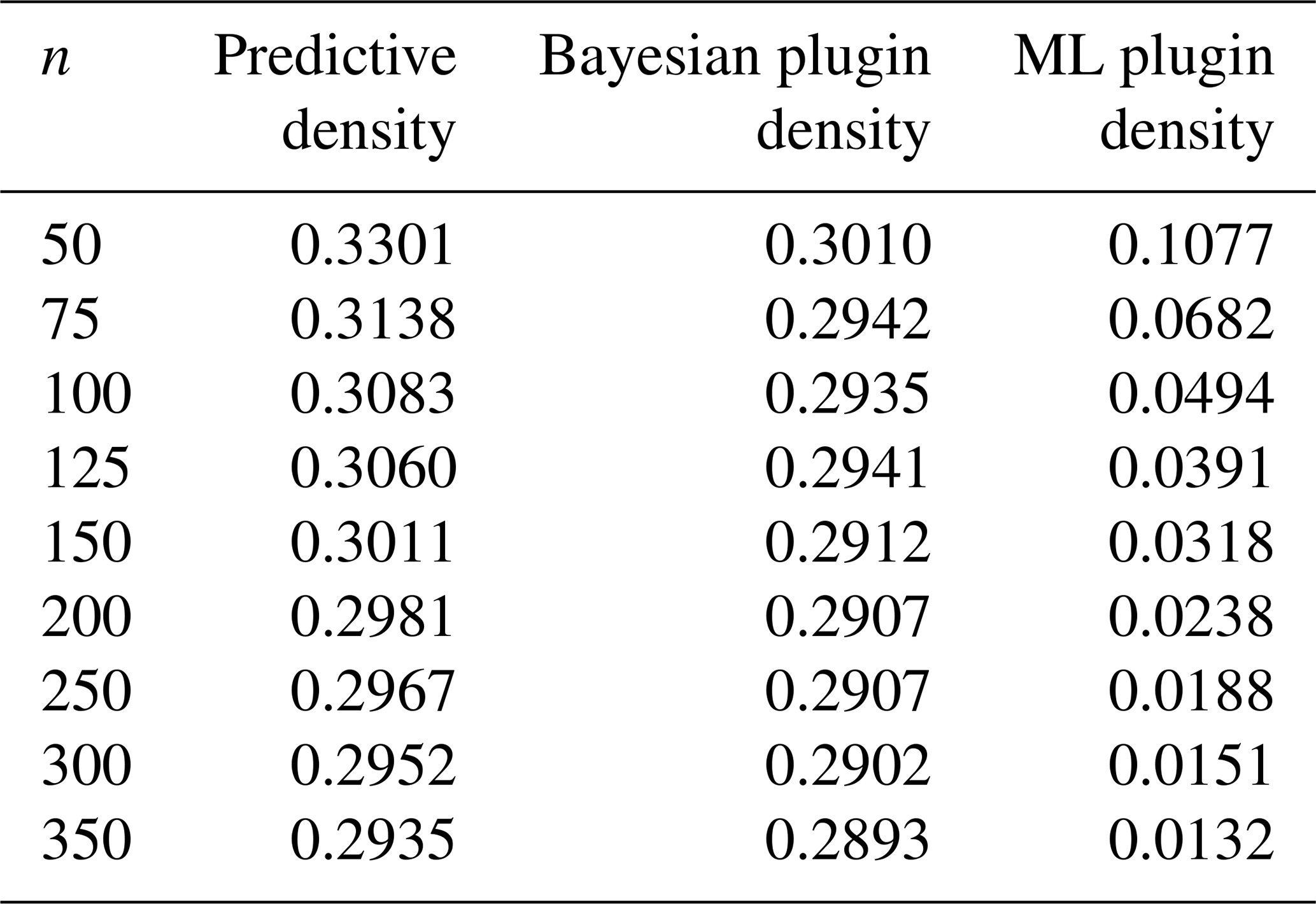
As seen from Table 3 and Fig. 2, the KL risks for the Bayesian predictive and plugin density estimators are quite close. Both risk functions are fairly small, and the difference between them decreases as the sample size n increases. Moreover, the KL risk for the ML plugin density estimator is smaller than that for the other two estimators, and it decreases as n increases. This suggests that the ML plugin density estimator performs better when estimating the new density. However, it is important to note that both Bayesian estimators were based on noninformative priors by choosing a very small value for κ₀.

To visualize the comparison of KL divergence for different sample sizes, we present a plot in Fig. 2.

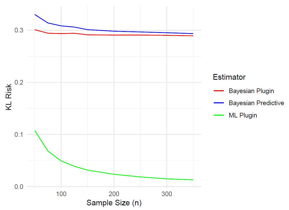
Figure 2 KL risk function comparison of different density estimators for different sample sizes.

5 Applications in climatology

In this section, we apply the methodologies discussed – specifically the point estimation methods (both ML and Bayesian) and density estimations – to real climatological data. This approach demonstrates the practical utility and effectiveness of these statistical techniques in analyzing and interpreting complex boxplot-valued environmental data. The data are sourced from the Berkeley Earth Surface Temperature Study, which aggregates 1.6 billion temperature reports from 16 pre-existing archives affiliated with the Lawrence Berkeley National Laboratory (data can be found in the Berkeley Earth Surface Temperature Study at https://www.kaggle.com/berkeleyearth/climate-change-earth-surface-temperature-data, last access: 19 July 2024).

The section is divided into two subsections, each focusing on a distinct aspect of climatological analysis. First, we examine the monthly average temperatures in the United States from January 2000 to September 2013. In the latter subsection, we analyze summer average temperatures in European countries, with data going back to the 18th century. Both datasets are vast, containing extensive data. Aggregating these data into boxplots allows for computational efficiency by representing large amounts of information in a concise form.

5.1 Analysis of monthly average temperatures in the United States

5.1.1 Point estimators

The dataset used for this analysis includes monthly average temperatures from various cities across the United States, spanning from January 2000 to September 2013. These extensive data provide a comprehensive view of temperature trends and variations over a significant period. Here, each X_i represents the monthly average temperature summaries across multiple cities for month i within this period, capturing the variability of average temperatures in the form of symbolic data.

For each month, the first quartile (q₁), median, and third quartile (q₃) of the average temperatures across cities were calculated. Thus, each $Q_i=(q_{\mathrm{1}i},m_i,q_{\mathrm{3}i}{)}^{\top }$ represents a vector of three summary statistics for month i, where the dimension of the data is defined as p=1, corresponding to the single temperature variable. These quartiles are then used to estimate the mean vector and covariance matrix using both ML and Bayesian methods.

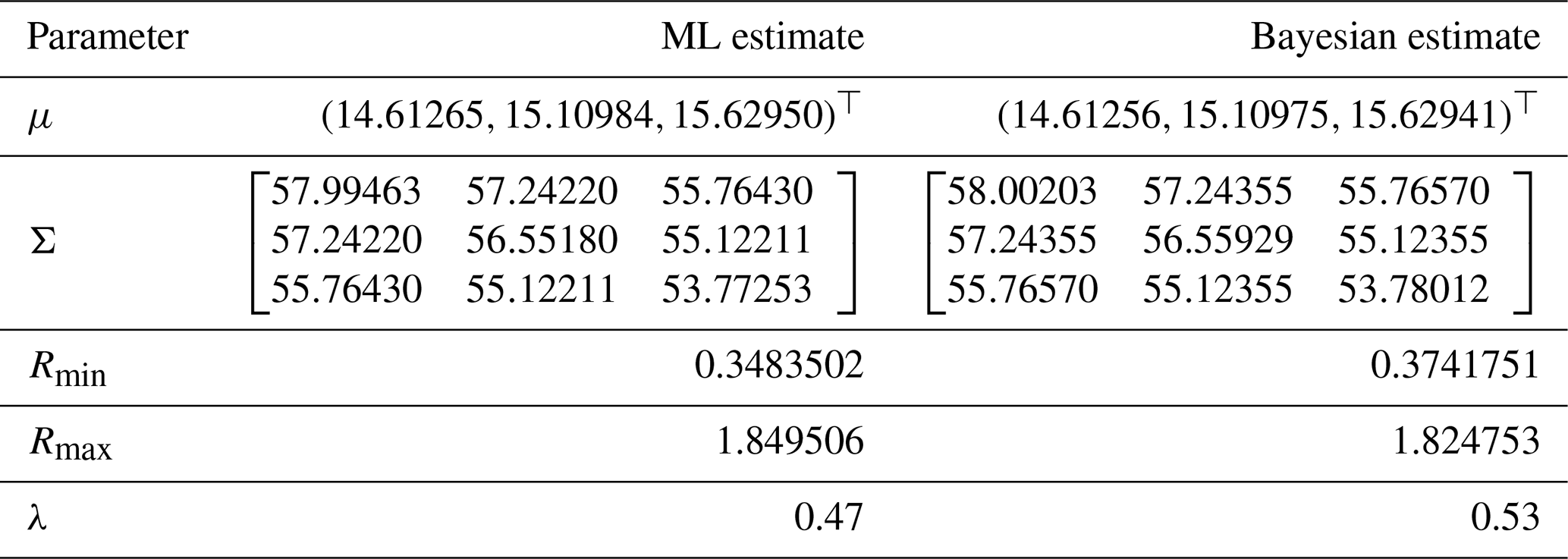
The total number of monthly observations, n=165, spans from January 2000 to September 2013, resulting in 165 vectors of symbolic data, each representing monthly summary statistics of average temperatures. The hyperparameters for the Bayesian estimation are as follows: κ=0.001, ${\mathit{\mu }}_{\mathrm{0}}=(\mathrm{0},\mathrm{0},\mathrm{0}{)}^{\top }$, ν₀=3, ${\mathrm{\Psi }}_{\mathrm{0}}=I_{\mathrm{3}\times \mathrm{3}}$, a=0.3, b=0.4, c=1.8, and d=2.0.

Table 4 summarizes the results from both the ML and Bayesian estimations.

Table 4 Comparison of ML and Bayesian estimates for monthly average temperatures in the United States.

5.1.2 Density estimators

In this section, we explore three methods for estimating predictive densities: posterior predictive density, the ML method, and the Bayesian plugin method. These methods provide different approaches to predicting future monthly average temperatures in the United States.

The ML and Bayesian plugin density estimators, using the ML and Bayesian estimators for μ, Σ, and λ from Table 4, can be obtained easily and are denoted by $p({\mathbf{Q}}^{*}\mid \widehat{\mathit{\mu }},\widehat{\mathbf{\Sigma }},\widehat{\mathit{\lambda }})$ and $p({\mathbf{Q}}^{*}\mid {\widehat{\mathit{\mu }}}_{\text{Bayes}},{\widehat{\mathbf{\Sigma }}}_{\text{Bayes}},{\widehat{\mathit{\lambda }}}_{\text{Bayes}})$, respectively. On the other hand, the posterior predictive density for a new random variable Q^* given the observations ${\mathbf{Q}}_{\mathrm{1}},\mathrm{\dots },{\mathbf{Q}}_n$ when λ is unknown is a mixture of multivariate Student's t distributions, as given in Eq. (26). If λ has already been estimated using ML or Bayesian methods, the posterior predictive density simplifies to a Student's t distribution as shown in Eq. (25).

Figure 3 Boxplots of summer average temperatures in European countries.

5.2 Analysis of summer average temperatures in European countries

In this subsection, we extend our analysis to examine summer average temperatures across various European countries, utilizing historical climate data that provide comprehensive temperature records dating back to the 18th century. The dataset includes average monthly temperature data measured from numerous weather stations situated in major cities across Europe, allowing for an in-depth analysis of long-term climate trends and variations.

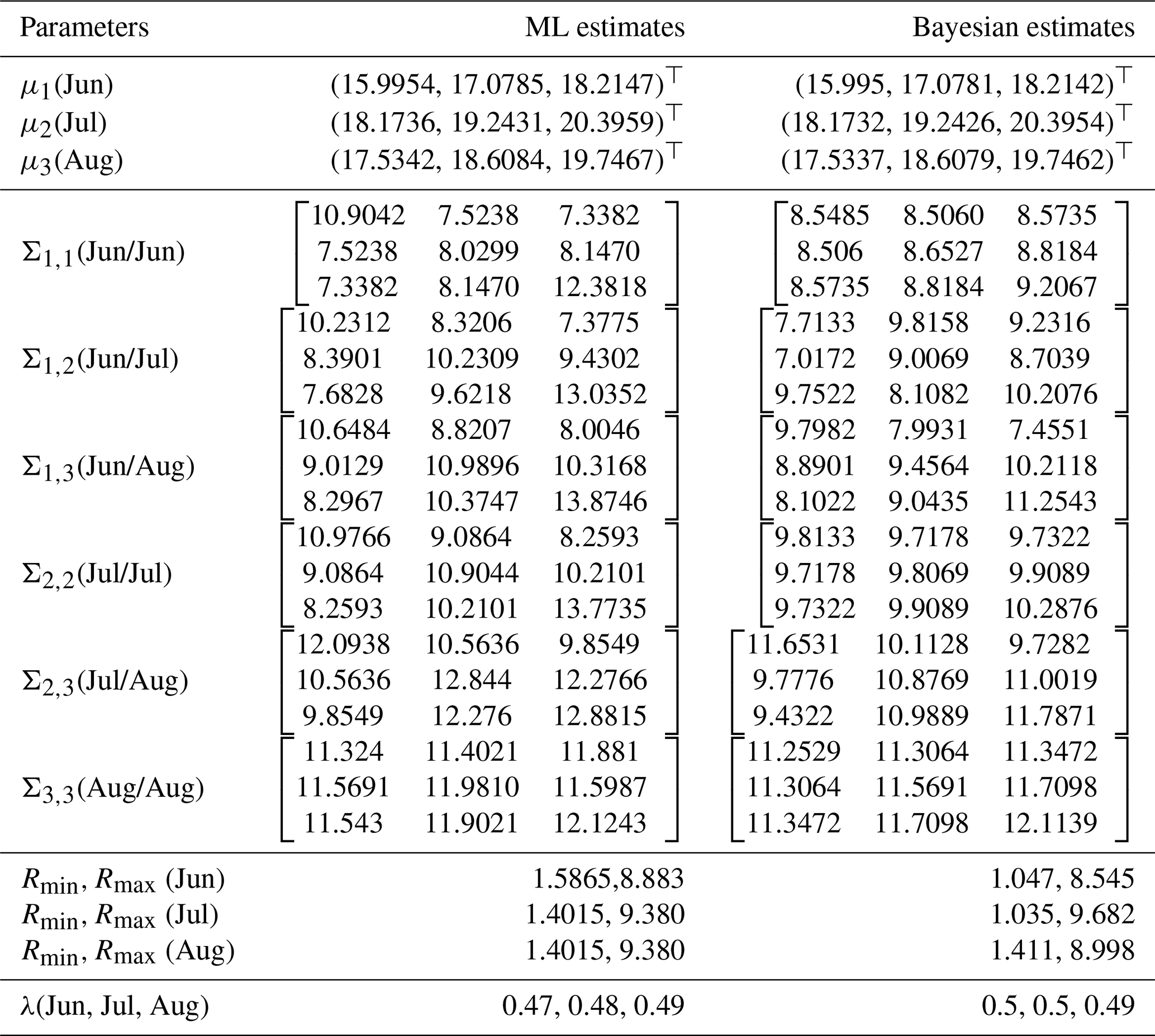
The analysis focuses on temperature records from 41 European countries, covering the three summer months June, July, and August. This extensive temporal and spatial coverage enables us to explore regional differences and similarities in temperature trends, contributing to a broader understanding of global climatic patterns.

Table 5 ML and Bayesian estimates for summer average temperatures in European countries.

The dataset was filtered to include only European countries, with the average temperatures for the summer months extracted for further analysis. Boxplots were then generated to visualize the distribution of average temperatures across countries during the summer season. Each boxplot represents the distribution of average temperatures for a specific country across the three summer months.

Figure 3 presents these boxplots, providing a clear illustration of the temperature variations and trends across Europe. This comparative study highlights the regional climatic patterns, offering valuable insights into the broader context of global climate change.

To further understand the differences between the ML and Bayesian approaches in estimating summer average temperatures in European countries, we present a comparative analysis of the estimators for the mean vectors and covariance matrices across the three summer months: June, July, and August. Table 5 summarizes the results.

The table above presents a side-by-side comparison of the ML and Bayesian estimators for the mean vectors and covariance matrices of summer average temperatures in European countries. The results show a close alignment between the ML and Bayesian estimates for the mean vectors across the three summer months. However, the covariance matrices exhibit some differences, particularly in the off-diagonal elements, which suggest variations in how each method captures the relationships between temperature readings across different months.

For instance, the Bayesian estimators tend to produce more consistent estimates across the covariance matrices, potentially reflecting the smoothing effect of prior information. The parameters R_min and R_max for each month also indicate that the range of temperature variations is slightly narrower in the Bayesian framework, further highlighting the influence of the priors.

6 Discussion

In this article, we have introduced a novel method for estimating the parameters of boxplot-valued random variables from both Bayesian and frequentist perspectives. Working with boxplot-valued random variables enables us to efficiently summarize large datasets, as boxplots concisely represent extensive amounts of information. Our method offers a significant computational advantage, as we derived closed-form solutions for both ML and Bayesian estimators. These closed-form expressions allow for direct computation of parameter estimates without the need for iterative optimization procedures or Markov chain Monte Carlo (MCMC)-type methods, which are commonly required in traditional Bayesian approaches. By avoiding these computationally intensive steps, our method reduces the overall complexity and computational load, making it particularly suitable for large datasets.

Additionally, we have explored the density estimation of future random boxplots, providing a comprehensive tool for investigating and forecasting these distributions. Our approach was evaluated through simulations and demonstrated its accuracy and computational efficiency when compared with existing methods. Furthermore, we applied the proposed techniques to real environmental data to illustrate their practical utility and effectiveness in real-world scenarios.

Boxplot-valued data analysis is particularly useful in contexts where data are collected in large volumes and need to be summarized effectively without losing significant information. By adopting both Bayesian and frequentist methods, we provide a comprehensive framework that leverages the strengths of each approach. The Bayesian methods offer a probabilistic interpretation and incorporate prior information, which is valuable when data are scarce or expensive to obtain. On the other hand, the frequentist methods provide consistency and robustness when large amounts of data are available.

Furthermore, our study on the density estimation of future random boxplots enhances predictive modeling capabilities, which is crucial for applications such as environmental monitoring and climate forecasting. By accurately estimating the distribution of future data, decision-makers can make more informed predictions and plans.

Through extensive simulations, we validated the performance of our proposed methods, showcasing their accuracy and reliability. The application to real environmental data further underscores the practical relevance and adaptability of our techniques. Moreover, although the multivariate normal model theoretically allows for the possibility of overlapping quartiles, our empirical studies – including both simulations and real-world applications – consistently resulted in ordered quartiles ($q_{\mathrm{1}i}\le m_i\le q_{\mathrm{3}i}$). This empirical consistency indicates that, within the context of our data and analysis, the model effectively preserves the natural ordering of quartiles, thereby mitigating the theoretical limitation in practical scenarios. Overall, this work contributes to the growing field of symbolic data analysis by offering efficient and effective tools for handling boxplot-valued data, thereby broadening the scope and applicability of statistical methodologies in various domains.