Machine-learning-based probabilistic forecasting of solar irradiance in Chile

By the end of 2023, renewable sources covered 63.4 % of the total electric-power demand of Chile, and, in line with the global trend, photovoltaic (PV) power showed the most dynamic increase. Although Chile's Atacama Desert is considered to be the sunniest place on Earth, PV power production, even in this area, can be highly volatile. Successful integration of PV energy into the country's power grid requires accurate short-term PV power forecasts, which can be obtained from predictions of solar irradiance and related weather quantities. Nowadays, in weather forecasting, the state-of-the-art approach is the use of ensemble forecasts based on multiple runs of numerical weather prediction models. However, ensemble forecasts still tend to be uncalibrated or biased, thus requiring some form of post-processing. The present work investigates probabilistic forecasts of solar irradiance for regions III and IV in Chile. For this reason, eight-member short-term ensemble forecasts of solar irradiance for the calendar year 2021 are generated using the Weather Research and Forecasting (WRF) model; these are then calibrated using the benchmark ensemble model output statistics (EMOS) method based on a censored Gaussian law and its machine-learning-based distributional regression network (DRN) counterpart. Furthermore, we also propose a neural-network-based post-processing method, resulting in improved eight-member ensemble predictions. All forecasts are evaluated against station observations for 30 locations in the study area, and the skill of post-processed predictions is compared to the raw WRF ensemble. Our case study confirms that all studied post-processing methods substantially improve both the calibration of probabilistic forecasts and the accuracy of point forecasts. Among the methods tested, the corrected ensemble exhibits the best overall performance. Additionally, the DRN model generally outperforms the corresponding EMOS approach.

1 Introduction

According to the latest report of the International Renewable Energy Agency (IRENA, 2024), the largest ever increase in renewable-power capacity was observed in 2023, nearly 75 % of which was newly installed solar energy. As a result, by the end of 2023, the renewable-energy share had reached 43 % of the global installed power capacity, and this ratio was even higher in South America (71.4 %). In particular, renewable sources covered 63.4 % of the total electric-power demand of Chile, 39.7 % of which came from photovoltaic (PV) energy. In line with the global trend, with the addition of 1949 MW, in 2023, PV power accounted for the most substantial increase of 30.4 %.

Although Chile’s Atacama Desert is considered to be the sunniest place on Earth, with the highest long-term solar irradiance (Rondanelli et al., 2015), PV power production can be highly volatile, which raises a strong demand for accurate PV power forecasts from power grid operators. A standard approach to PV power forecasting is to consider global horizontal irradiance (GHI) forecasts (and possibly forecasts of other weather variables) and to convert them into PV power with the help of a model chain; see, for example, Mayer and Yang (2022) or Horat et al. (2025). In the present study, we concentrate on solar irradiance predictions as they are highly correlated with the PV model chain outputs.

Traditionally, solar irradiance forecasts are obtained as outputs of numerical weather prediction (NWP) models, which describe the behaviour of the atmosphere with the help of partial differential equations. The state-of-the-art approach is to run these models simultaneously with various initial conditions and/or parameterizations, resulting in a probabilistic prediction as part of an ensemble forecast (Bauer et al., 2015; Buizza, 2018a). Nowadays, all major weather centres operate their own ensemble prediction systems (EPSs); one of the most prominent is the Integrated Forecast System (IFS) of the European Centre for Medium-Range Weather Forecasts (ECMWF), providing 51-member medium-range ensemble forecasts at 9 km resolution and 101-member extended-range forecasts at 32 km resolution (ECMWF, 2024). Nevertheless, in the last few years, NWP models gained strong competitors in the form of machine-learning-based, fully data-driven forecasts such as Pangu-Weather (Bi et al., 2023) or the more recent ECMWF Artificial Intelligence Forecasting System (AIFS; Lang et al., 2024), which was the first to issue AI-based ensemble predictions, followed by GenCast of Google DeepMind (Price et al., 2025).

Despite the efforts devoted to improving the EPSs, ensemble forecasts might exhibit deficiencies such as bias or lack of calibration, thus requiring some form of statistical post-processing (Buizza, 2018b). In the last decades, many post-processing methods have been suggested for a wide spectrum of weather variables; for an overview, see, for example, Vannitsem et al. (2021) or Schulz and Lerch (2022). Among these parametric approaches are the ensemble model output statistics method (EMOS; Gneiting et al., 2005) and the distributional regression network approach (DRN; Rasp and Lerch, 2018), which provide full predictive distributions in the form of a single parametric law. In the EMOS method, the parameters of the predictive distribution depend on the forecast ensemble via appropriate link functions, whereas, in the DRN approach, one trains a neural network, which connects the ensemble forecasts and possible other covariates to the distributional parameters. EMOS and DRN models for different weather quantities usually differ in terms of the parametric family describing the predictive distribution, and the EMOS link functions and the architectures of the DRN networks might also vary. Nonparametric methods include quantile regression, providing the predictive distribution in terms of its quantiles using either statistical tools (Friederichs and Hense, 2007; Bremnes, 2019) or machine learning techniques (Taillardat et al., 2016; Bremnes, 2020), and methods that directly improve the raw ensemble predictions, such as quantile mapping (Hamill and Scheuerer, 2018) or member-by-member post-processing (Van Schaeybroeck and Vannitsem, 2015).

To calibrate solar irradiance ensemble forecasts, Schulz et al. (2021) suggest EMOS models based on censored logistic and censored normal (CN0) distributions, while Baran and Baran (2024) and Horat et al. (2025) propose DRN counterparts of the latter. Furthermore, La Salle et al. (2020) compare linear quantile regression and the analogue ensemble technique to EMOS models utilizing truncated normal and truncated generalized extreme-value distributions. Bakker et al. (2019) consider quantile regression, quantile regression neural networks, random forests, and gradient-boosting decision trees, while Song et al. (2024) propose a non-crossing quantile regression neural network. According to the classification of Yang and van der Meer (2021), all the post-processing methods mentioned above can be considered to be probabilistic-to-probabilistic (P2P) approaches; see also Yang and Kleissl (2024, Sect. 8.6).

The present work investigates probabilistic forecasts of solar irradiance for regions III and IV in Chile, covering an area with the second-largest PV power potential after the Atacama Desert (Molina et al., 2017). For this reason, eight-member ensemble forecasts of solar irradiance for the calendar year 2021 are generated using the Weather Research and Forecasting (WRF) model (Skamarock et al., 2019); these are then calibrated using the benchmark CN0 EMOS model and its DRN counterpart. Furthermore, we also propose a neural-network-based post-processing method, resulting in improved eight-member ensemble predictions. All forecasts are evaluated against station observations for 30 locations in the study area, and, in a detailed case study, the skill of post-processed predictions is compared to the raw WRF ensemble. To the best of the authors' knowledge, no studies have been published yet that address the post-processing of solar irradiance ensemble forecasts for this part of the world. Thus, the main contributions of this work can be summarized in the following way.

• This paper provides a detailed analysis of the forecast skill of WRF probabilistic predictions of solar irradiance for two Chilean regions that are particularly important from the point of view of PV power production.

• This paper investigates the skill of state-of-the-art parametric post-processing methods.

• We also develop a machine-learning-based method for generating improved irradiance ensemble forecasts and assess its predictive performance.

The paper is organized as follows. The description of the WRF model configurations and the observed data and a preliminary assessment of the performance of WRF forecasts are given in Sect. 2. Section 3 introduces the applied post-processing methods, the approaches to training-data selection for modelling, and the considered forecast evaluation tools. The results of our case study are reported in Sect. 4, and the paper concludes with a summary and discussion in Sect. 5.

2 Data

2.1 WRF model configuration and ensemble members

The Advanced Research module of the Weather Research and Forecasting (WRF) model, version 4.4.2 (Skamarock et al., 2019), was used in this study. We consider eight-member ensemble forecasts for solar irradiance (downward shortwave flux given in W m⁻²) for the calendar year 2021 as generated by the model. All forecasts are initialized at 00:00 UTC with a 1 h temporal resolution and a forecast horizon of 48 h. The eight simulations were configured with two nested domains, as depicted in Fig. 1a, with 9 km (d01) and 3 km (d02) horizontal resolutions, 36 vertical levels at variable resolutions, and enhanced density near the surface and the tropopause. We will show only the results for the smallest domain (d02) with the highest resolution (3 km), provided separately in Fig. 1b. This domain includes regions III and IV of Chile, covering several coastal and interior towns and cities to the west and part of the Andes Cordillera to the east. Forecasts from the Global Forecast System (GFS) model at 0.25°×0.25° horizontal resolution provided the initial and boundary conditions for the WRF model regional forecasts every 3 h. The WRF simulations employed land use data based on the Moderate Resolution Imaging Spectroradiometer (MODIS) at 15 arcsec (approximately 0.4 km in horizontal resolution). We also set a two-way interaction, which allows the inner domain to provide feedback to its parent domain.

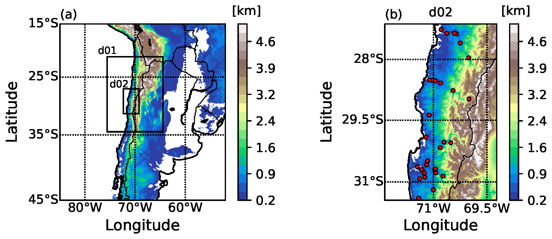
Figure 1 (a) The two WRF nested-domain configurations (d01 and d02) used for each simulation and the region's topography (shaded colours). (b) Zoomed-in image of domain d02, showing the location of the 30 observation stations (red circles).

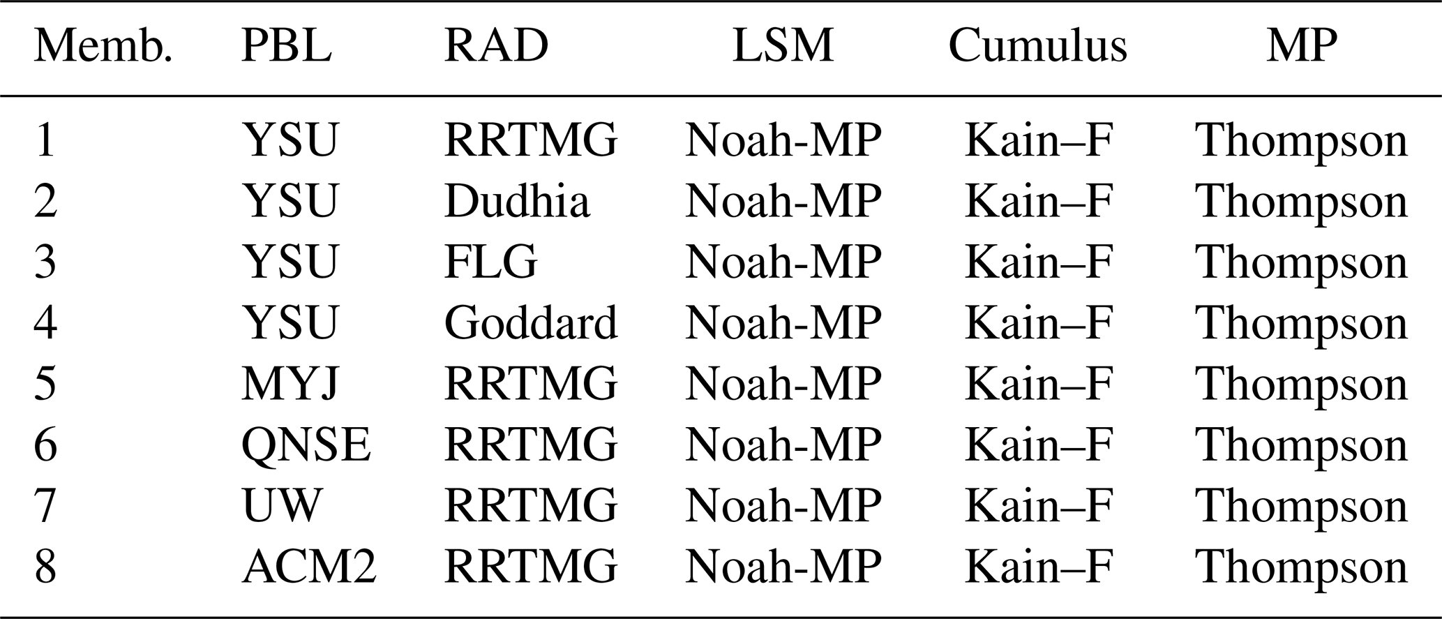
The eight simulations used the Noah-MP land surface model (Niu et al., 2011; Yang et al., 2011) to parameterize the surface–atmosphere interaction in all domains. The Noah-MP scheme forecasts the soil temperature and moisture and provides fractional snow cover and frozen-soil physics. Convective processes in all domains were calculated with the Kain–Fritsch scheme (Kain–F; Kain, 2004), while the Thompson double-moment scheme (Thompson et al., 2008) was used for microphysics. The eight-member simulations differ in terms of the employed radiation and planetary boundary layer (PBL) scheme. Four radiation and five PBL schemes were combined to form the eight-member simulations, whose descriptions are displayed in Table 1. The Yonsei University model (YSU; Hong et al., 2006), the Mellor–Yamada–Janjić model (MYJ; Janjić, 1994), the quasi-normal-scale elimination model (QNSE; Sukoriansky et al., 2005), the University of Washington model (UW; Bretherton and Park, 2009), and the asymmetric convective model (ACM2; Pleim, 2007) were used to calculate the PBL processes, whereas the rapid radiative transfer model (RRTMG; Iacono et al., 2005), the Dudhia model (Dudhia, 1989), the Fu–Liou–Gu model (FLG; Gu et al., 2011), and the new Goddard scheme (Chou et al., 1999, 2001) were used to parameterize the longwave and shortwave radiation processes. Note that one could have considered more combinations of PBL and radiation schemes, resulting in more ensemble members. However, on the one hand, we had limited computational resources, which posed constraints on both the ensemble size and the horizontal resolution. On the other hand, the current study is part of a broader research project dealing with the calibration of renewable-energy-related quantities (solar irradiance, wind speed, precipitation accumulation) in Chile, and we wanted to ensure comparability with our earlier results on post-processing eight-member WRF temperature (Díaz et al., 2020) and wind speed (Díaz et al., 2021) predictions. The relatively small ensemble size might affect the variability of the raw WRF forecasts; nonetheless, it does not affect the choice of the possible post-processing methods.

Table 1 Description of radiation (RAD), planetary boundary layer (PBL), land surface model (LSM), cumulus, and microphysics (MP) parameterizations used for each of the eight WRF ensemble members.

2.2 Solar irradiance observations

Solar irradiance observations (given in W m⁻²) are provided by the Chilean national weather service (DMC, an abbreviation for the Spanish name). We consider data from 30 stations in the Atacama and Coquimbo regions, between the coast and the Andes Cordillera. Table 2 describes each station's name and location (latitude, longitude, altitude), and Fig. 1b shows their spatial distribution over the study region. The observations with hourly temporal resolution were downloaded from the website: https://climatologia.meteochile.gob.cl/ (last access: 1 March 2025).

Table 2 The name, longitude, latitude, altitude, and region of 30 irradiance observation stations used in this study.

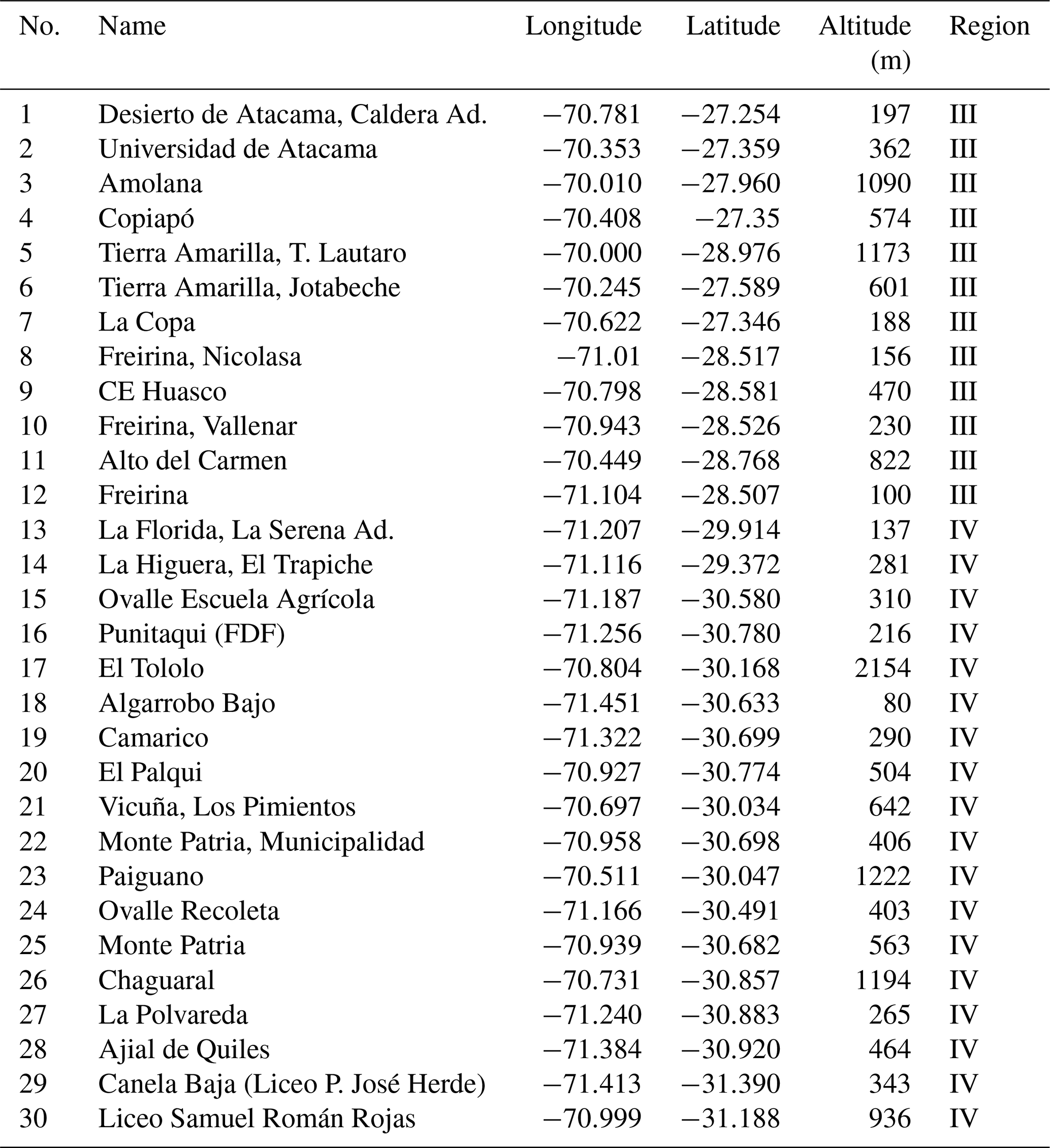
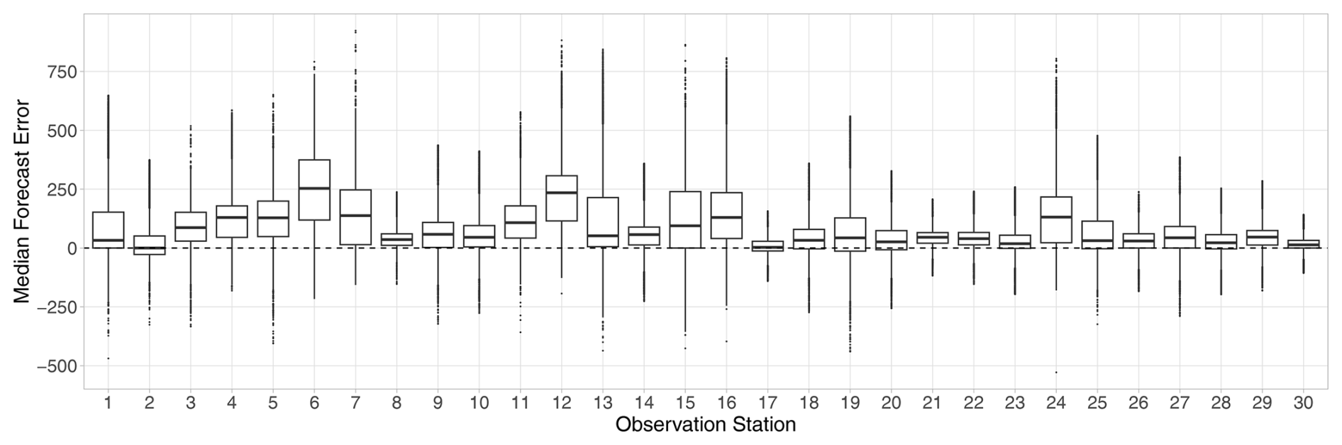
Figure 2 Median forecast error (W m⁻²) of the WRF ensemble at the observation stations listed in Table 2 for all dates and lead times of 12–24 h and 36–48 h.

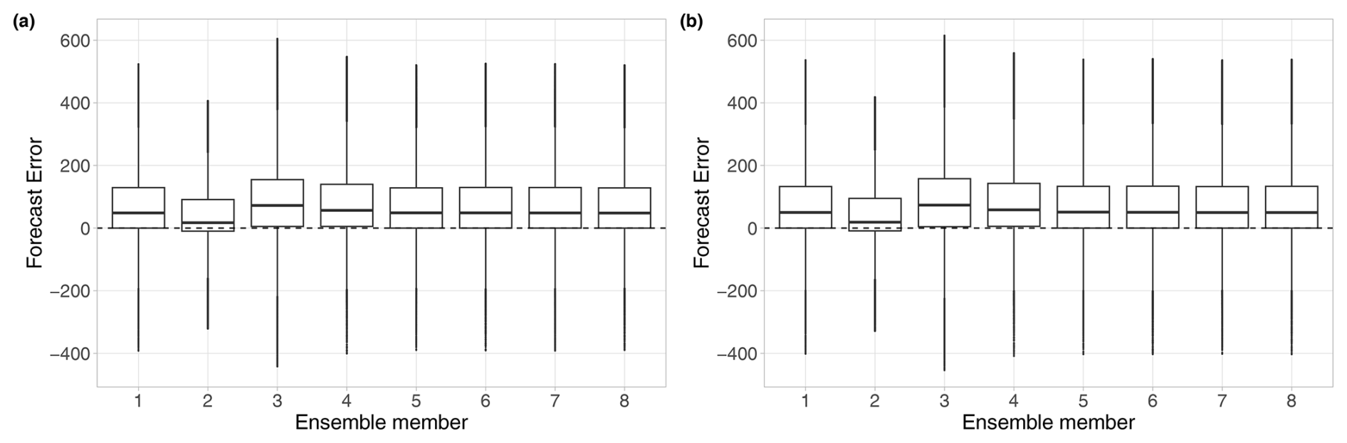
Figure 3 Forecast error (W m⁻²) of the individual ensemble members for all dates and locations for lead times of (a) 12–24 h and (b) 36–48 h.

Figure 4 Forecast error (W m⁻²) of the ensemble median for all dates and locations as functions of the lead time.

2.3 Forecast skill of the WRF ensemble

The matching of the WRF ensemble predictions with observations at the monitoring stations listed in Table 2 is performed by extracting forecasts for the nearest grid points from the WRF domain d02. As depicted in Fig. 1b, the topography of this region is rather complex; the station altitudes range from 80 to 2154 m, and the differences in terms of station elevation have an impact on the forecast performance. Figure 2 shows the boxplots of the median forecast error of the WRF ensemble (median deviation of the eight individual ensemble members from the verifying observation, that is, the median bias of the WRF members) at the various observation stations for the whole calendar year 2021 for lead times corresponding to the period between 12:00 and 00:00 UTC, when positive irradiance is likely to be observed. Raw WRF forecasts systematically overestimate the actual irradiance, and both the magnitude of the bias and the spread of the median forecast error strongly depend on the location. However, in contrast to Díaz et al. (2020), where the station altitude played a key role in the capability of WRF temperature forecasts, here, despite the WRF irradiance ensemble performing the best at the highest station (no. 17; El Tololo), one cannot find a clear connection between the elevation and the forecast skill. The same positive bias can be observed in Fig. 3, displaying the boxplots of the forecast error of the individual ensemble members for all dates and locations, treating shorter (12–24 h) and longer (36–48 h) lead times separately. Although longer forecast horizons result in slightly larger forecast errors, Fig. 3a and b convey the same message. Ensemble member 2 substantially outperforms the other seven members by exhibiting the smallest bias; the largest error corresponds to member 3, followed by member 4, whereas the performance of members 1 and 5–6 is fairly similar. Finally, the boxplots of the diurnal evolution of the forecast error of the ensemble median depicted in Fig. 4 indicate that the positive bias is also systematic along the forecast horizons of 12–24 h and 36–48 h, when positive irradiance is likely to be observed, and the largest errors correspond to 15:00 and 16:00 UTC, when the solar irradiance reaches its peak.

3 Post-processing and forecast evaluation methods

As mentioned in the Introduction, we consider two different parametric methods for post-processing WRF solar irradiance ensemble forecasts. The key step in parametric modelling is the choice of the predictive distribution. Addressing non-negativity of solar irradiance, several parametric models utilize distributions left truncated from below at zero; see, for example, La Salle et al. (2020) or Yang (2020). However, such models require the specification of times of day with positive irradiance, whose periods depend strongly on the location and season. This deficiency can be solved by considering laws that assign a positive mass to the event of zero irradiance as such a distribution can handle even the night hours, when both predicted and observed irradiance are zero. A popular choice is to left censor a suitable distribution at zero, which proved to be successful a successful approach, e.g. in modelling precipitation accumulation (Scheuerer, 2014; Baran and Nemoda, 2016). Here, we utilize the censored normal EMOS approach of Schulz et al. (2021), considered to be a benchmark method, and the corresponding DRN model investigated by Baran and Baran (2024) and Horat et al. (2025). Parametric models based on this particular predictive distribution demonstrated excellent skill for various ensemble forecasts covering different geographical areas.

Beyond parametric modelling, we also suggest a neural-network-based distribution-free ensemble correction technique, where the output is a calibrated forecast ensemble. Although, in this post-processing approach, there is no restriction on the number of generated corrected forecasts, for the sake of fair comparability, we consider the ensemble size of eight of the raw WRF ensembles.

Compared to the EMOS and DRN models, the aforementioned method lacks the advantage of providing a full predictive distribution; however, similarly to the nonparametric post-processing techniques, it allows more flexible modelling, and the output can be interpreted in the same way as the raw ensemble forecast.

In what follows, let f₁, f₂, …, f₈ denote the eight-member WRF irradiance forecast of a given forecast horizon for a given location and time, and let $\stackrel{\mathrm{‾}}{f}$ and S² denote the corresponding ensemble mean and variance, respectively.

3.1 EMOS model for solar irradiance

Let $G\left(x\right|\mathit{\mu },\mathit{\sigma })$ denote the cumulative distribution function (CDF) of a Gaussian distribution with mean μ and standard deviation σ>0:

$$G\left(x\right|\mathit{\mu },\mathit{\sigma }):=\mathrm{\Phi }\left({\displaystyle \frac{x-\mathit{\mu }}{\mathit{\sigma }}}\right),x\in \mathbb{R},$$

with Φ denoting the CDF of a standard normal law. Then the CDF of a normal distribution with location μ and scale σ left censored at zero (CN0) equals

$$\begin{array}{}\text{(1)}& G_{\mathrm{0}}^c\left(x\right|\mathit{\mu },\mathit{\sigma }):=\left\{\begin{array}{ll}G\left(x\right|\mathit{\mu },\mathit{\sigma }),& x\ge \mathrm{0},\\ \mathrm{0},& x<\mathrm{0}\end{array}\right..\end{array}$$

This distribution assigns mass $G_{\mathrm{0}}^c\left(\mathrm{0}\right|\mathit{\mu },\mathit{\sigma })$ to the origin and has a mean of

$$\mathit{\kappa }=\mathit{\mu }\mathrm{\Phi }(\mathit{\mu }/\mathit{\sigma })+\mathit{\sigma }\mathit{\phi }(\mathit{\mu }/\mathit{\sigma }),$$

where φ denotes the standard normal probability density function (PDF). Following Schulz et al. (2021) and Baran and Baran (2024), the ensemble members are connected to the parameters of the CN0 distribution via equations (link functions):

$$\mathit{\mu }={\mathit{\gamma }}_{\mathrm{0}}+{\mathit{\gamma }}_{\mathrm{1}}\stackrel{\mathrm{‾}}{f}+{\mathit{\gamma }}_{\mathrm{2}}{p}_{\mathrm{0}}\mathrm{and}\mathit{\sigma }=\exp \left({\mathit{\delta }}_{\mathrm{0}}+{\mathit{\delta }}_{\mathrm{1}}\log S\right),$$

where p₀ is the proportion of WRF ensemble members predicting zero irradiance; that is,

$$p_{\mathrm{0}}:={\displaystyle \frac{\mathrm{1}}{\mathrm{8}}}\sum _{k=\mathrm{1}}^{\mathrm{8}}{\mathbb{I}}_{\left\{f_k=\mathrm{0}\right\}},$$

with 𝕀_H denoting the indicator function of a set H. Model parameters γ₀, γ₁, γ₂, δ₀, and δ₁∈ℝ are estimated following the optimum score principle of Gneiting and Raftery (2007) that is obtained by minimizing the mean value of a proper scoring rule (in our case, the continuous ranked probability score (CRPS) defined by Eq. (2) in Sect. 3.5) over appropriate training data comprising past forecast–observation pairs. This general approach is the most standard in parametric ensemble post-processing, where replacing the CRPS with the ignorance score, defined as the negative logarithm of the predictive PDF evaluated for the corresponding observation (see, for example, Wilks, 2019, Sect. 9.5.3), results in the conventional maximum-likelihood estimates.

3.2 DRN model for solar irradiance

Distributional regression networks (DRNs), first employed by Rasp and Lerch (2018) for calibrating temperature ensemble forecasts, represent an advanced class of machine-learning-based post-processing models. Similarly to the EMOS approach, they extend traditional regression techniques by predicting parameters of the forecast distribution belonging to a given family, in our case, the location μ and scale σ of the CN0 distribution specified by the CDF (Eq. 1). The DRN approach enhances the statistical calibration of ensemble forecasts, providing a more comprehensive understanding of prediction uncertainty. DRNs typically leverage predictor variables, such as NWP quantities and station characteristics, to inform their predictions. Additionally, station embeddings enable the network to recognize location-specific information, capturing unique features and patterns relevant to individual stations.

DRNs are often implemented using a multilayer perceptron (MLP; Goodfellow et al., 2016) architecture, which improves their ability to capture complex relationships between the NWP forecasts and other covariates and the distributional parameters to be predicted. The feed-forward structure of the network allows input features to pass through multiple hidden layers, where neurons apply weighted transformations and activation functions to the input signals. Activation functions such as ReLU (rectified linear unit), sigmoid, or tanh introduce non-linearity, enabling the model to learn intricate patterns and relationships in the data. Similarly to EMOS modelling, the weights of the MLP neural networks connecting the input covariates with the distributional parameters μ and σ are estimated by minimizing the mean CRPS of the CN0 predictive distributions over the training data, optimizing probabilistic forecasts to align with observed outcomes. Note that, building upon the work of Rasp and Lerch (2018), which focused on fully connected networks such as MLP, recently, convolutional layers have also gained popularity within DRNs (Veldkamp et al., 2021; Li et al., 2022). These layers leverage local patterns and spatial hierarchies in the data, further enhancing the model's ability to capture complex relationships. However, in this study, we keep the traditional MLP architecture, consisting of an input layer with as many neurons as the number of input covariates, a few hidden layers (shallow network), and an output layer with two neurons corresponding to the distributional parameters. Further details regarding the applied MLP network can be found in Sect. 3.6.

To further enhance model performance and to prevent overfitting, early stopping is often employed as a regularization technique during training. By monitoring performance based on a validation dataset, training halts when improvements cease, ensuring the model retains its generalization capabilities. This approach not only optimizes the training process but also contributes to more robust predictions.

3.3 Machine-learning-based forecast improvement

In addition to constructing predictive distributions, another possible alternative is statistical post-processing using machine learning models that generate improved ensemble forecasts. For this purpose, similarly to the DRN model described in Sect. 3.2, we use a neural network based on the MLP architecture; however, here, the number of neurons in the output layer equals the number of ensemble members to be generated. The other principal difference is the implementation of the loss function. Due to the nature of the output, here, we apply the ensemble CRPS given by Eq. (3) (see Sect. 3.5), with the constraint that the predicted solar irradiance forecasts can only be non-negative. This post-processing method is flexible as it is distribution-free, and the number of ensemble members to be generated is up to the user, provided enough training data are available. However, to ensure direct comparability with the WRF forecasts, we create an eight-member prediction, referred to as the corrected ensemble, for each verification day, location, and forecast horizon.

3.4 Training-data selection

The efficiency of all post-processing methods, including the ones described in Sect. 3.1–3.3, strongly depends on the spatial and temporal decomposition of the training data.

From the point of view of temporal selection, a popular approach is using a sliding window, where the model for a given date is trained using forecast–observation pairs from the preceding n calendar days. This simple method, also utilized in our study, allows for a quick adaptation to seasonal variations or model changes; nevertheless, larger time shifts, such as monthly, seasonal, or yearly windows, might also be beneficial (see, for example, Jobst et al., 2023). Alternatively, one can consider a fixed, very long training period, a popular approach in machine-learning-based post-processing methods requiring a large amount of training data (see, for example, Schulz and Lerch, 2022; Horat et al., 2025). For a systematic comparison of time-adaptive model training schemes, we refer the reader to Lang et al. (2020).

Regarding the spatial composition of training data, the traditional approaches are local and regional (global) modelling (Thorarinsdottir and Gneiting, 2010). Local models are based on past forecast–observation pairs for the actual location under consideration, whereas the regional approach utilizes historical data of all studied stations. In general, local models outperform their regional counterparts, provided one has enough location-specific training data to avoid numerical issues during the calibration process. The regional approach, resulting in a single set of EMOS parameters or neural network weights for the whole ensemble domain, is more suitable if only short training periods are allowed; however, it might hardly handle large and heterogeneous areas. To combine the advantageous properties of the above two approaches to spatial selection, Lerch and Baran (2017) suggested a novel clustering-based semi-local method which appeared to be successful for several different weather variables and ensemble domains; see, for example, Baran et al. (2020), Szabó et al. (2023), or Baran and Lakatos (2024). For a given date of the verification period, a feature vector is assigned to each observation station, representing the station climatology and the forecast error of the ensemble mean during the training period. Based on these feature vectors, the stations are then grouped into clusters using k-means clustering (see, for example, Wilks, 2019, Sect. 16.3.1), and, within each cluster, regional modelling is performed. In the case of rolling training windows, the stations are regrouped dynamically for each particular training set.

3.5 Forecast verification

As mentioned, the parameters of the CN0 EMOS model described in Sect. 3.1 are estimated by minimizing the mean of a proper scoring rule over the training data. In particular, we consider the continuously ranked probability score (CRPS; Wilks, 2019, Sect. 9.5.1), which is probably the most popular proper verification score in atmospheric sciences. Given a probabilistic forecast expressed as a predictive CDF F and an observation x∈ℝ, the CRPS is defined as

$$\begin{array}{}\text{(2)}& \begin{array}{rl}\mathrm{CRPS}(F,x)& :=\underset{-\mathrm{\infty }}{\overset{\mathrm{\infty }}{\int }}{\left[F\left(y\right)-{\mathbb{I}}_{\mathit{\{}y\ge x\mathit{\}}}\right]}^{\mathrm{2}}\mathrm{d}y\\ & =E|X-x|-{\displaystyle \frac{\mathrm{1}}{\mathrm{2}}}E|X-X^{\prime }|,\end{array}\end{array}$$

where X and X^′ are independent random variables distributed according to F and with a finite first moment. The CRPS is a negatively oriented score (smaller values indicate better performance), and it simultaneously assesses both the calibration and the sharpness of a probabilistic forecast. Calibration means a statistical consistency between forecasts and observations, while sharpness refers to the concentration of the probabilistic forecasts. Furthermore, the expression of the CRPS on the right-hand side of Eq. (2) indicates that it can be expressed in the same unit as the observation. For the censored normal distribution considered in Sect. 3.1 and 3.2, the CRPS has a closed form (see, for example, Jordan et al., 2019), which allows for a computationally efficient numerical optimization, hence making it eligible to serve as a loss function in both EMOS and DRN modelling. For a forecast ensemble f₁, f₂, …, f_K, one should consider the empirical CDF ${\widehat{F}}_K$, resulting in the expression

$$\begin{array}{}\text{(3)}& \mathrm{CRPS}({\widehat{F}}_K,x)={\displaystyle \frac{\mathrm{1}}{K}}\sum _{k=\mathrm{1}}^K|f_k-x|-{\displaystyle \frac{\mathrm{1}}{\mathrm{2}{K}^{\mathrm{2}}}}\sum _{k=\mathrm{1}}^K\sum _{\mathrm{\ell }=\mathrm{1}}^K|f_k-f_{\mathrm{\ell }}|.\end{array}$$

See, for example, Krüger et al. (2021). The same definition applies to the corrected ensemble forecast produced by the approach described in Sect. 3.3 and to the calibrated samples generated from the EMOS or DRN predictive distributions. Note that the above formula differs slightly from the ensemble CRPS given in Wilks (2019, Sect. 9.7.3); however, in the R package scoringRules (Jordan et al., 2019), the expression of Eq. (3) is implemented.

In the case study of Sect. 4, the predictive performance of the competing probabilistic forecasts with a given forecast horizon is compared with the help of the mean CRPS over all forecast cases in the verification period. Furthermore, we also quantify the improvement in the mean CRPS of a probabilistic forecast F for a reference forecast F_ref using the continuous ranked probability skill score (CRPSS; see, for example, Gneiting and Raftery, 2007). This positively oriented quantity (the larger, the better) is defined as

$$\mathrm{CRPSS}:=\mathrm{1}-{\displaystyle \frac{{\stackrel{\mathrm{‾}}{\mathrm{CRPS}}}_F}{{\stackrel{\mathrm{‾}}{\mathrm{CRPS}}}_{F_{\mathrm{ref}}}}},$$

where ${\stackrel{\mathrm{‾}}{\mathrm{CRPS}}}_F$ and ${\stackrel{\mathrm{‾}}{\mathrm{CRPS}}}_{F_{\mathrm{ref}}}$ denote the mean CRPS corresponding to forecasts F and F_ref, respectively. In particular, in Sect. 4, for the reference prediction F_ref, we consider the raw WRF ensemble, while forecast F can be any of the post-processed predictions described in Sect. 3.1–3.3.

A separate assessment of the calibration and sharpness of predictive distributions can be obtained with the help of the coverage and average width of (1−α)100 %, $\mathit{\alpha }\in (\mathrm{0},\mathrm{1})$, central prediction intervals, respectively. By coverage, we mean the proportion of observations located between the $\mathit{\alpha }/\mathrm{2}$ and $\mathrm{1}-\mathit{\alpha }/\mathrm{2}$ quantiles of the predictive CDF, where properly calibrated forecasts result in values of around (1−α)100 % (see, for example, Gneiting and Raftery, 2007). For a k-member forecast ensemble, one usually considers the nominal coverage $(K-\mathrm{1})/(K+\mathrm{1})$100 % of the ensemble range (77.78 % for the eight-member WRF ensemble at hand), which is the probability of the rank of the observation for a calibrated prediction being greater than 1 and less than K+1. Choosing α to match this nominal coverage allows for a fair comparison of ensemble forecasts with forecasts provided as full predictive distributions.

A further plausible tool for evaluating the calibration of ensemble forecasts is the verification rank histogram (or Talagrand diagram). The Talagrand diagram displays the ranks of the verifying observation with respect to the corresponding ensemble prediction (Wilks, 2019, Sect. 9.7.1), which, for a calibrated k-member ensemble, should follow a discrete uniform law on the set {1, 2, …, K+1}. The shape of a rank histogram reflects the source of the lack of calibration: ∪- and ∩-shaped histograms refer to underdispersion and overdispersion, respectively, whereas biased forecasts result in triangular shapes. Furthermore, the deviation of the distribution of the verification ranks from the uniform law can be quantified with the help of the reliability index:

$$\mathrm{RI}:=\sum _{r=\mathrm{1}}^{K+\mathrm{1}}|{\mathit{\rho }}_r-{\displaystyle \frac{\mathrm{1}}{K+\mathrm{1}}}|,$$

where ρ_r denotes the relative frequency of rank r over all forecast cases in the verification period (Delle Monache et al., 2006). The continuous counterpart of the Talagrand diagram is the probability integral transform (PIT; Wilks, 2019, Sect. 9.7.1) histogram. The PIT is defined as the value of predictive CDF for the verifying observation, with possible randomization at the points of discontinuity. For a calibrated predictive distribution, PIT is standardly uniform, and the interpretation of the various deviations of the shapes of the PIT histograms from uniformity is similar to that for the Talagrand diagrams.

Furthermore, the accuracy of point forecasts such as the forecast median is evaluated with the mean absolute error (MAE) as the median minimizes this score (Gneiting, 2011).

Finally, the statistical significance in score differences is assessed by accompanying some skill scores and score differences by 95 % block bootstrap confidence intervals. We consider 2000 samples calculated using the stationary bootstrap scheme with block lengths following a geometric distribution with a mean proportional to the cube root of the length of the investigated time interval (Politis and Romano, 1994).

3.6 Modelling and implementation details

In the case of the EMOS modelling, all 48 forecast horizons are treated separately, and model parameters are estimated using a clustering-based semi-local approach. Similarly to Lerch and Baran (2017), we consider 24-D vectors, where half of the features comprise equidistant quantiles of the climatological CDF over the training period and the other half consist of equidistant quantiles of the empirical CDF of the forecast error of the ensemble mean. After testing several combinations of training-period length and number of clusters, an 85 d rolling window is chosen, and, in general, six clusters are formed (an average of 425 forecast–observation pairs for each estimation task), provided each cluster contains at least three observation stations. Otherwise, the number of clusters is reduced, which might result in regional modelling.

Machine-learning-based forecasts are estimated regionally, and a single MLP neural network is trained for all lead times. CN0 DRN models use 20 d rolling training windows, while corrected forecasts depend on forecast–observation pairs of the preceding 25 d. These training-period lengths are the results of detailed data analysis.

Through testing various hidden-layer configurations for the CN0 DRN approach, we identified an optimal MLP model with two hidden layers, each containing 255 neurons, and considered a batch size of 1200. To enhance numerical stability, we standardize input features and remove missing data. The model is trained with the “Adam” optimizer, a learning rate of 0.01, and the ReLU activation function. Input features include the ensemble mean $\stackrel{\mathrm{‾}}{f}$ and variance S², the proportion p₀ of zero-irradiance forecasts, station coordinates (latitude, longitude, altitude), and lead times. Feature importance was also assessed to evaluate each input's impact on model performance. The model output directly represents the parameters μ and σ of the CN0 predictive distribution, with only a squaring being applied to the scale parameter to ensure non-negativity.

The training is capped at 500 epochs, but an early stopping callback – using 20 % of the training data as a validation set – often enabled convergence at approximately 50 epochs for the first verification day, with fewer epochs being required on subsequent days. To address the randomness inherent in training, for each forecast case, we train the network 10 times, deriving final predictions by averaging the distribution parameters across these sessions.

Our detailed tests suggest that, when DRN input features are restricted to ensemble statistics used in EMOS modeling (i.e. the same set of explanatory variables), the DRN's performance generally aligns with that of EMOS. This indicates that, without additional input information beyond the functionals of the ensemble forecasts, DRNs may have limited capacity for performance gains over EMOS in terms of accuracy and calibration. Notably, including station location information contributed significantly to enhanced model performance, which aligns with the findings of Horat et al. (2025).

For the MLP network providing corrected forecasts, we also comprehensively tested different input features and hyperparameters, though optimal results were achieved with the same settings as for the CN0 DRN approach. Due to the increase in the neurons in the output layer from two to eight, the number of weights to be estimated increased from 67 832 to 69 368, which explains the 5 d increase in the training-period length. Furthermore, to ensure the non-negativity of the generated forecasts, we take the maximum of zero and the predicted value, which is consistent with the handling of negative predictions in the loss function. Finally, as before, to account for the stochastic nature of the model, 10 independent runs are performed for each forecast case. The generated forecasts are then sorted in ascending order, and the average is computed over the sorted values. Note that, without sorting, the averaging would decrease the spread of the obtained eight-member forecast, which would no longer bear the same distributional characteristics as the originally generated eight-member corrected ensembles.

From the point of view of computational costs, which are negligible compared with the cost of generating the raw ensemble forecasts, there are no substantial differences between the three investigated post-processing approaches. The two machine-learning-based methods have similar architectures and rely on the same type of training data to estimate the weights of a single neural network for all locations and lead times. In general, the optimization step in EMOS modelling is much faster than in network training; however, separate semi-local modelling for all lead times usually requires 6×48 individual EMOS models.

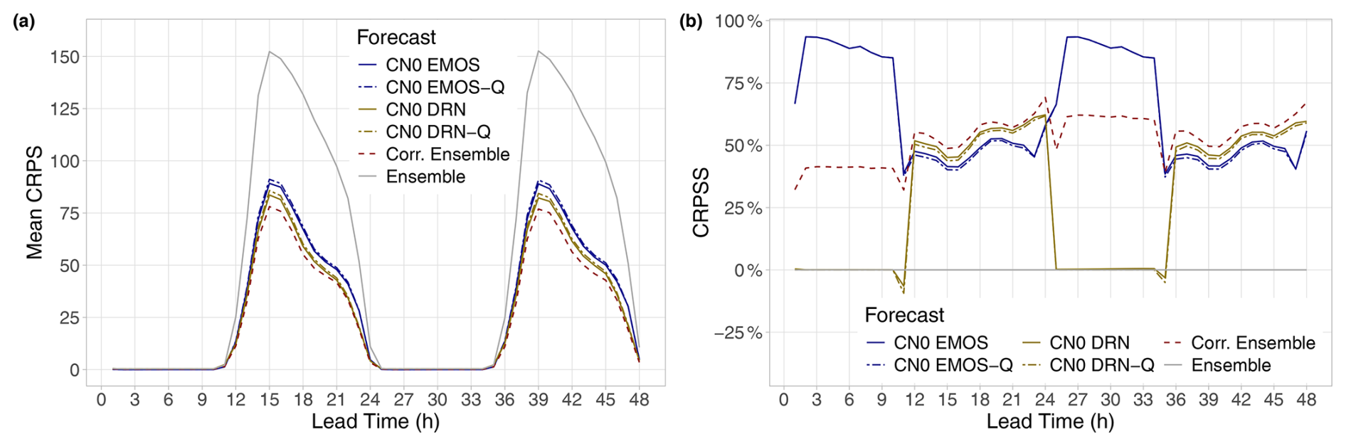
Figure 5 (a) Mean CRPS of raw and post-processed irradiance forecasts and (b) CRPSS of post-processed forecasts with respect to the raw WRF ensemble as functions of the lead time.

4 Results

In the following case study, the predictive performances of the CN0 EMOS and CN0 DRN approaches described in Sect. 3.1 and 3.2, respectively, are evaluated together with the machine-learning-based forecast improvement method presented in Sect. 3.3. To ensure a fair comparison of the latter with the EMOS and DRN models resulting in full predictive distributions, we also investigate the forecast skill of eight-member samples generated from the corresponding CN0 distributions, where one can consider their $\mathrm{1}/\mathrm{9}$, $\mathrm{2}/\mathrm{9}$, …, $\mathrm{8}/\mathrm{9}$ quantiles, simple random sampling, or stratified samples (Hu et al., 2016). As preliminary analysis reveals only minor differences in the skill of equidistant quantiles and stratified samples, both outperforming random sampling, here, we work with equidistant quantiles of CN0 EMOS and CN0 DRN predictive distributions. The corresponding forecasts are referred to as CN0 EMOS-Q and CN0 DRN-Q, respectively.

In the following analysis, the predictive performance of the competing post-processing methods is tested on forecast–observation pairs for the 9 months of 1 April–31 December 2021 (275 calendar days, right after the first 85 d training window used in EMOS modelling), and the raw WRF irradiance forecasts are used as a reference.

Figure 5a displays the mean CRPS of raw and post-processed WRF irradiance forecasts over all 30 locations and all 275 d in the verification period. Between 12:00 and 00:00 UTC (lead times of 12–24 h and 36–48 h), when positive irradiance is likely to be observed, all calibration methods outperform the raw ensemble by a wide margin. According to the CRPSS values of Fig. 5b, at this time of the day, the improvement with respect to the raw ensemble is around 50 % for all competing forecasts, and the ranking of the various methods is consistent for all forecast horizons. There are only minor differences in terms of skill between forecasts resulting in full predictive distributions (CN0 EMOS and CN0 DRN) and their sample counterparts (CN0 EMOS-Q and CN0 DRN-Q, respectively). The corrected ensemble results in the highest CRPSS, followed by the DRN and EMOS predictions. Note that, for 1–11 h and 25–35 h forecasts, the skill score values are irrelevant; they are just results of numerical issues.

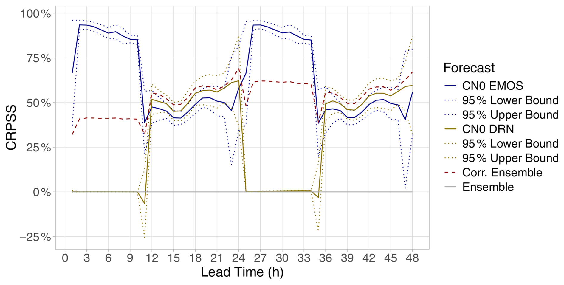
Figure 6 CRPSS with respect to the raw WRF ensemble of the CN0 EMOS and CN0 DRN models (together with 95 % confidence intervals) and the corrected ensemble as functions of the lead time.

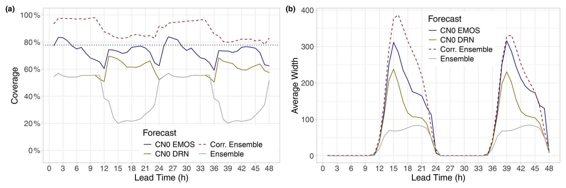
Figure 7 (a) Coverage and (b) average width of the nominal 77.78 % central prediction intervals of post-processed and raw irradiance forecasts as functions of the lead time. In (a), the ideal coverage is indicated by the horizontal dotted line.

The clear ranking of the various calibrated forecasts is also confirmed by Table 3, summarizing their mean CRPS as a proportion of the mean CRPS of the WRF ensemble for forecast cases where the observed irradiance is at least 7.5 W m⁻². Note that, from the point of view of PV energy production, only these cases are of any interest, and the threshold coincides with the one considered in Baran and Baran (2024) and suggested by the forecasters of the Hungarian Meteorological Service (HMS). One should also remark that the improvements in mean CRPS over the raw WRF ensemble provided in Table 3 are much higher than the gains due to CN0 EMOS and CN0 DRN post-processing of 11-member AROME-EPS forecasts (Jávorné Radnóczi et al., 2020) of the HMS, as reported by Baran and Baran (2024, Table 3). An even smaller advantage of the post-processed forecasts over the raw 40-member ICON-EPS predictions (Zängl et al., 2015) of the German Meteorological Service (DWD, Deutsche Wetterdienst) was observed by Schulz et al. (2021).

Table 3 Overall mean CRPS of post-processed irradiance forecasts as a proportion of the mean CRPS of the raw WRF ensemble for observed irradiance of no less than 7.5 W m⁻².

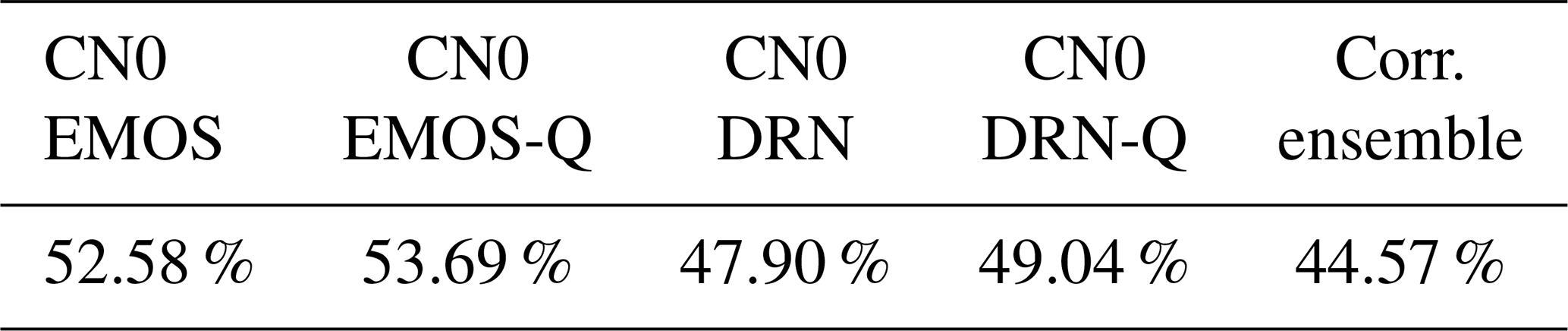
To investigate the statistical significance of the differences in terms of the mean CRPS, in Fig. 6, the corresponding 95 % confidence intervals are added to the CRPSS values of the CN0 EMOS and CN0 DRN approaches. For lead times corresponding to the 12:00–00:00 UTC interval, neither the difference between the corrected ensemble and the CN0 DRN nor the deviation of the CN0 EMOS and the CN0 DRN is significant; however, between 13–20 h and 37–44 h, the best-performing corrected ensemble significantly outperforms the worst-performing CN0 EMOS.

The improved calibration of post-processed forecasts can also be observed in Fig. 7a, displaying the coverage of the nominal 77.78 % central prediction intervals. To ensure comparability with the raw ensemble, for calibrated eight-member forecasts, we consider the coverage of the whole ensemble range. In the case of CN0 EMOS-Q and CN0 DRN-Q predictions based on equidistant quantiles of the corresponding predictive distributions, the ensemble ranges coincide with the 77.78 % central prediction intervals of the CN0 EMOS and CN0 DRN models, respectively, and so they are excluded from the analysis. At the hours of the highest solar irradiance (13:00–22:00 UTC), the coverage of the raw WRF forecasts is below 40 %, where post-processed forecasts result in coverage values much closer to the targeted 77.78 %. A possible ranking of the three investigated methods can be formed with the help of Table 4, providing the mean absolute deviation in coverage from the nominal level for 13:00–22:00 UTC observations. According to Fig. 7b, the improved coverage of calibrated forecasts is accompanied by wider prediction intervals; however, the CN0 EMOS prediction resulting in the best coverage values is considerably sharper than the second-best corrected ensemble.

Table 4 Mean absolute deviation in coverage from the nominal 77.78 % level over lead times corresponding to 13:00–22:00 UTC observations.

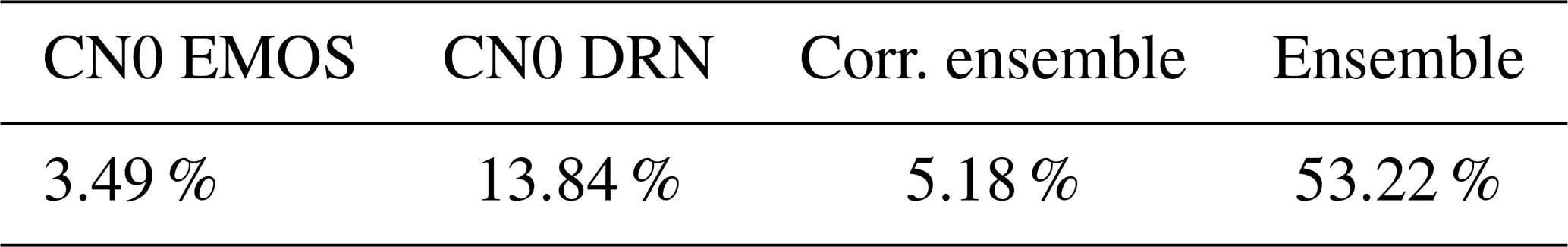
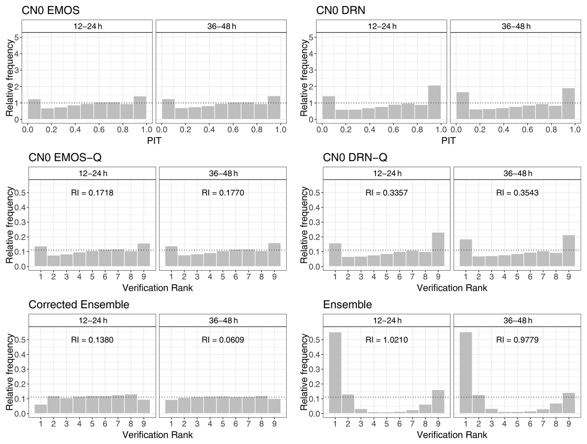
Figure 8 PIT histograms of CN0 EMOS and CN0 DRN predictive distributions and rank histograms of raw and post-processed eight-member irradiance forecasts, together with the corresponding reliability indices for lead times of 12–24 h and 36–48 h.

The verification rank and PIT histograms of Fig. 8, where we, again, consider only lead times corresponding to 12:00–00:00 UTC observations, also confirm the positive effect of statistical post-processing. First, note that the PIT histograms of the CN0 predictive distributions and the rank histograms of the corresponding samples are almost identical, which agrees with the matching CRPS and CRPSS values of Fig. 5. The highly ∪-shaped and asymmetric rank histograms of the raw WRF forecasts indicate strong underdispersion (the spread of the forecast is too low to represent the forecast error correctly) and a pronounced positive bias, respectively, resulting in reliability indices of 1.0210 (12–24 h forecasts) and 0.9779 (36–48 h forecasts). These deficiencies are substantially reduced after calibration, implying a strong improvement in reliability indices. CN0 EMOS-Q and CN0 DRN-Q forecasts are still slightly underdispersive and biased, showing reliability indices of 0.1718 and 0.1770 (CN0 EMOS-Q) and 0.3357 and 0.3543 (CN0 DRN-Q), whereas the corrected ensemble, as the slightly hump-shaped histograms indicate, is a bit overdispersive (under-confident), especially for short lead times. However, this forecast results in the lowest reliability indices of 0.1380 and 0.0609. Note that the shapes of the histograms of Fig. 8 are completely in line with the characteristics of the corresponding central prediction intervals displayed in Fig. 7. The lower coverage and narrower prediction intervals of the parametric CN0 EMOS and CN0 DRN approaches stem from their underdispersive character, while the mild overdispersion of the corrected ensemble results in wider central prediction intervals and coverage values slightly above the nominal 77.78 % level.

Finally, the MAE of the median of all five investigated predictions (Fig. 9a) and the difference in the MAE of the median from the raw WRF ensemble (Fig. 9b) convey the same message as Fig. 5. Compared to the raw ensemble, post-processing substantially improves the accuracy of the forecast median, and the corrected ensemble results in the lowest MAE values, followed by the DRN and EMOS approaches. Note that the medians of forecasts provided as full predictive distributions (CN0 EMOS and CN0 DRN) differ from the medians of their sample counterparts (CN0 EMOS-Q and CN0 DRN-Q); nevertheless, these differences are tiny as there are hardly any visible dissimilarities in the MAE values of the matching predictions.

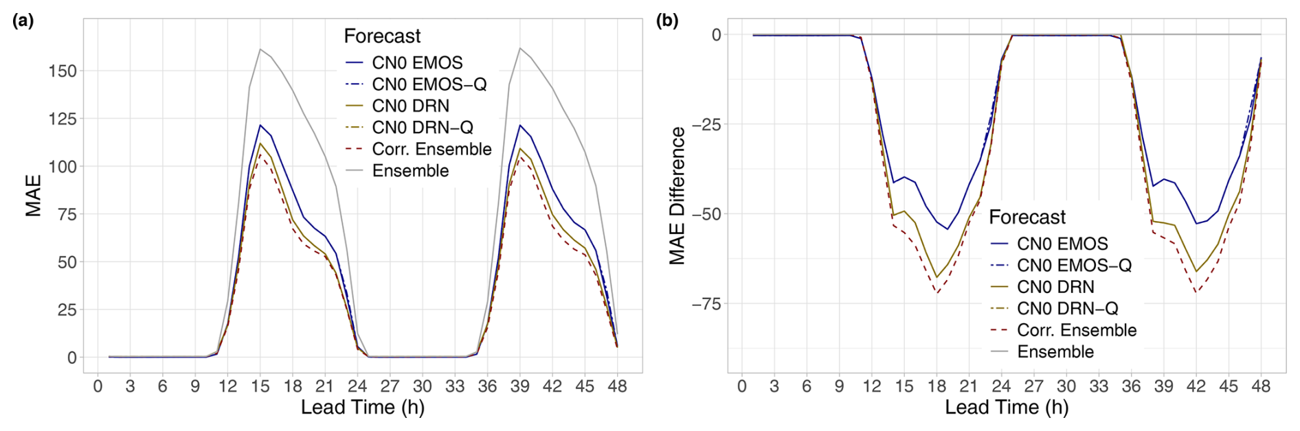
Figure 9 (a) MAE of the median of raw and post-processed irradiance forecasts and (b) difference in the MAE of the median forecasts from the raw WRF ensemble as functions of the lead time.

The above results indicate that all investigated post-processing approaches improve the calibration of probabilistic forecasts and the accuracy of point forecasts, and the corrected ensemble exhibits the best overall performance. The CN0 DRN model outperforms its EMOS counterpart in terms of both the mean CRPS and the MAE of the forecast median, but it is slightly more underdispersive, implying lower coverage and higher reliability indices.

Finally, note that we have found no evidence of a clear dependence of the predictive performance of post-processed forecasts on the location or altitude. Nevertheless, the smallest improvement, for instance, in the mean CRPS compared to the raw ensemble, can be observed at station nos. 17 (El Tololo) and 30 (Liceo Samuel Román Rojas), where the median error of the WRF forecasts is the smallest (see Fig. 2). The former is the only location where the CRPSS of the worst-performing CN0 EMOS appears to be negative.

5 Conclusions

We investigate the skill of probabilistic solar irradiance forecasts for the Atacama and Coquimbo regions in Chile. These areas play a crucial role in photovoltaic power production in the country, and our results can help obtain accurate probabilistic power forecasts. For the sake of this study, the Advanced Research module of the Weather Research and Forecasting (WRF) model was utilized to generate short-term ensemble forecasts of solar irradiance for 30 locations, with forecast horizons ranging up to 48 h and with a temporal resolution of 1 h. The forecasts comprise eight members differing in terms of the planetary boundary layer and radiation parameterization. When verified against station observations, the raw ensemble forecasts exhibit a systematic positive bias for all forecast horizons and are underdispersive; however, the magnitude of the forecast error varies substantially for the different locations.

For post-processing, we consider the parametric EMOS and DRN approaches based on a normal distribution left censored at zero and a distribution-free ensemble correction technique, where a neural network is trained to produce improved ensemble predictions. While all investigated post-processing methods substantially improve the calibration of probabilistic forecasts and reduce the MAE of the forecast median, the latter approach shows the best overall performance. From the competing parametric methods, the machine-learning-based DRN outperforms the corresponding EMOS model, which aligns with the findings of Baran and Baran (2024) and Horat et al. (2025).

As demonstrated by Horat et al. (2025), the calibration of solar irradiance ensemble predictions directly results in enhancements in the calibration of the corresponding probabilistic PV forecasts obtained by applying the PV model chains to each ensemble member separately. They also showed that even better results can be obtained by direct calibration of the PV power ensemble predictions; however, this latter approach requires the availability of the corresponding PV power production data as well, which are rather hard to obtain.

Note that all of the investigated post-processing methods provide a rather general framework and, with slight modifications, adapting them to the specialties of the input data and optimizing the training method, can be applied to any EPS and any geographical region. CN0 EMOS has already proved to be successful in calibrating 40-member ICON-EPS direct and diffuse irradiance forecasts of the DWD for three major cities in Germany (Schulz et al., 2021); 50-member GHI forecasts of the ECMWF IFS for the Jacumba Solar Project in southern California, US (Horat et al., 2025); and 11-member AROME-EPS GHI forecasts for seven solar farms in Hungary (Baran and Baran, 2024), where this post-processing approach is also in its pre-operational testing phase at the HMS. The latter two datasets have also been applied to investigate the skills of various CN0 DRN models, which, as mentioned, consistently outperformed their EMOS counterparts. The only limitation is the availability of training data; one should have enough forecast–observation pairs for reliable model training, especially for the machine-learning-based methods.

Although this first study demonstrates the weaknesses of WRF irradiance ensemble forecasts and the potential in their statistical post-processing, there is still space for further improvements in calibration. On the one hand, one might try to augment the input features of the machine-learning-based forecasts with predictions of related quantities. We have performed tests where WRF ensemble forecasts of temperature and wind speed were also included; however, the gain in forecast skill was minor, if any. On the other hand, one can test advanced neural-network-based distribution-free methods such as the Bernstein quantile network (Bremnes, 2020), where the forecast distribution is modelled with a linear combination of Bernstein polynomials or with the histogram estimation network investigated, for instance, in Scheuerer et al. (2020).

Another interesting direction would be the investigation of various multivariate post-processing methods to produce temporary consistent forecast trajectories. Here, one can think of both the state-of-the-art two-step approaches, such as the ensemble copula coupling (Schefzik et al., 2013) or the Schaake shuffle (Clark et al., 2004), where the CN0 EMOS-Q, the CN0 DRN-Q, or the corrected ensemble can serve as initial independent forecasts, and the recent data-driven conditional generative model of Chen et al. (2024).