Joint probabilistic estimates of temperature and precipitation from tree ring-based reconstructions of the last millennium

An understanding of Earth's past climate can help put current and future changes into historical context. Widely used tree ring-based drought atlases generally target the Palmer Drought Severity Index or other metrics of soil moisture and/or drought risk. These indices reflect contemporaneous meteorological conditions, and it is possible to extract information about temperature and precipitation given the existing reconstructions. Here, we present a fully Bayesian inverse method that infers a joint posterior for monthly mean temperature and precipitation given tree ring-based PDSI reconstructions from the North American Drought Atlas. The method is skillful at reconstructing early twentieth century conditions when compared to instrumental measurements from the CRU TS dataset. Moreover, the reconstructions can capture the complex temporal and multivariate covariance structure between monthly regional temperatures and precipitation. By reconstructing regional temperature and precipitation for the last millennium, we identify the driest and wettest years and decades in each region. Our results highlight the unique nature of the 1930s Dust Bowl drought in central Kansas and the late twentieth century pluvial in the North American southwest.

1 Introduction

Information from our planet's past can help us constrain natural variability in the Earth system and contextualize recent externally forced changes (PAGES 2k Consortium, 2013; Tierney et al., 2020a). However, conditions prior to the availability of quasi-global observation systems in the twentieth century must be inferred indirectly from a variety of climate proxies. One such proxy is tree rings, which have distinct advantages for reconstructing past hydroclimate conditions: they offer annual resolution, are widely available, and generally reflect well-understood responses to the surrounding environment. As a result, “drought atlases” (e.g. Cook et al., 2007, 2010b, a, 2015b; Palmer et al., 2015; Morales et al., 2020; Cook et al., 2024; Stahle et al., 2016) composed of multiple tree ring chronologies provide an important insight into hydroclimate over the last millennium.

These drought atlases generally target a single variable, most frequently the summer (June–July–August or JJA in the northern hemisphere) Palmer Drought Severity Index (Palmer, 1965; Wells et al., 2004). While this index is most commonly abbreviated PDSI, here we denote it D for brevity. This index reflects a complex mix of meteorological conditions (e.g., inputs from precipitation and losses due to evapotranspiration calculated as a function of temperature, humidity, wind speed, radiation, etc. Dai, 2011) that occur not only over the summer, but over the previous year or years as well. This means that the reconstructed D holds information about more than just soil moisture and drought risk: it can also be used to infer past temperatures and precipitation amounts–albeit with considerable uncertainty.

Bayesian inference has always been a powerful tool for drawing conclusions from sparse data (Gelman et al., 1995), and recent methodological innovations (Hoffman and Gelman, 2014), new computing environments (Kumar et al., 2019; Abril-Pla et al., 2023; Bastien F., 2022) and increased processing power (Brooks, 2003) have made fully Bayesian approaches more tractable and useful. In paleoclimate, these techniques offer a probabilistic framework that can incorporate uncertainties in both proxy data and model parameters (Haslett et al., 2006; Tingley and Huybers, 2010), leading to more robust estimates of past climate states. Unlike traditional methods that often produce deterministic outputs, Bayesian reconstructions result in full posterior distributions, allowing for nuanced interpretations of uncertainty.

As such, Bayesian methods are widely used in paleoclimatology for tasks such as estimating global mean temperature from networks of proxies (Tierney et al., 2020b) and assimilating multiple proxy measurements to generate reconstructed fields (Steiger et al., 2018). Most of these methods utilize the output of general circulation models (GCMs) to generate prior distributions of variables and capture existing and expected covariance structures, and their conclusions may depend heavily on the prior used (Annan et al., 2022).

Here, we present a simple inverse method to reconstruct regional temperature and precipitation using available tree-ring-based drought atlases that does not rely on the use of GCMs. This method can be used to complement, not replace, existing reconstruction techniques. Our goal here is to extract as much information as possible from the published drought atlas record using a method that is interpretable, does not rely on GCMs, and incorporates uncertainty from multiple sources.

2 Methods

To reconstruct past regional temperatures and precipitation amounts, we use the North American Drought Atlas (NADA, Cook et al., 2007, 2010b). Developed through extensive dendrochronological sampling, NADA provides a gridded spatial reconstruction of hydroclimate conditions across North America, with good reconstruction fidelity extending back 500–1000 years. This dataset has allowed for detailed analyses of drought frequency, severity, and spatial extent prior to the onset of instrumental records (Fye et al., 2003; Cook et al., 2014), identification of long-term drought patterns including multi-decadal megadroughts (Cook et al., 2009, 2016), and comparisons of recent hydroclimatic extremes within a broader temporal framework (Stahle et al., 2007; Cook et al., 2015a; Marvel and Cook, 2022).

To demonstrate our method, we choose to reconstruct monthly temperature and precipitation from the NADA in the grid cells closest to three locations:

• Dodge City, Kansas (DCK): (37.75° N, −100.00° W). This location in the Central Plains is regarded as the heart of the Dust Bowl (Worster, 2004).

• Red Mesa, Arizona (RMA): (37.00° N, −109.38° W). Near the Four Corners region of the southwestern US, this is the epicenter of historical megadrought activity (Cook et al., 2007).

• Sonora Junction, California (SJC): (38.35° N, −119.45° W). Located in the Sierra Nevada mountains near the West Walker River, this is another hotspot of major drought activity (Williams et al., 2020)

Not only are these locations hotspots of past drought activity, the climatologies of precipitation differ greatly across these three sites: in DCK precipitation is highest in spring and summer, in SJC almost all precipitation arrives in the winter, and in RMA precipitation is more evenly distributed throughout the year (Fig. 1).

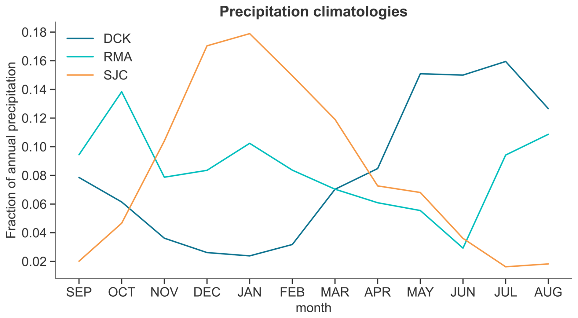
Figure 1 Different regions have different precipitation climatologies. Monthly mean precipitation totals divided by the total annual mean precipitation for Dodge City, Kansas (dark blue), Red Mesa, Arizona (cyan) and Sonora Junction, California (orange).

For training and validation, we use monthly mean temperature (T) and precipitation (P) from the CRU TS instrumental dataset (Harris et al., 2020), which spans 1901–2023 and is based on station observations which are interpolated and corrected for biases such as station inhomogeneity and gauge undercatch. For each year y, we construct a column vector of monthly standardized temperature and precipitation $M\left(y\right)=(T_{\mathrm{Sep}}\mathrm{\dots }{T}_{\mathrm{Aug}},P_{\mathrm{Sep}}\mathrm{\dots }{P}_{\mathrm{Aug}}{)}^T$ (where September–December values are taken from the previous year y−1) in order to capture causal relationships between monthly meteorology and JJA D from the NADA. Monthly temperatures are assumed to be normally distributed and are standardized by calculating the z-score, while monthly precipitation totals are converted into a standardized precipitation index by fitting a gamma distribution and standardizing the cumulative probabilities (Guttman, 1999). We split both meteorology M and drought index D into training (1950–2005) and validation (1902–1949) periods.

Our task is to reconstruct the 24-dimensional column vector M(y) from known (tree ring-derived) D(y) as represented in the NADA. We split this process into three elements: first, we estimate the parameters of a forward model that yields D given observed values of M over the training period. Second, we estimate a prior on M that captures the observed covariance structure between monthly temperatures and precipitation amounts. Third, we combine these to yield a full posterior for unobserved monthly temperatures and precipitation over the last millennium.

2.1 Incorporating proxy uncertainty

Paleoclimate datasets are necessarily based on indirect “proxy” measurements of past global conditions- in the case of drought atlases, tree ring chronologies. While the ability of tree rings to capture past and present drought risk has been extensively validated, the use of proxies to reconstruct the “true” values of any index is a source of uncertainty in the final estimates. To model this, we compare the reconstructed D_proxy in the NADA to instrumental D provided by CRU over the training period:

$$\begin{array}{}\text{(1)}& D_{\mathrm{proxy}}\sim N(D,{\mathit{\sigma }}_{\mathrm{proxy}}).\end{array}$$

CRU TS and NADA data over the training period is used to infer a posterior distribution for the uncertainty σ_proxy, which then propagates through to the posterior distribution of the reconstructed M. Over the reconstruction period, where we have no instrumental data, the “true” value D is latent, and we have only D_proxy, which we assume can be described by the model in Eq. (1). We thus use a hierarchical model in which proxy-based reconstructions are used to infer a posterior for the instrumental D, which in turn can be used to reconstruct past temperature and precipitation.

2.2 Forward model

Summer soil moisture, and by extension JJA PDSI, depends on temperature and rainfall in the preceding year. We expect the dependence to be sensitive to the monthly climatology of temperature and rainfall in each region. Moreover, we expect the soil in some regions to retain at least some “memory” of its value the year before, so that a dry year is likely to be followed by another dry year and a wet year by another wet year (Cook et al., 2022).

Thus, we assume that D(y) in a given year depends linearly on contemporaneous meteorological conditions M(y) and on its value D(y−1) in the previous year. We express this as a conditional distribution

$$\begin{array}{}\text{(2)}& D\left(y\right)\sim N\left({\mathit{\beta }}^T\mathit{M}\right(y)+\mathit{\rho }D(y-\mathrm{1}),\mathit{\sigma }).\end{array}$$

where β is a vector of regression coefficients, ρ the lag-1 autocorrelation between D and its previous-year value, and σ is a Gaussian white noise term. We place N(0,1) priors on ρ and on each component of β, and use a half-normal prior N⁺(1) for σ.

2.3 Learning a prior from observations

Regional temperature and precipitation are affected by multiple drivers, from the local (e.g. soil moisture feedbacks (Seneviratne et al., 2010; Miralles et al., 2014)) to the remote (e.g. the influence of SST patterns (Kushnir et al., 2016; Schubert et al., 2010; Zhang et al., 2023)) and variability in the atmospheric circulation (Burgdorf et al., 2019; Cook et al., 2024). The impacts of these drivers are apparent on multiple timescales: during an El Niño event, for example, regional temperature and rainfall may remain elevated or suppressed for months, whereas the effects of short-term synoptic events may last only a few hours or days. As a result, monthly mean regional temperatures and rainfall are expected to co-vary with one another in non-trivial ways. We wish to capture the inherent temporal structure and relationships between T and P in a prior distribution for past meteorology P(M) that reflects the relationships apparent in present-day conditions.

2.3.1 Inferring past conditions from a warming present

In reconstructing past meteorological conditions we are faced with an unavoidable problem: all current weather occurs against the backdrop of rapid global warming. Because current global temperatures are unprecedentedly warm, the basic assumption of all learning models (that the training data resembles the validation data) is invalid. This means we require some known functional form to interpolate between present and past data. Here, we assume that current regional monthly mean temperatures and precipitation amounts scale with the global mean temperature G(t). Over the training and validation periods we use the GISS Surface Temperature Analysis (GISTEMP v4, Lenssen et al., 2019) to estimate the annual global mean temperature anomaly G relative to a 1951–1880 baseline.

Initially, we assume no information about the global mean temperature prior to the instrumental period. We treat the last-millennium temperature (denoted G₁₀₀₀) as a random variable:

$$G_{\mathrm{1000}}\sim N(\mathit{\mu },{\mathit{\sigma }}_T)$$

where μ is the average global mean temperature anomaly (relative to the 1950–1980 GISTEMP base period) and σ the standard deviation of the detrended 1900–2005 GISTEMP time series.

We also want to capture a nontrivial covariance structure between T and P in different months and between each other. Temperature and precipitation have common drivers, and therefore we might expect these variables to be correlated in different regions. We model this with a 24×24 matrix Σ that represents the covariance structure of monthly temperature and precipitation in a given year due to unforced internal variability.

Our model for local meteorological conditions M is thus

$$\begin{array}{}\text{(3)}& M\left(y\right)\sim MN(\mathit{\gamma }G,\mathrm{\Sigma })\end{array}$$

where γ is a 24-element vector of scaling factors representing the dependence of regional monthly mean temperature and precipitation on global mean temperatures.

We place an Lewandowski–Kurowicka–Joe (LKJ) prior (Lewandowski et al., 2009) on the internal variability covariance matrix Σ with η=1 and N⁺(1) distributions for the standard deviations. The LKJ prior is commonly used for covariance matrices because it provides a flexible and interpretable way to model correlation structures by controlling the concentration around the identity matrix, ensuring valid, positive-definite correlation matrices. We additionally place standard normal priors on all components of γ.

2.4 Calculating the posterior for unobserved M

In the absence of noise, we could obtain estimates for the unknown M given D by simply inverting the forward model (Eq. 2). However, the existence of random variability means the inverse problem is ill-posed. To solve it, we reformulate the reconstruction of M given D as a Bayesian inference problem. This allows us to use training data, the forward model, and our model of a priori information to extract information and assess the uncertainties.

In this framework, the complete solution to the inverse problem is the posterior distribution

$$\begin{array}{}\text{(4)}& P\left(\mathit{M}\right|D,\mathit{R})={\displaystyle \frac{P\left(D\right|\mathit{M},\mathit{R}\left)P\right(\mathit{M}\left|\mathit{R}\right)}{P\left(D\right|\mathit{R})}}\end{array}$$

where $\mathit{R}=(M_{\mathrm{train}},D_{\mathrm{train}})$ is the full set of training data. The likelihood is given by

$$\begin{array}{}\text{(5)}& P\left(D\right|\mathit{M},\mathit{R})=\int P(D|{\mathit{\theta }}_{\mathrm{F}},\mathit{M})P\left({\mathit{\theta }}_{\mathrm{F}}\right|\mathit{R})\mathrm{d}{\mathit{\theta }}_{\mathrm{F}}\end{array}$$

where ${\mathit{\theta }}_{\mathrm{F}}=(\mathit{\beta },\mathit{\rho },\mathit{\sigma },{\mathit{\sigma }}_{\mathrm{proxy}})$ are the parameters of the forward model and P(θ_F|R) the posterior distributions given the training data.

In Bayesian inversion problems, the prior distribution does the work of regularization. It turns an ill-posed problem into a well-posed one, encapsulates the covariance structure, and makes explicit prior assumptions about the solution. Our prior assumptions are uncertain, as we are not perfectly sure how much of observed variability in M_train is a forced response and how much is internal variability. This means that the prior

$$P\left(M\right|R)=\int P(M|{\mathit{\theta }}_M,R)P\left({\mathit{\theta }}_M\right|R)\mathrm{d}{\mathit{\theta }}_M$$

is uncertain and conditioned on the observed training data R and the posterior values of the parameters ${\mathit{\theta }}_M=(\mathit{\gamma },\mathrm{\Sigma })$. The resulting posteriors for the unobserved M therefore reflect multiple uncertainties: the covariance structure of internal variability, the dependence of D on its value in previous years, and the relationships between monthly temperature, precipitation, and D.

Bayesian inference was performed using the PyMC probabilistic programming framework (Martin, 2018; Abril-Pla et al., 2023). After specifying the above prior distributions and likelihood functions within the model context, posterior distributions were estimated via Markov Chain Monte Carlo (MCMC) sampling. The PyMC sample() function was used to draw samples from the posterior distribution, employing the No-U-Turn Sampler (NUTS, Hoffman and Gelman, 2014), an adaptive variant of Hamiltonian Monte Carlo.

3 Results

3.1 Training

3.1.1 How do instrumental temperature and precipitation over the training period relate to summertime PDSI?

Figure 2a shows the posterior distributions for the regression coefficients β in the DCK region. Over the training period, anomalously high summertime D is robustly associated with low late spring and summertime temperatures (negative values of β) and high precipitation (positive values of β) , especially in the spring and summer when this region receives the bulk of its precipitation. The posterior distribution for the white noise term σ is substantially shifted away from 1, indicating that the observed variability in D is not wholly explained by white noise, while the posterior for ρ is robustly nonzero, indicating a substantial soil moisture memory (Fig. 2b).

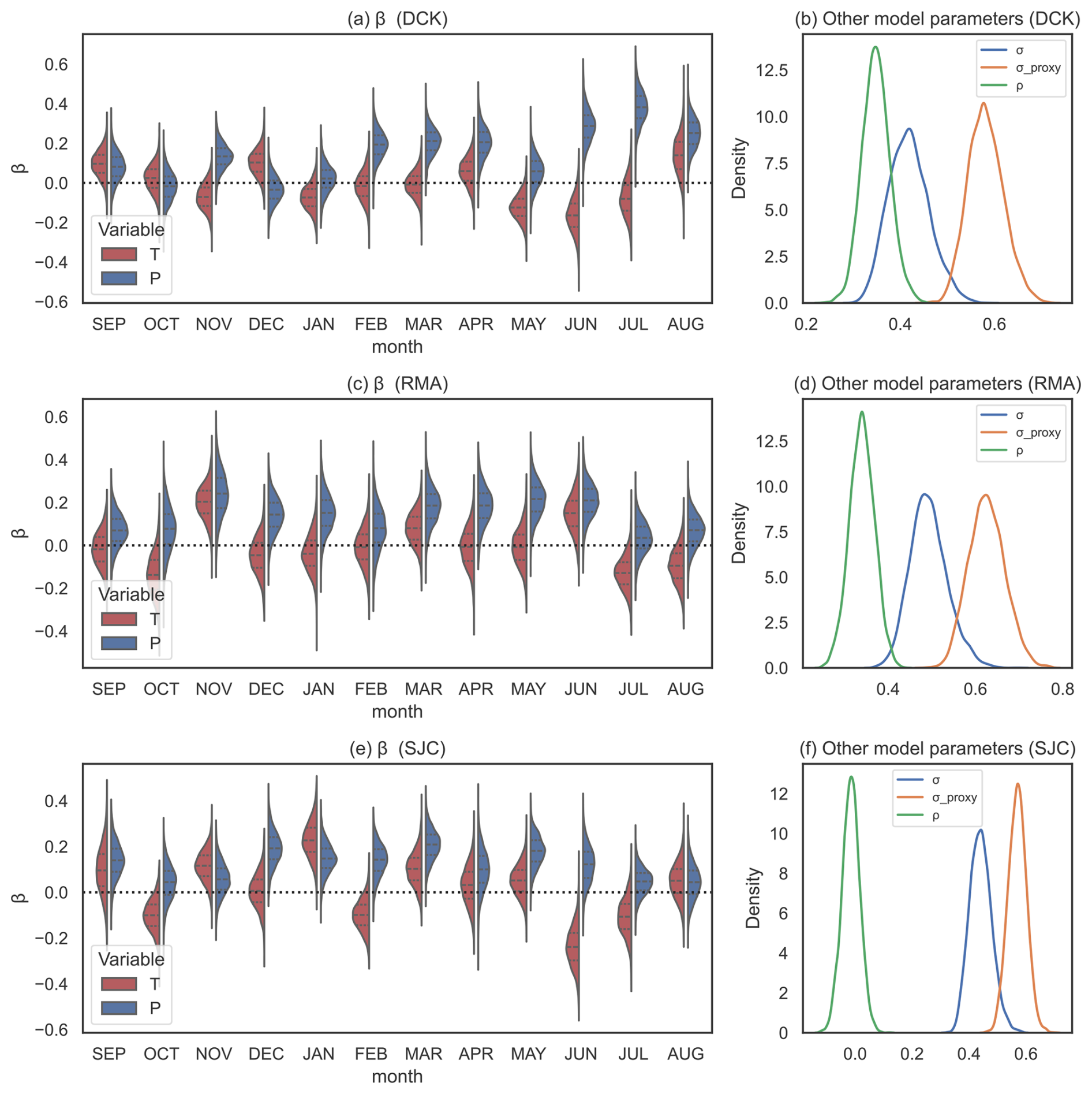
Figure 2 How does the reconstructed Palmer Drought Severity Index relate to the instrumental temperature and precipitation? Each panel shows the posterior distributions for different parameters in the forward model. Panel (a) shows the components of the monthly regression coefficients for temperature (red) and precipitation (blue) in Dodge City, Kansas. Black horizontal lines on the red and blue distributions indicate the quartiles of the posterior distributions. Panel (b) shows the white noise term σ (blue) and the lag-1 autocorrelation ρ (orange) for the model fitted to Dodge City, Kansas. Panel (c) shows the same quantities as (a), but for Red Mesa, Arizona. Panel (d) shows the same quantities as (b), but for Red Mesa, Arizona. Panels (e) and (f) show the same quantities as in panels (a) and (b), respectively, but for Sonora Junction, California.

Rainfall in RMA is more evenly distributed throughout the year, and D in this region is more sensitive to precipitation in the fall and winter than in DCK (Fig. 2c). As in DCK, the autocorrelation ρ is positive and robustly nonzero, indicating that the reconstructed D in this region, as in DCK, depends on its value in the prior year (Fig. 2d).

In SJC, the vast majority of precipitation occurs in the fall, winter and spring, and thus the posteriors for β are strongly positive in these months (Fig. 2e). While very little precipitation typically falls in June, any amount of rainfall in the early summer can strongly influence JJA D, and the posterior distribution of β for June is also shifted to positive values. High May and June temperatures in this region are strongly associated with drier D. Interestingly, the posterior for ρ in this region is not substantially shifted away from zero; D in SJC does not appear to depend strongly on its previous value, at least during the training period.

3.1.2 Evaluating the forward model

In all three regions, the simple linear forward model (Eq. 2) is very skillful at capturing the observed variations in D over the training period (Fig. 3); almost every year lies within the “likely” range of the model, defined as the 66 % highest-density interval of the posterior predictive distribution. The forward model outperforms more complex models such as a neural net and a tree-based regression (not shown) and has the advantage of being highly interpretable.

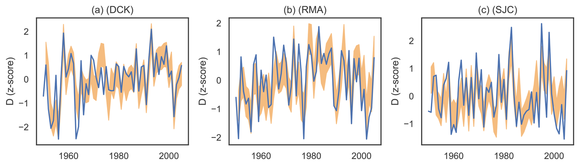
Figure 3 The forward model is a good fit to the observed training data. Panel (a) shows the 66 % highest-density interval for the posterior predictive distribution (brown shading) and “observed” (NADA) D (brown lines) over the training period for Dodge City, Kansas. Panel (b) shows the same quantities for Red Mesa, Arizona. Panel (c) shows the same quantities for Sonora Junction, California.

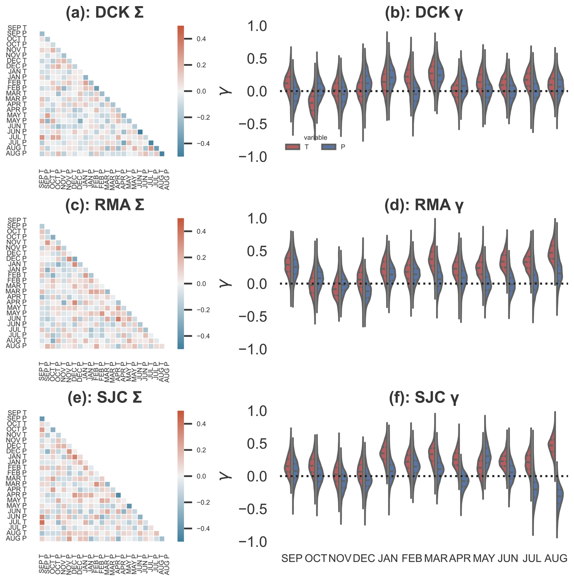
Figure 4 How do monthly mean temperature and precipitation co-vary? Panel (a) shows the posterior mean covariance matrix Σ for Dodge City, Kansas. Panel (b) shows the posterior distributions for the regression coefficients γ, which capture the dependence of regional T (red) and P (blue) on global mean temperature. Dashed black lines indicate quartiles of the posterior distributions. Panels (c) and (d) show the same quantities as (a) and (b), but for Red Mesa, Arizona. Panels (e) and (f) show the same quantities as (a) and (b), but for Sonora Junction, California.

Figure 4a shows the posterior mean covariance matrix Σ for DCK, which captures the observed temporal relations between monthly temperature and precipitation in the training data. Of note are the strong anti-correlations between T and P in the same month, suggesting that in DCK, warm months are generally accompanied by precipitation deficits and vice versa. The relationships between temperature in a given month and the temperature in preceding or successive months are fairly weak in this region: the strong correlations between temperatures in different months observed over the training period are likely driven by a common response to increasing global mean temperatures. We remove this common response by incorporating the γG term. This contrasts with the results for RMA and SJC (Fig. 4c and e), in which wintertime monthly temperatures are correlated with temperatures in the adjoining months, likely reflecting the persistent influence of ENSO variability in these regions.

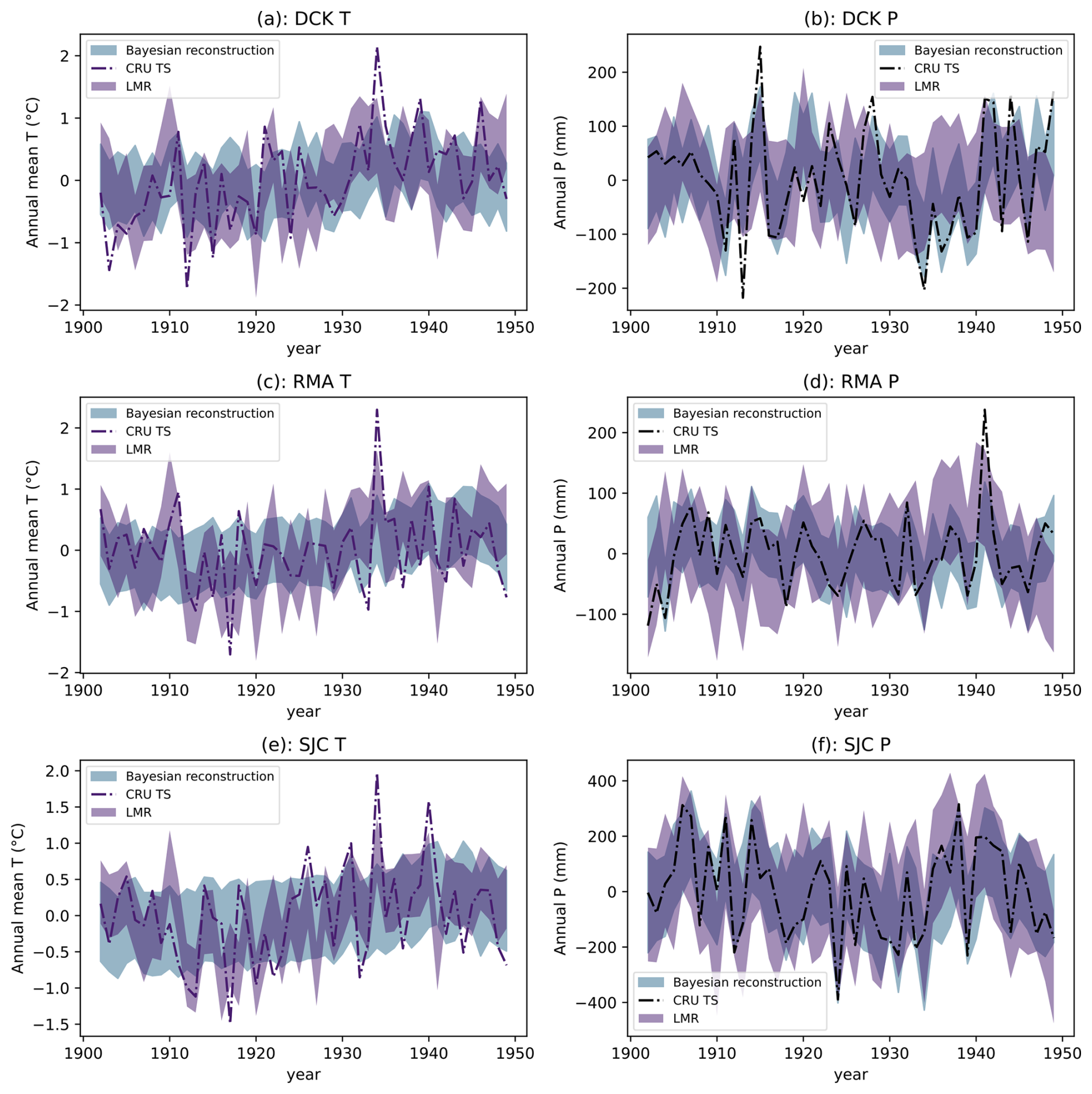
Figure 5 The reconstruction method performs well over the validation period. Panel (a) shows the CRU instrumental (black dashed line), reconstructed (66 % HDI range, light blue), and Last Millennium Reanalysis annual mean and 1σ uncertainty (purple) regional annual temperature anomaly in Dodge City, Kansas. For CRU and the reconstruction presented here, “annual mean” refers to the September–August average, while the Last Millennium Reanalysis annual mean is the January–December average. Panel (b) shows CRU (black dashed line), this reconstruction (light blue), and LMR annual precipitation totals in Dodge City, Kansas. Panels (c) and (d) show the same quantities as (a) and (b), but for Red Mesa, Arizona. Panels (e) and (f) show the same quantities as (a) and (b), but for Sonora Junction, California.

Monthly temperatures in all three regions have risen along with global mean temperatures. In DCK, the warming has been relatively muted and mostly concentrated in the winter months (Fig. 4b). In RMA, temperatures have risen along with global temperatures throughout the year, with the exception of October–December. This is also the case in SJC, although summer temperatures in this region have been more strongly associated with rising G. Regional precipitation appears largely insensitive to G with the exception of decreases in the summer months in SJC, although given the climatology of summer rainfall in this region this is likely dominated by small fluctuations in already-miniscule values.

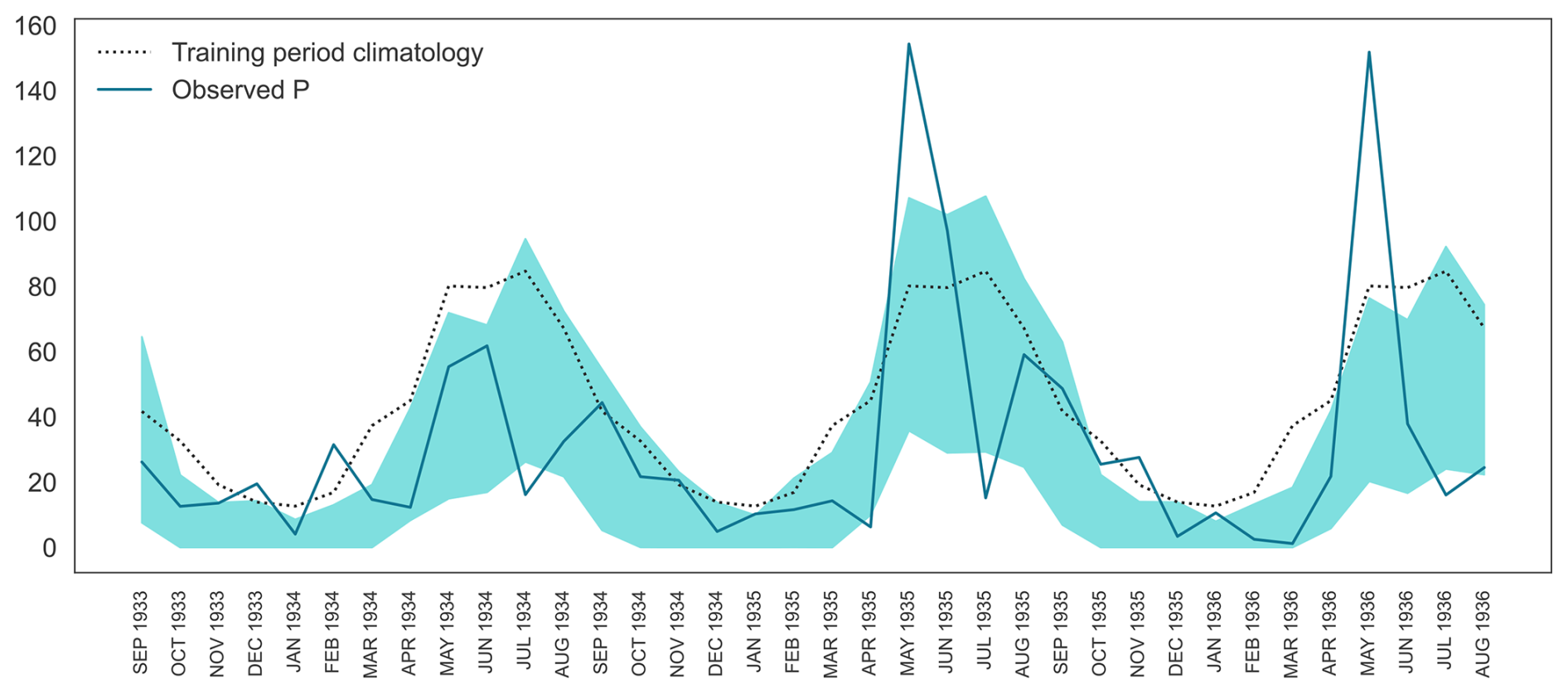
Figure 6 Monthly precipitation reconstructions. Instrumental monthly total precipitation (blue line), monthly climatologies (dotted black line) and the 95 % highest-posterior-density interval (shaded blue region) of reconstructed precipitation in Dodge City, Kansas from September 1933–August 1936.

3.2 Validation

Over the validation period, our annual mean precipitation reconstructions in all three regions compare well with CRU TS instrumental data (Fig. 5). The correlations between the posterior mean and the CRU observations are 0.72, 0.72, and 0.78 for DCK, SJC, and RMA respectively. We note that our “annual means” refer to the average temperature from September (in the previous year) to August (in the current year). There is substantial overlap between our annual mean precipitation posteriors with results from the Last Millennium Reanalysis (Tardif et al., 2019), a product derived by assimilating multiple proxy records (although these annual means are for the calendar year). In particular, our reconstruction is better able to capture the Dust Bowl drought in the DCK region in the 1930s, and largely mirrors the instrumental observed precipitation variability. In all regions, the instrumental precipitation values fall within the reconstructed “likely” range (defined as the 66 % highest-posterior density interval for our reconstruction and ±1σ for the LMR) of both reconstruction datasets for most years. Our model is, however, less able to capture the observed variations in regional temperature: while the correlations between the posterior mean and CRU regional temperatures are 0.54, 0.31, and 0.4 for DCK, SJC, and RMA respectively. The LMR reconstruction exhibits far more year-to-year variability in annual regional temperature. This is due to the fact that our Bayesian method uses a single source of input (the tree-ring reconstructed D) that is far less sensitive to local temperatures than precipitation amounts. It is therefore no surprise that the multi-proxy LMR product captures more interannual variability over the validation period. Despite this, our method is not completely without skill in reconstructing regional temperatures- while it does not capture the magnitude of extreme heat events in the 1930s, the posterior temperatures in those hot years do appear to be shifted towards higher values. Moreover, our model provides joint posteriors, partitioning observed or reconstructed D into the combinations of temperature and precipitation that might have caused those conditions.

Annual averaging of the reconstructions reduces uncertainty, but the monthly precipitation reconstructions still appear somewhat skillful. Figure 6 shows the likely range of the reconstructed monthly precipitation, the instrumental monthly precipitation, and the instrumental climatology over the training period over three years at the height of the Dust Bowl drought.

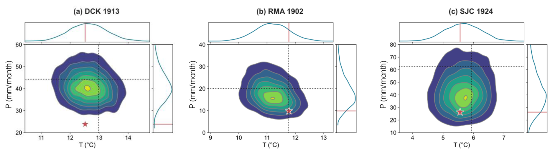
Figure 7 How well does the reconstruction capture low precipitation extremes? Panel (a) shows the joint posterior distribution (contour lines) for the reconstructed annual (September–August) temperature and precipitation for 1913, the year of lowest recorded precipitation (as recorded in CRU instrumental data) over the validation period in Dodge City, Kansas. Marginal PDFs are shown on the top (for T) and right (for P). Annual mean climatologies for T and P are shown as dashed lines. Panels (b) and (c) show the same thing, but for Red Mesa, Arizona in 1902 and Sonora Junction, California in 1924.

While the reconstruction fails to capture the unusually large rainfall rates in May 1935 and 1936 or the subsequent anomalously low values in June of those years, it suggests that rainfall throughout the rainy season as likely well below normal in 1934 and 1936 – as seen in the instrumental record.

To understand how well the model captures extreme values of temperature and precipitation, we examine the year (in each region) over which 1901–1949 precipitation was lowest. Figure 7 shows the joint posterior for annual mean T and P in the driest year for each region.

1913 was the year of lowest recorded precipitation in DCK, despite being slightly colder than average. Our reconstruction model suggests that both annual mean rainfall and temperature were both slightly below normal, although it tends to underestimate the magnitude of the precipitation anomaly (Fig. 7a). The instrumental temperature lies well within the likely range of temperatures reconstructed by the model. However, while the reconstructions indicate lower-than-average precipitation, the instrumental value lies in the far tail of the reconstructed posterior (right-hand marginal plot, Fig. 7a). This is likely because the NADA records a D that is less than 0.2 standard deviations below the mean, possibly due to near-average rainfall in April and June 1913 (Fig. 8).

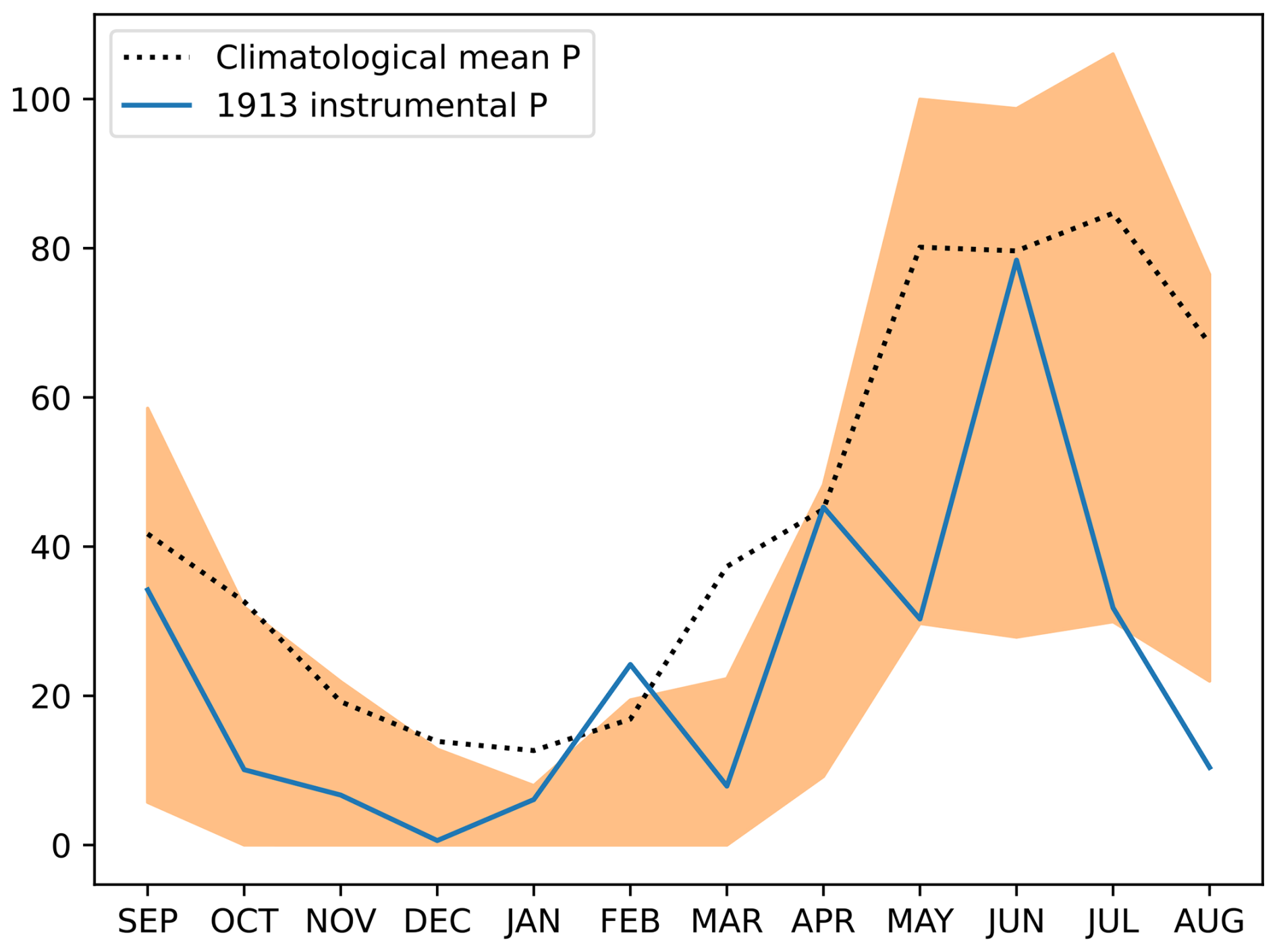
Figure 8 Monthly precipitation deficits in the driest year on record Shown is monthly mean precipitation for Dodge City, Kansas in 1913, the driest (lowest P) year on record. Shown are the training period climatological mean (black dashed line), the 95 % highest-posterior-density inverval of the reconstructions (shaded orange region) and the instrumental precipitation from CRU TS (blue line).

In RMA, 1902 was the driest year in the precipitation instrumental record. The reconstructed posterior suggests lower-than-average precipitation and slightly lower-than average temperature; the instrumental data indicates roughly average temperatures and well-below average precipitation (Fig. 7b).

In SJC, 1923 was the driest year, and the reconstructions suggest far-below-average precipitation and slightly below-average temperature. The instrumental data lie near the center of the reconstructed posterior (Fig. 7c).

3.3 Reconstructions

Figure 9 shows the reconstructed annual mean temperature and precipitation since 1000 CE for all three locations, using the “base” model in which global mean temperature G over the last millennium is treated as an unknown random variable.

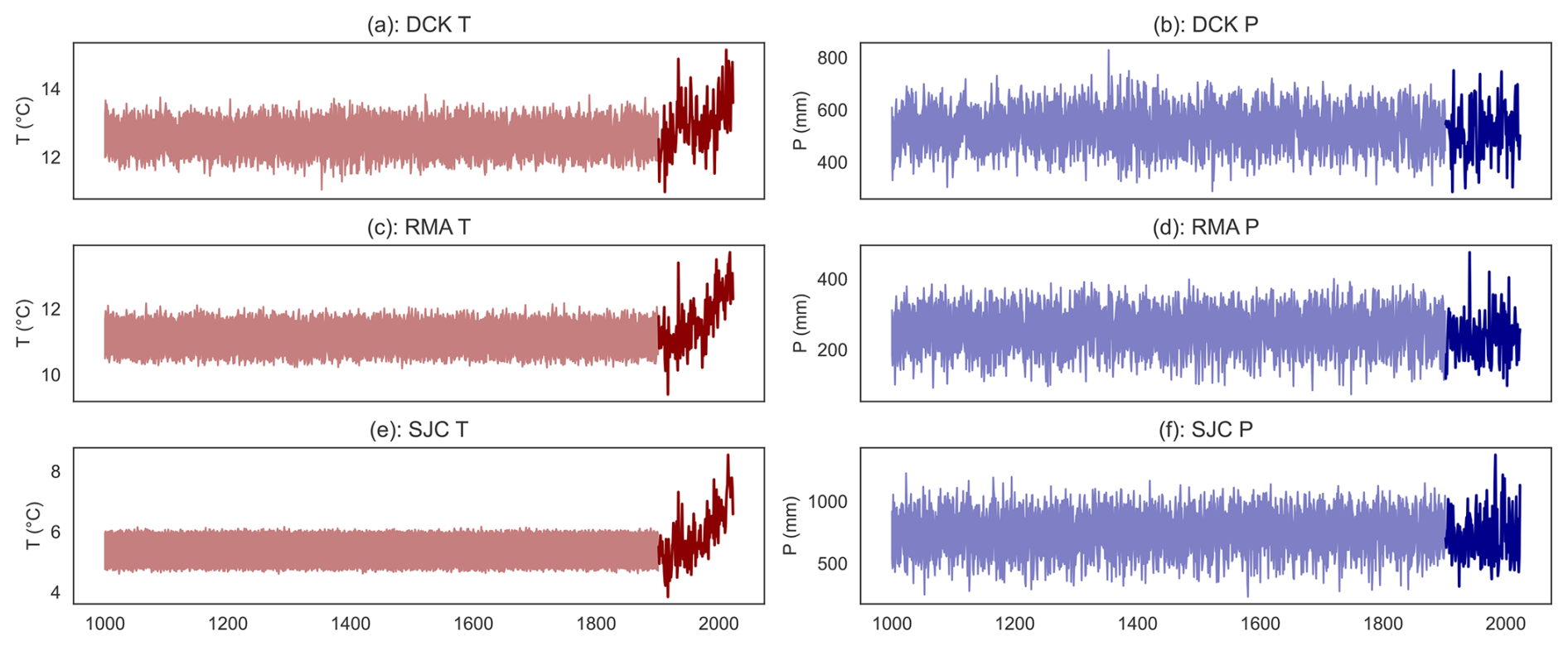
Figure 9 Last-millennium reconstructions show more interannual variability in precipitation than in temperature. Panel (a) shows the reconstructed likely (66 % HDI) range of temperature (red shading) and precipitation (blue shading) over 1000–1901 for Dodge City, Kansas. Instrumental (CRU TS) measurements from 1901–2023 are shown as solid lines. Panels (c) and (d) show the same quantities but for Red Mesa, Arizona. Panels (e) and (f) show the same quantities for Sonora Junction, California.

The tree ring-based D is far less informative about past temperatures than about past precipitation; unsurprising given that D over the training period is observed to be more strongly related to precipitation (Fig. 2). Additionally, regional temperature is far more likely to rise and fall in tandem with global mean temperatures, which we assume to be an unknown random variable over the reconstruction period. However, in keeping with multiple previous studies (e.g. Gillett et al., 2021; Santer et al., 2013; Hegerl et al., 1997), our reconstructions show temperatures in all three regions exceeding and remaining above the likely range of pre-industrial temperatures by the present day. By contrast, there are no pronounced upward or downward trends in recent regional precipitation relative to the reconstructions.

The T reconstructions exhibit very little year-to-year variability, especially in SJC. This is because the growing season Palmer Drought Severity Index in this region (the target variable for the drought atlases) is relatively insensitive to temperature, and thus provides very little information about past temperatures. Additionally, the base model uses a standard normal model for the (unknown) global mean temperature over the past millennium. As a result, very little information about regional T is provided by D, and none at all by G. Thus, in SJC (and to a certain extent in other regions), the reconstruction essentially tells us nothing that could not be inferred from assuming temperature to be white noise with the same amplitude as the detrended observations.

The situation is improved somewhat when we explicitly treat G₁₀₀₀ as a covariate (Fig. 10) by using reconstructed global mean temperature from the Last Millennium Reanalysis. Because temperatures in all three regions do tend to scale with the global mean temperature, including more information does allow us to reconstruct more complex modes of temporal variability in regional T, although this information is coming from the global mean temperature rather than the reconstructed local PDSI. Also shown in Fig. 10 are the regional reconstructions from the grand ensemble mean of the Last Millennium Reanalysis (with the caveat that unlike our September–August reconstructions, these are for the calendar year). Our method, in which information comes only from local D and global G, does not show the same amplitude of regional temperature variability as the LMR- to be expected, as the latter dataset draws information from multiple proxies. What is surprising, however, is just how much information can be extracted from just D and G, particularly for precipitation.

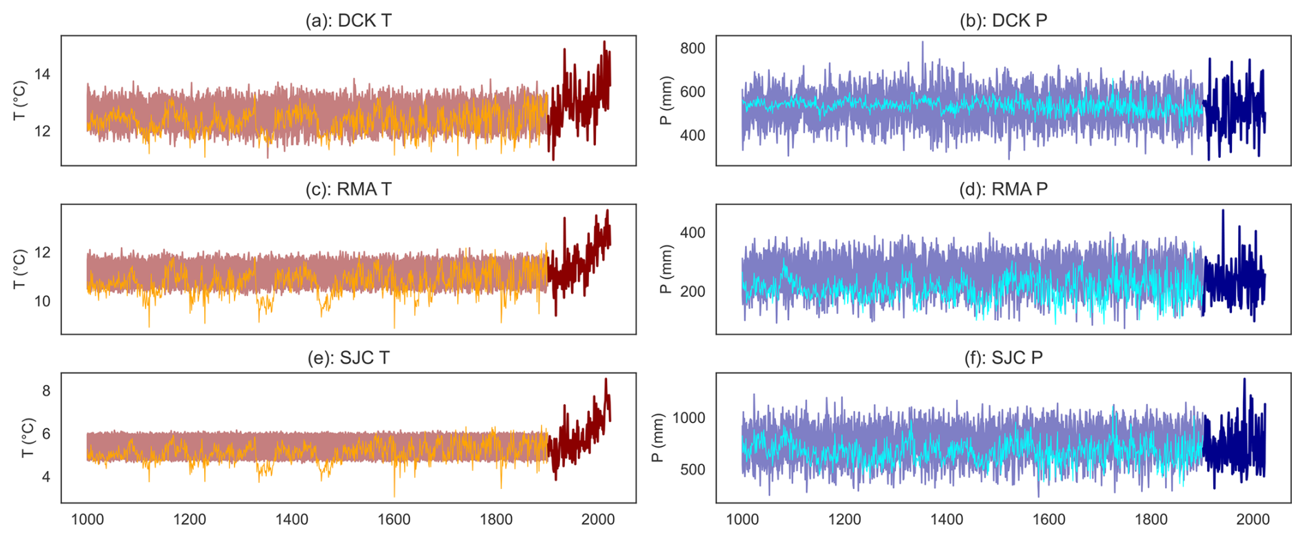
Figure 10 Including reconstructed global mean temperature as a covariate increases variability in temperature reconstructions. Panel (a) shows the reconstructed likely (66 % HDI) range of regional temperatures in Dodge City, Kansas (red shading) over 1000–1901 using a reconstruction model in which global mean temperature G₁₀₀₀ is taken from the Last Millennium Reanalysis ensemble. Also shown are regional temperatures (orange) from the Last Millennium Reanalysis grand ensemble mean. Panel (b) shows the reconstructed likely (66 % HDI) range of precipitation in Dodge City, Kansas (blue shading) over 1000–1901 using a reconstruction model in which global mean temperature G₁₀₀₀ is taken from the Last Millennium Reanalysis. Also shown are regional precipitation amounts (cyan) from the Last Millennium Reanalysis grand ensemble mean. Panels (c) and (d) show the same quantities but for Red Mesa, Arizona. Panels (e) and (f) show the same quantities for Sonora Junction, California.

3.3.1 Identifying extreme years

Our reconstruction can also be used to identify years or seasons of extreme precipitation in the past, and to compare these to the more recent period. Our posteriors for regional temperature and precipitation contain 4000 realizations, which we can then concatenate with CRU TS instrumental data over the training and reconstruction periods. The number of times any given year appears as the wettest/driest (or hottest/coldest) gives us an estimate of the probability that year was the most extreme in the record.

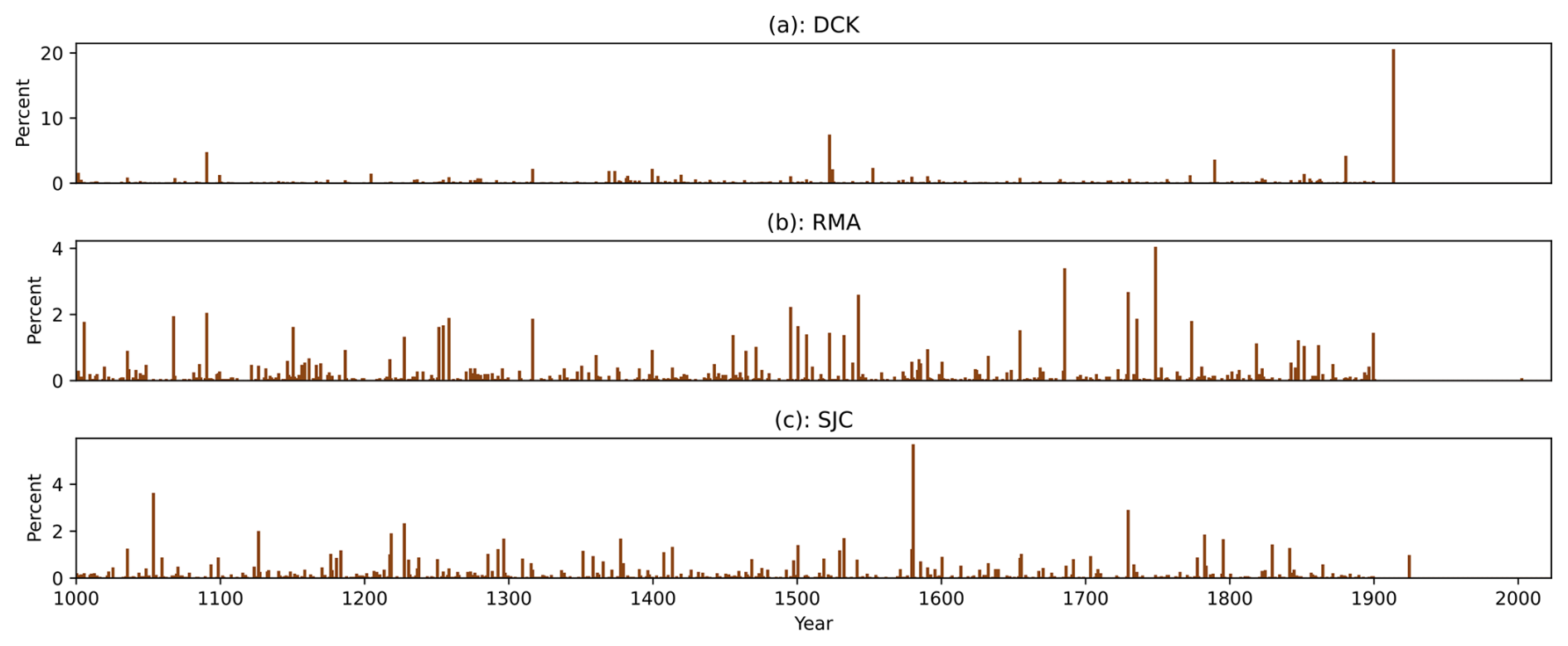
Figure 11 Driest years on record. Panel (a) shows the probability of a given year being the driest (lowest precipitation) decade since 1000 CE in Dodge City, Kansas. Panel (b) shows the same for Red Mesa, Arizona. Panel (c) shows the same for Sonora Junction, California.

For example, using the “base” reconstruction, in DCK the lowest-precipitation year in the 1000–1901 reconstruction period was likely 1522. By contrast, the year with lowest summertime D in the NADA is 1880. Our model tends to associate 1522 with lower precipitation because the previous years recorded very high D, requiring a more strongly negative precipitation anomaly to decrease it. As illustrated in Fig. 7a, 1913 was the lowest precipitation anomaly over the instrumental period. There is a 23 % chance that it was the lowest precipitation anomaly since at least 1000, while there is a 13 % chance that the driest (lowest-P) year since 1000 was 1522 (Fig. 11a).

In other regions, the driest (lowest P) years did not necessarily occur over the instrumental period. In RMA, there is only a 0.05 % chance the driest year occurred post-1901. In this region the most likely driest years on record were 1748, 1685, 1729, and 1542. In SJC, there is a 1 % chance that the driest year occured post-1901, with the most likely driest years being 1580, 1053, 1729, and 1126.

Applying a ten-year rolling mean to the posteriors for P allows us to calculate the decades in which precipitation was lowest. In DCK, there is a 71 % chance that 1931–1940 was the driest (lowest precipitation) decade on record: interesting, because the 10 year window with lowest average D in the NADA is 1855–1864. No one ten-year period particularly stands out as the driest on record in RMA: the most-often identified decade 1142–1151 is the driest ten-year period in 3 % of the samples, corresponding to a notable megadrought in the southwestern US. In SJC, there is a 37 % chance that 1924–1933 was the driest ten-year period on record.

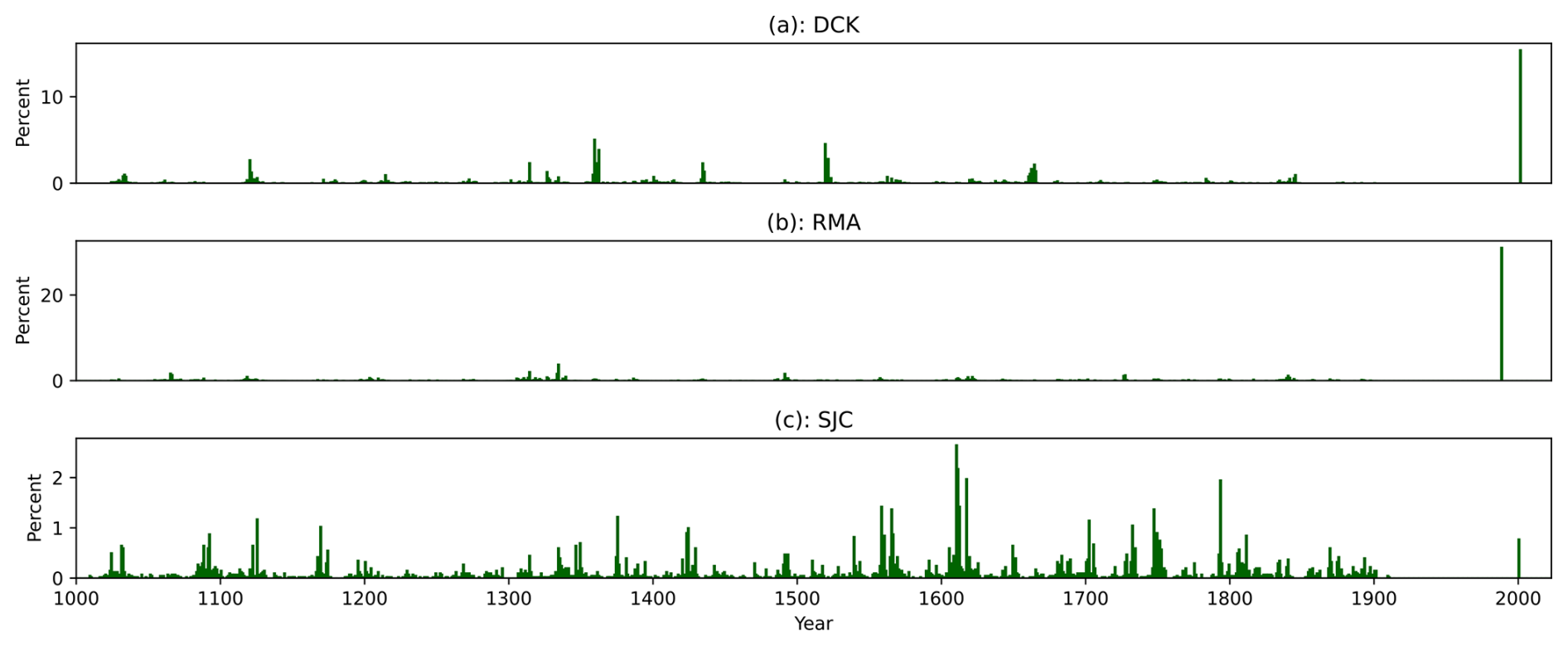
Figure 12 Wettest decades on record. Panel (a) shows the probability of a given ten year mean being the wettest (highest precipitation) decade since 1000 CE in Dodge City, Kansas. Years on the x-axis correspond to the end of the ten year period. Panel (b) shows the same for Red Mesa, Arizona. Panel (c) shows the same for Sonora Junction, California.

Our results also reinforce the unique nature of the late twentieth-century pluvial identified and discussed in Cook et al. (2025). There is a 15 % chance that 1992–2001 was the wettest ten-year period on record in DCK (Fig. 12a), and a 31 % chance that 1979–1988 was the wettest decade in RMA (Fig. 12b). No one decade stands out as the wettest in SJC, although it appears likely that the wettest ten-year stretch occcured in the early seventeenth century (Fig. 12c).

4 Discussion and Conclusions

The reconstruction method we present is interpretable, easily updated with new information, and provides full posteriors that incorporate multiple sources of uncertainty. However, it (like all statistical and machine learning methods) is contingent on the assumption that any differences between the training and test data are reflected in the model: that is, any dissimilarities between 1950–2023 and pre-1950 climate can be captured by removing a forced response that scales with global mean temperature (Eq. 3). This assumption may not hold in all years. For example, the extreme low 1934 Dust Bowl precipitation anomaly in Dodge City, Kansas was also accompanied by a record-shattering heat wave (red star, Fig. 13).

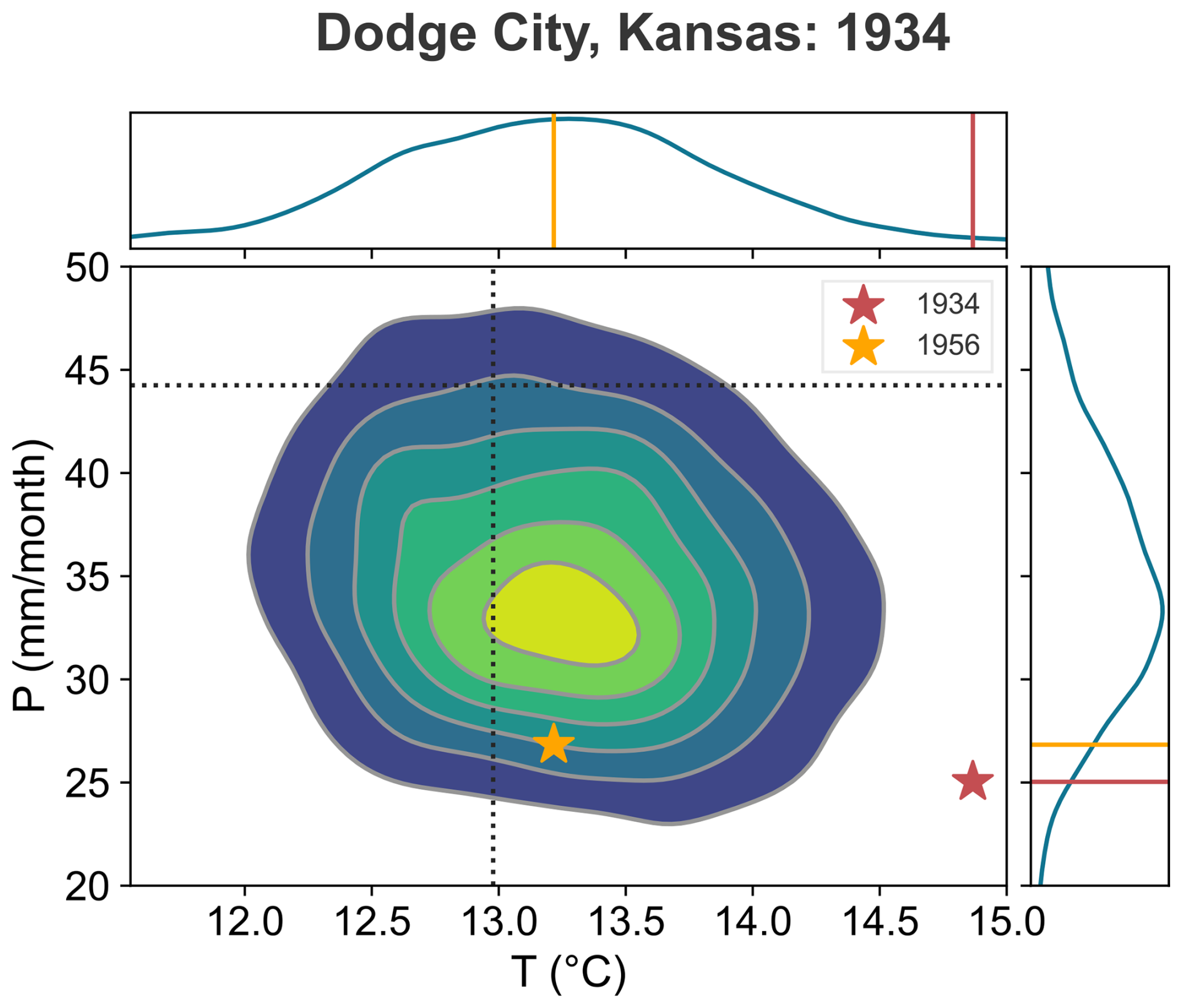
Figure 13 1934 was an exceptionally hot drought in Dodge City. Shown is the joint posterior PDF for reconstructed annual (September–August) DCK temperature and precipitation in 1934 (contour lines). Marginal PDFs are shown on the top (for T) and right (for P). Annual mean climatologies are shown as dashed lines. Instrumental annual mean temperature and precipitation for 1934 is shown as a yellow star. Instrumental T and P for 1956 is shown as a yellow star. Red/yellow lines on the marginal PDFs indicate 1934/1956 T (top) and P (right).

But over the training period (1950–2005), the DCK region simply did not experience hot droughts of this magnitude. In the latter half of the twentieth century, most anomalously low values of D in this region were associated with precipitation deficits. For example, the 1956 drought was associated with extremely low summertime precipitation (roughly similar to 1934) but the average summertime temperature, while still well above normal, was 1.67 °C colder than 1934 (yellow star, Fig. 13.

In fact, despite rising temperatures in all three regions, none of them show a sustained decrease in D. This suggests that, at least over the training period 1950–2005, summer season PDSI as recorded by tree rings is relatively insensitive to temperature. As a result, a model trained on the late 20th and early 21st century will fail to capture combined heat and drought extremes such as the conditions observed in 1934.

Further updates to the model itself are both possible and simple to incorporate. Here, we have presented a simple model that reconstructs joint probability distributions for temperature and precipitation from tree ring-based estimates of the Palmer Drought Severity Index D. Our method is fully Bayesian, which means our estimates can be easily updated in light of new information. It also means that the model can be easily extended to reflect more complexity or incorporate new sources of uncertainty. For example, there are several ways in which the simple modeling choices we make may be inadequate at capturing real-world phenomena. First, we use a simple AR(1) multivariate linear model for the reconstructed growing-season PDSI, in which D in a given year depends simply and linearly on T, P, and D in the previous year. We also assume that the meteorology $M=(T,P)$ is multivariate normal, with correlations between temperature and precipitation in different months and between each other in the same month. This neglects more complex possible covariance structures, including temporal structure that might give rise to multidecadal variability. Similarly, we treat the global mean temperature G over the past millennium as normally distributed, which precludes the identification of more complex patterns of temporal noise.

These potential defects may be addressed in further work by a combination of more data and more sophisticated models. For example, internal variability in M might be modeled by an autoregressive or Gaussian process with multiple spatial and temporal kernels to capture covariances between T and P over multiple temporal and spatial scales. Conversely, independent or quasi-independent reconstructions of global mean temperature may be used for G1000 instead of treating it as a model parameter.

Despite these limitations, our method proves surprisingly adept at reconstructing conditions over the validation period, especially for precipitation. The Bayesian inverse model struggles to capture regional temperatures for the simple reason that regional JJA D over the training period is far more sensitive to rainfall than temperature. One notable advantage of this method is its ability to provide a joint posterior probability distribution, capturing the combinations of temperature and precipitation that may result in any given D.