the Creative Commons Attribution 4.0 License.
the Creative Commons Attribution 4.0 License.
 | 30 Nov 2018
Estimates of climate system properties incorporating recent climate change
Alex G. Libardoni
Andrei P. Sokolov
Erwan Monier
Historical time series of surface temperature and ocean heat content changes are commonly used metrics to diagnose climate change and estimate properties of the climate system. We show that recent trends, namely the slowing of surface temperature rise at the beginning of the 21st century and the acceleration of heat stored in the deep ocean, have a substantial impact on these estimates. Using the Massachusetts Institute of Technology Earth System Model (MESM), we vary three model parameters that influence the behavior of the climate system: effective climate sensitivity (ECS), the effective ocean diffusivity of heat anomalies by all mixing processes (Kv), and the net anthropogenic aerosol forcing scaling factor. Each model run is compared to observed changes in decadal mean surface temperature anomalies and the trend in global mean ocean heat content change to derive a joint probability distribution function for the model parameters. Marginal distributions for individual parameters are found by integrating over the other two parameters. To investigate how the inclusion of recent temperature changes affects our estimates, we systematically include additional data by choosing periods that end in 1990, 2000, and 2010. We find that estimates of ECS increase in response to rising global surface temperatures when data beyond 1990 are included, but due to the slowdown of surface temperature rise in the early 21st century, estimates when using data up to 2000 are greater than when data up to 2010 are used. We also show that estimates of Kv increase in response to the acceleration of heat stored in the ocean as data beyond 1990 are included. Further, we highlight how including spatial patterns of surface temperature change modifies the estimates. We show that including latitudinal structure in the climate change signal impacts properties with spatial dependence, namely the aerosol forcing pattern, more than properties defined for the global mean, climate sensitivity, and ocean diffusivity.
- Article
(9294 KB) - Full-text XML
- BibTeX
- EndNote


Scientists, policy makers, and the general public are concerned with how surface temperature will change in the coming decades and further into the future. These changes depend on many aspects of the climate system. Among them are climate sensitivity and the rate at which heat is mixed into the deep ocean. Equilibrium climate sensitivity (ECS) represents the global mean surface temperature change that would be realized due to a doubling of CO2 concentrations after equilibrium is reached. A shorter-term measure of climate sensitivity to greenhouse gas forcing is transient climate response (TCR), defined as the global mean surface temperature change at the time of CO2 doubling in response to CO2 concentrations increasing at a rate of 1 % per year (Bindoff et al., 2013). Due to the climate system not being in equilibrium, interactions between the surface and the ocean lead to an exchange of energy. In such a scenario, TCR is a function of both the climate sensitivity and ocean circulation and mixing (Andrews and Allen, 2008; Sokolov et al., 2003).
The value of climate sensitivity is uncertain but the processes and feedbacks which set it must be accurately modeled to reliably predict the future. To this end, a number of studies have used Earth System Models of Intermediate Complexity (EMICs) to estimate probability distribution functions (PDFs) for the values of these climate system properties, in particular ECS, ocean diffusivity, and an estimate of the anthropogenic aerosol forcing (Aldrin et al., 2012; Forest et al., 2002, 2008; Knutti et al., 2003; Libardoni and Forest, 2013; Olson et al., 2012; Tomassini et al., 2007). In these studies, EMICs are run for many combinations of the model parameters that set the climate system properties. Model output is then compared to historical temperature change to determine which model states best match the past.
Time series of surface temperature and ocean heat content are commonly used temperature diagnostics in the evaluation of model performance because they rule out different combinations of the parameters for being inconsistent with the observed climate record (Urban and Keller, 2009). This helps to narrow the estimates of the parameters because only certain combinations lead to accurate representations of the past. Observations in the early 21st century showed that the rate of increase in global mean surface temperature slowed despite the continued rise of global CO2 concentrations (Trenberth and Fasullo, 2013). This slowdown was the source of debate as to whether climate change was a significant threat and led scientists to search for the reasons why temperatures did not rise as much as expected. Cowtan and Way (2014) and Karl et al. (2015) argue that the slowdown was merely an artifact of the global observing system and the result of incomplete coverage in the polar regions where temperatures increase most rapidly. The slowdown was also attributed to changes in the radiative forcing. In particular, it is argued that the forcing due to the Sun, anthropogenic aerosols, and volcanoes all contributed to reduce global mean temperature in the 2000s (Huber and Knutti, 2014; Schmidt et al., 2014). Natural variability in the ocean has also been noted as a potential cause of the slowdown (Huber and Knutti, 2014; Meehl et al., 2011; Schmidt et al., 2014). In particular, Meehl et al. (2011) show that in a fully coupled, three-dimensional climate model, periods of little to no rise in surface temperatures are associated with enhanced mixing of heat below 300 m in the ocean. This finding is supported by recent observations showing that heat is accumulating more rapidly in the deep ocean (Gleckler et al., 2016; Levitus et al., 2012). Any good model simulation should be able to capture these features of the past.
In this study, we first seek to improve the methods used in previous work (Forest et al., 2008; Libardoni and Forest, 2013; Libardoni et al., 2018a). Until now, ensembles from different versions of the MIT Integrated Global Systems Model (Sokolov et al., 2005) have been used to vary model parameters for ECS, ocean diffusivity, and the net anthropogenic aerosol scaling factor using a gridded sampling strategy. To derive PDFs for the model parameters, metrics of model performance at parameter settings in between those where the model was run are estimated using two-dimensional interpolation algorithms. These algorithms are restricted to gridded samples and at times have led to PDFs that are not smooth. We propose and implement a new method where spline interpolations are replaced with a radial basis function interpolation algorithm. We show that the new method leads to PDFs that are both true to the data and smooth by using the 1800-member ensemble of the MIT Earth System Model (Sokolov et al., 2018) described in Libardoni et al. (2018a) to derive PDFs for the three model parameters.
Using the updated methodology and the 1800 MESM runs, we answer the following questions: (1) how does the inclusion of more recent data change the PDFs of model parameters? And (2) what do we learn by including spatial information in the surface diagnostic? The inclusion of recent temperature trends can have a significant impact on the estimates of climate system properties (Johansson et al., 2015; Urban et al., 2014). The temperature pattern that the model output is compared against becomes more detailed as data are added and leads to the rejection of more model runs as being inconsistent with the observed records. This generally leads to both a shift in the estimation of a given property and a reduction in the uncertainty in the estimate. Urban et al. (2014) also showed that the ability to distinguish between different states of the climate increases as the length of the model diagnostic increases. Similar to Johansson et al. (2015), we identify the influence of including more recent data by systematically adding data to the time series.
Second, we show how including spatial variability in the surface temperature diagnostic can influence the parameter distributions. In almost all parameter estimation studies, global mean ocean heat content is used as one metric to evaluate model performance and is paired with a surface temperature diagnostic to further test the model runs. Typically, groups use time series of either global mean surface temperature (Knutti and Tomassini, 2008; Knutti et al., 2002; Olson et al., 2012; Tomassini et al., 2007; Urban and Keller, 2009) or hemispheric mean surface temperatures (Aldrin et al., 2012; Andronova and Schlesinger, 2001; Meinshausen et al., 2009; Skeie et al., 2014) as the surface diagnostic. Given the latitudinal resolution of MESM, we can estimate zonal temperature patterns beyond global and hemispheric means. In particular, we use a surface temperature diagnostic that consists of four equal-area zonal bands, allowing the observed amplification of polar warming to be included in the evaluation of model performance. We show the impact of the spatial structure of the surface diagnostic by deriving PDFs using global mean, hemispheric mean, and four zonal mean temperature diagnostics.
In Sect. 2, we introduce the general method for estimating the probability distributions for the model parameters, describe the temperature diagnostics, and introduce an interpolation method for the likelihood function using radial basis functions. We present our main findings in Sect. 3 and finish with a summary and conclusions in Sect. 4.
As outlined in Sect. 1, we propose and implement a number of methodological changes designed to improve our estimates of the probability distributions of the model parameters. Here, we first provide a general overview of our method for deriving the distributions, including a description of the model diagnostics and their derivation. We follow with a discussion of the new methods used in this study and how they are applied to deriving the new distributions.
Following a standard methodology (Forest et al., 2006, 2008; Libardoni and Forest, 2011; Olson et al., 2012), we derive probability distributions for the model parameters. In this method, EMICs are used to run simulations of historical climate change. By comparing model output to observations, the likelihood that a run with a given set of parameters represents the climate system is determined by how well it simulates the past climate. In this study, we use the MESM, which includes three adjustable parameters that set properties that strongly influence the behavior of the climate system. These model parameters are the cloud feedback parameter, which sets the effective climate sensitivity (ECS), the effective ocean diffusivity of heat anomalies by all mixing processes (Kv), and the net anthropogenic aerosol forcing scaling factor (Faer). We identify each run by a unique combination of the model parameters, θ, where θ = (ECS, Kv, Faer). In this study, we take the 1800-member ensemble described in Libardoni et al. (2018a), spanning a wide range of θs, as our model output.
We evaluate model performance by comparing each model run to two temperature diagnostics. The first diagnostic is the time series of decadal mean surface temperature anomalies in four equal-area zonal bands spanning 0–30 and 30–90 ∘ latitude in each hemisphere. Temperature anomalies are calculated with respect to a chosen base period. The second diagnostic is the linear trend in global mean ocean heat content in the 0–2000 m layer. For each diagnostic, we now describe the data used for observations and the methods to derive the diagnostics from the observations.
For surface observations, we use datasets from four different research centers. The datasets we use include the median of the 100-member HadCRUT4 ensemble from the Hadley Centre Climatic Research Unit (Morice et al., 2012), the Merged Land-Ocean Temperature (MLOST) dataset from NOAA (Vose et al., 2012), the Berkeley Earth Surface Temperature (BEST) dataset (Rohde et al., 2013), and the GISTEMP dataset with 250 km smoothing (GISTEMP250) from the NASA Goddard Institute for Space Studies (Hansen et al., 2010). All datasets are given as monthly temperature anomalies on a 5×5 ∘ latitude–longitude grid. The datasets use similar station data over land but differ on which sea surface temperature (SST) dataset is used for the ocean. In particular, the HadCRUT4 and BEST datasets use the Hadley Centre SST (HadSST) dataset (Kennedy et al., 2011a, b) and the MLOST and GISTEMP250 datasets use the Extended Reconstruction Sea Surface Temperature (ERSST) dataset (Huang et al., 2015). Furthermore, the base period used to calculate temperature anomalies differs among the datasets. A 1951–1980 base period is used for BEST and GISTEMP250, a 1961–1990 base period is used for HadCRUT4, and a 1971–2000 base period is used for MLOST. Lastly, the research centers differ in how they fill in sparse data regions.
We derive the surface temperature diagnostic by temporally and spatially averaging the gridded data. In the following calculation, we assume uncertainty in the observations is zero, relying on using multiple datasets to account for uncertainty in the observed record. Due to data scarcity and missing values in some regions, we set threshold criteria for each spatial and temporal average in the derivation. First, the annual mean for each 5×5 ∘ grid box is calculated, provided that at least 8 months of the year have non-missing data. From these annual averages, decadal mean time series are calculated for both the period being used in the diagnostic and the chosen climatological base period. For these calculations, we require at least 8 years of defined data for a decadal mean to be defined. We also extract from the annual mean time series a data mask indicating where observations are present or missing. We use this mask on the model output to match the coverage of the observations.
Once the data mask and decadal mean time series are calculated, each time series is zonally averaged on the 5 ∘ grid. The zonal mean is marked as undefined if there is less than 20 % longitudinal coverage in a given latitude band. We calculate temperature anomalies for each zonal band by subtracting the mean of the climatological time series for the given band from each decade of the comparison period time series. The resulting time series of decadal mean, 5 ∘ resolution temperature anomalies are then averaged into the four equal-area zones. When aggregating to larger areas, the mean is calculated as the area-weighted average of the zonal bands contained within the larger zone.
For ocean heat content observations, we use the estimated global mean ocean heat content in the 0–2000 m layer from Levitus et al. (2012). This dataset replaces the Levitus et al. (2005) 0–3000 m global mean dataset because the latter ends in 1998 and we aim to extend the diagnostic into the 21st century. Data are presented as heat content anomalies in 5-year running means, starting with the 1955–1959 pentad and ending in the 2011–2015 pentad. Also included in the Levitus et al. (2012) data is a time series of the standard error of the pentadal mean estimate for the global mean heat content. The procedure for deriving the standard error estimates is described in the study's Supplement and is based on the observational error estimates of the 1 ∘ gridded data.
For a given diagnostic period, we calculate the linear trend in the global mean ocean heat content as the slope of the best-fit linear regression line. In the calculation of the regression line, all deviations from the mean are assigned a weight inversely proportional to the square of the standard error from the Levitus et al. (2012) data at that point in the time series. For example, the standard deviation of y from the mean,
is modified by multiplying each term in the summation by its weight, giving the weighted standard deviation of y from the mean of
where wi is the weight assigned to each point yi based off of the observational error estimate. All summation terms in the regression are replaced by the corresponding weighted version. By doing so, the regression is weighed more towards portions of the time series for which the standard error of the observations is small. Because observational errors decrease in latter years, more recent observations have a stronger influence on the trend estimate.
Each model run is compared to the model diagnostics and evaluated through the use of a goodness-of-fit statistic,
where x(θ) and y are vectors of model output for a given set of model parameters and observed data, respectively, and is the inverse of the noise-covariance matrix. The noise-covariance matrix is an estimate of the internal variability of the climate system and represents the temperature patterns we would expect in the absence of external forcings. We estimate the noise-covariance matrix by drawing samples of the temperature diagnostics from the control run of fully coupled general circulation climate models and calculating the covariance across the samples. Prior to this study, separate models were used for the surface and ocean diagnostics, potentially yielding inconsistent variability estimates. We eliminate that issue by using the Community Climate System Model, version 4 (Gent et al., 2011) to estimate the natural variability for both the surface and ocean diagnostics. In its simplest form, the r2 statistic is the weighted sum of squares residual between the model simulation and the observed pattern. Multiplying x(θ)–y by the noise-covariance matrix rotates the patterns into the coordinate space of the natural variability and scales the differences such that r2 is the sum of independent normals. The noise-covariance matrix is thus a pre-whitener of the residuals.
From the r2 field, we calculate
the difference between r2 at an arbitrary point and the minimum r2 value in the domain. The run with minimum r2 represents the model run with parameters θ that best matches the observed record. Δr2 gives a measure of how much an arbitrary run differs from the model run that produces the best fit to the observations. Whereas regions with large Δr2 indicate θs that do not simulate the particular diagnostic well, regions with small Δr2 indicate θs that simulate the particular diagnostic comparably to the minimum. Regions of high (low) Δr2 can (cannot) be rejected for being inconsistent with the observed climate record.
Because of the pre-whitening by the noise-covariance matrix, Δr2 is known to follow an F distribution (see Forest et al., 2001, for a complete derivation and discussion). Knowing the distribution of Δr2 provides the link between the goodness-of-fit statistics and the final PDFs. Through this connection, we convert r2 to probability distribution functions for the model parameters using the likelihood function based on an F distribution described in Libardoni and Forest (2011) and modified by Lewis (2013). Through an application of Bayes' theorem (Bayes, 1763), we combine the likelihoods from each diagnostic and a prior on the model parameters to estimate the joint PDF. We apply the expert prior derived in Webster and Sokolov (2000) to ECS and uniform priors to Kv and Faer. Probability distributions for individual parameters are calculated by integrating the joint PDF over the other two parameter dimensions.
Prior to calculating the likelihood function, we interpolate the goodness-of-fit statistics onto a finer grid in the parameter space. This interpolation fills in the gaps between θs where the model was run and increases the density of points within the domain. Forest et al. (2006) presented an interpolation method that was implemented in Libardoni and Forest (2011). The interpolation is first carried out on ECS– planes via a spline interpolation on all Faer levels to a finer mesh of points. A second set of spline interpolations at every ECS– point on the fine mesh then fills in the fine grid in the Faer dimension.
In this study, we implement an alternate interpolation method based off of radial basis functions (Powell, 1977). The RBF method approximates the value of a function based off of a set of node points where the functional value is known and is a variation of kriging that does not allow the data to inform the internal parameters of the algorithm. The function value at any point in the domain is calculated as the weighted sum of the value at all nearby node points. The weight assigned to each node is related to the radial distance between the location that is being interpolated to and the node. We view this method as an improvement because it is a three-dimensional method and does not require multiple steps. We will also show in Sect. 3.1 that this leads to a smoother interpolation surface.
For our implementation, we use the 1800 r2 values at the points θ where the model has been run as nodes. For node points, we have sampled ECS from 0.5 to 10.0 ∘C in increments of 0.5 ∘C, from 0 to 8 in increments of 1 ), and Faer from −1.75 to 0.5 W m−2 in increments of 0.25 W m−2. We interpolate the r2 values from the θs of the node points to the fine grid used in the spline interpolation method. In particular, we interpolate r2 values for ECS between 0.5 and 10.5 ∘C in increments of 0.1 ∘C, between 0 and 8 in increments of 0.1 , and Faer between −1.75 and 0.5 W m−2 in increments of 0.05 W m−2. For weights, we choose Gaussian basis functions, with the weight assigned to each node given by
where ϕ is the weight, d is the radial distance between the two points, and ϵ is a scaling parameter that determines how quickly the weight decreases with distance. Typically, RBFs are calculated in physical space, where the distance between points, d, is well defined. However, in this application, we need to apply the concept of distance in model parameter space. Because the spacing between nodes in each dimension of the parameter space is different, we normalize all distances by the range in a given parameter dimension. We recognize that this choice of normalization constant is arbitrary and in the future should be determined by a physical metric. Once normalized, we treat each parameter dimension as isometric, so that the distance between two points is represented by
where subscript i refers to the interpolated point, subscript n refers to the node points, and the normalization constants are 9.5 ∘C in ECS, 8 in , and 2.25 W m−2 in Faer. Because the distance between any two points in the parameter space is always the same, the choice of ϵ plays a critical role in determining the behavior of the algorithm. We demonstrate this by showing the weights for six different ϵ values as a function of normalized distance (Fig. 1). Small values of ϵ lead to a slow decay and large values of ϵ lead to a rapid decay of the weighting function. The choices of ϵ are described in Appendices A and B.
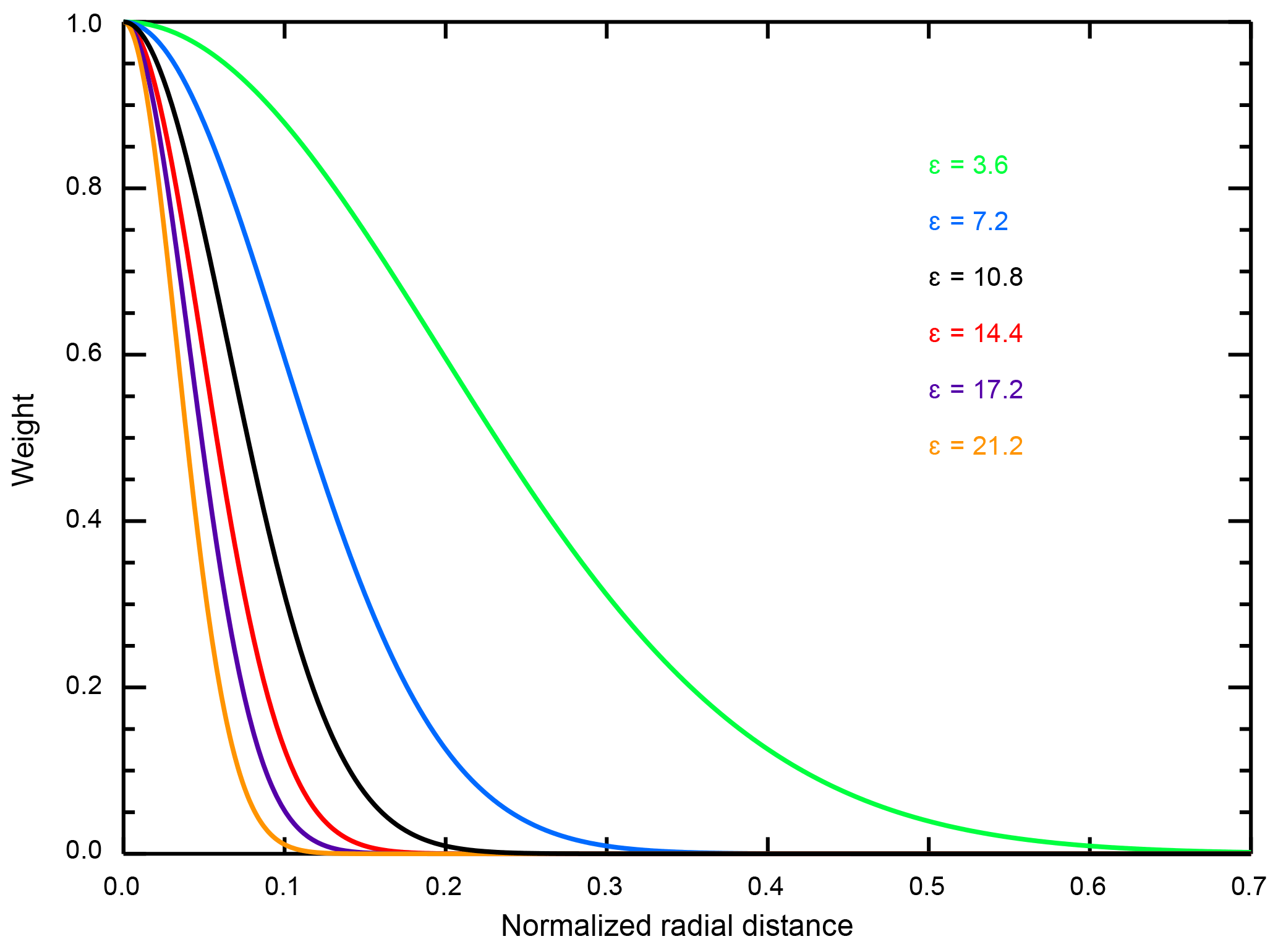
Figure 1Weight assigned to each node point as a function of radial distance in normalized parameter space. The decay is isometric in the parameter space and the same for all node points.
The weighting function is applied to each node point within the parameter space. One can imagine a sphere surrounding each of these points, with the weight assigned to that point decaying as a function of the distance from the center. All points within the parameter space are in regions where the spheres from multiple node points overlap. The interpolated value at any point is the weighted sum of the node values associated with the overlapping spheres. Thus, we calculate the r2 value at any point in the domain as
where the sum is over all N=1800 node values. When calculating the sum, all 1800 node values are considered, but the weights from those far away in parameter space are close to zero and do not contribute to the sum.
In summary, we have made a number of changes and updates to the methodology. (i) To account for a change in observational dataset, we have modified the ocean diagnostic to be estimated from the 0–2000 m layer, as opposed to the 0–3000 m layer. (ii) We now estimate the natural variability from a common model, as opposed to using different models for the surface and ocean diagnostics. (iii) We implement a new interpolation scheme where radial basis functions are used to interpolate goodness-of-fit statistics from the coarse grid of model runs to the fine grid used to derive the joint probability distribution functions.
Using the updated methodology, we show how temporal and spatial information impacts the PDFs of the model parameters. We address the temporal component by adding more recent data to the model diagnostics in one of two ways. First, we extend the diagnostics by fixing the starting date while shifting the end date forward in time. To maximize the amount of data that we use in the surface diagnostic while also ensuring good observational data coverage, we take decadal mean temperature anomalies with respect to the 1906–1995 base period starting in 1941. We then shift the end date from 1990 to 2000 to 2010 to change the diagnostics from 5 to 6 to 7 decades, respectively. For the ocean diagnostic, we choose 1955 as the starting date of the first pentad to correspond to the beginning of the observational dataset. Similar to the surface diagnostic, we increase the length of the ocean diagnostic by changing the end date of the last pentad from 1990 to 2000 to 2010.
In a second test, we fix the length of the diagnostics while shifting the end date forward in time. This maintains a 5-decade diagnostic for the surface diagnostic by shifting the 50-year window from 1941–1990 to 1951–2000 to 1961–2010 and a 35-year ocean diagnostic by shifting the period we use to estimate the linear trend from 1955–1990 to 1965–2000 to 1975–2010. By deriving PDFs with each pair of diagnostics corresponding to a given end date, we determine the impact of recent temperature trends on the parameter distributions in both the extension and sliding window cases.
In a third test, we derive PDFs with different structures for the surface diagnostic. In these new diagnostics, we maintain the decadal mean temporal structure but reduce the dimensionality of the spatial structure by replacing the four zonal bands with global mean or hemispheric mean temperatures. In the former case, we have a one-dimensional spatial structure, and in the latter a two-dimensional structure.
We present our findings as follows. In Sect. 3.1 we (i) show the difference in the ocean diagnostic due to changing to the 0–2000 m data, (ii) provide justification for using the RBF interpolation method, and (iii) present the impact of the methodological changes described in Sect. 2 on the parameter distributions. In Sect. 3.2, we (i) analyze how the model diagnostics change due to the inclusion of more recent data and (ii) assess how those changes impact the distributions. In Sect. 3.3, we show how including spatial patterns of surface temperature change impact the distributions.
3.1 Methodological changes
We first identify the difference in the ocean diagnostic derived from the 0–3000 and 0–2000 m layers for the common period of 1955–1996 (Fig. 2). This period is chosen to coincide with the ocean diagnostic in Libardoni and Forest (2013) and allows for a direct comparison of distributions presented later in this section. We observe a stronger warming trend of 3.6±0.50 ZJ yr−1 in the 0–2000 m layer compared to the estimate of 2.7±0.39 ZJ yr−1 in the 0–3000 m layer, suggesting that the rate of heat penetration into the deep ocean decreases with depth.
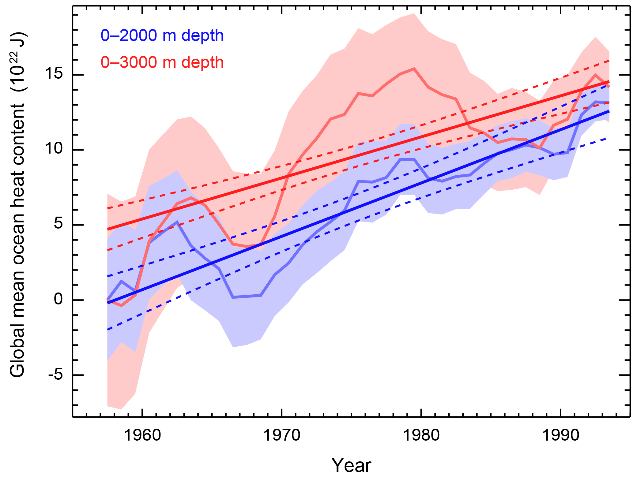
Figure 2Global mean ocean heat content for the 0–3000 m layer (Levitus et al., 2005) and 0–2000 m layer (Levitus et al., 2012). Shading indicates twice the standard error on either side of the estimate. Standard error estimates are included with the time series from the respective datasets. Dashed lines represent the 95 % confidence interval for the trend line derived from the data and its uncertainty estimates.
Second, we demonstrate the impact of switching to the RBF algorithm. For one of our surface temperature diagnostics, we interpolate the r2 values using each of the six ϵ values presented in Sect. 2. We show the resulting r2 patterns and compare them against the surface derived using the Forest et al. (2006) spline interpolation method and the original pattern (Fig. 3). We observe that the old method is very successful at matching the r2 values at points where they were run (Fig. 3b). However, the surfaces are not always smooth and in some instances the location of the minimum value of r2 shifts to a new, nearby location in the interpolated space.
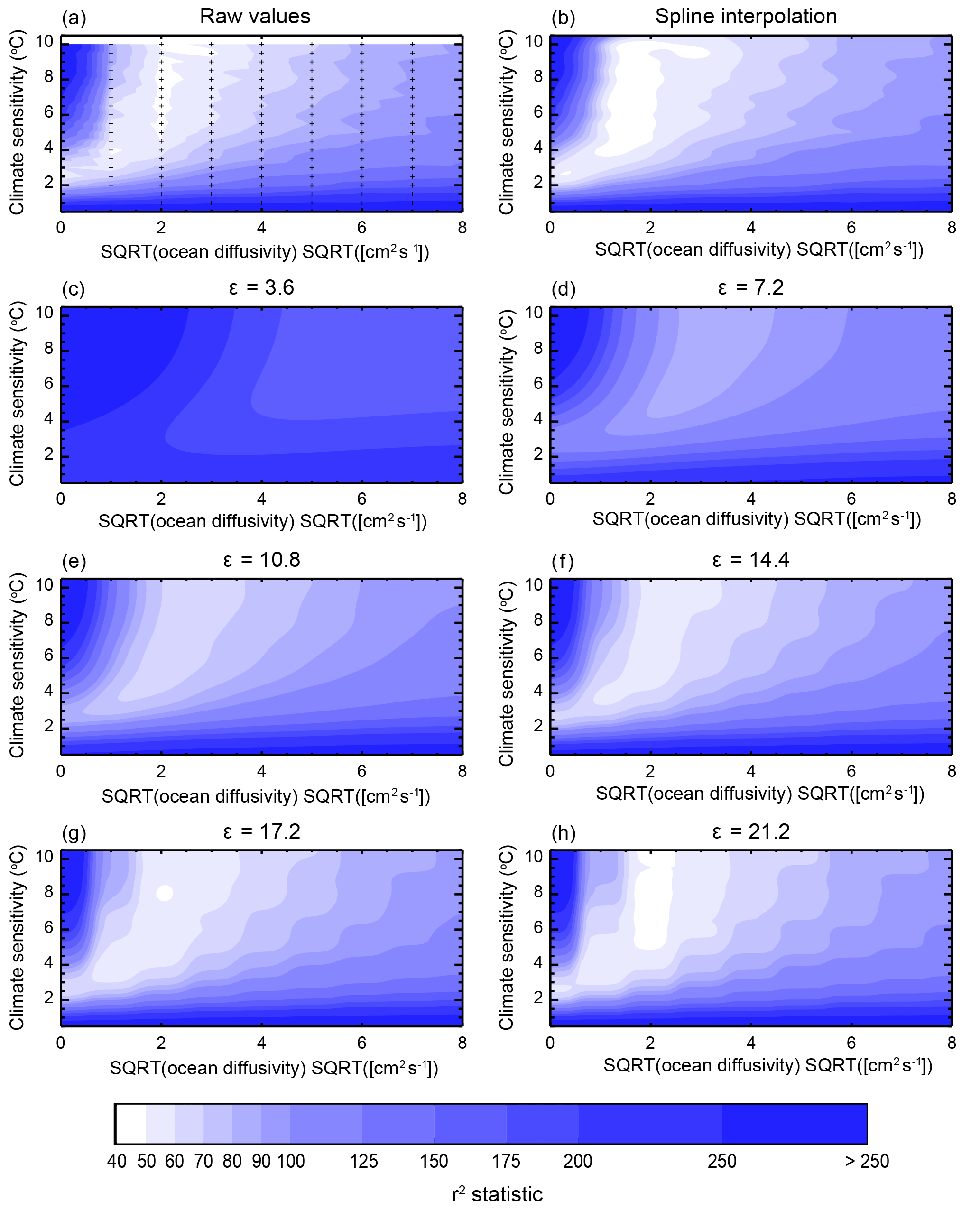
Figure 3Example of the differences between the algorithms to interpolate goodness-of-fit statistics from the coarse grid of model runs to the finer grid used for the derivation of parameter distributions. Calculated r2 values (a) are shown along with the interpolated values using the algorithm from Libardoni and Forest (2011) (b) and the radial basis function interpolation with six different values of ϵ (c–h). Node points (+) are indicated in (a), while the interpolated grid has been omitted for clarity (b–h).
We aim to improve upon the shortcomings of the old interpolation method by identifying ϵ so that not only is the spatial pattern of r2 maintained, but the resulting response surface is also smooth. We observe smoother interpolated surfaces for lower values of ϵ because of the relationship between ϵ and the radius of influence of each node point (Fig. 3c–h). Because we do not require the interpolated values to pass exactly through the node points, the smoothness comes at the expense of increasing the interpolation error at the node points. Unlike the old interpolation method, the errors at node points do not lead to a change in the rank order of r2 values at the node points, however. The location of the minimum remains the same, as well as all subsequent comparisons.
We also observe a reduction in the range of r2 values within the domain. The reduction occurs because regions where r2 is originally low are now influenced by areas further away in the parameter space where r2 is high, and vice versa. This is true of the algorithm in general, with the errors at each node point and the reduction of the range diminishing as ϵ increases and the radius of influence of each node point decreases. However, as ϵ increases and the radius of influence for a given node decreases, the response surface becomes less smooth. Thus, there is a tradeoff, in that decreasing the interpolation error at node points leads to a decrease in the smoothness of the surface. Small ϵs provide the desired smoothness, while large ϵs provide the truest fit to the actual values at the node points. This indicates that intermediate values of ϵ (e.g., 10.8 or 14.4) are appropriate.
Thus far, we have only investigated the impact of ϵ on the fit of the interpolated r2 values to the raw values. As outlined in Sect. 2, inference on the model parameters is based on Δr2, the difference between r2 at an arbitrary point in the parameter space and the minimum within the domain. Plotting the Δr2 field as a function of ϵ confirms our assessment that intermediate values of ϵ lead to the best fit to the raw values (Fig. 4). Both ϵ=10.8 and ϵ=14.4 fit the raw Δr2 values quite well as the inflation of low r2 values is normalized by the subtraction of the minimum value (which is also interpolated to a greater value). However, for ϵ = 14.4, the region of best fit (Δr2 less than 10) is larger than the raw values and there are regions where the interpolated surface is not as smooth as when ϵ=10.8. In some situations, this lack of smoothness leads to PDFs that are also not smooth and display bumps at values for the parameter settings of the node points (not shown). For these reasons, we choose ϵ=10.8 for our analysis.

Figure 4As in Fig. 3, except for Δr2, the difference between r2 at a given point and the minimum r2 value in the domain. This represents the difference between r2 at an arbitrary point and that of the best fit of the model to the observations.
To further test our choice of ϵ, we perform an out-of-sample test on 300 runs of the MESM that were not included in the 1800 member ensemble used in this study. The parameter settings for the out-of-sample runs were the result of two separate 150-member Latin hypercube samples (McKay et al., 1979) and did not correspond to the settings of any of the node points. For each run, we calculate Δr2 for the surface diagnostic matching the one used in Figs. 3 and 4 and compare those against the values calculated using the RBF interpolation method with ϵ=10.8 and the 1800 runs as nodes (Fig. 5).
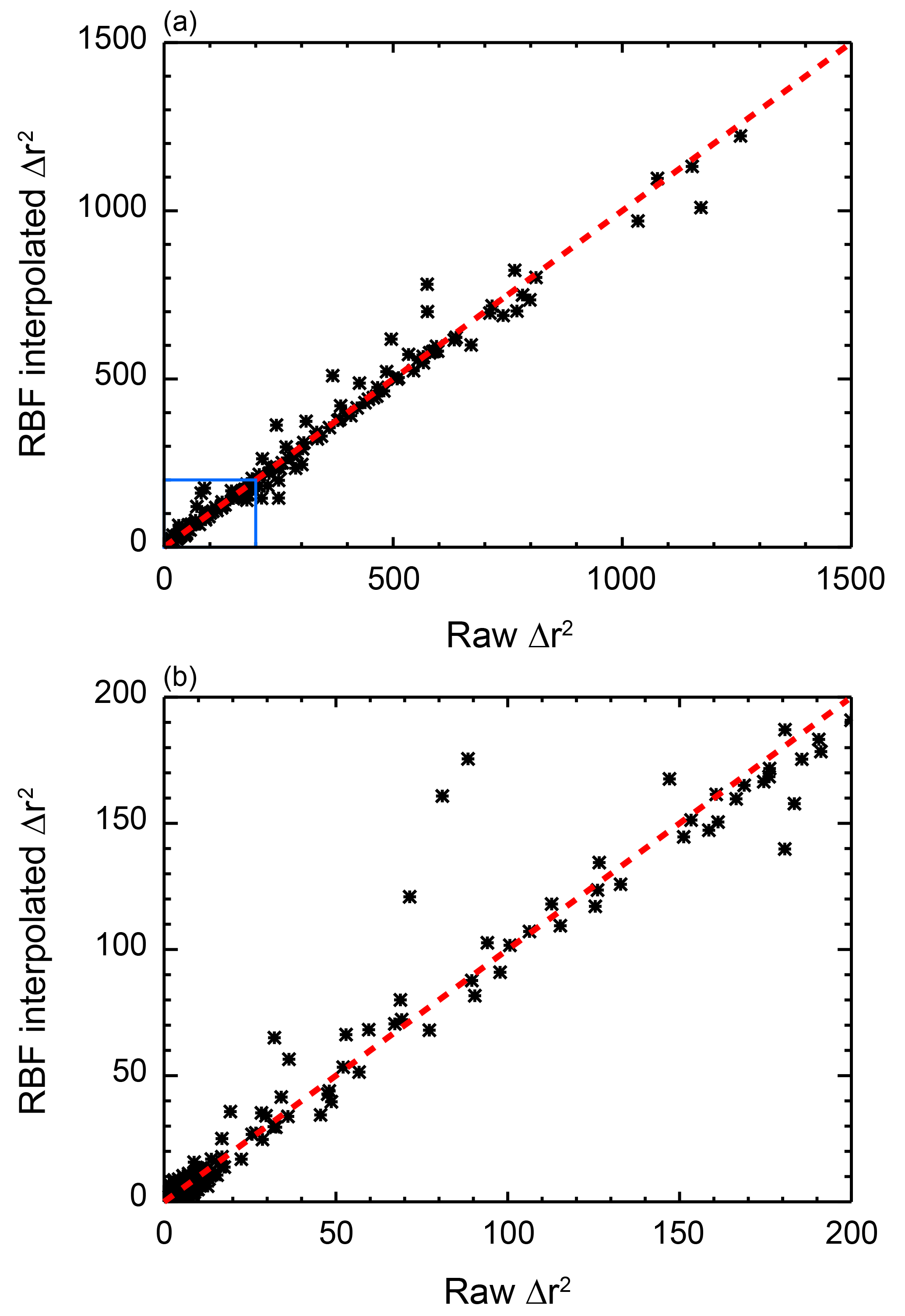
Figure 5Comparison of Δr2 values calculated from out-of-sample model runs and those calculated using the RBF interpolation method. (a) All 300 runs. (b) All runs with Δr2 less than 200. The one-to-one line is plotted for reference (red, dashed line).
With a few exceptions, we see good agreement between Δr2 calculated from the model output and Δr2 estimated from the RBF algorithm. The biggest discrepancies are typically found for Δr2 values greater than 50, where the likelihood function for the diagnostic approaches 0. We also note that the differences are small in regions of the parameter space where the likelihood function approaches its maximum, namely for small Δr2. Lastly, we find an almost equal number of runs where the difference between the value calculated from the model output and the value estimated from the RBF method is greater than zero and where the difference is less than zero, indicating no substantial bias in the RBF algorithm. Because we see good agreement of the RBF interpolated surface with the out-of-sample test runs and observe a smooth response surface with a good fit to the data (Figs. 3 and 4), we argue that choosing ϵ=10.8 is appropriate.
To test the impact of the methodological changes, we start from a previously published probability distribution and apply the changes one at a time. For a reference point, we start with the PDF from Libardoni et al. (2018a) derived using the HadCRUT3 surface temperature dataset (Brohan et al., 2006) and the likelihood function presented earlier in Sect. 2. The changes we implement are to (i) change the ocean diagnostic from the 0–3000 m layer to the 0–2000 m layer, (ii) replace the interpolation method of Forest et al. (2006) with the RBF interpolation method, and (iii) change from using natural variability estimates from different control run models for the surface and ocean diagnostics to a common model for both estimates. To better illuminate the changes, we derive an additional PDF changing both the control run model and the interpolation method simultaneously. We summarize the resulting distributions in Fig. 6.
When changing the ocean diagnostic from the 0–3000 m layer to the 0–2000 m layer, we observe the largest change as a shift towards higher Kv. As measured by the 90 % credible interval for the marginal distribution of , our estimate increases from 0.29–1.90 to 0.81–3.22 . We also note that the wider interval indicates a weaker constraint on the estimate of Kv. In the MESM, Kv controls how fast heat is mixed into the deep ocean. Thus, we trace the shift towards higher Kv to the stronger heating rate in the ocean diagnostic due to estimating the trend from the 0–2000 m data (Fig. 2). We observe a small shift towards higher ECS and almost no change in estimates of Faer.
For the second change, we explore the implementation of the RBF interpolation algorithm. In Fig. 6, we observe that the parameter distributions are indeed smoother when the RBF method is used. This is particularly evident in the climate sensitivity distributions. We also note changes to the constraints on model parameters. In general, we see a flattening of the center of the distributions, as measured by the interquartile range (IQR). In particular, the IQR for increases from 0.59 to 0.71 (ranges of 0.71–1.3 to 0.86–1.57 ) and for from 0.07 to 0.11 W m−2 (−0.25–−0.18 to −0.32–−0.21 W m−2) when comparing the reference PDF using the old interpolation method to the PDF estimated using the RBF method. This increase is consistent with our previous discussion that the RBF method tends to adjust low r2 values upwards and high r2 values downwards. In this situation, the maximum likelihood region of the joint PDF, where r2 is a minimum, impacts all points within its radius of influence.
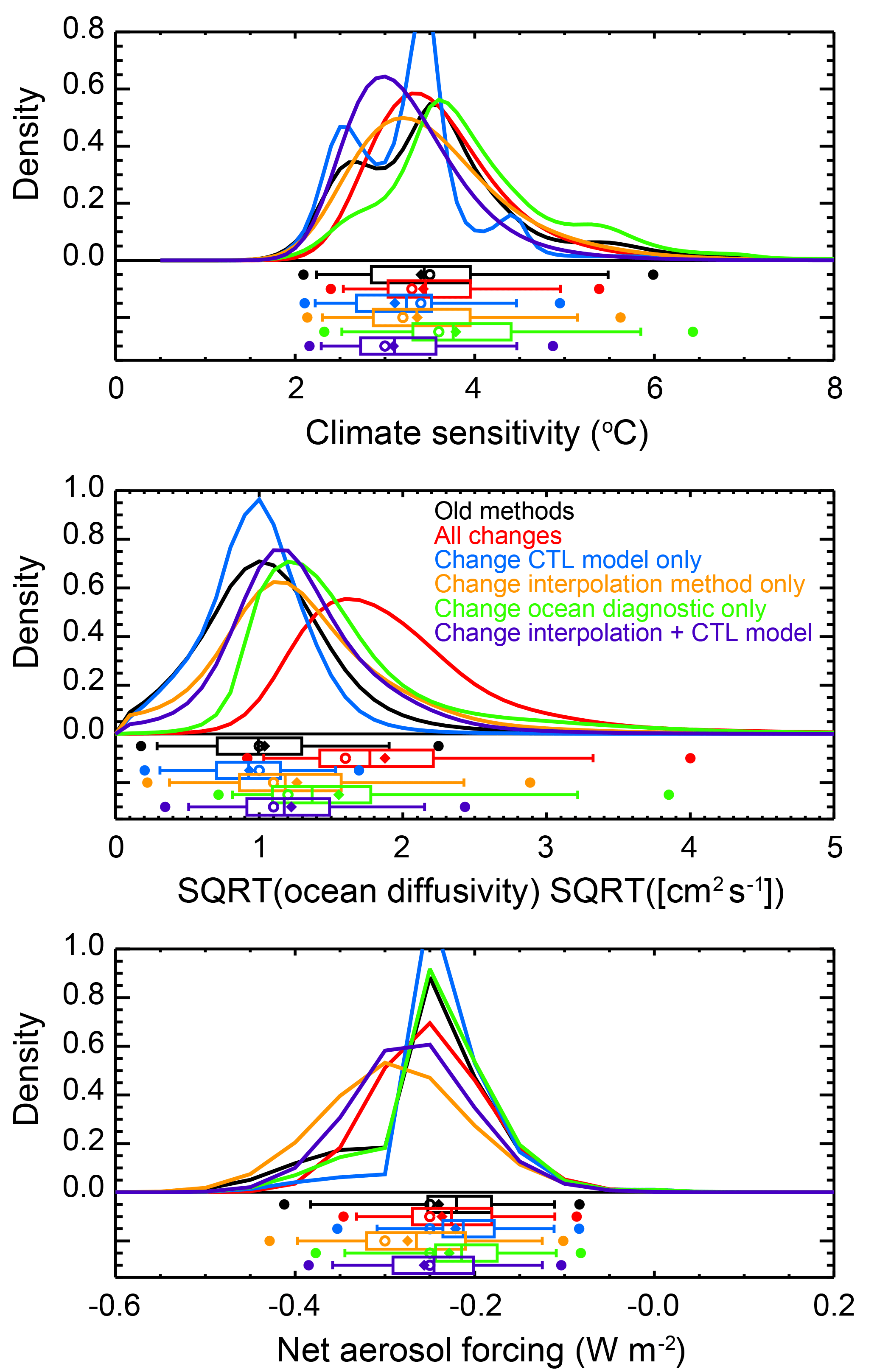
Figure 6Marginal probability distribution functions for (a) ECS, (b) , and (c) Faer derived with changes in methodology. A comparison between the HadCRUT3 distribution derived in Libardoni et al. (2018a) (black) with those derived using all changes outlined in the text (red) and individual changes to the control run used to estimate natural variability (blue), the ocean diagnostic (green), and the interpolation method (orange). Also shown is the case where the natural variability estimate and interpolation method are changed together (purple). Whisker plots indicate boundaries for the 2.5th–97.5th (dots), 5th–95th (vertical bar ends), 25th–75th (box ends), and 50th (vertical bar in box) percentiles. Distribution means are represented by diamonds and modes are represented by open circles.
In general, we observe tighter constraints on all of the distributions when a common control run model is used for the surface and ocean diagnostics. For all three parameters, the width of the 90 % credible interval decreases. One potential reason for these tighter constraints is an undersampling of the internal variability resulting from using only CCSM4's variability and not across multiple models. Due to structural differences, the internal variability is not the same across all models and a single model does not span the full range of variability. We investigate the sensitivity of the distributions to the internal variability estimate in a separate study (Libardoni et al., 2018b).
Despite the tighter constraints, we observe multiple minima and maxima in the climate sensitivity distribution. All of the local extrema occur at values of ECS where the model has been run. We attribute these oscillations to the spline interpolation method attempting to pass through r2 exactly at all of the points and observe them in plots similar to Fig. 3 for different aerosol levels (not shown). In addition to the method developed in this study, using a smoothing spline is another interpolation method that can eliminate these multiple extrema. Because the assumed impact of the old interpolation method leads to the spurious ECS marginal distribution, we also show the case where both the control run and interpolation method are changed together (purple curve in Fig. 6). This test also separates the impacts of changing datasets and diagnostics (ocean dataset) from the technical details of the derivation (interpolation method and variability estimate).
We summarize the net impact of the changes by implementing all three simultaneously (red curve in Fig. 6). When comparing the ECS and Faer distributions, we observe very little change in the estimates of central tendency and stronger constraints on the parameters. Here, we measure central tendency by the median of the distribution and the constraint by the width of the 90 % credible interval. Before implementing the changes, we estimate the median to be 3.44 ∘C with a 90 % credible interval of 2.24–5.48 ∘C. After the changes, we estimate a median of 3.45 ∘C and a 90 % credible interval of 2.54–4.96 ∘C. Similarly, for we estimate a median of −0.22 W m−2 and a 90 % credible interval of −0.38–−0.11 W m−2 before and a median of −0.23 W m−2 and a 90 % credible interval of −0.38–−0.11 W m−2 after the changes. This pattern does not hold for the Kv distribution. For , we estimate the median to increase from 1.00 to 1.77 and the 90 % credible interval to change from 0.29–1.90 to 1.03–3.32 when implementing the new methodology. We previously showed that the change in ocean dataset led to higher Kv estimates without changing the central estimates of the other two parameters. Combining this with the findings from the ECS and Faer distributions leads us to conclude that the central estimates of the distributions change with the diagnostics, and that the technical changes, namely the unforced variability estimate and the interpolation method, impact the uncertainty estimates.
3.2 Temporal changes to model diagnostics
Before presenting new PDFs using the methods discussed in the previous section, we present the model diagnostics used to derive them. We show the time series of decadal mean temperature anomalies with respect to the 1906–1995 climatology in the four equal-area zonal bands of the surface temperature diagnostic (Fig. 7). We plot the time series from 1941 to 2010 with the decadal mean plotted at the midpoint of the decade it represents. In tests where we extend the model diagnostics by holding the start date fixed and add additional data, we add an additional data point to the end of each time series. In tests where we hold the length of the diagnostics fixed while adding recent data, we change which five data points are used.
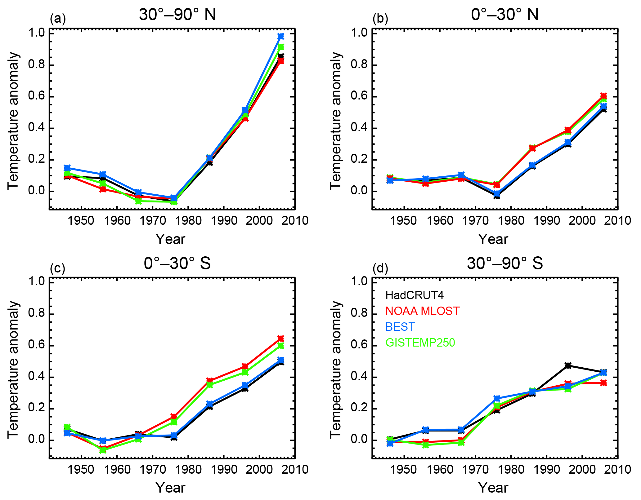
Figure 7Decadal mean temperature anomaly time series derived from the HadCRUT4, NOAA MLOST, BEST, and GISTEMP 250 datasets. Time series are for the four equal-area zonal bands spanning (a) 30–90 ∘N, (b) 0–30 ∘N, (c) 0–30 ∘S, (d) and 30–90 ∘S. Temperatures are plotted as anomalies with respect to the 1906–1995 base period at the midpoint of each decade.
From the time series, we see that while general similarities exist, the model diagnostic depends on which surface observations are used. Across all datasets, we observe the largest signal in the 30–90 ∘N zonal band, consistent with the polar amplification of warming. We also note that the highest agreement across the datasets is observed in this band. We find that there is a separation between the time series in the 0–30 ∘N and 0–30 ∘S zonal bands based on which SST dataset a group used for the temperatures over the ocean. When considering this split, we see similar patterns in the tropical bands between datasets using HadSST (HadCRUT4 and BEST) and datasets using ERSST (MLOST and GISTEMP250). Although not shown, we observe similar patterns in the hemispheric and global mean time series, with a stronger warming signal in the Northern Hemisphere and the time series showing sensitivity to the dataset.
We illustrate how additional data impact the estimate of the linear increase in ocean heat content (Figs. 8 and 9). In both figures, we plot the time series from Levitus et al. (2012) with the pentadal mean plotted at the midpoint of the 5-year period defining the pentad. In Fig. 8, we fix the starting date in 1955 and shift the end date further ahead. In Fig. 9, we fix the length of time over which the linear trend is calculated and shift the entire range forward.
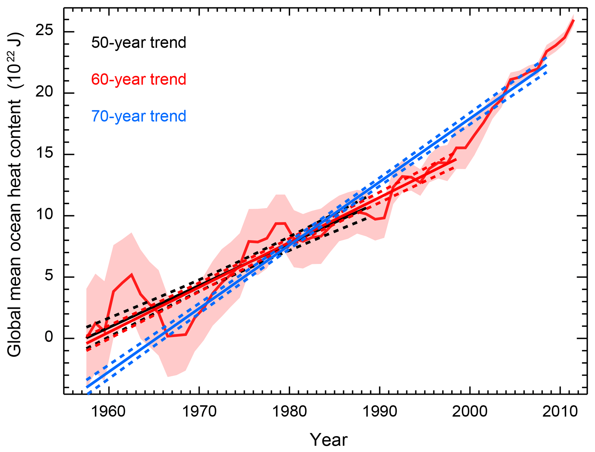
Figure 8Global mean ocean heat content for the 0–2000 m layer. Shading indicates twice the standard error on either side of the estimate. Also shown are the best fit linear trend lines for the trend beginning in 1955 and ending in 1990 (black), 2000 (red), and 2010 (blue). Dashed lines indicate the 95 % confidence interval for the point estimate for a given year based on the best fit line and its uncertainty.
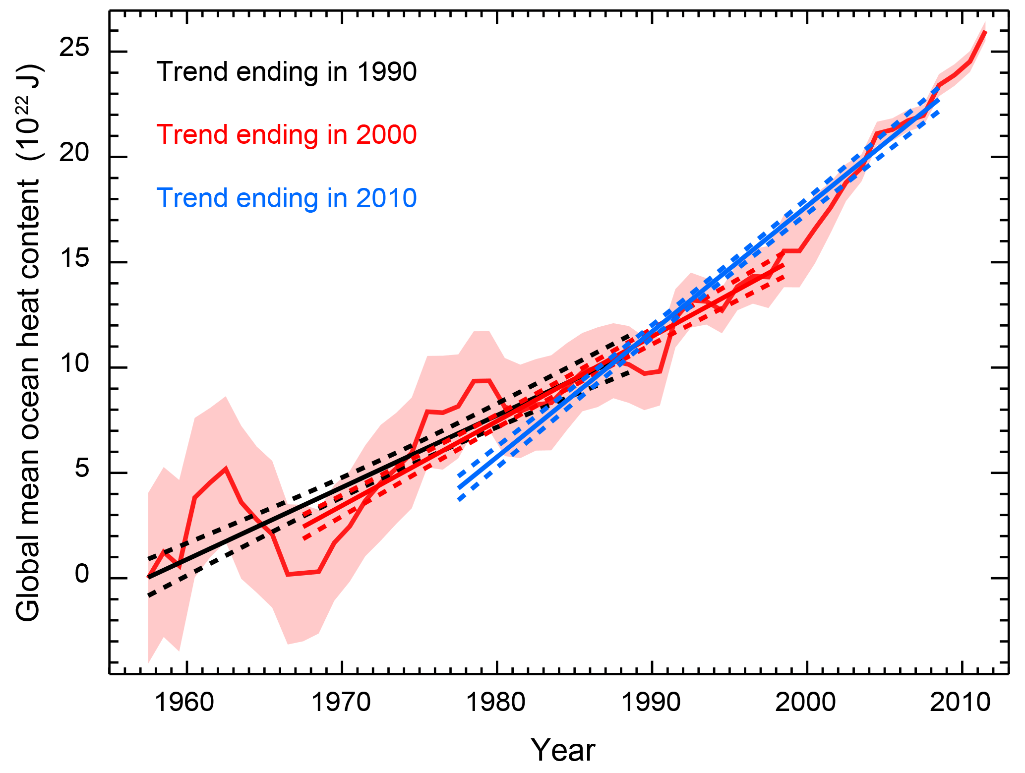
Figure 9As in Fig. 9, except the diagnostic length is held fixed. Linear trend estimates are for the 1955–1990 (black), 1965–2000 (red), and 1975–2010 periods.
The recent acceleration of heat stored in the deep ocean is well documented (Gleckler et al., 2016; Levitus et al., 2012), and as expected, we find that the trend estimate depends on both the end points of the period used for estimation and the length of the period used for estimation. As previously stated, more recent observations have a stronger influence on the trend estimate because the standard error of the observations decreases with time. We calculate higher trend estimates when holding the period length fixed while including more recent data compared to when the period is extended to include more recent data. We estimate a trend of 3.4±0.28 ZJ yr−1 when considering the period from 1955 to 1990. For diagnostics ending in 2000, we estimate a trend of 4.0±0.19 ZJ yr−1 if the starting date is shifted to 1965 and a trend of 3.7±0.15 ZJ yr−1 if the starting date is held at 1955. Trends of 6.0±0.18 and 5.2±0.12 ZJ yr−1 are estimated when using data up to 2010 and holding the diagnostic length fixed and extending the diagnostic length, respectively. By shifting the diagnostic rather than extending it, the accelerated warming signal is stronger because periods of slower warming earlier in the time series are replaced by periods of more rapid warming later in the time series.
For each surface and ocean diagnostic set, we derive joint probability distributions according the experiments discussed in Sect. 2. To account for the different surface temperature datasets, we derive a PDF using each of the four datasets as observations in the surface temperature diagnostic. We combine the four PDFs into a single estimate by taking the average likelihood at each point in the joint PDF. In offline calculations, we confirmed that the marginal PDFs for each parameter using the average joint PDF were nearly identical to the marginal PDFs resulting from the merging method used to submit the distributions from Libardoni and Forest (2013) for inclusion in the Intergovernmental Panel on Climate Change Fifth Assessment Report (Collins et al., 2013). For the IPCC AR5 estimates, we drew a 1000-member Latin hypercube sample from each distribution and calculated marginal distributions for each parameter from the histogram of the drawn values. By including an equal number of samples from each distribution, we assign equal weight to each surface temperature dataset and make no assumption or judgement about whether any dataset is better or worse than the others. Taking the average of the four PDFs is the limit of this method as the number of draws approaches infinity. We justify using the average of the four PDFs by noting that the same general conclusions are drawn from the combined PDF as would be drawn from the PDFs derived from individual datasets.
We first investigate the PDFs by looking for correlations between the model parameters. For each pair of model parameters and for each configuration of the model diagnostics, we calculate the two-dimensional marginal distribution by integrating over the third parameter (Fig. 10). From these distributions, correlations between the pairs of parameters are evident, independent of the diagnostic length and end date. We find ECS and Kv to be positively correlated, ECS and Faer to be negatively correlated, and Kv and Faer to be positively correlated. These correlations make sense when related to the model diagnostics. If we take a fixed surface temperature pattern and conduct a thought experiment for each pair of parameters, the correlations emerge when considering the energy budget at the atmosphere–ocean interface. For a fixed forcing, if climate sensitivity increases, surface temperatures would increase in response to the more efficient heating of the surface. Because these higher temperatures no longer agree with the fixed temperature pattern, a mechanism for removing excess heat from the surface is needed to re-establish balance in the system. In the MESM framework, this mechanism is more efficient mixing of heat into the deep ocean, and thus higher values of Kv. If we fix Kv and again increase ECS so that surface temperatures would increase in response, the mechanism for reducing the energy budget at the surface is the aerosol forcing. To maintain the necessary balance at the surface, Faer needs to be more negative, and is thus negatively correlated with ECS. Lastly, if ECS is fixed, an increase in Kv would remove energy from the surface and tend to cool temperatures. A weaker (less negative) aerosol forcing is needed to maintain the energy balance, indicating that Kv and Faer are positively correlated. Similar arguments follow when considering the ocean heat content diagnostic and the energy budget of the ocean.
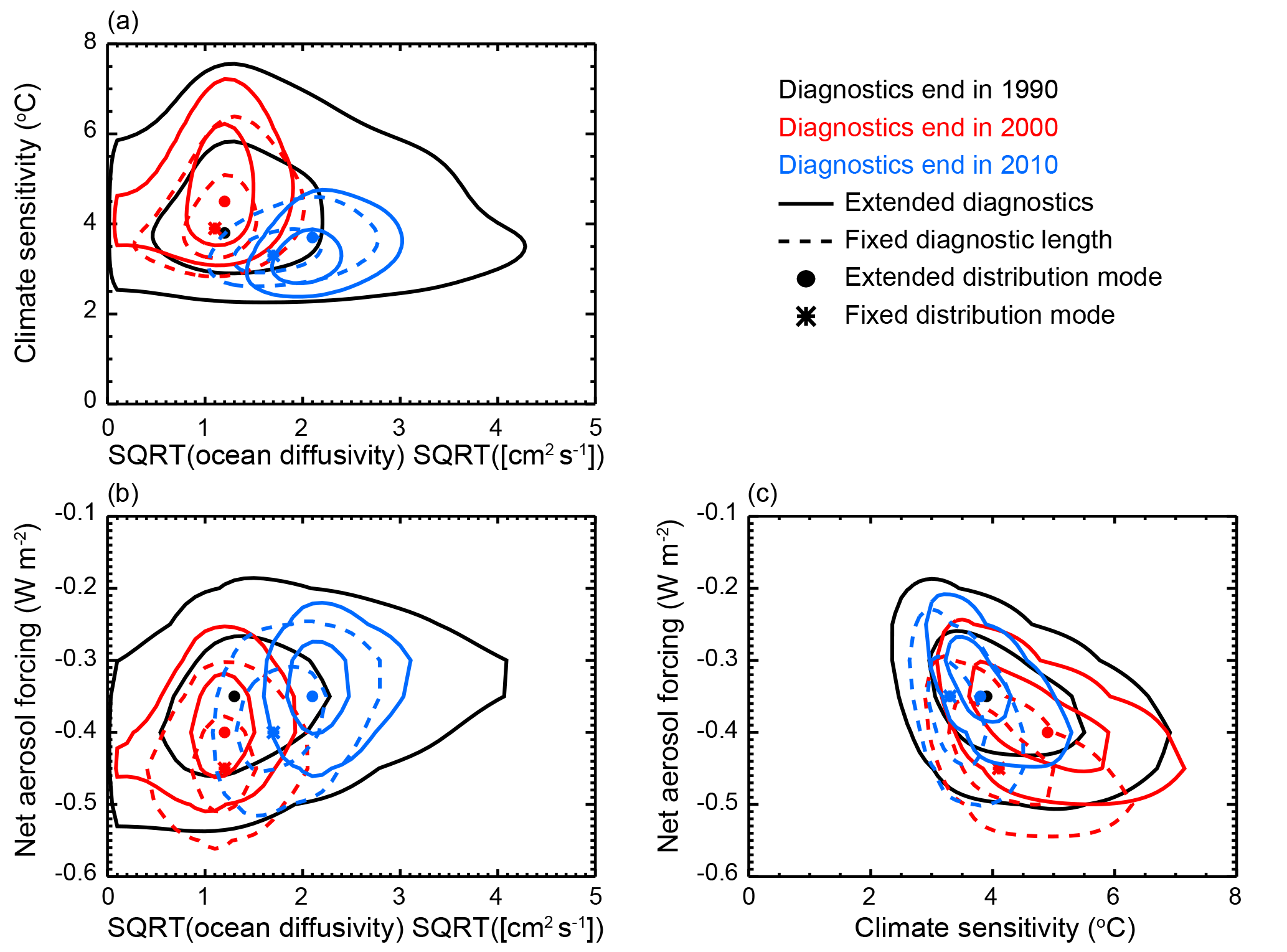
Figure 10Two-dimensional joint probability distribution functions for each pair of parameters: (a) ECS–, (b) Faer–, (c) Faer–CS. Distributions with diagnostics ending in 1990 (black), 2000 (red), and 2010 (blue) are shown. Solid contours indicate an extension of the diagnostic and dashed contours indicate that the lengths of the diagnostics remain fixed when incorporating more recent data. Contours show the 90 % and 50 % credible intervals and symbols indicate the distribution modes.
Second, we show that incorporating more recent data into the temperature diagnostics has a significant impact on the individual parameter estimates by investigating the marginal PDF of each parameter (Fig. 11). Unless otherwise noted, we again approximate the central estimate of the distributions as the median and use the 90 % credible intervals to estimate the uncertainty. Across all three parameters, we generally observe sharper PDFs as more recent data are added. Furthermore, the constraints are stronger when the data are used to extend the diagnostics as opposed to when the diagnostic lengths are fixed. We attribute the general tightening of the distributions with recent data to the strong climate signals that have emerged in the observations. Further, we argue that the uncertainty bounds tend to be tighter when the diagnostic lengths are increased because the model output is being compared against more detailed temperature patterns with additional data points to match. Runs that do not match the added points are rejected for being inconsistent with the observations.
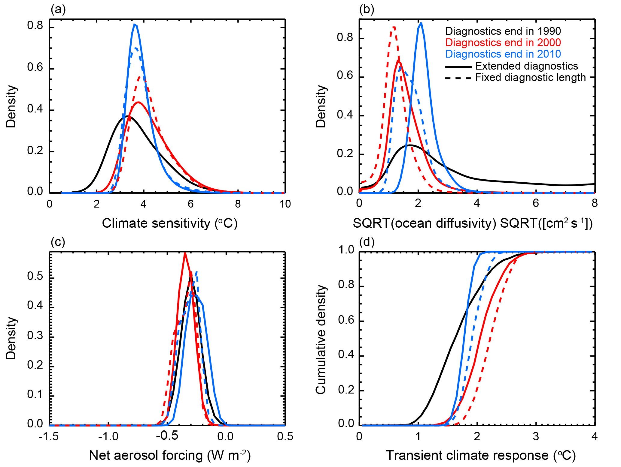
Figure 11Marginal probability distribution functions for (a) ECS, (b) , and (c) Faer, and (d) cumulative distribution function for TCR when changing the end date of model diagnostics. Distributions with diagnostics ending in 1990 (black), 2000 (red), and 2010 (blue) are shown. Solid lines indicate an extension of the diagnostic and dashed lines indicate that the lengths of the diagnostics remain fixed when incorporating more recent data.
For climate sensitivity, we find that extending the data beyond 1990 leads to higher climate sensitivity estimates when compared to the estimate shown in Fig. 6 that incorporates all of the methodological changes. However, we find that the inclusion of more recent data does not always lead to an increase in the estimate of ECS. Our estimate of ECS for diagnostics ending in 2000 is greater than the estimate for the diagnostics ending in 2010, regardless of whether the diagnostic length is extended or fixed. For the case where the diagnostics are extended, we estimate a median climate sensitivity of 4.04 ∘C with data ending in 2000 and 3.73 ∘C with data ending in 2010. When the diagnostic length is fixed, we estimate median climate sensitivities of 4.08 and 3.72 ∘C for diagnostics ending in 2000 and 2010, respectively. We hypothesize that the lowering of the estimate for ECS with diagnostics ending in 2010 can be attributed to the slowing of global mean temperature rise in the 2000s as more heat was stored in the deep ocean. We also note the uncertainty in the estimate of ECS decreases as more recent data are added and the tighter uncertainty bounds come predominantly from a reduction in the upper tail of the distribution. There is also a slight increase in the estimate of the lower bound, however.
Our estimates of Kv show large shifts in response to changes in the diagnostics. When the diagnostics end in 1990, we find a very weak constraint on Kv, with a non-zero tail throughout the domain. As more recent data are included, we see a large reduction in the upper tail of the distributions. We also see shifts towards higher Kv with the inclusion of data from 2001–2010. When including these data, we estimate to increase from 1.45 to 2.08 when the diagnostic lengths increase and from 1.16 to 1.62 when the diagnostic lengths are fixed. Because Kv sets how fast heat is mixed into the deep ocean in the model, we attribute the higher estimates to the recent acceleration of heat storage in the 0–2000 m layer (see Figs. 8 and 9).
We also see shifts in the Faer distribution in response to the changes in model diagnostics. We reiterate that in the MESM, Faer sets the amplitude of the net anthropogenic aerosol forcing and represents the sum of all unmodeled forcings. We observe shifts towards stronger cooling (more negative values of Faer) when diagnostics end in 2000 and shifts back towards weaker values (less negative) when the diagnostics end in 2010. When the diagnostics are extended, estimates shift from −0.28 W m−2 when data up to 1990 are used to −0.32 and −0.23 W m−2 when data up to 2000 and 2010 are used, respectively. Similarly, we observe shifts to −0.32 and −0.28 W m−2 when the diagnostic lengths are held fixed and include data up to 2000 and 2010, respectively. Thus, the observed change from the 2000 to 2010 estimate is larger in the case where the diagnostics are extended rather than of fixed length.
Although not shown, we observe these shifts in the Faer distributions for each of the PDFs derived using the different datasets individually, but note that we see smaller changes with the merged PDF. Also, from the individual PDFs, we see a grouping of the Faer distributions based on the SST dataset used by the research center. We find the HadCRUT4 and MLOST distributions (HadSST) and the BEST and GISTEMP250 distributions (ERSST) to be similar.
We attribute the shift towards stronger cooling for the 1991–2000 decade to the cut-off of the high Kv tail. When Kv decreases, excess heat in the Earth system is stored in the ocean less efficiently. In response to this excess heating, surface and atmospheric temperatures would rise unless an external factor is active and opposes the heating. In the MESM, negative values of Faer reduce the net forcing and contribute to balancing the global energy budget. The spatial pattern of the net aerosol forcing in the MESM leads to the forcing being stronger in the Northern Hemisphere than in the Southern Hemisphere. With this pattern, we observe stronger temperature responses in the Northern Hemisphere when we adjust Faer than we do in the Southern Hemisphere. We attribute the shift back towards weaker aerosol cooling when adding the 2001–2010 trends to the northern hemispheric polar amplification signal noted earlier in this section.
Finally, we derive estimates of transient climate response from the PDFs discussed above (Fig. 11d). From each PDF, we draw a 1000-member Latin hypercube sample and calculate TCR for each of the ECS– pairs using the model response surface derived in Libardoni et al. (2018a). The PDFs of TCR are estimated from the histogram of TCR values with bin size =0.1 ∘C. We show that the TCR estimates reflect changes in the parameter distributions. In particular, TCR and climate sensitivity are positively correlated and TCR and Kv are negatively correlated. Furthermore, the uncertainty in the TCR distribution is correlated with the uncertainty in ECS and Kv. Thus, we find that TCR estimates are greater when more recent data are added due the higher climate sensitivity estimates, but are smaller in 2010 than in 2000 due to the shift towards higher Kv. Furthermore, TCR estimates are higher when the diagnostic lengths are fixed compared to when they are extended.
3.3 Spatial changes to model diagnostics
Until now, we have only considered how the temporal component of the diagnostics impacts the parameter estimates. As a final case study, we reduce the spatial dimension of the surface temperature diagnostic by replacing the four zonal band diagnostic with either global mean surface temperature or hemispheric mean temperatures using the 1941–2010 diagnostic period (Fig. 12). Similar to the PDFs shown when changing the temporal structure of the diagnostic, we present the distributions calculated from the average of the four individual PDFs derived using the different surface temperature datasets.
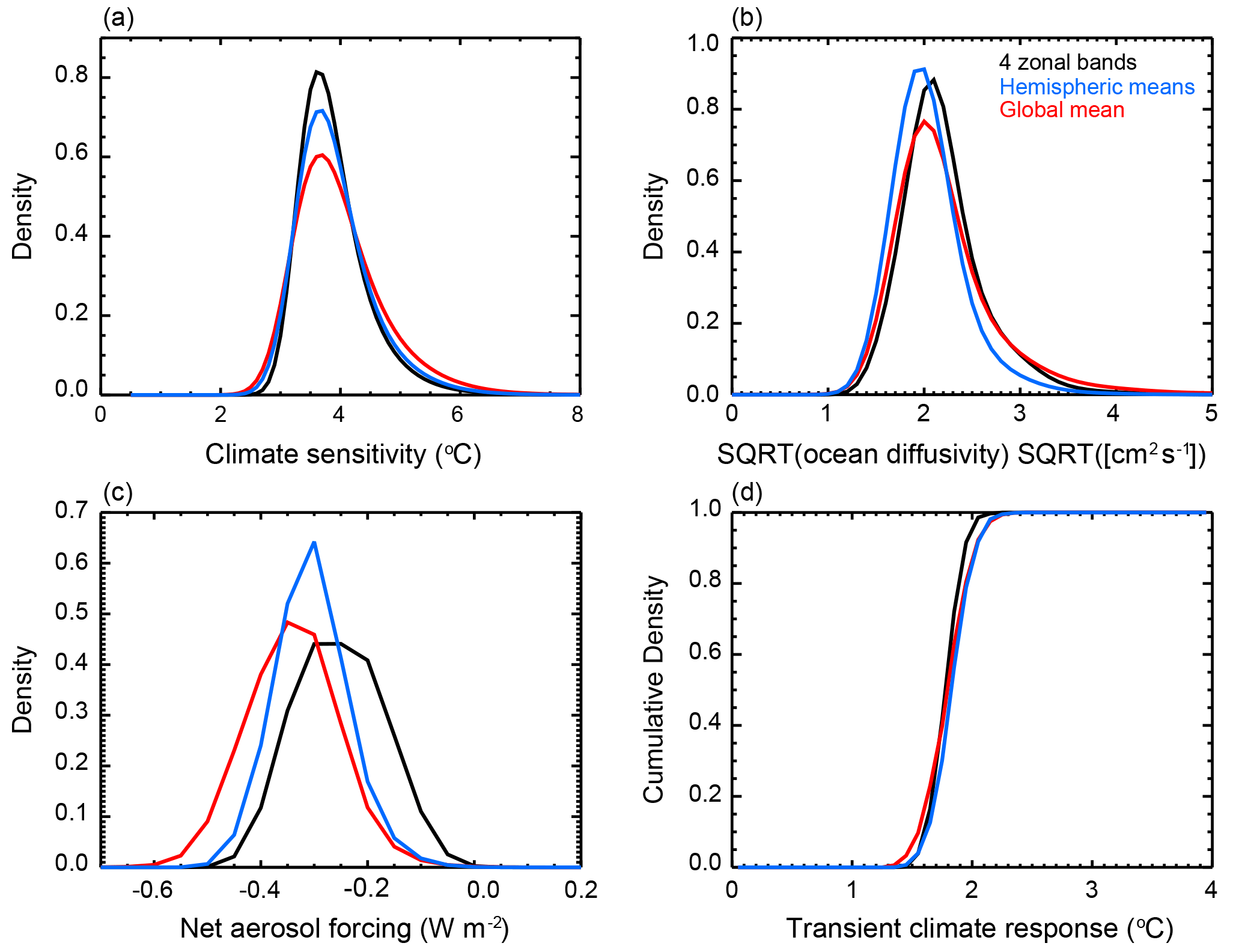
Figure 12Marginal probability distribution functions for (a) ECS, (b) , and (c) Faer and (d) cumulative distribution function for TCR derived from different spatial diagnostics. Diagnostics end in 2010 and data are added by extending the diagnostics.
We find little sensitivity in the central estimates of the ECS and Kv distributions to the spatial structure of the surface diagnostic using data up to 2010. For , the median estimate for when global mean temperatures, hemispheric means, and four zonal bands are used are 3.81, 3.75, and 3.72 ∘C, respectively. Similarly, median estimates for are 2.06, 1.94, and 2.08 when global mean, hemispheric mean, and four zonal mean temperatures are used. However, we observe a tightening of the distributions as the spatial resolution of the surface diagnostic increases. The narrowest distributions are derived using the four zonal band diagnostic and the widest distributions are derived using global mean temperatures. We note that the TCR distributions follow the shifts in ECS and Kv. Thus, the central estimates do not change significantly, but the width of the distribution shrinks as spatial information is added to the surface diagnostic.
Unlike with the ECS and Kv distributions, we observe a sensitivity to the surface diagnostic structure in the Faer distributions. In particular, we observe that the estimate derived using global mean temperature leads to the strongest (most negative) aerosol forcing and the estimate derived using the four zonal bands leads to the weakest aerosol forcing. When considering only global mean temperature, we remove the polar amplification signal from the temperature diagnostic. Removing this signal means that we ignore the spatial dependence of the aerosol distribution and only consider the net effect on the global energy budget. However, as we include variations of temperature with latitude, the spatial pattern of the aerosol forcing pattern matters. As a result, the median estimate of shifts from −0.31 to −0.28 to −0.23 W m−2 when global mean, hemispheric mean, and four zonal bands are used. Thus, while the spatial structure has only a small influence on ECS and Kv, it has a strong influence on Faer.
We implement a number of methodological changes to improve probability estimates of climate system properties. Changes include switching to an interpolation based on radial basis functions, estimating natural variability from a common model across diagnostics, using new observational datasets, and incorporating recent temperature changes in model diagnostics. We show that the parameter estimates follow signals in the data and depend on the model diagnostics. Furthermore, we show that the technical changes, namely the interpolation method and the natural variability estimate, do not considerably change the central estimate of the parameters, but do impact the uncertainty estimates of the distributions.
We have shown that the RBF interpolation method is successful in smoothing the distributions while not changing the central estimate. The success of the RBF method is an encouraging sign for future research. Due to the two-dimensional interpolation method previously used, our work until now has been restricted to running ensembles on a uniform grid of points in the parameter space. The RBF method is three-dimensional and can be applied to any collection of node points. We can thus run the full model at any set of non-gridded nodes and interpolate the goodness-of-fit statistics to estimate the values at intermediate points. Other studies (Olson et al., 2012; Sansó and Forest, 2009) have built statistical emulators to approximate model output at non-node parameter settings for each point in the diagnostic time series and then calculate the likelihood function by comparing the emulator output to observations. We argue that by interpolating the metrics, rather than model output at individual points in the time series, we approximate the impact of all feedbacks on the diagnostic together, rather than individually at different spatial and temporal scales.
Our results suggest that the spatial structure of model diagnostics plays a key role in the estimation of parameters with spatial variation. When adding spatial structure to the diagnostics, we observed little change in parameters representing global mean quantities (ECS and Kv), but the distributions of Faer differed depending on whether global mean temperature, hemispheric mean temperatures, or temperatures in four equal-area zonal bands were used. When global diagnostics are used, we ignore the spatial variation of forcing patterns and fail to account for regional influences on climate change. Our estimates provide an assessment of the importance of these spatial patterns when estimating probability distributions for model parameters.
Overall, our work highlights that recent temperature trends have a strong influence on the parameter distributions. In particular, we observe a shift in the distributions towards higher climate sensitivity due to the addition of recent surface temperature warming trends relative to 1990, but with a reduction in the estimate when using data up to 2010 as opposed to 2000. We also observe that the distributions of Kv shift towards higher values. The uncertainty in our estimates decreases as more recent data are used in the temperature diagnostics. Our estimates of transient climate response reflect the changes in ECS and Kv and are correlated with ECS and anticorrelated with Kv. By incorporating more recent data, which are of higher quality, and using improved methodology, we are more confident in our estimates of the model parameters and transient climate response.
The source code of MESM will become publicly available for non-commercial research and educational purposes as soon as a software license that is being prepared by the MIT Technology Licensing Office is complete. For further information contact mesm-request@mit.edu. All data required to reproduce the figures in the main text and scripts to replicate the figures are available. Model output is available upon request.
As discussed in Sect. 2, when estimating r2 at intermediate points, the weight assigned node point values in the radial basis function interpolation is a function of the distance between the two points. We have normalized the parameter space for each parameter by the range sampled in the 1800-member ensemble of MESM runs so that each dimension is isometric in the distance calculation. In this normalized space, the grid spacing for each model parameter is
The weight of any node point in the calculation of r2 at an interpolated point is given in Eq. (5) and is a function of the distance between the points and the scaling parameter ϵ. When first developing the algorithm, we hypothesized that having each node point influence the r2 value at an interpolated point within three grid points in model parameter space would achieve the fit and smoothness we sought from the interpolation. Because the grid spacing in normalized space is not equal for the three parameters, we chose an average of the three individual spacings and used 0.1 as the approximate distance of one grid space. Setting d=0.3 and ϕ=0.01 to account for the distance between three nodes and the weight approaching zero at that distance, respectively, we solve for ϵ=7.2.
To test other ϵ values, we scaled the original choice by factors of 0.5, 1.5, and 2. For ϵ=3.6, we calculate an e-folding distance of 0.27. This implies a large sphere of influence, as the weight decays to 0.37 at a distance of approximately three grid points away in normalized parameter space. Thus, rather than decay to zero as for the original estimate, there is still significant influence from the node point at d=0.3. This leads to the over-smoothing of the r2 pattern observed in Fig. 3. In similar calculations, we determine e-folding distances in normalized parameter space of 0.09 and 0.07 for ϵ=10.8 and ϵ=14.4, respectively. For ϵ=10.8, this implies an e-folding distance of approximately one grid space in the and Faer dimensions, while for ϵ=14.4, the weight has decayed to 0.13 at a distance of one grid space in those dimensions. Using larger values of ϵ leads to further decay of the weighting function one normalized grid point away from the nodes. We chose ϵs of 17.2 and 21.2 to demonstrate this feature.
AL and AS carried out the MESM simulations. AS wrote the codes for extracting model output. AL performed the analysis and prepared the original manuscript. AL and CF developed the model ensemble and experimental design. AL, CF, AS, and EM all contributed to interpreting the analysis and synthesizing the findings.
The authors declare that they have no conflict of interest.
This work was supported by the U.S. Department of Energy (DOE), Office of
Science, under award DE-FG02-94ER61937, and other government, industry, and
foundation sponsors of the MIT Joint Program on the Science and Policy of
Global Change. For a complete list of sponsors and U.S. government funding
sources, see https://globalchange.mit.edu/sponsors/current
(last access: 25 November 2018). The authors would like to
thank the National Climatic Data Center, the Hadley Centre for Climate
Prediction and Research, and the NASA Goddard Institute for Space Studies for
producing publicly available surface data products and the NOAA National
Centers for Environmental Information for providing publicly available ocean
heat content data. We would also like to thank the University of Maryland for
access to the Evergreen high-performance computing cluster for model
simulations. Alex Libardoni also recognizes the valuable discussions and
suggestions made by Ken Davis, Klaus Keller, and Ray Najjar in the development of
this work.
Edited by: Francis
Zwiers
Reviewed by: two anonymous referees
Aldrin, M., Holden, M., Guttorp, P., Skeie, R. B., Myhre, G., and Bernstein, T. K.: Bayesian estimation of climate sensitivity based on a simple climate model fitted to observations of hemispheric temperatures and global ocean heat content, Environmetrics, 23, 253–271, 2012. a, b
Andrews, D. G. and Allen, M. R.: Diagnosis of climate models in terms of transient climate response and feedback response time, Atmos. Sci. Lett., 9, 7–12, 2008. a
Andronova, N. G. and Schlesinger, M. E.: Objective estimation of the probability density function for climate sensitivity, J. Geophys. Res., 106, 22605–22612, 2001. a
Bayes, T.: An essay towards solving a problem in the doctrine of chances, Phil. Trans. Roy. Soc., 53, 370–418, 1763. a
Bindoff, N. L., Stott, P. A., AchutaRao, K. M., Allen, M. R., Gillett, N., Gutzler, D., Hansingo, K., Hegerl, G., Gu, Y., Jain, S., Mokhov, I. I., Overland, J., Perlwitz, J., Sebbari, R., and Zhang, X.: Detection and attribution of climate change: From global to regional, in: Climate Change 2013: The Physical Science Basis. Contribution of Working Group I to the Fifth Assessment Report of the Intergovernmental Panel on Climate Change, edited by: Stocker, T., Qin, D., Plattner, G.-K., Tignor, M., Allen, S., Boschung, J., Nauels, A., Xia, Y., Bex, V., and Midgley, P., 867–952, Cambridge University Press, Cambridge, UK and New York, NY, USA, 2013. a
Brohan, P., Kennedy, J. J., Harris, I., Tett, S. F. B., and Jones, P. D.: Unceratainty estimates in regional and global observed temperature changes: A new data set from 1850, J. Geophys. Res., 111, D12106, https://doi.org/10.1029/2005JD006548, 2006. a
Collins, M. M. R. K., Arblaster, J., Dufresne, J.-L., Fichefet, T., Friedlingstein, P., Gao, X., Gutowski, W., Johns, T., Krinner, G., Shongwe, M., Tebaldi, C., Weaver, A., and Wehner, M.: Long-term climate change: Projections, commitments and irreversibility, in: Climate Change 2013: The Physical Science Basis. Contribution of Working Group I to the Fifth Assessment Report of the Intergovernmental Panel on Climate Change, edited by: Stocker, T., Qin, D., Plattner, G.-K., Tignor, M., Allen, S., Boschung, J., Nauels, A., Xia, Y., Bex, V., and Midgley, P., 1029–1136, Cambridge University Press, Cambridge, UK and New York, NY, USA, 2013. a
Cowtan, K. and Way, R. G.: Coverage bias in the HadCRUT4 temperature series and its impact on recent temperature trends, Q. J. Roy. Meterol. Soc., 140, 1935–1944, 2014. a
Forest, C. E., Allen, M. R., Sokolov, A. P., and Stone, P. H.: Constraining climate model properties using optimal fingerprint detection methods., Clim. Dynam., 18, 277–295, 2001. a
Forest, C. E., Stone, P. H., Sokolov, A. P., Allen, M. R., and Webster, M. D.: Quantifying uncertainties in climate system properties with the use of recent climate observations, Science, 295, 113–117, 2002. a
Forest, C. E., Stone, P. H., and Sokolov, A. P.: Estimated PDFs of climate system properties including natural and anthropogenic forcings, Geophys. Res. Let., 33, L01705, https://doi.org/10.1029/2005GL023977, 2006. a, b, c, d
Forest, C. E., Stone, P. H., and Sokolov, A. P.: Constraining climate model parameters from observed 20th century changes, Tellus, 60A, 911–920, 2008. a, b, c
Gent, P. R., Danabasoglu, G., Donner, L. J., Holland, M. M., Hunke, E. C., Jayne, S. R., Lawrence, D. M., Neale, R. B., Rasch, P. J., Vertenstein, M., Worley, P. H., Yang, Z.-L., and Zhang, M.: The Community Climate System Model Version 4, J. Climate, 24, 4973–4991, https://doi.org/10.1175/2011JCLI4083.1, 2011. a
Gleckler, P. J., Durack, P. J., Stouffer, R. J., Johnson, G. C., and Forest, C. E.: Industrial-era global ocean heat uptake doubles in recent decades, Nat. Clim. Change, 6, 394–398, 2016. a, b
Hansen, J., Ruedy, R., Sato, M., and Lo, K.: Global surface temperature change, Rev. Geophys., 48, RG4004, https://doi.org/10.1029/2010RG000345, 2010. a
Huang, B., Banzon, V. F., Freeman, E., Lawrimore, J., Liu, W., Peterson, T. C., Thorne, T. M. S. P. W., Woodruff, S. D., and Zhang, H.-M.: Extended Reconstructed Sea Surface Temperature Version 4 (ERSST.v4). Part I: Upgrades and intercomparisons, J. Climate, 28, 911–930, 2015. a
Huber, M. and Knutti, R.: Natural variability, radiative forcing and climate response in the recent hiatus reconciled, Nat. Geosci., 7, 651–656, 2014. a, b
Johansson, D. J. A., O'Neill, B. C., Tebaldi, C., and Haggstrom, O.: Equilibrium climate sensitivity in light of observations over the warming hiatus, Nat. Clim. Change, 5, 449–453, 2015. a, b
Karl, T., Arguez, A., Huang, B., Lawrimore, J., McMahon, J., Menne, M., Peterson, T., Vose, R., and Zhang, H.-M.: Possible artifacts of data biases in the recent global surface warming hiatus, Science, 348, 1469–1472, 2015. a
Kennedy, J. J., Rayner, N. A., Smith, R. O., Parker, D. E., and Saunby, M.: Reassessing biases and other uncertainties in sea surface temperature observations measured in situ since 1850: 1. Measurement and sampling uncertainties, J. Geophys. Res.-Atmos., 116, D14103, https://doi.org/10.1029/2010JD015218, 2011a. a
Kennedy, J. J., Rayner, N. A., Smith, R. O., Parker, D. E., and Saunby, M.: Reassessing biases and other uncertainties in sea surface temperature observations measured in situ since 1850: 2. Biases and homogenization, J. Geophys. Res.-Atmos., 116, D14104, https://doi.org/10.1029/2010JD015220, 2011b. a
Knutti, R. and Tomassini, L.: Constraints on the transient climate response from observed global temperature and ocean heat uptake, Geophys. Res. Lett., 35, L09701, https://doi.org/10.1029/2007GL032904, 2008. a
Knutti, R., Stocker, T. F., Joos, F., and Plattner, G.-K.: Constraints on radiative forcing and future climate change from observations and climate model ensembles, Nature, 416, 719–723, 2002. a
Knutti, R., Stocker, T. F., Joos, F., and Plattner, G.: Probabilistic climate change projections using neural networks, Clim. Dynam., 21, 257–272, 2003. a
Levitus, S., Antonov, J., and Boyer, T.: Warming of the world ocean, 1955–2003, Geophys. Res. Lett., 32, L02604, https://doi.org/10.1029/2004GL021592, 2005. a, b
Levitus, S., Antonov, J. I., Boyer, T. P., Baranova, O. K., Garcia, H. E., Locarnini, R. A., Mishonov, A. V., Reagan, J. R., Seidov, D., Yarosh, E. S., and Zweng, M. M.: World ocean heat content and thermosteric sea level change (0–2000 m), 1955–2010, Geophys. Res. Lett., 39, L10603, https://doi.org/10.1029/2012GL051106, 2012. a, b, c, d, e, f
Lewis, N.: An objective Bayesian improved approach for applying optimal fingerprint techniques to climate sensitivity, J. Climate, 26, 7414–7429, https://doi.org/10.1175/JCLI-D-12-00473.1, 2013. a
Libardoni, A. G. and Forest, C. E.: Sensitivity of distributions of climate system properties to the surface temperature dataset, Geophys. Res. Lett., 38, L22705, https://doi.org/10.1029/2011GL049431, 2011. a, b, c, d
Libardoni, A. G. and Forest, C. E.: Correction to ”Sensitivity of distributions of climate system properties to the surface temperature data set”, Geophys. Res. Lett., 40, 2309–2311, https://doi.org/10.1002/grl.50480, 2013. a, b, c, d
Libardoni, A. G., Forest, C. E., Sokolov, A. P., and Monier, E.: Baseline evaluation of the impact of updates to the MIT Earth System Model on its model parameter estimates, Geosci. Model Dev., 11, 3313–3325, https://doi.org/10.5194/gmd-11-3313-2018, 2018a. a, b, c, d, e, f
Libardoni, A., Forest, C., Sokolov, A., and Monier, E.: Underestimating internal variability leads to narrow estimates of climate system properties, in preparation, 2018b. a
McKay, M. D., Beckman, R. J., and Conover, W. J.: A comparison of three methods for selecting values of input variables in the analysis of output from a computer code, Technometrics, 21, 239–245, 1979. a
Meehl, G. A., Arblaster, J. M., Fasullo, J. T., Hu, A., and Trenberth, K. E.: Model-based evidence of deep-ocean heat uptake during surface-temperature hiatus periods, Nat. Clim. Change, 1, 360–364, 2011. a, b
Meinshausen, M., Meinshausen, N., Hare, W., Raper, S., Frieler, K., Knutti, R., Frame, D., and Allen, M.: Greenhouse-gas emission targets for limiting global warming to 2 degrees C, Nature, 458, 1158–1162, 2009. a
Morice, C. P., Kennedy, J. J., Rayner, N. A., and Jones, P. D.: Quantifying uncertainties in global and regional temperature change using an ensemble of observational estimates: The HadCRUT4 data set, J. Geohpys. Res., 117, D08101, https://doi.org/10.1029/2011JD017187, 2012. a
Olson, R., Sriver, R., Goes, M., Urban, N. M., Matthews, H. D., Haran, M., and Keller, K.: A climate sensitivity estimate using Bayesian fusion of instrumental observations and an Earth System model, J. Geophys. Res., 117, D04103, https://doi.org/10.1029/2011JD016620, 2012. a, b, c, d
Powell, M. J. D.: Restart procedures for the conjugate gradient method, Math. Prog., 12, 241–254, 1977. a
Rohde, R., Muller, R. A., Jacobsen, R., Muller, E., Perlmutter, S., Rosenfeld, A., Wurtele, J., Groom, D., and Wickham, C.: A new estimate of the average Earth surface and land temperature spanning 1753 to 2011, Geoinfor. Geostat: An Overview, 1:1, https://doi.org/10.4172/2327-4581.1000101, 2013. a
Sansó, B. and Forest, C.: Statistical calibration of climate system properties, Appl. Statist., 58, 485–503, 2009. a
Schmidt, G., Shindell, D. T., and Tsigaridis, K.: Reconciling warming trends, Nat. Geosci., 7, 158–160, 2014. a, b
Skeie, R. B., Berntsen, T., Aldrin, M., Holden, M., and Myhre, G.: A lower and more constrained estimate of climate sensitivity using updated observations and detailed radiative forcing time series, Earth Syst. Dynam., 5, 139–175, https://doi.org/10.5194/esd-5-139-2014, 2014. a
Sokolov, A., Schlosser, C., Dutkiewicz, S., Paltsev, S., Kicklighter, D., Jacoby, H., Prinn, R., Forest, C., Reilly, J., Wang, C., Felzer, B., Sarofim, M., Scott, J., Stone, P., Melillo, J., and Cohen, J.: The MIT Integrated Global System Model (IGSM) Version 2: Model description and baseline evaluation, Joint Program Report Series, Report 124, 40 pp., 2005. a
Sokolov, A., Kicklighter, D., Schlosser, A., Wang, C., Monier, E., Brown-Steiner, B., Prinn, R., Forest, C., Gao, X., Libardoni, A., and Eastham, S.: Description and evaluation of the MIT Earth System Model (MESM), J. Adv. Model Earth Syst., 10, 1759–1789, 2018. a
Sokolov, A. P., Forest, C. E., and Stone, P. H.: Comparing oceanic heat uptake in AOGCM transient climate change experiments, J. Climate, 16, 1573–1582, 2003. a
Tomassini, L., Reichert, P., Knutti, R., Stocker, T. F., and Borsuk, M. E.: Robust Bayesian uncertainty analysis of climate system properties using Markov Chain Monte Carlo estimates, J. Climate, 20, 1239–1254, 2007. a, b
Trenberth, K. E. and Fasullo, J. T.: An apparent hiatus in global warming?, Earth's Future, 1, 19–32, 2013. a
Urban, N. M. and Keller, K.: Complementary observational constraints on climate sensitivity, Geophys. Res. Lett., 36, L04708, https://doi.org/10.1029/2008GL036457, 2009. a, b
Urban, N. M., Holden, P. B., Edwards, N. R., Sriver, R. L., and Keller, K.: Historical and future learning about climate sensitivity, Geophys. Res. Lett., 41, 2543–2552, 2014. a, b
Vose, R. S., Arndt, D., Banzon, V. F., Easterling, D. R., Gleason, B., Huang, B., Kearns, E., Lawrimore, J. H., Menne, M. J., Peterson, T. C., Reynolds, R. W., Smith, T. M., Williams Jr., C. N., and Wuertz, D. B.: NOAA's merged land–ocean surface temperature analysis, B. Am. Meteorol. Soc., 93, 1677–1685, 2012. a
Webster, M. and Sokolov, A.: A methodology for quantifying uncertainty in climate projections, Clim. Change, 46, 417–446, 2000. a