Comparing forecast systems with multiple correlation decomposition based on partial correlation

The multiple correlation and/or regression information that two competing forecast systems have on the same observations is decomposed into four components, adapting the method of multivariate information decomposition of Williams and Beer (2010), Wibral et al. (2015), and Lizier et al. (2018). Their concept is to divide source information about a target into total, (target) redundant or shared, and unique information from each source. It is applied here to the comparison of forecast systems using classic regression. Additionally, non-target redundant or shared information is newly defined that resumes the redundant information of the forecasts which is not observed. This provides views that go beyond classic correlation differences. These five terms share the same units and can be directly compared to put prediction results into perspective. The redundance terms in particular provide a new view. All components are given as maps of explained variance on the observations and for the non-target redundance on the models, respectively. Exerting this concept to lagged damped persistence is shown to be related to directed information entropy. To emphasize the benefit of the toolkit on all timescales, two analysis examples are provided. Firstly, two forecast systems of the German decadal prediction system of “Mittelfristige Klimaprognose”, namely the pre-operational version and a special version using ensemble Kalman filter for the ocean initialization, are compared. The analyses reveal the clear added value of the latter and provide an as yet unseen map of their non-target redundance. Secondly, 4 d lead forecasts from the European Centre for Medium-Range Weather Forecasts (ECMWF) are compared to a simple autoregressive and/or damped persistence model. The analysis of the information partition on this timescale shows that interannual changes in damped persistence, seen as target redundance changes between forecasts and damped persistence models, are balanced by associated changes in the added value of the dynamic forecasts in the extratropics but not in the tropics.

1 Introduction

A classic method for determining the potential skill of a forecast system versus observations is the use of the Pearson correlation coefficient, which is directly related to information entropy. The comparison of competing forecast systems is another basic issue in the evaluation of forecasting systems, for example, for quality assurance purposes. For the Pearson correlation metric, this problem is often addressed using correlation differences. However, a central problem in the comparison of different forecasting systems is the strong collinearity of the two forecasting systems because, by construction, both systems aim at a reproduction of the same observations. DelSole and Tippett (2014) and Siegert et al. (2017) introduced and tested different methods to account for collinearity. Hering and Genton (2011) demonstrated a test procedure that is robust to this problem, and Gilleland et al. (2018) showed that the block bootstrap is also reasonably accurate. While not specifically discussing correlation, correlation can be utilized as what they term the loss function.

Another way to overcome this problem is the use of partial correlations, which at the same time offers new views for forecast evaluation. The use of partial correlations has the advantage of well-known methods for inference; for example, hypothesis testing. Partial correlations can be tested like conventional correlations after reducing the degrees of freedom accordingly (Anderson, 1984).

The method of partial correlations can be related to the partial information decomposition (PID) which has been proposed by Williams and Beer (2010). This paper attracted a significant amount of attention, which led to a special issue on “Information Decomposition of Target Effects from Multi-Source Interactions” in the journal Entropy (Lizier et al., 2018). The terminology of the PID, i.e. total, redundant or shared, and unique information is taken from Williams and Beer (2010) and Lizier et al. (2018). There is not yet a global consensus on a general redundancy measure (Lizier et al., 2018).

Here a partial correlation decomposition (PCD) is applied under the assumption of continuous Gaussian distributed variables for which the mutual information is directly related to multiple correlation. Multiple correlation of one target variable and multiple predictands is the classic Pearson correlation between a variable and its regression on the predictands (Anderson, 1984). Classic sample estimates of Pearson correlation and regression coefficients (Anderson, 1984) are used to determine total, redundant, and unique information estimates from data. We have added to the PID a redundance term that shows shared information between the models and/or predictands that is not found in the observations and/or targets. We will concentrate on the case of comparing two systems which makes the approach most clear.

The redundant or shared information between the forecasting systems on the observations is named target redundance here. The unique information is the added value that one forecast provides when given the other. The newly defined component is non-target redundance, which is that part of the shared variance between the models not verified by observations. The first three components can be depicted as four maps of explained variances on the observations, whereby the added values are separately determined for each of the models. The non-target redundance is based on the same partial correlation for both models but is mapped using the individual unexplained variance of the respective model, given the observations. Details of the derivation and definitions are outlined in Sects. 2 and 3.

We will present results of the PCD for two examples covering different timescales. The first is an application to decadal climate forecasts using two versions of the ensemble prediction system developed within the German decadal climate prediction project of MiKliP (Marotzke et al., 2016; Polkova et al., 2019; Brune and Baehr, 2020). The second example concentrates on medium-range forecasts from ECMWF, taken from the THORPEX Interactive Grand Global Ensemble (TIGGE) database (Swinbank et al., 2016). The data are described in Sect. 4, and the results are given Sects. 5 and 6.

2 Multiple and partial correlation coefficients

The comparison of the pros and cons of two different forecast systems can be done within the framework of correlation. The starting point here is the multiple correlation coefficient (Anderson, 1984, p. 40, Eq. 15), which reflects the correlation between the observations and their multivariate regression on both forecasts. The multiple correlation is a measure of the total information that can be derived from both forecasts on the observations. The associated partial correlations (Anderson, 1984) describe the correlations of each of the model time series with the residual of the observational time series that is not explained by a linear regression of the opposing model. The partial correlations are transformed to the unique information that is the added value of each of the forecasts. It is that part of the observational variance uniquely explained by one of the models. The difference between the total and the unique information from each of the models is the target redundant information. It is that part of the variance information which both forecast models share in the observations.

By indexing the observations with 1 and the two forecast systems with 2 and 3, the multiple linear regression of the observations in the two forecasts is given by the following:

$$\begin{array}{}\text{(1)}& \stackrel{\mathrm{̃}}{X_{\mathrm{1}}}={\mathit{\mu }}_{\mathrm{1}}+\mathit{\beta }(X_{\mathrm{2}},X_{\mathrm{3}}{)}^t,\end{array}$$

where β is the matrix of regression coefficients (Anderson, 1984). The squared multiple correlation coefficient $R_{\mathrm{1}\left(\mathrm{23}\right)}^{\mathrm{2}}$ is defined as the Pearson correlation between X₁ and ${\stackrel{\mathrm{̃}}{X}}_{\mathrm{1}}$.

$$\begin{array}{}\text{(2)}& \begin{array}{rl}{R}_{\mathrm{1}\left(\mathrm{23}\right)}^{\mathrm{2}}& ={\mathit{\rho }}_{\mathrm{1}\stackrel{\mathrm{̃}}{\mathrm{1}}}^{\mathrm{2}}\\ & ={\mathit{\rho }}_{\mathrm{12}}^{\mathrm{2}}+{\mathit{\rho }}_{\mathrm{13}\cdot \mathrm{2}}^{\mathrm{2}}(\mathrm{1}-{\mathit{\rho }}_{\mathrm{12}}^{\mathrm{2}})\\ & ={\displaystyle \frac{{\mathit{\rho }}_{\mathrm{12}}^{\mathrm{2}}+{\mathit{\rho }}_{\mathrm{13}}^{\mathrm{2}}-\mathrm{2}{\mathit{\rho }}_{\mathrm{12}}{\mathit{\rho }}_{\mathrm{13}}{\mathit{\rho }}_{\mathrm{23}}}{\mathrm{1}-{\mathit{\rho }}_{\mathrm{23}}^{\mathrm{2}}}}.\end{array}\end{array}$$

The second equation for $R_{\mathrm{1}\left(\mathrm{23}\right)}^{\mathrm{2}}$ in Eq. (2) shows how the multiple correlation can be built up hierarchically when including additional predictors. Both equations are given in Anderson (1984) and Yule (1907). A third equation is obtained by replacing the partial correlation with their representations as correlations (Eq. 4).

In the case of Gaussian random observations and simulations, it can be shown that the multiple correlation is directly linked to information entropy (I). Information entropy is the relative entropy between a joint and its marginal distributions. The expressions for the relative entropy of Gaussian distributions are given in Kleeman (2002). The relation between the ratio of the determinant of the joint covariance matrix and the product of the determinants of the marginal distributions is given in Anderson (1984, p. 40, Eq. 16).

$$\begin{array}{}\text{(3)}& I_{\mathrm{1}\left(\mathrm{23}\right)}={\displaystyle \frac{\mathrm{1}}{\mathrm{2}}}\ln \left({\displaystyle \frac{\mathrm{1}}{\mathrm{1}-R_{\mathrm{1}\left(\mathrm{23}\right)}^{\mathrm{2}}}}\right).\end{array}$$

This relation justifies the application of the partial information decomposition to multiple correlations.

The partial (conditional) correlation ρ_12⋅3 (Anderson, 1984, p. 41, Eq. 20) between variable 1 and 2, given 3, is as follows:

$$\begin{array}{}\text{(4)}& {\mathit{\rho }}_{\mathrm{12}\cdot \mathrm{3}}={\displaystyle \frac{{\mathit{\rho }}_{\mathrm{12}}-{\mathit{\rho }}_{\mathrm{13}}{\mathit{\rho }}_{\mathrm{23}}}{\sqrt{\mathrm{1}-{\mathit{\rho }}_{\mathrm{13}}^{\mathrm{2}}}\sqrt{\mathrm{1}-{\mathit{\rho }}_{\mathrm{23}}^{\mathrm{2}}}}}.\end{array}$$

Note that there are three different partial correlations made available by the three possible permutations of the indices. The direct comparison of the partial correlations ρ_12⋅3 and the corresponding ρ_13⋅2 can be misleading, even if both are equally large. This is because the calculation of the partial correlation of forecast system 2, given forecast system 3, is based on the residuum of the observations after linear regression using forecast system 3. In the case of a small residuum, even a high partial ${\mathit{\rho }}_{\mathrm{12}\cdot \mathrm{3}}^{\mathrm{2}}$ represents only a small fraction of variance on the observations. A more informative measure of the unique information is the additionally explained fraction of the total observational variance. We define this fraction as the added value ${\mathit{\rho }}_{+\mathrm{12}\cdot \mathrm{3}}^{\mathrm{2}}$. It describes the increase in total correlation and/or explained variance due to one model, given the other, as can be seen in Eq. (2).

$$\begin{array}{}\text{(5)}& {\mathit{\rho }}_{+\mathrm{12}\cdot \mathrm{3}}^{\mathrm{2}}={\mathit{\rho }}_{\mathrm{12}\cdot \mathrm{3}}^{\mathrm{2}}\left(\mathrm{1}-{\mathit{\rho }}_{\mathrm{13}}^{\mathrm{2}}\right)={\displaystyle \frac{{\left({\mathit{\rho }}_{\mathrm{12}}-{\mathit{\rho }}_{\mathrm{13}}{\mathit{\rho }}_{\mathrm{23}}\right)}^{\mathrm{2}}}{\mathrm{1}-{\mathit{\rho }}_{\mathrm{23}}^{\mathrm{2}}}}.\end{array}$$

Mapping this quantity is more intuitive than partial correlation because it describes the additionally explained variance on the observations, while the squared partial correlation gives the explained variance relative to the as yet unexplained part left by the competing model, which varies locally.

From Eqs. (5) and (4) it follows that the difference in the added values of the models equals the difference of their squared correlations with the observations. Thus, the target redundant information drops out from squared correlation differences. The conditional variance or mean square error between the observations and their linear regression on one of the forecasts is MSE${}_{\mathrm{1}i}={\mathit{\sigma }}_{\mathrm{1}}^{\mathrm{2}}\left(\mathrm{1}-{\mathit{\rho }}_{\mathrm{1}i}^{\mathrm{2}}\right)$ (Anderson, 1984, p. 37, Eq. 9). Thus the difference between the two regression errors is also proportional to the difference in the added values.

$$\begin{array}{}\text{(6)}& {\mathit{\rho }}_{+\mathrm{12}\cdot \mathrm{3}}^{\mathrm{2}}-{\mathit{\rho }}_{+\mathrm{13}\cdot \mathrm{2}}^{\mathrm{2}}={\mathit{\rho }}_{\mathrm{12}}^{\mathrm{2}}-{\mathit{\rho }}_{\mathrm{13}}^{\mathrm{2}}={\displaystyle \frac{{\mathrm{MSE}}_{\mathrm{13}}-{\mathrm{MSE}}_{\mathrm{12}}}{{\mathit{\sigma }}_{\mathrm{1}}^{\mathrm{2}}}}.\end{array}$$

This shows that two competing forecasting systems may be compared on the basis of the univariate correlation coefficients, provided that the differences of the squared correlations are taken. Depending on the sign of the difference, the relative advantage of either forecasting system can be specified. However, the individual advantages are only summarized by the added values from Eq. (5). Besides the multiple correlation and added value of the respective forecasts, the target redundance R_rr1(23) can be derived. It is information provided equally by both systems. According to Williams and Beer (2010), Wibral et al. (2015), and Lizier et al. (2018), the redundant information of a three component system with two predictors and one predictand is the difference between the total information and the unique information of each predictor. When applied to the multiple correlation, this is the difference between the multiple correlation and the added values of each of the two forecasts.

$$\begin{array}{}\text{(7)}& \begin{array}{rl}{R}_{rr\mathrm{1}\left(\mathrm{23}\right)}^{\mathrm{2}}& =R_{\mathrm{1}\left(\mathrm{23}\right)}^{\mathrm{2}}-({\mathit{\rho }}_{+\mathrm{12}\cdot \mathrm{3}}^{\mathrm{2}}+{\mathit{\rho }}_{+\mathrm{13}\cdot \mathrm{2}}^{\mathrm{2}})\\ & ={\displaystyle \frac{\mathrm{2}{\mathit{\rho }}_{\mathrm{12}}{\mathit{\rho }}_{\mathrm{13}}{\mathit{\rho }}_{\mathrm{23}}-({\mathit{\rho }}_{\mathrm{12}}^{\mathrm{2}}+{\mathit{\rho }}_{\mathrm{13}}^{\mathrm{2}}){\mathit{\rho }}_{\mathrm{23}}^{\mathrm{2}}}{\mathrm{1}-{\mathit{\rho }}_{\mathrm{23}}^{\mathrm{2}}}}.\end{array}\end{array}$$

The target redundance is a base level for the ranking of the two competitive forecasting systems. To our knowledge, the expression has not been derived before and, at least, not been used in the context of prediction ranking.

Besides the target redundance term, there is a portion of the variance of the competing forecasting systems which is potentially not represented in the observations. This portion we define as non-target redundance. It goes beyond the PID of Williams and Beer (2010), Wibral et al. (2015), and Lizier et al. (2018). It is derived from the third available partial correlation ρ_23⋅1 in terms of the variances one obtains, namely ${\mathit{\rho }}_{+\mathrm{23}\cdot \mathrm{1}}^{\mathrm{2}}$ and ${\mathit{\rho }}_{+\mathrm{32}\cdot \mathrm{1}}^{\mathrm{2}}$, respectively. These values describe those variance parts of either forecasting system which are common to the two systems but not represented in the observations. It provides a detailed look at systematic model errors and can be interesting to model developers. It is the partial correlation squared ${\mathit{\rho }}_{\mathrm{23}\cdot \mathrm{1}}^{\mathrm{2}}$ of the models, given the observation multiplied by the respective remaining variance when predicting the forecasts, using the observations as predictors.

$$\begin{array}{}\text{(8)}& \begin{array}{rl}{\mathit{\rho }}_{\mathrm{23}\cdot \mathrm{1}}^{\mathrm{2}}& ={\displaystyle \frac{({\mathit{\rho }}_{\mathrm{23}}-{\mathit{\rho }}_{\mathrm{12}}{\mathit{\rho }}_{\mathrm{13}}{)}^{\mathrm{2}}}{(\mathrm{1}-{\mathit{\rho }}_{\mathrm{12}}^{\mathrm{2}})(\mathrm{1}-{\mathit{\rho }}_{\mathrm{13}}^{\mathrm{2}})}},\\ {\mathit{\rho }}_{+\mathrm{23}\cdot \mathrm{1}}^{\mathrm{2}}& ={\mathit{\rho }}_{\mathrm{23}\cdot \mathrm{1}}^{\mathrm{2}}(\mathrm{1}-{\mathit{\rho }}_{\mathrm{21}}^{\mathrm{2}})={\displaystyle \frac{({\mathit{\rho }}_{\mathrm{23}}-{\mathit{\rho }}_{\mathrm{12}}{\mathit{\rho }}_{\mathrm{13}}{)}^{\mathrm{2}}}{\mathrm{1}-{\mathit{\rho }}_{\mathrm{13}}^{\mathrm{2}}}}.\end{array}\end{array}$$

The variables of the PCD form a uniform tool that can be used in various combinations. They are partly more or less established and partly new (Table 1). Besides the new views provided by the redundance terms, the use of multiple correlation and added values, instead of regression coefficients and correlation differences, allows one to directly compare these quantities.

Table 1 PCD terms.

3 Partial correlation and directed information

The concept of partial correlation is also useful for distinguishing actual model forecasts from simplified forecasts such as damped persistence and/or autoregressive models of the observations. Runge et al. (2014) used this methodology in a comparable manner to evaluate information fluxes in a cross-correlation analysis. They tried to distinguish the information flux across meteorological fields from time-lagged autocorrelations. In the context of information theory, the term directed information comes into play. This is the information that moves from one variable to another one within one time step. It is defined as the average information that goes from variable X to Y over N time steps (Massey, 1990; Harremoës, 2006; Quinn et al., 2011).

$$\begin{array}{}\text{(9)}& \stackrel{\mathrm{̃}}{I}\left(X^N\to Y^N\right)={\displaystyle \frac{\mathrm{1}}{N}}\sum _{n=\mathrm{1}}^{N}I\left(Y_n;X_{\mathrm{1}}^{n-\mathrm{1}}|Y_{\mathrm{1}}^{n-\mathrm{1}}\right).\end{array}$$

In the case of the current topic of prediction evaluation, the mean information gained from a model forecast that goes beyond damped persistence is determined in this manner. It is the conditional information of the forecasts, given the damped persistence model. A continuous form of Eq. (9) can be written out under the assumption that the mutual information rate exists (Quinn et al., 2011). It can be determined from the difference between the information entropies of the joint probability distribution of the observations (again labelled 1) and their damped persistence series (labelled 3) versus the forecast (labelled 2) and the information entropy between the forecast and the observed persistence model.

$$\begin{array}{}\text{(10)}& \begin{array}{rl}& {\stackrel{\mathrm{̃}}{I}}_{\mathrm{2}\to \mathrm{1}}=I_{\mathrm{21}\cdot \mathrm{3}}=I_{\mathrm{12}\cdot \mathrm{3}}\\ & =I_{\left(\mathrm{13}\right)\mathrm{2}}-I_{\mathrm{23}}\\ & ={\displaystyle \frac{\mathrm{1}}{\mathrm{2}}}\ln \left({\displaystyle \frac{\mathrm{1}}{\mathrm{1}-R_{\mathrm{2}\left(\mathrm{13}\right)}^{\mathrm{2}}}}\right)-{\displaystyle \frac{\mathrm{1}}{\mathrm{2}}}\ln \left({\displaystyle \frac{\mathrm{1}}{\mathrm{1}-{\mathit{\rho }}_{\mathrm{32}}^{\mathrm{2}}}}\right)\\ & =-{\displaystyle \frac{\mathrm{1}}{\mathrm{2}}}\ln {\displaystyle \frac{\mathrm{1}-R_{\mathrm{2}\left(\mathrm{13}\right)}^{\mathrm{2}}}{\mathrm{1}-{\mathit{\rho }}_{\mathrm{23}}^{\mathrm{2}}}}.\end{array}\end{array}$$

The first equality is the continuous form for Eq. (9); the second and third are derived from Eqs. (3a) and (4) of Harremoës (2006). The last two relations hold for Gaussian processes. They can be deduced following the relative entropy derivation for Gaussian processes (Kleeman, 2002). Equation (2) relates the conditional and multiple correlation and can be used to write the argument of the logarithm in the bottom line of Eq. (10) in terms of conditional correlation.

$$\begin{array}{}\text{(11)}& {\mathit{\rho }}_{\mathrm{21}\cdot \mathrm{3}}^{\mathrm{2}}=\mathrm{1}-{\displaystyle \frac{\mathrm{1}-R_{\mathrm{2}\left(\mathrm{13}\right)}^{\mathrm{2}}}{\mathrm{1}-{\mathit{\rho }}_{\mathrm{23}}^{\mathrm{2}}}}={\mathit{\rho }}_{\mathrm{12}\cdot \mathrm{3}}^{\mathrm{2}}.\end{array}$$

Thus, the partial correlation can be directly related to directed information entropy. $R_{\mathrm{2}\left(\mathrm{13}\right)}^{\mathrm{2}}$ can be determined from Eq. (2). It is the correlation between the forecasts and its linear regression on the observations and the damped persistence model. Thus, partial correlation is a direct tool for determining the information flux from an external variable, given the observed damped persistence information.

4 Examples

In the following, the decomposition of multiple correlation analysis using partial correlations is applied to the verification of a multi-annual ensemble mean 2 m temperature time series (1961–2013) from two decadal ensemble prediction systems of the German MiKlip decadal forecast project (Marotzke et al., 2016) and to synoptic daily 2 m temperature forecasts from ECMWF for three winters. In a forecast system, one does not expect negative correlations or distinguish meaningfully between negative and less negative correlations. Therefore, negative correlations have been trimmed and set to zero.

4.1 Data

First, annual mean 2 m temperatures for the period 1962–2013 averaged over lead years 2 to 5 are examined. They are taken from initialized retrospective decadal climate hindcasts as part of the MiKlip decadal climate prediction system (Polkova et al., 2019; Kadow et al., 2016). Two sets of model simulations are compared. For both sets, the external forcing is prescribed according to the Coupled Model Intercomparison Project Phase 5 (CMIP5; Taylor et al., 2012) until 2005 and to the RCP4.5 pathway from 2006 onwards (Giorgetta et al., 2013). Both are based on the MPI-ESM (version 1.2) in the low-resolution configuration of MPI-ESM-LR (Giorgetta et al., 2013). The two versions are a pre-operational version (PREOP; Polkova et al., 2019) and an experimental one, which utilizes a localized ensemble Kalman filter (EnKF) initialization (Polkova et al., 2019; Brune et al., 2015) for the ocean model component. In the atmospheric component, both the PREOP and the EnKF system use full-field nudging of vorticity, divergence, temperature, and sea level pressure for the ERA40 and/or ERA-Interim reanalyses (Uppala et al., 2005; Dee et al., 2011). In the oceanic component, PREOP uses anomaly nudging of temperature and salinity for ORAS4 reanalysis (Balmaseda et al., 2013), whereas the EnKF directly assimilates the observed temperature and salinity profiles from the EN4 database (Good et al., 2013).

All decadal forecasts start on 1 November each year and consider the first 2 months (November and December) as the spin-up phase. Thus, lead year 2 actually starts after 14 months of integration time. The correlation analysis is done on the ensemble mean of 10 available ensemble members in each forecast system, beginning in January in the year following the initialization. The forecasts are evaluated using the HadCRUT4 (Morice et al., 2012) data set as observations. The model data are interpolated to the observational grid with a grid size of $\mathrm{5}{}^{\circ }\times \mathrm{5}{}^{\circ }$ and blended with the observational mask of available data.

The second example compares daily mean ECMWF forecasts at lead +4 d with a damped persistence or autoregressive model for the three winter seasons during December–January–February (DJF) from 2014–2015 to 2016–2017. The forecasts are available on a global grid with a $\mathrm{0.5}{}^{\circ }\times \mathrm{0.5}{}^{\circ }$ grid distance. The daily mean is defined as the average of the forecasts at 00:00 and 12:00 Coordinated Universal Time (UTC) (Owens and Hewson, 2018). Here only the deterministic forecasts are taken from The Observing system Research and Predictability EXPERIMENT (THORPEX; Swinbank et al., 2016). These forecasts are evaluated relative to the respective analyses on the verifying days.

4.2 Sensitivity of decadal climate predictions to initialization procedures

Within the MiKlip project for decadal hindcasts, the EnKF model version, based on the ensemble Kalman initialization technique for ocean temperature initialization, has been tested and compared to nudging methods to initialize the model ensemble for ocean and atmosphere reanalyses (Polkova et al., 2019; Brune and Baehr, 2020). Here the comparison of EnKF and PREOP for 2 m temperature, based on the partial correlation approach for means of lead years 2 to 5, are presented. As in Polkova et al. (2019), the HadCRUT4 data set serves as the observational basis.

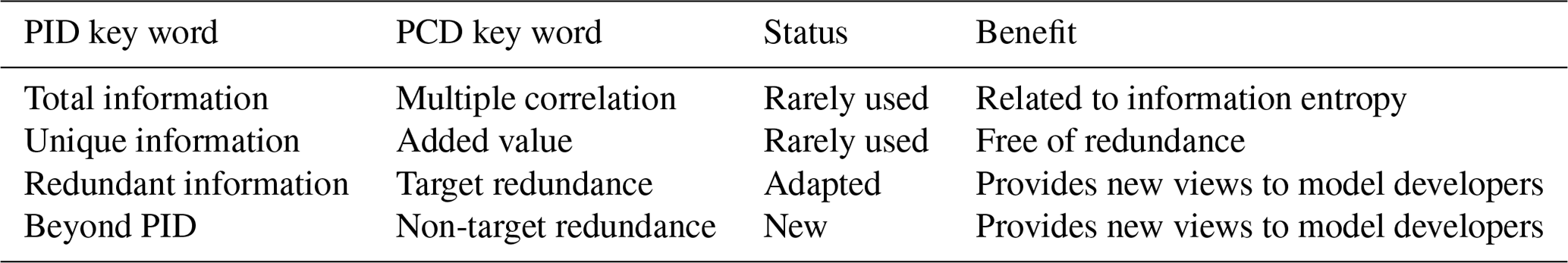
Figure 1 shows the multiple correlation of the observations with both forecast systems and the target redundance. As outlined above, this is the explained variance on the observations by the shared part of both forecasting systems. Even the shared variance between both systems is relatively large on this timescale over many regions. This is due to the prescribed external forcings, which include the anthropogenic forcing. The focus here is, however, on the differences in model performance. Figure 2 depicts the unique information that is the added values of each system with respect to the corresponding other forecast system. The larger values of multiple correlation can be found over regions of Africa, enhancing the target redundance where it is already relatively large, but also over the eastern Pacific Ocean, where the target redundance values are close to zero.

Figure 2 depicts the unique information that is the added value of each system with respect to the corresponding other forecast system. An added value is mainly seen for the EnKF version of the MiKlip prediction system. Over some key regions above the North Atlantic, Africa, north and tropical eastern Pacific Ocean, more than 20 % of variance can be explained additionally using the EnKF initialization instead of the nudging method in PREOP. One advantage of this representation is that one can compare the added values in terms of additionally explained variance on the observations as a map. The better performance of the EnKF above the Pacific Ocean results from an improved modelling of the sea surface temperatures (SSTs) due to the assimilation of observed temperature and salinity profiles. This, in turn, improved the surface temperature forecasts, which are closely related to the SSTs in this region, even on a 2–5 year timescale. The 4-year averaging was chosen to filter out the El Niño effects in order to look for potential predictability on this timescale that goes beyond El Niño predictability.

The test of the null hypothesis of vanishing added values has been determined using the Student t test of the respective partial correlations evaluated at the 5 % significance value. The necessary number of sampling steps is taken as the number of time steps n divided by four due to the averaging over lead years 2 to 5. In the current example, the added value of the PREOP system with respect to the EnKF is very small, so the multiple correlation is nearly equal to the classic squared Pearson correlation of the EnKF system, and the target redundance is close to the squared Pearson correlation of the PREOP system with observations.

The non-target redundance of EnKF and PREOP is shown in Fig. 3. These coherent variability patterns are nearly identical, indicating that, in the regions of non-target redundance, the residual variance not common with the observations is similar in both forecasting systems. Especially over the subtropical Pacific Ocean, broad bands of non-target redundance, reaching 40 % to 60 % of the total model variance, can be found. Similar levels are found over the southern tropical Atlantic. Actually, over most parts of the world, coherent non-target redundance can be found. Small non-target redundance values are found over the northern Pacific and North Atlantic oceans, where the EnKF model version has regions of pronounced added value, explaining the observations compared to the PREOP. It is tempting to conclude that these matching structures of the non-target redundance indicate a common and erroneous behaviour of the underlying coupled atmosphere–ocean–land surface model beyond the usually presented systematic error.

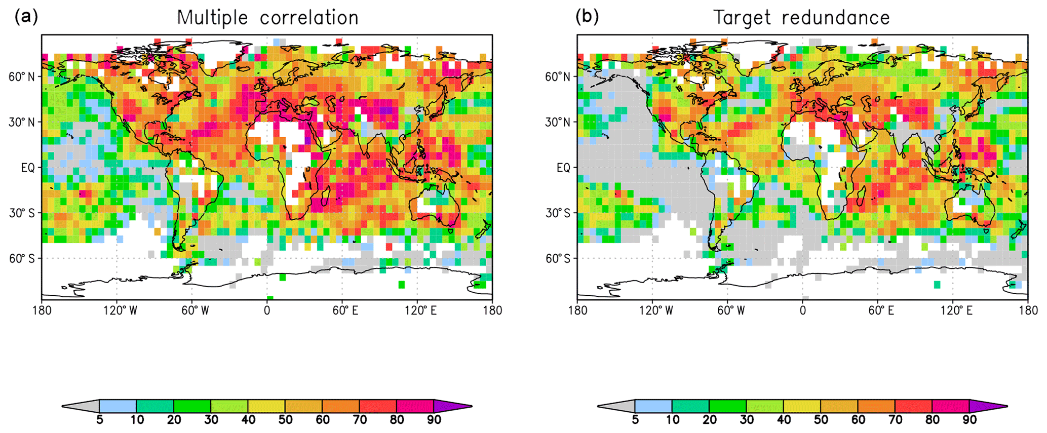
Figure 1 Squared multiple correlation coefficients (a) and target redundances (b) between 2 m temperature from HadCRUT4 observations and two MiKlip ensemble forecasts, namely the ensemble Kalman filter (EnKF) and pre-operational version (PREOP), for lead years 2 to 5. Units are a fraction of the explained variance in the observations in percentages. Assuming a Student t distribution of the R² estimates, and about 13 degrees of freedom, the confidence intervals R² (in percentages) are $\mathrm{14}<\mathrm{60}<\mathrm{85}$, $\mathrm{26}<\mathrm{70}<\mathrm{90}$, and $\mathrm{45}<\mathrm{80}<\mathrm{94}$.

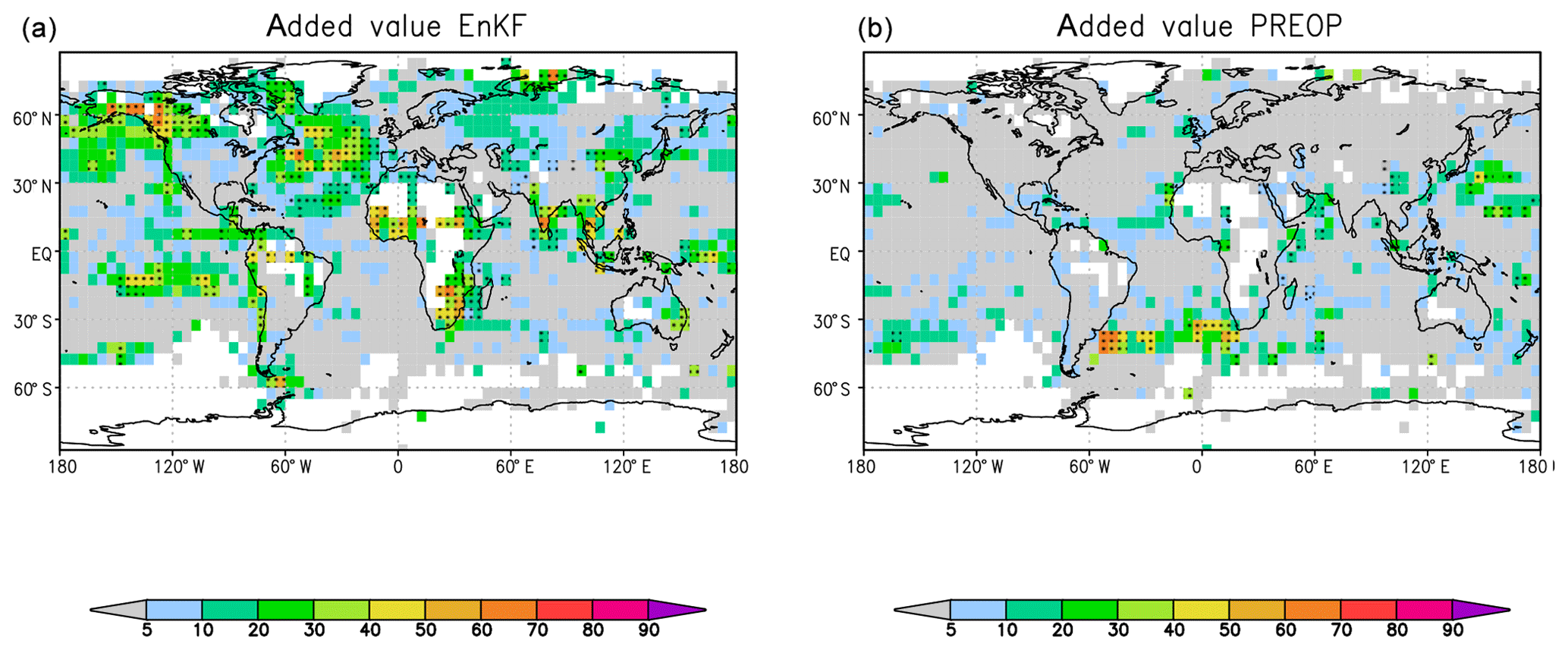
Figure 2 As in Fig. 1 but for added values from partial correlations between HadCRUT4 and EnKF, given PREOP, (a) and between HadCRUT4 and PREOP, given EnKF (b). Black dots indicate where the partial correlations are above the 5 % significance level.

Figure 3 As in Fig. 1 but for non-target redundances in EnKF (a) and in PREOP (b). Units are a fraction of the explained variance in the respective model in percentages.

4.3 ECMWF lead day 4 forecasts compared to analysis and damped persistence

Lead day 4 dynamic model forecasts and lag day −4 damped persistence and/or autoregressive model forecasts are concurrently compared to analyses for each of the three winters from 2014–2015 to 2016–2017. The individual single seasons are analysed to see how far the dynamic model can compensate for interannual changes in persistence. Furthermore, the annual cycle is already part of the damped persistence model, so the added value of the dynamic model with respect to the latter goes beyond annual cycle simulation. This comparative analysis of dynamic and damped persistent models is related to the directed information theory discussed in Sect. 3.

The multiple correlations for the winter of 2016–2017 are given in Fig. 4a. Over large parts of the extratropics, the explained variance by the forecasts lies above 60 % or even higher. However, in the tropics there is a zone along the Equator where the multiple correlations are only about half of those at midlatitudes. In fact, this multiple correlation is, in this case, equal to the squared correlation between analysis and forecast because the damped persistence has no added value with respect to the dynamic model. The target redundance (Fig. 5) shows the information that can be similarly drawn from the lead day 4 forecasts and from a damped −4 d persistence forecast. Thus, this information is already present in the local time series and is not added by the dynamic model forecast. Areas of large redundance between the dynamic and the damped persistence model are present, especially in the subtropics and tropics.

Generally similar results are found for the other two winters. We want, however, to analyse the interannual differences. Figure 4b shows the difference in the multiple correlations between the winters of 2016–2017 and 2014–2015. There are larger multiple correlations in the winter of 2016–2017 in the eastern Pacific Ocean, extending from the South American continent and into the Caribbean Sea, in the southeastern Pacific Ocean, near the southeastern coast of Africa, from the southern part of Madagascar into the Indian Ocean, and on the eastern coast of Australia. Negative regions are found in the southern Atlantic extending to central Africa and the northern Indonesian regions. Similar but partly enhanced features can be found in the differences in the target redundance, which is here bounded by the damped persistence model in Fig. 5, especially near the Bering Strait, above the North Atlantic extending to northwestern Africa, and in the southeastern Pacific Ocean and near the southeastern coast of Africa. In these regions, the reduced added values (blue regions in Fig. 6b) of the lead 4 d forecast, compared to the damped persistence of the winter in 2016–2017 relative to the winter in 2014–2015, partly compensates for the increased target redundance in the later winter. The situation is different in the region that extends from the Horn of Africa into the interior of the continent where the multiple correlations are higher for the winter of 2014–2015 compared to 2016–2017 (Fig. 4). The target redundance difference Fig. 5 is also negative, indicating stronger damped persistence during the winter of 2014–2015. But the differences are larger than the multiple correlation differences because the added value of the 4 d forecasts (Fig. 6) partly compensates for the smaller redundances and/or persistences in the winter of 2016–2017. The same is true for parts of the negative bands in the South Atlantic and for the region between Greenland and North America. In this region, large changes in persistence are fully compensated by the added value of the lead day 4 dynamic forecasts; accordingly, the multiple correlation differences are negligible. In summary, changes in forecast quality between the different years can be assessed in comparison to changes in the persistence of the system. Higher quality predictions only due to increased system persistence might be of less value than an increase in added value. Furthermore, even if the quality does not change over the years, the compensation between changes in target redundance and added values may indicate the additional power of the prediction system.

Next, we look for the general tendency for compensation between changes in the lag day −4 damped persistence forecasts and the associated changes in the added value of the dynamic 4 d forecasts. The results show that there is a general tendency for compensation to occur in the extratropics. Figure 7a shows a scatter diagram of the changes in target redundance between the winters of 2016–2017 and 2014–2015 in Fig. 5 and the changes in added values in Fig. 6 for the region 120^∘ W–120^∘ E and 30–70^∘ N. The Pacific region has been excluded because it is partly dominated by the El Niño phenomenon. The scatter diagram shows a strong negative relationship between these quantities and, thus, an indication for compensation between reduced persistence and increased added value of the dynamic forecasts for that region. On the other hand, in Fig. 7b a close relationship is visible for the tropical band between 10^∘ S and 10^∘ N, i.e. the target redundance changes in Fig. 5 and the changes in multiple correlation in Fig. 4. Apparently, the persistence changes are not balanced by increased added values of the dynamic forecasts in the tropics.

Figure 4 Squared multiple correlations between ECMWF reanalyses and ECMWF lead day 4 dynamic forecasts and damped lag day −4 persistence forecasts for the winter (December–January–February – DJF) of 2016–2017 (a). Differences between the multiple correlation coefficients for the winters of 2016–2017 and 2014–2015 (b). Assuming a Student t distribution of the R² estimates, and about 18 degrees of freedom, the confidence intervals R² (in percentages) are $\mathrm{22}<\mathrm{60}<\mathrm{83}$, $\mathrm{35}<\mathrm{70}<\mathrm{86}$ and $\mathrm{55}<\mathrm{80}<\mathrm{92}$.

Figure 5 As in Fig. 4 but for target redundances of ECMWF lead day 4 dynamic forecasts and damped lag day −4 persistence forecasts for the winter of 2016–2017 (a). Differences in the target redundances between the winters of 2016–2017 and 2014–2015 (b).

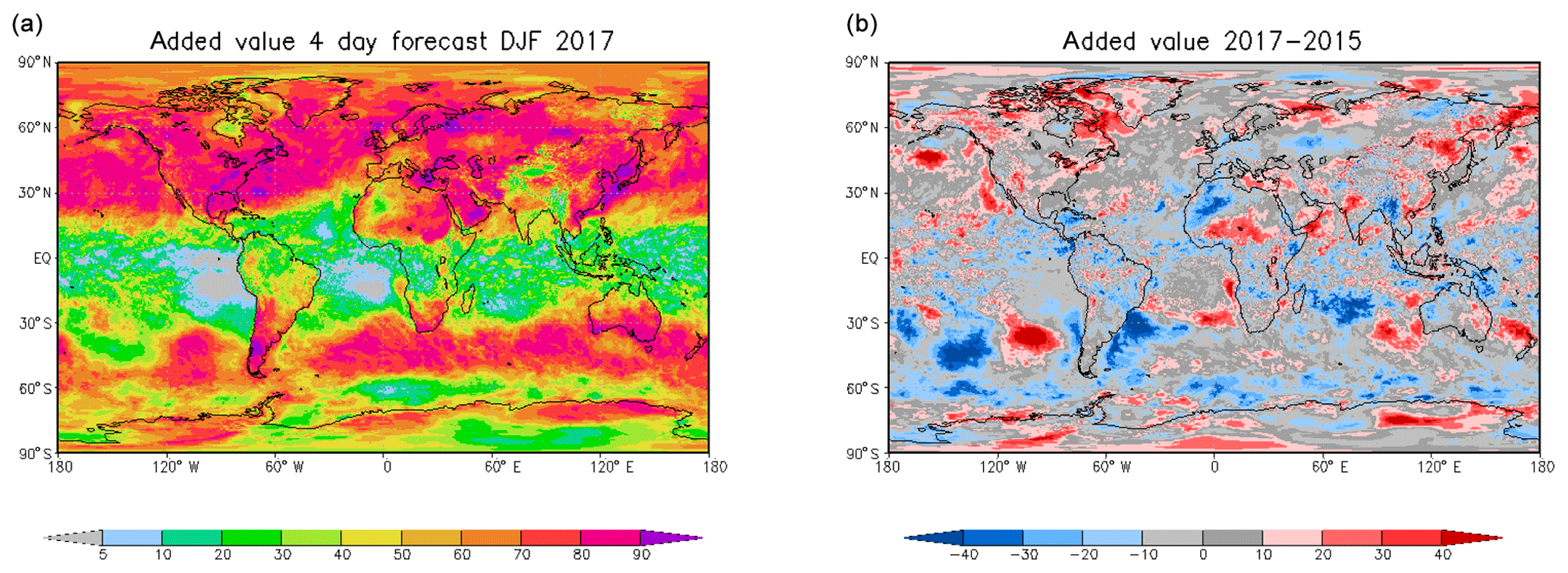
Figure 6 As in Fig. 4 but for added values of ECMWF lead day 4 dynamic forecasts of 2 m temperature with respect to damped lag day −4 persistence forecasts for the winter of 2016–2017 (a). Differences in the added values between the winters of 2016–2017 and 2014–2015 (b).

Figure 7 Scatter diagrams in which the target redundance differences between the winters of 2016–2017 and 2014–2015 of 4 d dynamic and damped lag day −4 persistence forecasts are assigned to the x axis, and the differences in added values of 4 d dynamic forecasts for 120^∘ E, 120^∘ W, and 30–70^∘ N are assigned to the y axis (a). The differences in the multiple correlations of 4 d dynamic and damped lag day −4 persistence forecasts hemispherically for 10^∘ S to 10^∘ N are assigned to the y axis in (b). The Pacific Ocean extratropics are excluded in (a) because they behave more like the tropics, probably because they are influenced by El Niño–Southern Oscillation (ENSO). In the extratropics, increases and/or decreases in damped persistence, here seen as target redundance changes, are balanced by opposite decreases and/or increases in added values. In the tropics, however, increases and/or decreases in damped persistence lead to increased and/or lower forecast quality or multiple correlations.

5 Conclusions

In this paper, we proposed an as yet unexplored method for evaluating and comparing two opposing forecasting systems with the respective observations on the basis of correlation and/or regression partial decomposition. Apart from the classic views provided by regressions, correlations, and differences, two new variates are presented. One is the shared variance between both models and the observations, and the other is the shared variance between the models that are not observed. These classic and new variates are directly related and comparable as they are based on the same units. The PCD is an application of the PID proposed by Williams and Beer (2010) for the special case of Gaussian time series analysis extended by a further term. The PID consists of the total information on the target split into a redundant part shared between the predictors, and the unique information each of the predictors provides on the target.

Multiple correlation is directly related to mutual information for Gaussian distributed variables and replaces it in our PCD analysis. Thus, the multiple correlation provides the total information of the forecasts on the target and/or observation. The added values are determined from the partial correlations. The multiple correlation links to the multiple regression method used by Krishnamurti et al. (1999) to analyse super ensembles, and the added values detail squared correlation differences in case both forecasts have different positive inputs. As an extension to the PID, we defined two redundance terms instead of one, namely target and non-target redundance. The former corresponds to the redundance term of the PID. As the sample estimates of multiple correlation and added values are given, a sample estimate of the target redundance can be directly determined from the difference of the multiple correlation and the added values of the opposing models. The target redundance offers a base level for the comparison of forecasts which, to our knowledge, has not been used so far. The non-target redundance provides a view of the common deterministic component of the models that is not observed. This feature might be important for model developers. It allows for a quantitative depiction of the common model variance that is not consistent with observations. We suggest that the non-target variance can be used as an indicator of the model error; for example, if two opposing forecasts share the same dynamic model and differ in the initialization or in the selection of subgrid parameterizations.

This PCD toolkit has been applied to decadal hindcasts of the MiKlip ensemble prediction system and, similarly, to synoptic daily ECMWF forecasts of 2 m temperature. For the MiKlip mean of lead year 2 to 5 forecasts, the analysis shows the added values of the EnKF compared to the PREOP forecasts, especially over the North Atlantic and in regions influenced by the El Niño–Southern Oscillation (ENSO) over the Pacific Ocean. The target redundance is mainly equal to the information of the PREOP model because it provides only a small added value compared to the EnKF version. The map of non-target redundant information shows large values, especially in the subtropical Pacific Ocean and the southern tropical Atlantic region; such a representation is new.

On the synoptic timescale, the PCD is used to show the benefit of 4 d dynamic forecasts of 2 m temperature with respect to lagged −4 d damped persistence forecasts of the observations and/or analysis, which are available at the same lead time. The PCD is done separately for the three winters from 2014–2015 to 2016–2017 to analyse varying model performance over time with respect to varying damped persistence of the observations and/or analysis. The information from damped persistence is related to directed mutual information (Sect. 4.3). Here, we especially analysed the changes in total information between the winters of 2016–2017 and 2014–2015 for the dynamic and the persistence model as well as how these changes are reflected in the changes in the target redundance and unique information and/or added values of the dynamic model. The PCD shows that, for example, in the northern hemisphere the damped persistence and, thus, the target redundance of the two models is much larger in the winter of 2016–2017 than in 2014–2015. This is, to a large degree, compensated by higher added values of the dynamic model in 2014–2015. Thus, the change in total information and/or multiple correlation is not as large. Generally, the amplitudes of changes in target redundance (Fig. 5) are larger than the corresponding changes in total information and/or multiple correlation (Fig. 4) because reductions in simulated persistence are mostly balanced by increases in unique information and/or added values (Fig. 6) of the dynamic forecasts. The tendency for balance between damped persistence changes and opposite changes in added values is the dominating effect in the extratropics (Fig. 7a). However, in the tropics, reductions in target redundance and, thus, in persistence are mostly seen as reductions in multiple correlation and, thus, of smaller total information (Fig. 7b). This means that the dynamic forecasts are also less successful in that case. Thus, in regions with large changes in target redundance without corresponding changes in unique information and/or added values, higher performance periods can be solely associated to increased persistence. Most of the unbalanced changes are found in the tropics (Figs. 4 and 5). The presentation of this connection is made possible by the PCD.

A non-local multivariate extension of the PCD can be done using basis functions, such as empirical orthogonal functions in the spatial domain. The determination of the redundance terms in the realm of partial correlations becomes quite difficult if more than two predictors are to be compared. Also, here, the problem might be solved by using empirical orthogonal functions in a first step – this time on the estimated correlation matrix among the predictors. If the common variance is large enough, it should be reflected in one of the estimated modes. The unique information of single or groups of forecasts might be reflected by other modes if they can be estimated with enough confidence.