Forecasting 24 h averaged PM_2.5 concentration in the Aburrá Valley using tree-based machine learning models, global forecasts, and satellite information

We develop a framework to forecast 24 h averaged particulate matter (PM_2.5) concentrations 4 d in advance in ground-based stations over the metropolitan area of the Aburrá Valley, Colombia. The input variables are gathered from a highly diverse set of sources, including in situ real-time PM_2.5 observations, meteorological forecasts from the Global Forecasting System (GFS), aerosol optical depth (AOD) forecasts from the European Copernicus Atmosphere Monitoring Service (CAMS), and the Moderate Resolution Imaging Spectroradiometer (MODIS) active fire products. We compare the performance of two tree-based machine learning (ML) methods, random forests (RFs) and gradient boosting (GB), with linear regression as a baseline for error metrics. One of the disadvantages of tree-based models is their inability to make skillful predictions out of the domain in which the models were trained. To address that problem, we implement piecewise linear regression learners within the models. Additionally, to enhance the performance of the models, we use a customized loss function that considers the probability distribution of the target values. Tree-based models highly outperform the linear regression, with GB showing the best results in most of the 19 stations used in this study. We also test two approaches for the multi-step output problem, a direct multi-output (MO) scheme and a recursive (RC) scheme, with the GB–MO approach showing the best results. According to the performance analysis, the predictability is less for values away from the mean and decreases between 06:00 LT (local time) and the early afternoon, when the expansion of the boundary layer occurs.

To contribute to understanding the sources of predictability and uncertainty of air quality in the city, we perform a feature importance analysis revealing that the relevance of the different independent variables is a function of the lead time. Particularly, apart from the past concentrations, the variables that most affect the predictability are the forecasted aerosol optical depth (AOD), the integrated fire radiative power over a forecasted back trajectory (BT-IFRP), and the predicted planetary boundary layer height (PBLH). In the testing period, the models showed the ability to forecast poor-air-quality events in the valley with more than 1 d of anticipation. This study serves as a framework for developing and evaluating the ML-based air quality forecasting models over the Andean region.

1 Introduction

Forecasting air quality in urban areas is becoming more relevant every day worldwide. During the last few years, several studies have shown broad evidence of the detrimental effects on human health of high concentrations of aerosols near the surface (Mabahwi et al., 2014), with small-sized particulate matter having particular relevance due to its abundance in densely populated cities (Zhang et al., 2013; Xing et al., 2016) such as the Aburrá Valley metropolitan area, in the Colombian Andean region. Both mortality (Samet et al., 2000; Lepeule et al., 2012) and morbidity increase with high PM_2.5 concentrations. Atmospheric pollution has been associated with asthma, respiratory inflammation, affectations on lung functions, and even promotion of cancer (Lewis et al., 2005; Orru et al., 2011); outdoors pollution causes between 1.61 and 4.81 million premature deaths worldwide yearly, predominantly in Asia (Lelieveld et al., 2015).

Poor-air-quality episodes that may last several days are frequent in the Aburrá Valley, which has led to the creation of government programs such as the Integral Plan for Air Quality Management in the Aburrá Valley (PIGECA¹) and the Operational Protocol to deal with Air Pollution Episodes in the Aburrá Valley Metropolitan Area (POECA²). With POECA, decision-makers use real-time information to apply emission restrictions in the region for the next few days (traffic, industry, etc.). Therefore, an accurate forecast of pollutant concentrations, especially PM_2.5, is paramount. The main factors favoring detrimental PM_2.5 concentration episodes in the urban area of interest are the high population density in the Aburrá Valley (3379 inhabitants per squared kilometer), the influence of external pollution sources such as wildfires, and the topographic characteristics leading to a stagnant near-surface atmosphere (see Fig. 1a) (Herrera-Mejía and Hoyos, 2019; Roldán-Henao et al., 2020). During those episodes, the 24 h averaged PM_2.5 concentration in several monitoring stations within the city exceeded 35.5 µg m⁻³, which is unhealthy for sensitive groups according to the air quality index (AQI), or even 55.5 µg m⁻³, corresponding to an unhealthy AQI.

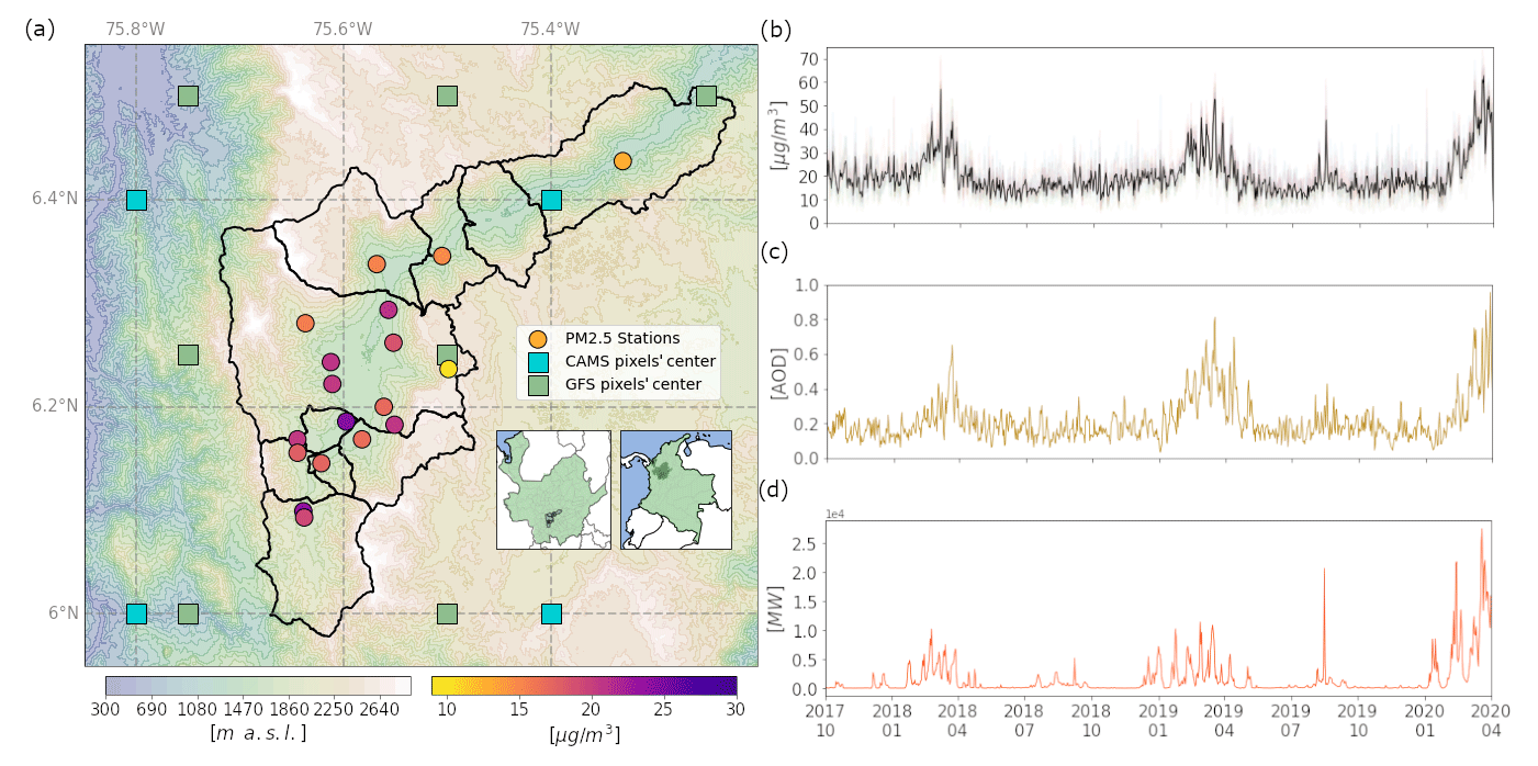
Figure 1 (a) Geographical location and digital elevation model of the Aburrá Valley. Filled circles indicate the location of the PM_2.5 stations used in this study, and their color represents the average concentration during the training period. Green and blue squares indicate the location of the GFS and CAMS pixels' center, respectively. (b) Daily-averaged time series of the mean PM_2.5 concentration from all the stations during the training period; the black line represents the average concentration in the city. (c) Same as (b) but for the total aerosol optical depth (AOD) most recent forecast from CAMS. (d) Same as (b) but for the integrated fire radiative power (IFRP) within a radius of 50 km around the 800 hPa 4 d back-trajectory from GFS.

Several elements must be considered to accurately forecast the air quality conditions a few days in advance. As for the aerosol sources, the two most relevant ones in terms of PM_2.5 are the urban emissions, mainly resulting from car engines and industrial activity (Herrera-Mejía and Hoyos, 2019), and external biomass burning aerosols from wildfires that occur in northern Colombia, the Orinoco River basin, and, with less impact in terms of local concentrations, in the Amazon River basin (Rincón-Riveros et al., 2020; Hernandez et al., 2019; Mendez-Espinosa et al., 2019; Ballesteros-González et al., 2020; Rodriguez-Gomez et al., 2022). Apart from the emissions, meteorological factors play a crucial role in reducing aerosols concentrations in the valley in two ways: the lifting and subsequent horizontal transport away from the valley of the pollutants, which occurs in response to a thermally unstable lower atmosphere, and wet deposition. Several studies have addressed the relationships between meteorological and air quality conditions in the area of interest during recent years (Isaza Uribe, 2020; Herrera-Mejía and Hoyos, 2019; Hoyos et al., 2020; Roldán-Henao et al., 2020).

Atmospheric stability plays a crucial role (Herrera-Mejía and Hoyos, 2019). Shallow boundary layers that inhibit pollutants' vertical dispersion respond to a relatively low inflow of solar radiation at the surface (Herrera-Mejía and Hoyos, 2019), primarily a product of regional cloudiness and aerosols' radiative forcing (Dubovik et al., 2002; Bond et al., 2013). Also, the dual net effect of rainfall events over the PM_2.5 concentration must be considered. Roldán-Henao et al. (2020) argue that commonly, afternoon rainfall events have a net detrimental effect on air quality; the contribution to near-surface cooling and the consequent stabilization of the lowest part of the troposphere end up being more relevant than the favorable aerosol reduction due to scavenging. On the other hand, due to their long duration and extensive coverage over the region, nocturnal rainfall events significantly contribute to reducing PM_2.5 concentrations, thanks to efficient wet deposition (Guo et al., 2014).

Even though it is impossible to have a perfectly accurate model due to the non-linearity of the relationships with the processes and variables responsible for its fluctuations, the mixed natural and anthropogenic origin of its variability, and the chaotic nature of weather phenomena (Lorenz, 1969), a forecasting model for the 24 h PM_2.5 concentration in the Aburrá Valley is pivotal in supporting decision-makers, especially during periods with high loads of aerosols. The use of ML methods in geosciences is becoming more common every day; their ability to be as accurate as numerical models without the need to know the analytical description of the relations among variables has resulted in several studies applying artificial intelligence (AI), not only for weather applications but also for pollutants' concentration prediction and diagnosis (Wang et al., 2017; Mao et al., 2017; Xu et al., 2020; Lin et al., 2021; Guo et al., 2021; Yang et al., 2021; Lv et al., 2021; Chellali et al., 2016; Perez and Gramsch, 2016; Yang et al., 2020; Perišić et al., 2017; Tian and Chen, 2010).

According to Lee et al. (2020), tree-based algorithms tend to present the best accuracy when trying to predict PM_2.5 concentrations; they propose a gradient boosting (GB) approach for predicting PM_2.5 concentration in Taiwan and London. Mao et al. (2017) use aerosol optical depth (AOD), back trajectories, and a multi-layer perceptron (MLP) model for forecasting concentrations 3 d in advance in eastern China, while Wang et al. (2017) perform a hybrid forecasting model including support vector regression (SVR) for a 10 d hourly forecast in the same region. Lv et al. (2021) compare the results from a random forest (RF) (Breiman, 2001) and an SVR method with a multiple linear regression (MLR), and they both present a significant relative improvement. Most recently, Ke et al. (2022) developed an automated air quality forecasting system that includes results from MLR, MLP, RF, GB, and SVR; they also include real-time Global Forecasting System (GFS) meteorological forecasts and use stacked generalization (SG) to get a final output from the ensemble.

Considering the advances mentioned above, this study proposes an approach for tackling the challenge of combining and exploiting diverse sources of available and valuable information to forecast PM_2.5 in a densely populated region. We use data from the monitoring network of the Early Warning System of the Aburrá Valley (SIATA), CAMS (Benedetti et al., 2009; Inness et al., 2019) and GFS (National Centers for Environmental Prediction, National Weather Service, NOAA, U.S. Department of Commerce, 2015) atmospheric forecasting models, and the MODIS active fire products (Justice et al., 2002; Giglio et al., 2003, 2016) to develop a forecast for the 24 h averaged PM_2.5 concentration in the following 4 d. One of the novelties of this study is the development of a new index used as input for the models, which is based on the satellite-derived fire radiative power within an area determined by low-tropospheric back-trajectories (see Sect. 2.4). This index ends up being crucial for the prediction of detrimental air quality events within the city. We include recent software developments (piecewise linear regression trees and a customized loss function; see Sect. 3) to improve one of the most significant downsides of tree-based models, the low performance of tree-based models over data out of the training domain, and compare the results with an MLR method. Finally, we use eXplainable AI (XAI) methods to learn more about the predictability of the PM_2.5 concentration within a narrow valley. Section 2 describes the collected data and input variables. Section 3 details the models and the fitting and testing process. In Sect. 4, we show the performance of the models, some examples, and a variable importance analysis. Section 5 presents the conclusions and discussion.

2 Data

One of the possibilities that tree-based algorithms allow is to integrate multiple sources of information and a high number of input variables straightforwardly. We use the following information sources to account for the main forcings of the PM_2.5 concentration variability (anthropogenic activity, external sources, and meteorology).

2.1 PM_2.5 monitoring network

We employ in situ hourly observations of PM_2.5 concentration from the SIATA official monitoring network; 6 BAM1020 and 13 BAM1022 devices by Met One Instruments, Inc. are distributed throughout the Aburrá Valley. The devices measure airborne particulate concentration levels using the principle of beta ray attenuation with methods endorsed by the US Environmental Protection Agency (EPA) and hold international accreditation. Of the 19 stations, 2 are located near roadways: SUR-TRAF and CEN-TRAF.

Most of the stations were installed in October 2017, with continuous measurements of hourly PM_2.5 concentrations since then. Therefore, we count with 3 years of continuous measurements to train the models. The target of the models is to predict 24 h averaged PM_2.5 concentrations, which is aligned with the standard that regulates this pollutant in Colombia and thus supports decision-making. A 24 h rolling window is applied to the concentrations, allowing an hourly assessment of the results.

2.2 AOD from CAMS

To predict episodes in which long-range transport of aerosols affects the air quality in the region of interest, we include the CAMS global atmospheric composition forecast. This model operates twice a day, at 00:00 and 12:00 UTC (https://confluence.ecmwf.int, last access: 14 December 2023), and data for the next 5 d are publicly available around 10 h after the initial run. The model counts with a horizontal resolution of approximately 40 km, and it consists of 56 chemical species of reactive traces gases in the troposphere, stratospheric ozone, and seven different aerosol types. For this analysis, we include the forecasted AOD out to 96 h lead time.

2.3 GFS

To account for the fluctuations of PM_2.5 concentrations due to meteorological changes, we use outputs from GFS from the National Center for Environmental Predictions (NCEP). This weather model produces forecasts four times a day (00:00, 06:00, 12:00, and 18:00 UTC). It predicts 16 d in advance, with a temporal resolution of 3 h; the horizontal resolution is approximately 28 km; and it has 64 layers in the vertical. In the models developed here, we include data for total cloud cover (TCC), precipitation (TP), and planetary boundary layer height (PBLH).

2.4 MODIS active fire data

The occurrence of fires, commonly related to agricultural activities (Rodriguez-Gomez et al., 2022), causes recurrent increments of PM_2.5 in the city. Figure 2 shows the correlation coefficient between the daily time series of integrated fire radiative power (IFRP) over 1^∘ × 1^∘ pixels obtained from the MODIS active fire database and the average PM_2.5 concentration at the valley, the stippling indicates areas where the correlation is statistically significant, based on a p value less than 0.025. We found high correlation coefficients over the Magdalena Basin, northeast of the city, and, more remotely, around the Orinoco Basin, in eastern Colombia and northern Venezuela.

Given that the area of interest to predict PM_2.5 depends on the wind field, we develop an approach using back-trajectories (BTs) in conjunction with the MODIS active fire data, acquired in near real time from https://firms.modaps.eosdis.nasa.gov/active_fire/ (last access: 14 December 2023) (documentation available at https://www.earthdata.nasa.gov/learn/find-data/near-real-time/firms/mcd14dl-nrt, last access: 14 December 2023); we compute the IFRP over a buffer of 50 km around a 4 d BT at 800 hPa (near-surface at the valley). The BT approach has been widely used for analysis and forecasting pollution over several places (Cobourn, 2010; Schneider et al., 2021; Wang et al., 2018; Liao et al., 2017; Louie et al., 2005) during recent years. The wind fields for the BT calculation are extracted from the GFS forecasts, and with forecast purposes, we use different wind fields for each future lead time but maintain the hotspots the same; a more detailed description of this process is presented in Appendix A. Figure 1d shows the daily-averaged time series of BT-based IFRP; the correlation coefficient with the time series of PM_2.5 is 0.59 (p value <0.025), and good correspondence is found between the seasonal peaks and some high concentration events with the IFRP.

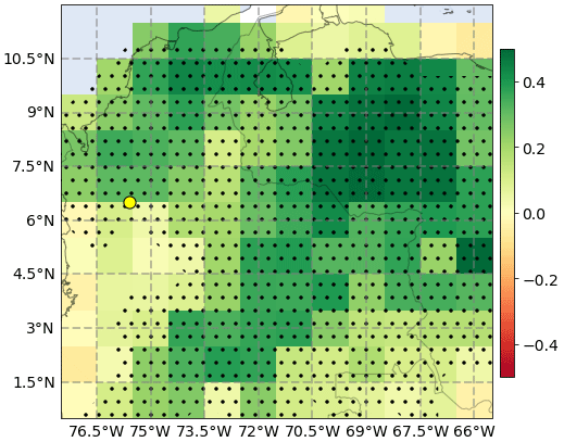
Figure 2 Spearman's correlation coefficient between the daily time series of daily PM_2.5 concentration in the Aburrá Valley and the daily cumulative IFRP over 1^∘ × 1^∘ pixels from the Aqua satellite (MODIS). The yellow point indicates the location of the Aburrá Valley, and the stippled areas indicate where the correlation is statistically significant, based on a p value less than 0.025.

3 Models

One of the challenges when forecasting is to deal with large amounts of data from different sources. Tree-based models, apart from commonly providing accurate forecasts (Kang et al., 2018), allow the inclusion and relatively fast processing of a high number of input variables, which is convenient due to all the factors that affect the air quality within the region of interest. Decision trees (DTs) are the base method used in this study. In DTs, each tree branch node represents a choice between several alternatives, and each leaf node represents a decision (Kang et al., 2018; Quinlan, 1986). The RF and GB methods are sophisticated ways of implementing DTs. On the one hand, random forest performs by using bootstrap samples of the training data and random feature selection in tree induction, and prediction is achieved by averaging the predictions of each tree within the ensemble (Cutler et al., 2012). Alternatively, gradient boosting, or greedy function approximation, uses fitting functions, loss functions, and gradient descent analysis (Friedman, 2001). GB uses the negative gradient of the loss function as the residual approximation in the fitting tree algorithm and minimizes the loss function by reducing the residual value gradually (Zhang et al., 2021).

The main downside of using tree-based models is their low capacity to make predictions outside the domain in which they were trained (Meyer and Pebesma, 2021). To address that problem, we use the algorithm developed by Tao et al. (2021) and implemented within the LightGBM Python library (Ke et al., 2017). They modify the GB method to use piecewise linear regression trees (PL trees) as base learners. This modification allows the models to capture linear relationships and to extrapolate out of the domain in which the models were trained. In addition to the LightGBM library, the Sklearn Python package (Pedregosa et al., 2011) is used for training the RF models.

One relevant issue faced when aiming to predict pollutant concentrations in cities is that decision-makers and the general public are mainly interested in the forecast of cases in which concentrations of PM_2.5 are abnormally high or low. Given that the distribution of the target values for training is highly imbalanced, we modify the classic mean squared error (MSE) loss function by weighting the loss values based on the density within the probability distribution of the target concentrations (Steininger et al., 2021). As shown in Fig. 3, the error is multiplied by a penalty value that amplifies similarly to the target values located away from the mean.

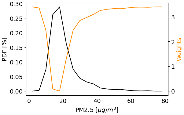
Figure 3 Probability distribution function of the 24 h averaged PM_2.5 concentrations at the station MED-LAYE (black line) and the weights associated with each bin that are used to modify the loss function for training the models (orange line).

Taking into account the data described above, the models include a total of 269 input variables that include the past 48 h PM_2.5 concentration at the station; CAMS-predicted aerosol optical depth; GFS-predicted total cloud cover, precipitation rate, and boundary layer height; predicted IFRP; day of the week; and hour of the day. The training and validation of the models go from 1 October 2017 to 20 April 2020, and their testing took place from 1 February 2021 to 31 April 2021; the period between 20 April 2020 and 1 February 2021, was excluded from the training, given the anomalous variability and abrupt changes in the emissions due to the COVID-19 pandemic. However, a brief assessment of the performance during COVID is provided in Appendix B. Before training the models, all the inputs for the different ML methods were standardized by removing the median and scaling according to the interquartile range (sklearn.preprocessing.RobustScaler(), https://scikit-learn.org/stable/modules/generated/sklearn.preprocessing.RobustScaler.html#sklearn.preprocessing.RobustScaler.transform, last access: 14 December 2023). Considering that the models run operationally and the wide variety of data sources that we use for running the models, it is possible for some input variables to not be available in real time during the operation. In these cases, the missing data points are replaced by zeroes, which would be equivalent to using the median value of the variable during the training period.

The algorithms used have relatively low computational costs. The models were trained by a computer with an 8-core CPU and 16 GB of RAM. With this architecture, the models for all stations took around 4 h to be trained. However, once trained, these models allow PM_2.5 predictions 4 d ahead in just 20 min. That includes pre-processing of the input information, generation of predictions, and post-processing.

3.1 Direct multi-output and recursive schemes

In this study, we approach the problem of having multiple outputs in two ways. On the one hand, we use the direct multi-output strategy (MO), in which we train independent models to predict each of the 96 lead time hours. On the other hand, aiming to exploit dependencies among the target values to improve the skill of the models, we try a recursive scheme (RC) (Spyromitros-Xioufis et al., 2016); in this case, each model, except for the first hour of the forecast, also depends on the predicted 24 h averaged concentration before the objective lead time. For example, the predicted values for the lead times 1 and 2 are input variables for the third forecasted hour.

3.2 Hyperparameter selection

We performed a hyperparameter grid search with a 5-fold validation during the first period to find the optimal set (Ke et al., 2022). The final choice was based on the average root mean squared error (RMSE) of the 96 predicted hours. Table C1 shows the possible values tried for every hyperparameter. The selected set of hyperparameters for a model that predicts the mean 24 h PM_2.5 concentration in the city is highlighted.

4 Results

We use the root mean squared error (RMSE), the correlation coefficient, and the mean absolute percentage error (MAPE) as evaluation metrics for the trained models; the RMSE and MAPE computation includes multiplying by the weight values described in Sect. 3 and shown in Fig. 3. The RMSE penalizes large errors more, which is relevant due to the additional importance given to cases with high concentrations. The correlation coefficient indicates covariance between the predicted and true values, and the MAPE allows a fair comparison among different stations. Figure 4a and b show the RMSE and correlation coefficient averaged over all stations for each lead time for the four developed models, and a fifth one with the same input variables but using linear regression (LR), the emergence of collinearity, due to the high number of inputs (Gregorich et al., 2021), was addressed in the LR by implementing L2 regularization (ridge regression; McDonald, 2009). According to Fig. 4a, b, GB outperforms LR at all lead times, and GB presents lower RMSE and higher correlation coefficients than RF before hour 24. Although the performance of RF is similar to GB after day 1, it performs worse than LR and GB before the first 8 forecasted hours. GB–MO has the best performance for most lead times and stations. The RMSE for GB–MO goes from 1.3 to around 7 µg m⁻³ during the 96 h lead time, and the correlation goes from 1 to 0.3. Although average correlation coefficients are low (below 0.5) after 2 d of forecast, the performance of the trained models is still better than the original CAMS PM_2.5 forecast, which presents correlation coefficients lower than 0.3 and RMSEs higher than 9 µg m⁻³ starting from day 0 for most of the stations. Following these results, GB–MO will be used for the rest of the paper.

According to Figs. 4a and c and 8, most of the system's memory attributable to past PM_2.5 concentrations is lost by around 24 h. The relatively low MAPE in the first 24 h could be a consequence of the use of PM_2.5 observations in forecasts, which greatly improve the results near initialization, but their influence falls as the lead time increases (see Fig. 8). After the first 24 h, other input variables like IFRP and AOD from CAMS contribute the most to the predictability. For the first lead times, MAPE varies between 8 % and 12 % among stations. After hour 24, it ranges from 18 % to 40 %. Overall, the best performance is achieved over stations EST-HOSP, MED-ALTA, ITA-CJUS, ITA-CONC, ENV-HOSP, and MED-TESO, located south of the valley. The stations that show the worst performance are SUR-TRAF and CEN-TRAF, two stations in which traffic is highly relevant, and CAL-JOAR, MED-BEME, and COP-CVID. According to Hernández et al. (2022), small-scale urban dynamics can significantly affect the representation of wind and temperature regimes in the center of the valley and to the north, where the valley is also narrower and global models such as GFS and CAMS may have a worse performance. A poor representation of these features may explain the spatial differences in error; however, a deeper analysis of the particularities of each station is necessary to assess the causes of the higher errors. Small-scale dynamics or emissions may also cause a reduction in the models' performance.

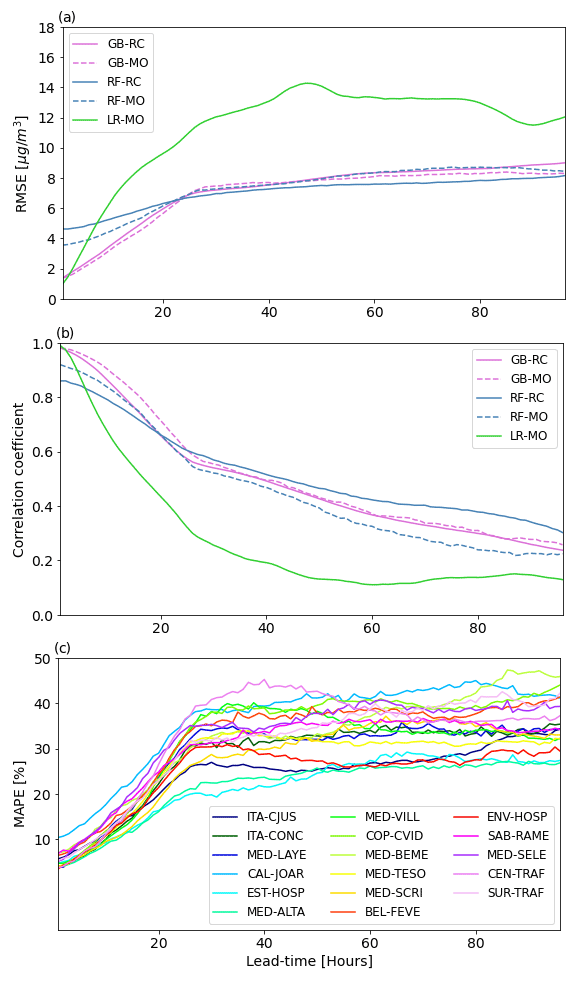
Figure 4 (a) RMSE at different lead times for the four developed tree-based models and for a fifth one with the same input variables but with a linear regression. (b) Same as (a) but for the correlation coefficient. (c) Shows the MAPE for the GB–MO model at all the stations of interest.

Figure 5 shows the scatter plots between the predicted and observed 24 h averaged PM_2.5 concentration for lead times of 1, 12, 24, and 48 h at the stations MED-SELE, MED-LAYE, and SUR-TRAF. Thanks to the customized loss function and the inclusion of the PL trees as base learners, the models accurately represent concentrations that are significantly separated from the mean. Comparisons were made with a model trained with MSE as a loss function and traditional GB (without the PL trees; not shown), and the conventional model struggled to predict high or low concentrations relative to the mean, even from the first lead times of forecast. One of the limitations of the models is that, after hour 24, they exhibit a positive bias (see Fig. 5 at hours 24 and 48), and, as expected, the representation of events with significantly high or low concentrations gets worse. One of the reasons for the inadequate estimation of these events could be the lack of those values during the training period. Additionally, although the modifications to the loss function and the GB method helped, the inability of tree-based models to extrapolate is a vulnerability for the long-term sustainability of this strategy. However, given the low computational power needed, the models can be re-fitted frequently (e.g., monthly or every 3 months) as more data are available. Other sources of error include the initial and boundary conditions used for CAMS and GFS, which are later used as inputs in our models. The use of other model architectures, or the improvement of the inputs representing the meteorology in the region by implementing high-resolution numerical modeling, could complement these results and lead to a more robust and reliable forecast, especially given the high number of new regulations and governmental decisions that could influence air quality in urban areas.

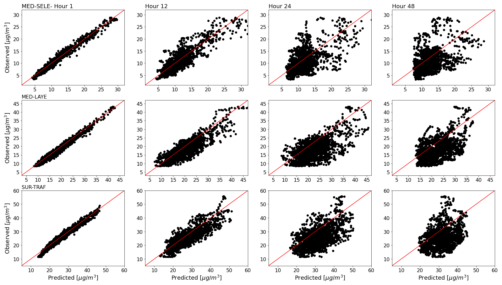
Figure 5 Scatter plots between the observed and predicted 24 h averaged PM_2.5 concentration at three different stations (MED-SELE, MED-LAYE, SUR-TRAF) and four different lead times (1, 12, 24, and 48 h.)

Despite these performance limitations, the model is still helpful for decision-makers in the city. During the testing period, the night of the 6 March and early morning of 7 March presented an event with generalized poor conditions in terms of air quality over the metropolitan area of the Aburrá Valley. Two population-representative stations presenting the worse concentrations were CAL-JOAR and ITA-CJUS. Figure 6 shows a sudden increment in the 24 h average concentration at both stations of around 15 µg m⁻³, leading to unhealthy conditions for sensitive groups over a prolonged time. The sudden increment was observable in the two stations' forecasts more than 24 h in advance (see blue lines in Fig. 6). To check the relevance of some variables for predicting this event, we trained the same model but excluded one of the inputs each time. AODs from CAMS and BT-IFRP were crucial to simulate the high concentrations in advance; in the tests excluding them (see green and orange lines in Fig. 6), the models did not capture the high magnitude of the peak.

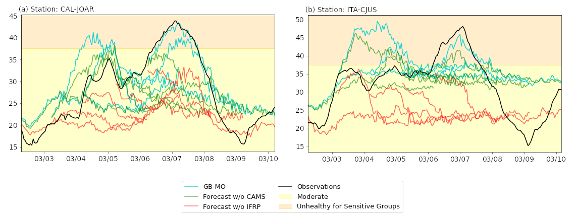
Figure 6 Observed 24 h averaged PM_2.5 concentration at the stations CAL-JOAR and ITA-CJUS (black line) and forecasts every 24 h before the peak concentration on 21 March 2021 at 06:00 UTC−5. The green and red lines indicate the forecast without considering CAMS and the IFRP index, respectively. The background colors indicate the corresponding air quality index (AQI) levels of concern.

Figure 7 shows how the error (MAPE and RMSE) varies during the day for different lead times. While there are no marked differences among different hours of the day for the first 12 h within the forecast range, a gradient in error starts developing in the early morning at a lead time of around 18 h, with a peak in error that starts in the early morning and shifts towards the afternoon as the lead time increases. The gradient becomes the sharpest at around 30 h. This pattern repeats again for the third, fourth, and fifth days of forecasts, but for these days, the peak in error presents at around 10:00. After noon, the error decreases slightly again in the hour-of-the-day dimension. As recent studies about air quality in the Aburrá Valley mentioned (Herrera-Mejía and Hoyos, 2019; Hoyos et al., 2020; Roldán-Henao et al., 2020), one of the most significant sources of uncertainty is the time of the boundary layer's expansion, which is also closely related to the turbulent processes occurring near the surface. Compared to global models (like GFS), regional models such as the Weather Research and Forecasting (WRF) model have proven a better performance in representing localized meteorological conditions (Posada-Marín et al., 2019; Gutowski et al., 2020). This is especially important in complex terrain regions such as the Aburrá Valley (Henao et al., 2020). Thus, the improvement in the representation of dynamics and thermodynamics by WRF simulations could provide a better representation of small-scale processes responsible for the intra-diurnal variability of the PM_2.5 concentration and improve air quality forecasts in the region.

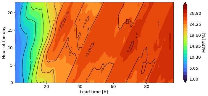
Figure 7 MAPE (filled contours) and RMSE (black contours) for the different lead times at different hours during the day averaged over all stations.

4.1 Variable importance

Aiming to have a better understanding of the sources of predictability and uncertainty for the forecasts, we use two complementary approaches to analyze the variables' importance: (i) the intrinsic method from GB or the mean decrease in the loss function (MDLF). This method quantifies feature importance based on the improvement in the loss function contributed by each feature across all splits in the tree (Ke et al., 2017). (ii) We also perform a permutation feature importance analysis, which measures how much the forecast error increases when randomly modifying each input variable. For the second approach, we repeated the computation 10 times during the evaluation period for each variable in order to get more robustness. The MDLF approach is computationally efficient, but it suffers from biases, especially when the cardinality of the input variables is high (Lundberg et al., 2018). On the other hand, despite the permutation importance method being generally accepted as reliable (Loecher, 2022), it is significantly more computationally expensive than the MDLF approach. Both methods struggle when dealing with input variables that are correlated among them; however, we performed the same analyses using principal component analysis to reduce the dimensionality of the inputs, and the features' importance remained the same.

Given the high number of inputs and stations, we summed the values corresponding to eight different macro-variables for each lead time: past PM_2.5 concentrations, AOD, TCC, precipitation rate (PRATE), height of the PBL (HPBL), IFRP, day of the week, and hour of the day. Figure 8a and d show the importance of each category from the two mentioned methods averaged over all stations. As expected, both methods agree that the relevance of past concentrations is maximum during the first hours of the forecast and decreases quickly until around the 30th hour. Also, the relevance of CAMS AOD increases with time, and it becomes the most important variable at around the 40th hour. Apart from those two variables, both methods coincide in that the BT-based IFRP index is the most useful variable between the 20th and the 40th hour of the forecast.

Relative to the past concentrations, CAMS AOD, and IFRP, the importance of the other variables considered in this study is significantly lower. The relative magnitude of the importance of these other variables depends on the station, and there is a high level of agreement between the two methods. The analyses show that precipitation from GFS is significantly relevant after the 20th hour of the forecast for stations ITA-CONC, CAL-JOAR, EST-HOSP, MED-ALTA (see Fig. 8b), MED-VILL, MED-SCRI, CEN-TRAF, and SUR-TRAF. Similarly, planetary boundary layer height is relevant for stations CEN-TRAF, MED-ARAN, MED-TESO, MED-BEME, MED-VILL, and ITA-CJUS. Cloud cover was shown to be relevant after the 60th hour of the forecast for stations MED-LAYE, COP-CVID, MED-TESO, and MED-SELE (see Fig.  8c). Finally, the day of the week showed high importance in ITA-CJUS, MED-ALTA, MED-BEME, CEN-TRAF, and SUR-TRAF. These results correspond with the environmental characteristics and location of each station. In MED-SELE (Fig. 8c), the variables that affect the near-surface concentration at the base of the valley, such as HPBL or PRATE, are not as important, which is consistent with MED-SELE being significantly higher than the rest of stations. For SUR-TRAF and CEN-TRAF, whose variability is dominated mainly by vehicular emissions, and for other stations near the region's urban and commercial center, the day of the week showed predominance in the lead times after day 2.

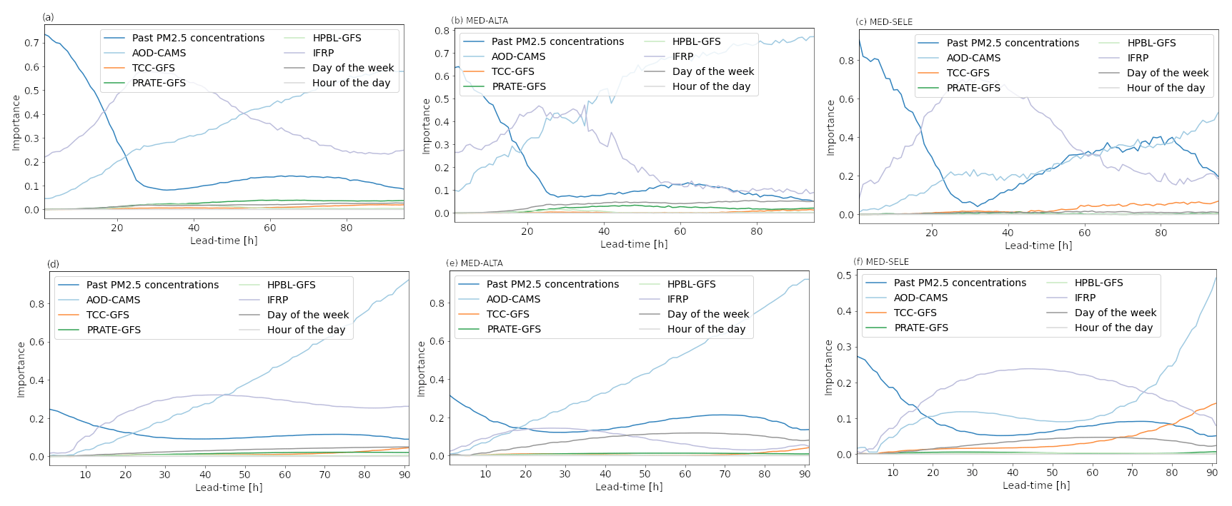
Figure 8 MDLF (a–c) and permutation (d–f) feature importance for the different groups of variables and lead times included in the forecast. Panels (a) and (d) show the feature importance when averaged for all stations. Panels (b) and (e) and (c) and (f) show the feature importance for stations MED-ALTA and MED-SELE, respectively.

5 Conclusions

Given the negative effects of poor-air-quality episodes in highly populated areas, forecasting PM_2.5 concentrations is paramount for decision-makers in cities, especially in developing countries like Colombia. In this study, we developed a framework for forecasting 24 h averaged PM_2.5 concentrations in the Aburrá Valley. In order to exploit the variety of useful information sources available, we combine tree-based machine learning algorithms with multiple data sources that are accessible in real time. Along the process, we developed a novel input variable for the models based on the radiative characteristics of fires occurring within an area of interest indicated by back-trajectories. Finally, we included a feature importance analysis that contributes to the understanding of the uncertainties and physical processes influencing short-term predictability over a complex terrain and densely populated region.

Both RF and GB performed significantly better than linear regression. However, the GB–MO strategy presented the best performance at almost all stations. The models were able to predict the episode with the poorest air quality during the testing period with more than a day of anticipation. Additionally, while one of the main limitations of tree-based methods is the low skill when dealing with predictions out of the domain of the training dataset, using a density-weighted loss function and implementing piecewise linear regression trees as base learners for the GB method helped overcome the issue.

According to the feature importance analysis, both the identification of external sources, such as wildfires, and local meteorological changes, especially those related to the boundary layer, proved to be relevant in predicting the occurrence of poor-air-quality events and the intra-diurnal changes in PM_2.5 concentration, respectively. The BT-based IFRP approach accomplished the objective of including near-real-time observations in the forecast and adding predictability by complementing the CAMS forecast. There is room for improvement regarding the precision of the fires' intensity, the error in the predicted wind fields, and the temporal evolution of fires.

Future work on the forecasts should be mainly focused on improving the representation of the diurnal variability within the models and reducing the biases after the first day within the lead times. A better understanding of the boundary layer processes in the urban area and the inclusion of more detailed meteorological forecasts could lead to performance improvements, mainly in the morning hours. An inadequate representation of the boundary layer could lead to false alarms when underestimating the expansion of the boundary layer and to missing high concentrations when overestimating it. Another factor that should be considered in the future is the formation of secondary particulate matter. Apart from the inclusion of PM_2.5 precursors that could lead to better accuracy, studies in the region that identify and characterize those compounds are also needed.

ML models show great potential to simplify, integrate, and apply large amounts of information for forecasting air quality conditions, which ultimately ends up as an excellent tool for decision-makers in the city. Furthermore, the knowledge acquired in the SIATA monitoring network during the past few years was vital to selecting the correct inputs and looking at the most conducive variables. In addition, without maintaining the records that span several years at the studied PM_2.5 stations, models' robustness would not have been possible, which motivates continued data collection at the respective locations.

Appendix A: Back-trajectory (BT) methodology for the BT-based integrated radiative power (IFRP)

Lagrangian analyses, and specifically back-trajectories, help analyze the origin of pollutants spatially, mainly regional long-range transport (Cobourn, 2010; Schneider et al., 2021; Wang et al., 2018; Liao et al., 2017; Louie et al., 2005). In the case of the Aburrá Valley, as shown in Sect. 2, fires occurring hundreds of kilometers away from the city have a significant and recurrent impact over the PM_2.5 concentration in the stations of interest.

The BT tracking is based on sequentially computing the past position of the parcel of air of interest in a given past time. The past coordinates of the parcel are computed as

$$\begin{array}{}\text{(A1)}& \mathit{X}(t-\mathrm{\Delta }t)=\mathit{X}\left(t\right)-\mathit{V}(\mathit{X},t-\mathrm{\Delta }t)\cdot \mathrm{\Delta }t,\end{array}$$

where X is the 3D spatial location of the parcel, t is the current time, Δt is the time step, and $\mathit{V}(\mathit{X},t-\mathrm{\Delta }t)$ is the wind speed in the three directions.

In our case, the ending point of the parcels – or position at the time of interest (t_f) – is located horizontally near the valley's center and at a pressure slightly lower than the average of the region's surface, that is, longitude, latitude, and pressure of

$$\begin{array}{}\text{(A2)}& \mathit{X}\left(t_{\mathrm{f}}\right)=\left[\begin{array}{c}\mathrm{75}{}^{\circ }\mathrm{W}\\ \mathrm{6.25}{}^{\circ }\mathrm{N}\\ \mathrm{800}\mathrm{hPa}\end{array}\right].\end{array}$$

The algorithm computes the parcel's position 4 d back in time at a temporal resolution (Δt) of 1 h, and the forecasted wind fields for the trajectory calculation are extracted from the latest available GFS forecast.

After computing the BTs corresponding to parcels arriving at the valley at different lead times, we create a buffer of 50 km around the obtained trajectory. Finally, we integrate the radiative power of the fires located within the buffer to get the BT-IFRP index used as input for forecasting PM_2.5 concentrations.

Appendix B: Performance of the models during the COVID period

In order to further elucidate the models' limitations, we selected two additional evaluation periods: (i) a 10 d period during the COVID-19 pandemic, from 20 to 30 April 2020, for a comparison with the same 10 d of the test period in 2021, and (ii) a 30 d period (from 20 April to 20 May 2020) to get more robust statistics. On average, the 24 h PM_2.5 concentration for the 10 d test period during the pandemic is 3.7 µg m⁻³ lower than the corresponding 10 d within the study's test period (20 to 30 April 2021), which corresponds to a difference of around 20 %. Due to these differences, we used MAPE as the evaluation metric. Figure B1 shows that errors during the pandemic are comparable to those in the 2021 testing period and even lower for lead times of more than 24 h. Additionally, correlation coefficients are also comparable between the two periods (see Appendix Table B1).

Altogether, these results highlight the ability of the forecasts to generalize the predictions under different conditions. Nonetheless, future studies can perform longer training of the models, including data from subsequent years, which could result in an improvement of the forecast’s skill.

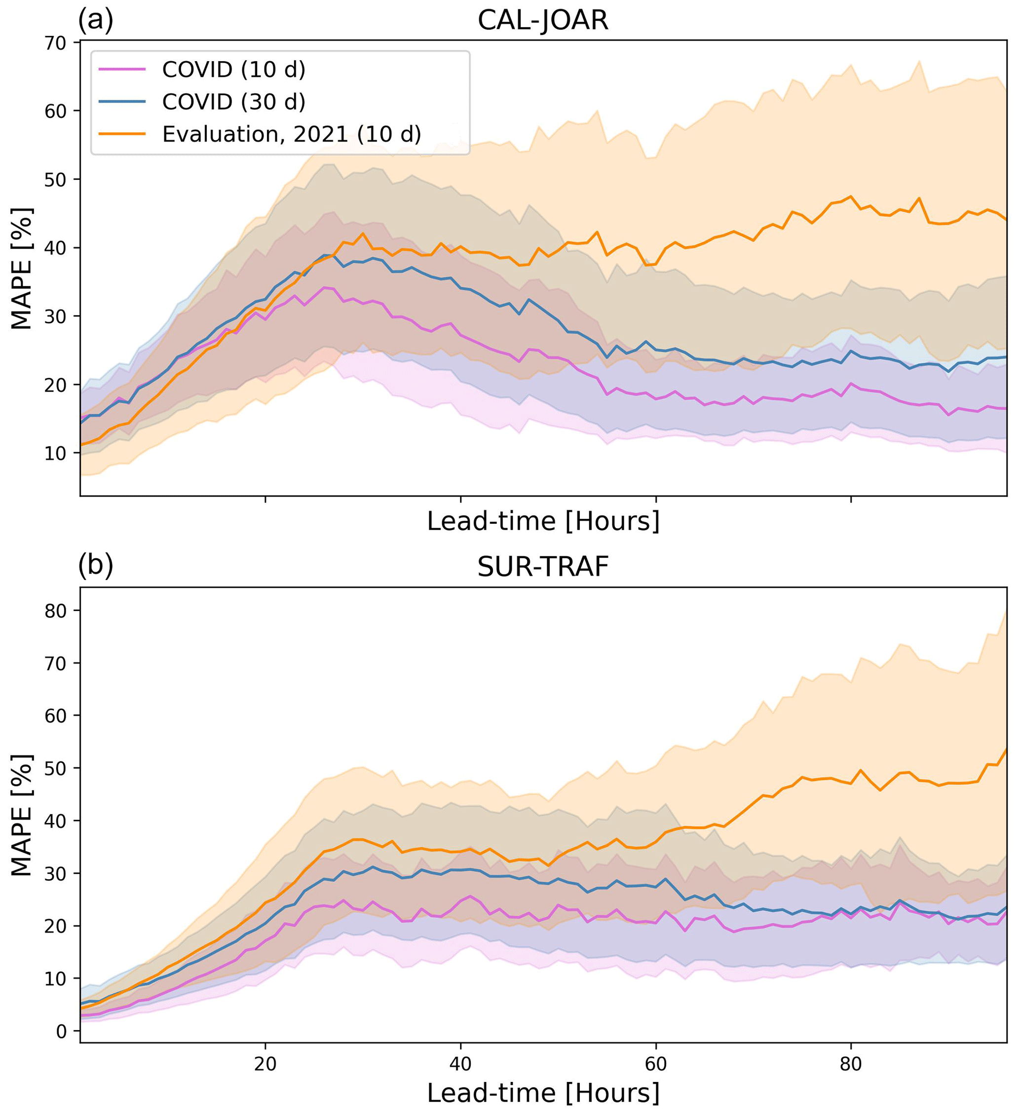
Figure B1 Mean absolute percentage error (MAPE) as a function of lead time for 10 d of the validation period (orange), the corresponding 10 d during the COVID pandemic (magenta), and the 30 d COVID evaluation period (blue). Panel (a) shows the results for the CAL-JOAR station, while panel (b) is for the SUR-TRAF station. Shading represents 1 standard deviation error.

Table B1 Pearson correlation coefficient computed for the different testing periods: the 10 d from 2021 (Eval10d), the 10 d from 2020 (COV10d), and the 30 d from 2020 (COV30d). The metric was calculated as a function of lead time (hours 12 and 24) and for different stations.

Appendix C: The explored set of hyperparameters

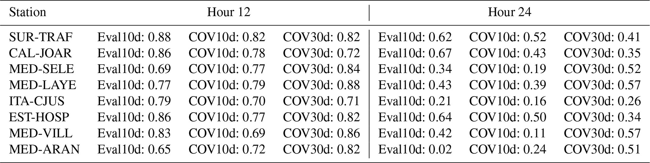
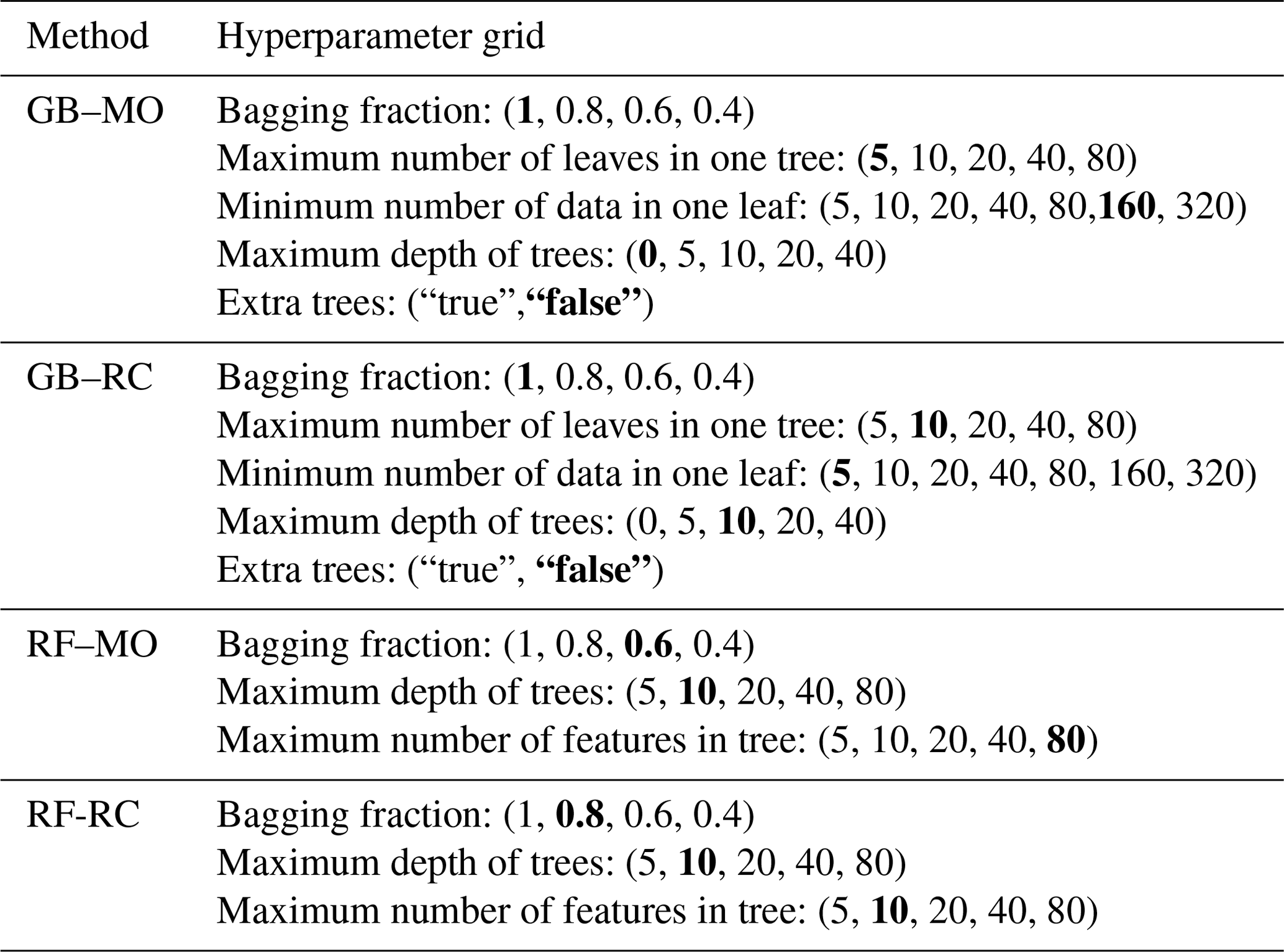
Table C1 shows the hyperparameters explored during the optimization process. The selected set of hyperparameters for each model is highlighted.

Table C1 Grid of hyperparameters used in the hyperparameter optimization process. The best options based on the output average error in the 96 h of the forecast are in bold.