the Creative Commons Attribution 4.0 License.
the Creative Commons Attribution 4.0 License.
 | 24 May 2023
Changes in the distribution of annual maximum temperatures in Europe
Gabriele C. Hegerl
Ioannis Papastathopoulos
In this study we detect and quantify changes in the distribution of the annual maximum daily maximum temperature (TXx) in a large observation-based gridded data set of European daily temperature during the years 1950–2018. Several statistical models are considered, each of which analyses TXx using a generalized extreme-value (GEV) distribution with the GEV parameters varying smoothly over space. In contrast to several previous studies which fit independent GEV models at the grid-box level, our models pull information from neighbouring grid boxes for more efficient parameter estimation. The GEV location and scale parameters are allowed to vary in time using the log of atmospheric CO2 as a covariate. Changes are detected most strongly in the GEV location parameter, with the TXx distributions generally shifting towards hotter temperatures. Averaged across our spatial domain, the 100-year return level of TXx based on the 2018 climate is approximately 2 ∘C (95 % confidence interval of [2.03,2.12] ∘C) hotter than that based on the 1950 climate. Moreover, averaged across our spatial domain, the 100-year return level of TXx based on the 1950 climate corresponds approximately to a 6-year return level in the 2018 climate.
- Article
(4584 KB) - Full-text XML
- BibTeX
- EndNote


The greenhouse effect, whereby increasing levels of greenhouse gases in the Earth's atmosphere lead to a warming of the climate system, has long been understood (Charney et al., 1979), and in 2019, atmospheric CO2 concentrations were higher than at any time in at least 2 million years (IPCC, 2021b). Allen et al. (2018) estimate that human-induced warming in 2017 reached approximately 1 ∘C above pre-industrial levels and is increasing at a rate of approximately 0.2 ∘C per decade. Hoegh-Guldberg et al. (2018) describe the impacts of 1.5 ∘C global warming above pre-industrial levels on natural and human systems. These impacts include an increase in the frequency and intensity of heavy-precipitation events, more frequent marine heatwaves and reduced crop production and yields.
Temperature extremes, which may manifest in more intense heatwaves and enhance the risk of fires, pose a risk to human health (IPCC, 2014, Sect. 2.3.2), with the elderly being particularly vulnerable to heat-related mortality (Basu and Samet, 2002). An estimated 40 000–70 000 heat-related deaths were recorded as a result of the summer of 2003 European heatwave (Fischer and Schär, 2010; Robine et al., 2008), with associated economic losses in excess of EUR 13 billion (de Bono et al., 2004). Due to the potentially devastating consequences, it is clearly important to understand how the frequency and intensity of temperature extremes may change in a warming climate.
Several previous studies consider changes in the probability distribution of daily temperature and infer that similar changes should also hold for extremes. Donat and Alexander (2012) consider the distribution of daily maximum and minimum temperature on a global scale using observational data and find significant shifts in temperature towards higher values in almost all regions but less evidence for changes in variability. Similar conclusions are reported in Weaver et al. (2014), who analyse data from several hundred climate model runs. Schär et al. (2004) on the other hand argue that an increase in variability in the daily temperature distribution is required to explain the European heatwave of 2003.
Kiktev et al. (2003) and Morak et al. (2013) both find that there has been a decrease in the frequency of cold extremes and increase in the frequency of hot extremes, concluding that human-induced forcing has played an important role. Stott et al. (2004) consider human influence on the summer heatwave of 2003 and find that “it is very likely (confidence level >90 %) that human influence has at least doubled the risk of a heatwave exceeding this threshold magnitude”. Zwiers et al. (2011) use observational data together with climate model output in a detection and attribution study of changes in temperature extremes. They consider several variables, including annual maximum daily maximum (TXx) and minimum temperatures (TNx), and find evidence for anthropogenic forcing for all variables they consider, with the biggest changes being detected in TNx. More recently, the IPPC report (IPCC, 2021b) concluded that “human-induced climate change is the main driver” of the increase in intensity and frequency of hot extremes.
In this paper we consider statistical models for the variable TXx at approximately 12 000 locations of a gridded data set in a large subset of Europe. We consider the question of whether, over various large sub-regions of Europe, there is evidence for changes in the distributions of TXx and, if so, how such changes are best described. Our approach can, informally, be viewed as macroscopic, since we are interested in detecting changes in TXx on a large scale rather than at any one specific geographic location. We fit statistical models that allow for changes in both the location and scale of the TXx distributions. A change in the location of the TXx distribution corresponds to a horizontal shift in the distribution, with the mean and all quantiles being shifted by the same amount. A change in scale corresponds to a horizontal stretching or compression of the distribution, which in turn changes measures of variability, such as the variance of TXx. Figure 1 illustrates both of these effects for a hypothetical TXx distribution.

Figure 1The solid black curve shows a hypothetical probability density function of TXx. The dashed curve illustrates the effect of a shift in the location of the distribution towards hotter temperatures, while the dotted curve illustrates a change in the scale, leading to greater variability in TXx.
Most of the studies mentioned above treat the data occurring at different geographic locations in an independent manner, fitting separate statistical models to the data at each location. One difficulty with this approach in the context of extremes is that, as extreme observations are by definition rare, we will only have
a small sample at each location, making precise estimation of trends problematic. Although it may be unreasonable to assume a common trend at every geographic location of a large spatial domain, we would nonetheless expect nearby regions to be similarly affected by climate change. There are several classes of models, such as varying coefficient models (Hastie and Tibshirani, 1993) or geographically weighted regression models (Brunsdon et al., 1998), that allow us to borrow strength from neighbouring locations to obtain spatially coherent estimates of trends. Varying coefficient models allow for regression coefficients, e.g. trends, to vary smoothly over a spatial domain and may be formulated under the generalized additive model (GAM) framework of Wood (2017)
and consequently fit with the R (R Core Team, 2021) package mgcv.
As we work with a gridded domain, we consider a discrete analogue of varying coefficient models that are based on Gaussian Markov random fields (Rue and Held, 2005) and fall under the general smooth modelling framework of Wood et al. (2016).
Previous studies that make use of GAMs or smooth models for modelling environmental extremes include Chavez-Demoulin and Davison (2005) and Youngman (2019).
The lack of availability of high-resolution, continental-scale, temporally complete and homogenized observational data, together with the impracticality of performing large-scale controlled experiments on the climate system, means that climate researchers often rely on gridded data products (New et al., 2002). Common types of gridded data include climate model output (Eyring et al., 2016), reanalysis data (Hersbach et al., 2020) and gridded station data (Cornes et al., 2018; Dunn et al., 2020).
Gridding of station data is performed using aggregation of stations within spatial boxes, often with estimates of uncertainty. This yields estimates of area-averaged data that are comparable with climate model data over a similarly sized grid box, making them widely used for climate model evaluation (Kim et al., 2020), although they have also been used to detect past changes in mean climate and climate extremes (Haug et al., 2020; Zwiers et al., 2011). Alternatives include kriging of station data (Rohde and Hausfather, 2020), which tend to yield similar results to grid-box-averaged data over densely covered regions. Reanalysis data are data from weather analysis models that operate on grids by construction and are also often used to detect and correct biases that exist in climate models (Thorarinsdottir et al., 2020). The methodology that we develop in this paper for gridded data may be useful in other contexts and help improve the robustness of findings compared to the commonly applied independent grid-box analyses.
The structure of the paper is as follows. Section 2 describes the data that are used for fitting statistical models. Section 3 describes the models that are considered and Sect. 4 presents the results which are summarized in Sect. 5.
We use the daily E-OBS data, publicly available through the European Climate Assessment and Dataset (ECA & D) project. E-OBS is based on observational data from an underlying network of weather stations interpolated onto a regular grid. Although the data set covers all of Europe as well as northern Africa and the Middle East, the spatial density of the underlying weather station network that is used to estimate the gridded areal averages is highly variable over the domain.
E-OBS is frequently used as a benchmark at the European scale (Kotlarski et al., 2017) and was also used in the most recent IPPC report, e.g. for the atlas (IPCC, 2021a) of observed trends in temperature and precipitation. It is used in Haug et al. (2020), who also seek to provide a more rigorous methodology beyond the independent grid-box-level analyses by fitting a spatial model for trends in mean temperatures in Europe. However, they use an earlier version of E-OBS that is less suitable for detection of trends than the version we use here.
Both Hofstra et al. (2009) and Hofstra et al. (2012) express reservations about using E-OBS for the detection of trends, mainly due to inhomogeneities that may be present in the underlying station data, i.e. non-climatic factors such as changes in instruments or observing practices, as well as the fact that the network density is not homogenous in time. The documentation accompanying the release of E-OBS v18.0 also comes with a similar warning: “it remains the case that many of the input station series have not been homogenized and at present we caution against the use of E-OBS for evaluating trends” (Cornes et al., 2018). For this reason we use the E-OBS v19.0eHOM data, which are a version of E-OBS that has been homogenized by the ECA & D in collaboration with the Horizon 2020 EUSTACE project. The method by which the data were homogenized is described in Squintu et al. (2019).
In addition to inhomogeneities, a further issue with observation-based gridded data is that in regions with very low station density, grid-box areal averages may be poorly estimated and have large interpolation uncertainties. However, these problems are less severe for a spatially smooth variable such as temperature in comparison to precipitation (Doblas-Reyes et al., 2021, Sect. 10.2.2.4). As discussed in Hofstra et al. (2009), the spatial smoothness of temperature means that, although extreme-value methods have not been employed in the gridding of the daily-level E-OBS data, overall extreme temperature events will be quite well represented. Working on a much coarser grid than we do here, Zwiers et al. (2011) argue that the spatial correlation of temperature at very large distances means that even a single weather station should represent the grid-box mean extremes well. As we are interested in detection of large-scale spatially averaged changes in the distribution of TXx, issues such as poor sampling of topography in low-density regions should be less of an issue in comparison if we were seeking to quantify changes at a local level.
A plot of the station network density used in E-OBS can be found in Schrier et al. (2013), which shows that the highest density is in central Europe and that there is particularly low density in northern Africa, the Middle East and eastern Europe. The data set covers the years 1950 to 2018, with some missing data mainly in the early years, although there are also few data for Russia in the last 10 years. We consider a large subset of the full domain covered by E-OBS, shown in Fig. 2, that has reasonable station density. The values displayed in Fig. 2 are the maximum value of TXx recorded during our study period, 1950–2018. With the exception of the United Kingdom and the Republic of Ireland, islands off the mainland are excluded. We set the value of TXx at a given location in a given year as missing if there are more than 10 missing daily values in that year. This is a slightly stricter criterion than is typically applied in other studies; e.g. Zwiers et al. (2011) allow for 15 missing observations. The value of TXx in a given grid box in a given year corresponds to an extreme of a regional average which is, arguably, more useful for measuring heat risk than a local, point-wise, extreme.
For atmospheric CO2 concentration, we use data from the shared socio-economic pathway (SSP), compiled in Meinshausen et al. (2020). The historical, observation-based SSP data are only available until the year 2015, after which projections are provided until the year 2500 under different socio-economic scenarios. For the years 2016 to 2018, we took values from a mid-range scenario, namely SSP2-4.5, that are similar to the values recorded at the Mauna Loa Observatory (Keeling et al., 1976). Although the Mauna Loa data have observations available for the years 2016–2018, they have no observations during 1950–1958, so that the first 9 years of our study period are missing.

Figure 2The spatial domain considered, showing the maximum value of the variable TXx (annual maximum daily maximum temperature) at each grid box during the period 1950–2018.
3.1 Generalized extreme-value distribution
Our approach is based on fitting generalized extreme-value (GEV) distributions to the TXx values at each grid box. Another possible and theoretically well-founded approach to modelling extremes is the peaks-over-threshold method (Davison and Smith, 1990), which models the distribution of exceedances above some large threshold rather than the maximum over large blocks of observations. We prefer the block maxima approach in our setting due to the difficulty in making a principled choice of appropriate thresholds at such a large number of spatial locations as well as the sensitivity of inference to the choice of thresholds, which is exacerbated by the presence of trends (Northrop and Jonathan, 2011).
Just as variations in the mean of a large number of independent and identically distributed random variables are naturally modelled by a normal (Gaussian) random variable, variations in the sample maximum are most naturally modelled by a GEV random variable with distribution function
where , is a vector of parameters that relate to the location, scale and shape of the distribution respectively and The formal justification for using the GEV distribution to model TXx comes from the extremal types theorem (Coles, 2001, Theorem 3.1.1). The case where ξ=0 in Eq. (1) should be interpreted as the limit as ξ→0, which gives rise to the Gumbel distribution function The case ξ>0 is known as the Fréchet class of distributions and ξ<0 as the Weibull class.
The three classes () differ from each other in the behaviour in their upper (right) tail. For the Fréchet class, the right tail decays according to a power law, and for larger values of ξ, extremes take on an increasingly volatile nature, such as might be expected in financial (Resnick, 2007) or hydrological (Katz et al., 2002) applications. The Weibull class has an upper bounded right tail, with the theoretical maximum possible value, whereas the Gumbel class is an intermediate case with a light upper tail that decays exponentially. Typically, when modelling annual maximum temperatures, we expect them to be in either the Weibull or Gumbel class, i.e. ξ≤0 (Andrade et al., 2012).
Suppose that, in grid box i of the E-OBS data, we observe the annual maximum temperature in a total of ni years, say , which for most grid boxes is each year from 1950 to 2018 inclusive, so that ni=69. Let denote the annual maximum temperature in grid box i in year tij, . If we assume that are independent realizations of a GEV random variable with a distribution function as in Eq. (1) and parameters , then one way to estimate Ψi is to find the parameter configuration that maximizes the log-likelihood function l(Ψi), i.e. , where and with G as in Eq. (1), is the GEV density function. The explicit expression for the log-likelihood function is
with the case ξi=0 being defined by continuity.
Although the annual maximum temperatures may not be independent, it is assumed that the dependence between maxima from different years is sufficiently weak that
the log-likelihood in Eq. (2) may be used as a reasonable approximation of the true likelihood.
The resulting maximum-likelihood estimator is a consistent and asymptotically normal estimator of the true parameter vector provided that (Smith, 1985; Bücher and Segers, 2017). Hosking (1985) gives details for implementing the Newton–Raphson method to find the parameters Ψ that maximize Eq. (2), and several R (R Core Team, 2021) packages, e.g. ismev (Heffernan and Stephenson, 2018) or extRemes (Gilleland and Katz, 2016), provide routines for estimating the GEV parameters using maximum likelihood. The maximum-likelihood estimates of the three GEV parameters at each grid box of the E-OBS data are shown in Fig. 3, which were calculated using ismev.
Having estimated Ψi, we may estimate the temperature yp that is exceeded in grid box i in a given year with probability p by solving the equation for yp, with G as in Eq. (1). This yields the estimate of yp:
The quantity yp is known as the return level with an associated return period .
From Eq. (3) we see that errors in the estimated value of ξi may be magnified in the estimate of yp. When the sample size is small, the maximum-likelihood estimator of ξi can have a high bias, leading to absurd estimated return levels that would be deemed physically impossible, and several authors (Coles and Dixon, 1999; Martins and Steidinger, 2000) have proposed adjustments to the log-likelihood function, Eq. (2), to overcome this difficulty.
An alternative to maximum-likelihood estimation that is more robust to small sample sizes is the method of L-moments or, equivalently, probability-weighted moments (Hosking et al., 1985; Hosking, 1990). The method of L-moments is often used in a spatial setting (Kharin and Zwiers, 2005) as part of a regional frequency analysis (RFA), as set out in Hosking and Wallis (2005). In a RFA, data from different regions that are deemed to be sufficiently homogenous are pulled together to increase the sample size and hence reduce the uncertainty in parameter estimates. One difficulty with RFA is the sensitivity of the results to the method used to identify homogenous regions. Moreover, L-moment estimation is not suited to statistical modelling as it does not allow the GEV parameters to depend on the values of covariates such as the atmospheric level of CO2. Our approach, described in Sect. 3.2, has a similar motivation to RFA, but as it is likelihood-based, it allows for the inclusion of covariates.
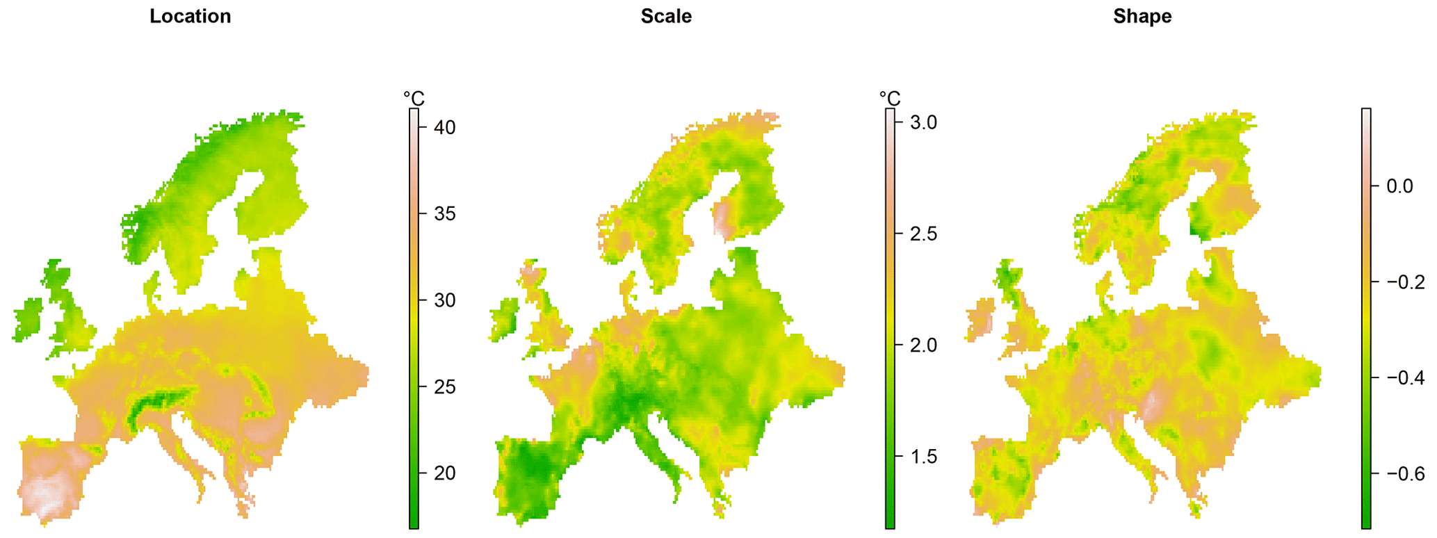
Figure 3Maximum-likelihood estimates of the GEV parameters, fitted to the TXx values (∘C) separately at each grid box.
3.2 Statistical models
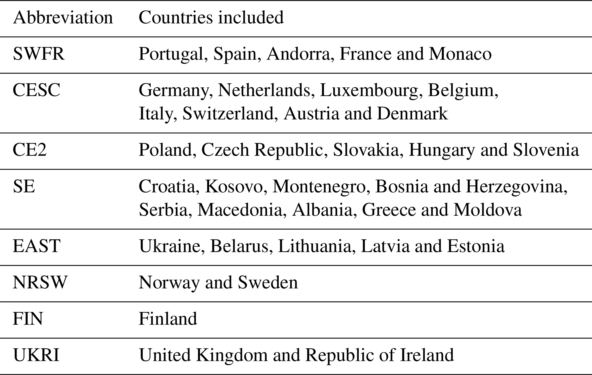
In this section we describe the statistical models that we fit to the E-OBS data. For computational convenience, and also to allow for the possibility that different models may be better suited to different regions, we partition our spatial domain into eight sub-regions, which are defined in Table 1. The abbreviations used for the regions are meant to be informative and correspond, roughly, to south-western Europe and France (SWFR), central and southern–central Europe (CESC), central Europe 2 (CE2), south-eastern Europe (SE), eastern Europe (EAST), Norway and Sweden (NRSW), Finland (FIN) and the United Kingdom and Republic of Ireland (UKRI).
Table 1The various sub-regions of the domain that the models from Table 2 are separately fitted to.
For statistical modelling of TXx, the log-likelihood function in Eq. (2) may be considered too simple in at least two respects. Firstly, it assumes that the GEV parameters at a given grid box remain fixed from year to year, whereas a potentially more realistic model would allow them to change over time. Secondly, we expect that the parameters of neighbouring grid boxes are more likely to be similar than those of grid boxes that are far apart, and Eq. (2) does not allow us to incorporate this belief. Moreover, maximizing Eq. (2) separately for each grid box i may lead to highly uncertain or unrealistic parameter estimates due to the small sample available at each grid box, and for the purposes of statistical inference, we also run into problems with multiple comparisons (Farcomeni, 2008; Chen et al., 2017).
The dependency of the GEV parameters on time can be linked to that of a climatological covariate, and for this purpose we will use the atmospheric concentration of CO2, which is the dominant greenhouse gas that affects temperature (Stips et al., 2016). More specifically, we will use the derived covariate , where CO2,t is the atmospheric concentration, in parts per million (ppm), of CO2 in year t of our study period, , with t=1 corresponding to the year 1950, and 280 ppm is, approximately, the pre-industrial atmospheric concentration of CO2. The reason for using the log-transformed covariate xt rather than the raw CO2,t values is the approximate logarithmic effect of CO2 on temperature (Jones and Hegerl, 1998).
We assume that the annual maximum temperature in grid box i in year t, , follows a GEV distribution with the time-varying parameter vector . A simple model we may consider, to which we will add further structure and covariates later, is
For this model, only the GEV location parameter is time-varying. The intercept parameter can be interpreted as the value of the GEV location parameter in grid box i if atmospheric CO2 were at its pre-industrial level, whereas the slope parameter is the change in the location parameter that would occur if xt increased by 1 unit, i.e. if atmospheric CO2 increased by a factor of e≈2.718. Over the course of our study period, atmospheric CO2 has increased by a factor of 1.31, i.e. . As in Sect. 3.1, if in grid box i we have observations in years , then, writing , the log-likelihood function for θi is
If there are n grid boxes in total, then maximizing Eq. (4) separately for each i, is equivalent to jointly maximizing the function , where is the vector containing the parameters for all the grid boxes. This is because the jth term in the summation defining l(θ) contains only the parameters of grid box j which occur at no other terms in the summation, and so the maximization problem is separable. Rather than fitting a model where every grid box is forced to “learn for itself”, one way to obtain parameter estimates for all grid boxes that are spatially coherent and reduce uncertainty in the estimates is to add a term to the objective function l(θ) that will penalize model fits where there is too much local variation in the parameters. As we are working on a discrete gridded domain, it is natural to use a penalty that is based on Gaussian Markov random fields (Rue and Held, 2005).
The Gaussian Markov random field (GMRF) penalty allows us to formalize the belief that grid boxes that are near to each other are more likely to have parameter values that are similar than those that are far apart. In order to define the GMRF penalty, we are required to specify a neighbourhood structure for our domain. Specifically, for each grid box i we are required to specify the set of neighbours of i, which we denote by N(i) and define as those grid boxes that share a common (grid-box) edge with i. Thus, for most grid boxes, N(i) will consist of four neighbours, but in some cases there may be less than four, e.g. if i lies on the boundary of the domain. Now, if we define as the set of neighbours j of i with j>i, then placing a GMRF penalty on the GEV shape parameters , for example, amounts to the penalty term
where the penalty matrix S satisfies if i∈N(j) and Sii=ni, where ni is the number of neighbouring regions of i, not including i. PGMRF(ξ) takes larger values when there is more local variability in ξi, . If we also impose a GMRF penalty on each of the location intercept, slope, scale and shape parameters, then, writing and , the objective function that we seek to maximize is the penalized log-likelihood
with li(θi) as in Eq. (4) and λi>0, constants. The constants λi, are smoothing, or regularization, parameters that specify the relative priorities given to the competing goals of smoothness and fitting a model that closely matches the observed data.
If, for example, λ4 is extremely large, then we would obtain a fit with a low amount of variability in ξ. Rather than subjectively choosing a value for the smoothing parameters, they may be selected in a more objective manner, by marginal-likelihood maximization as in Wood et al. (2016), and this is the approach taken in R (R Core Team, 2021) package evgam (Youngman, 2022) that we use for model fitting.
The objective function in Eq. (6) is the same as the log posterior obtained from a Bayesian model specification where the observations from grid boxes i and j, i≠j, are conditionally independent given (θi,θj) and independent intrinsic Gaussian Markov random field priors (Rue and Held, 2005, chap. 3) are placed on each of the parameter vectors and ξ. The conditional independence assumption is standard in Bayesian spatial (Banerjee et al., 2004) and latent Gaussian (Rue et al., 2009) modelling, but note that this is not the same as assuming that the observations from grid boxes i and j, i≠j, are independent. The fact that the smoothing parameters, which correspond to hyperparameters in a Bayesian analysis, are found by maximizing a marginal likelihood means that the fitting approach may be regarded as empirical Bayes. However, this approach cannot be considered fully Bayesian, as this would require the smoothing parameters to be given a prior distribution and inference on all parameters to be performed using their posterior distributions. The parameter vector θ is estimated by , which maximizes the penalized likelihood (Eq. 6). Confidence intervals for any component of θ, or linear combination of components, can be computed based on the asymptotic normality of (Wood et al., 2016, Sect. 2).
Although commonplace, the conditional independence assumption implied by Eq. (6) is still something of an idealization that should not be expected to hold exactly. For example, adjacent grid boxes may both be affected by the same heatwave event leading to the annual maxima of these grid boxes occurring on the same day. The consequence of basing inference on Eq. (6) when the conditional independence assumption is not satisfied is that confidence intervals of model parameters will be narrower than those obtained from the true model, as we essentially exaggerate the amount of information contained in the data about the model parameters. In order to counteract the likely misspecification of conditional independence, in addition to basing inference on Eq. (6), we also
consider applying the magnitude adjustment of Ribatet et al. (2012) (see also Chandler and Bate, 2007) to the likelihood, so that uncertainty in parameters is quantified in a more realistic manner. The correction amounts to replacing the term in Eq. (6) with
for some . The constant k may be interpreted as the effective proportion of locations with independent data and may be estimated from the data as the reciprocal of the mean of the eigenvalues of the Godambe information matrix.
In the evgam (Youngman, 2022) package, the magnitude adjustment is implemented via the sandwitch.args argument. It is still assumed that observations from different years are independent. Estimating k from the data requires inverting and calculating the eigenvalues of very large matrices, and for the largest regions, CESC, EAST and NORD defined in Table 1, evgam was unable to perform these computations in a numerically stable manner. In these cases we simply set the value of k to 0.34, which is approximately the mean of the estimated values in the other regions. In the other five regions there is little variability in the estimates of k, with all values being between 0.31 and 0.39.
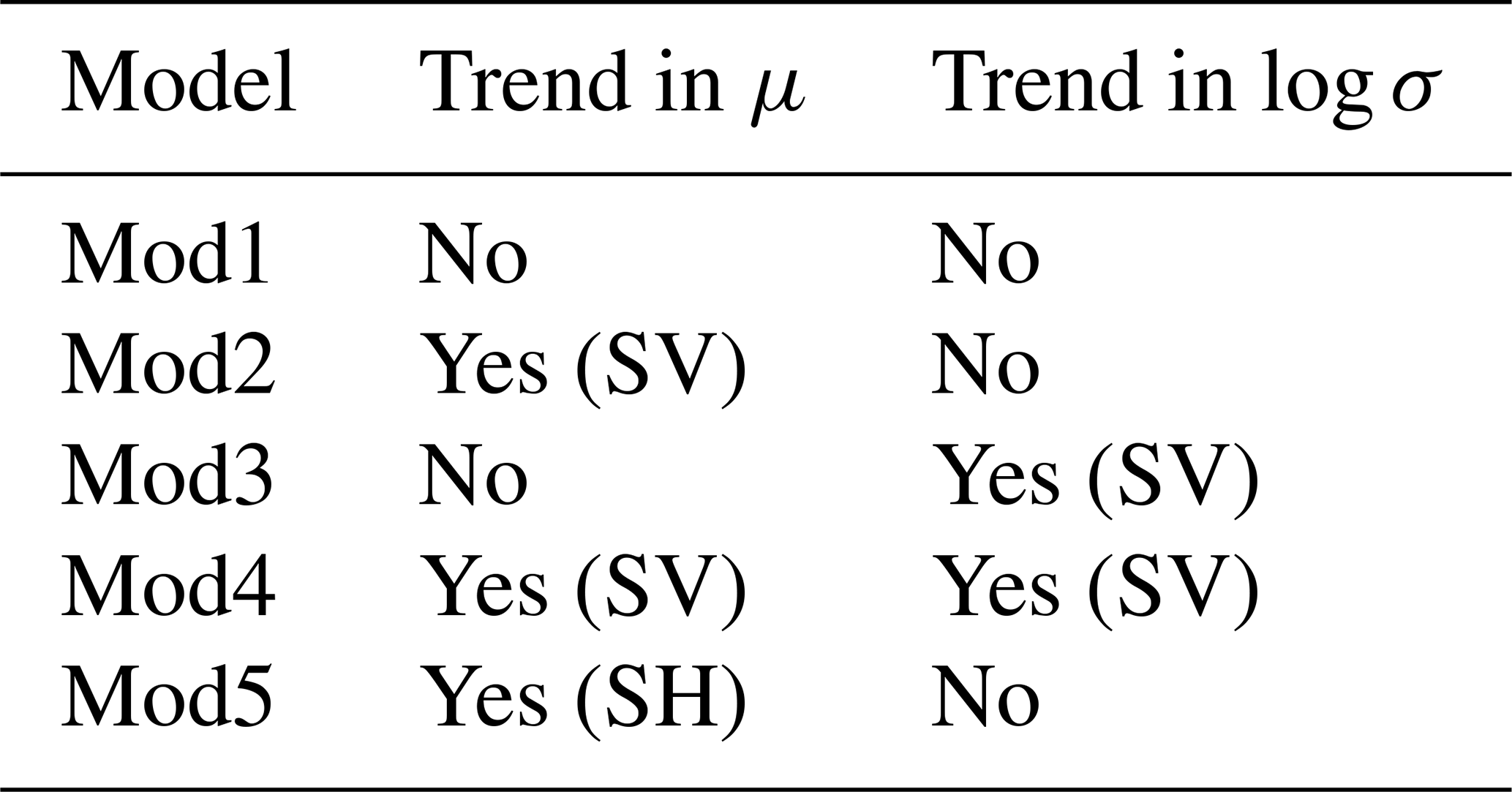
The model that has been described so far in this section contains only a single covariate in the GEV location parameter, and we have seen how the effect of this covariate on the annual maximum temperature can be modelled as smoothly varying over space by using the GMRF penalty. The value, xt, of the covariate in year t is taken to be the same at each grid box in year t, so that the covariate is spatially homogenous. We may also include spatially varying covariates in our model, and for this purpose we will include elevation (km) as a covariate in the GEV location parameter. From Fig. 3, it is clear that larger values of elevation tend to be associated with smaller values of the GEV location parameter. The framework of Wood et al. (2016) allows us to model covariates as having a generally smooth, rather than simply linear, effect on the location parameter. However, based on exploratory model fits, we find it adequate to specify elevation as having a linear effect on the GEV location term. We also consider models that have trends in the GEV scale parameter. In total, we consider five different models that differ from each other with regards to the inclusion of the covariate . For each model, it is assumed that , where, as before, Yit corresponds to the value of TXx in grid box i in year t. The differences between the models with regards to the inclusion of trends are summarized in Table 2. Consistent with most of the literature, we assume that the shape parameters vary only in space but not in time.
The most complex model is Mod4, which corresponds to the following formulas for the GEV parameters:
where , elevationi corresponds to the elevation (km) of grid box i minus the mean elevation across all grid boxes, and independent GMRF penalties are placed on and ξ. The fixed-effect β gives the change in the GEV location parameter for a 1 km increase in elevation. The trend in the scale parameter is modelled using the log link to ensure that the scale remains positive. Mod1, Mod2 and Mod3 are each special, simpler, cases of Mod4. In particular, Mod1 has μ1=0 and corresponding to the situation where there is no climate change signal detectable in TXx, whereas Mod2 and Mod3 correspond to the cases σ1=0 and μ1=0 respectively. Mod5 has only a trend in the GEV location parameter, but this is modelled as a fixed effect; i.e. the same trend is assumed at each geographic location, corresponding to and note that the trend μ1 does not depend on i.
Table 2Comparison of Mod1–Mod5 according to the inclusion of a trend in in the GEV location (μ) and log-scale (log σ) parameters and whether these trends are assumed to vary over space, i.e. are spatially varying (SV), or the same trend is assumed at each grid box, i.e. are spatially homogenous (SH). All the models include elevation (altitude) as a covariate.
To illustrate the effect and benefit of using the GMRF smoothing penalty, we compare, for region UKRI, the independent grid-box fits based on maximizing Eq. (4) separately for each i, using R package ismev, with joint maximization of the penalized log-likelihood (Eq. 6), with magnitude-adjusted likelihood, for the smooth model using evgam. The value of the constant k for the magnitude adjustment of the conditional independence likelihood was estimated to be 0.35.
Figure 4a and b show the fitted values of the GEV shape parameters, ξ, for the independent grid box and smooth model fits respectively. Although the broad spatial pattern of fitted shapes is similar in both cases, the fitted shapes for the smooth model encompass the more plausible range of −0.44 to −0.07 compared to the independent grid-box fits, which range from the extremely short tail of −0.71 to the heavy-tailed case of 0.16. The reduction in uncertainty that occurs by including neighbouring information in the model-fitting procedure is also illustrated in Fig. 4c. This shows the ratio in parameter uncertainty, as measured by the standard error, for the independent grid-box model fits relative to the smooth model. For the independent grid-box model fits, the standard errors were computed based on asymptotic normality of the maximum-likelihood estimators, and for the smooth model, standard errors were also computed based on asymptotic normality using the results of
Wood et al. (2016, Sect. 2). The mean ratio
is equal to approximately 3.7, which represents the average reduction in uncertainty achieved by including neighbouring information in the model fitting.
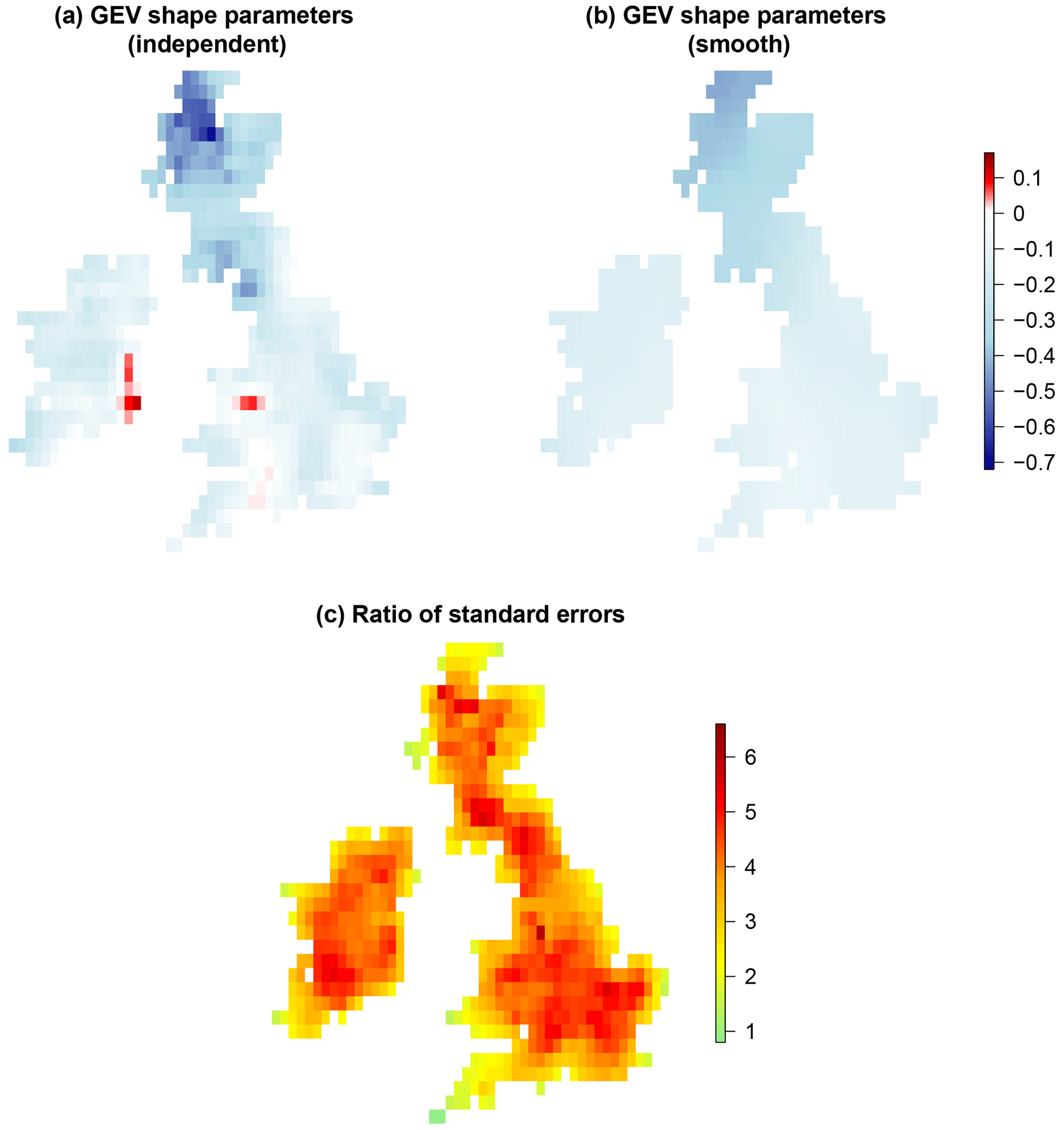
Figure 4Plots (a) and (b) show the fitted GEV shape parameters, ξ, for independent, i.e. separate, grid-box fits compared to a smooth model fit using the GMRF penalty. Plot (c) shows the ratio of the parameter uncertainty, as measured by the standard error, for the independent grid-box fits relative to the smooth model fit which uses information from neighbouring grid boxes.
3.3 Changes in return levels and risk ratios
In Sect. 3.1 we defined the return level with a return period to be the temperature that, in a stationary climate, is exceeded in a given year with probability p. In a non-stationary climate, this quantity will typically vary from year to year. For grid box i in year t, , we modify Eq. (3) and define yit(p) by
The quantity yit(p) may be interpreted as the return level with return period if the climate were stationary in the same state as in year t.
We consider for each grid box i the difference yi69(0.01)−yi1(0.01), which tells us the difference in the 100-year return levels in grid box i based on the 2018 and 1950 climates. We quantify the uncertainty in the return-level differences via Monte Carlo simulation. In particular, at each grid box, we sample 2000 values of μit,σit and ξit for t=1 and t=69 from their sampling distributions
and calculate the corresponding differences yi69(0.01)−yi1(0.01). We then calculate the 0.025 and 0.975 quantiles of these 2000 values to give us an approximate 95 % confidence interval for the return-level differences.
An example of how to perform these steps using the evgam package can be found in Sect. 4.3 of Youngman (2022).
Table 3Comparison of model scores, defined in Appendix A, by regions as defined in Table 1. The smallest, i.e. best, scores for each region are in bold. The scoring rules used are squared error (SE), Dawid–Sebastiani (DS), continuous ranked probability (CRP) and weighted continuous ranked probability (WCRP). AIC is the Akaike information criterion.
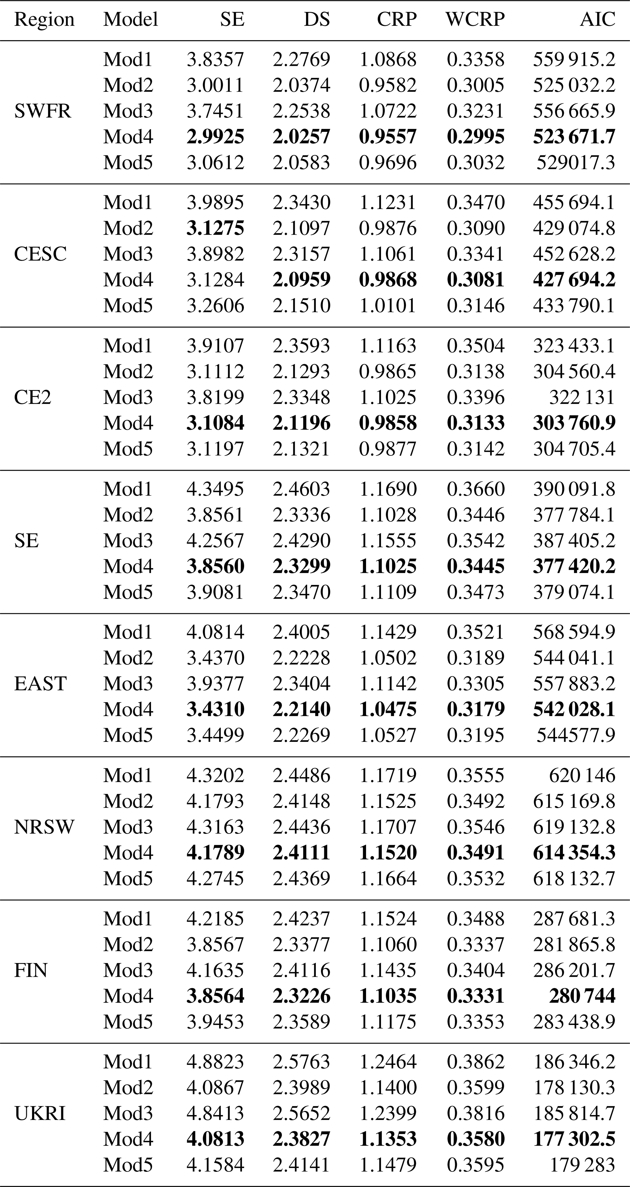
Table 4Approximate 95 % confidence intervals for the spatially averaged 100-year return-level differences (∘C), based on 2018 and 1950 climates (2018 return level subtract 1950 return level) and risk ratios for each region defined in Table 1. The results are based on Mod4, which includes a trend in the GEV location and log-scale parameters using the covariate log(). The endpoints of the intervals were calculated using Monte Carlo simulation. We simulated values of the GEV parameters from their sampling distributions at each grid box based on the 2018 and 1950 climates. We then calculated the return-level differences and risk ratios at each grid box and calculated the mean across the region. This procedure was repeated 2000 times. The and , with α=0.05, empirical quantiles of the 2000 estimated means give the left and right endpoints respectively of the intervals shown, where we have corrected for multiple comparisons using the Bonferroni correction. The more conservative (adjusted) intervals are based on the magnitude correction to the likelihood as in Ribatet et al. (2012).
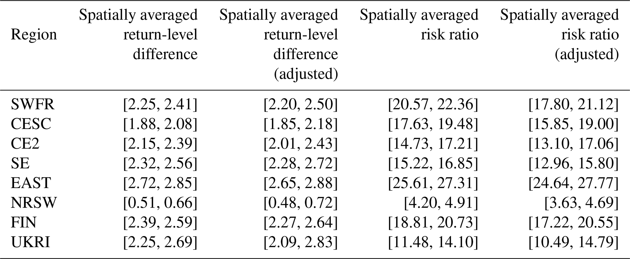
Table 5P values from a test of pair-wise exchangeability of CRP/WCRP scores for the two best models, Mod4 and Mod2, by region.
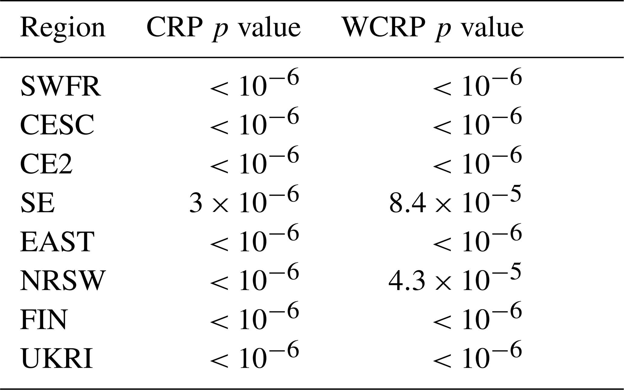
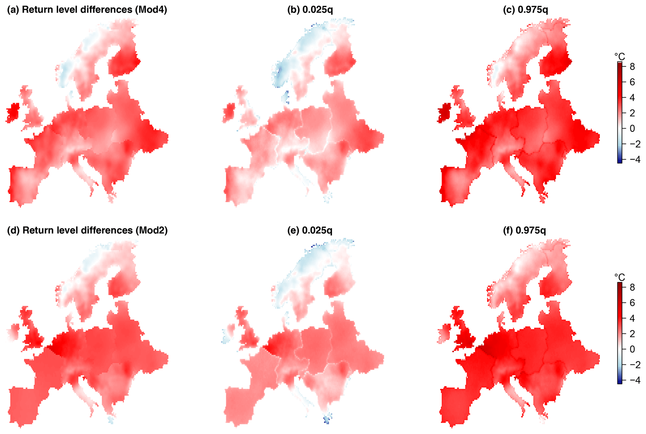
Figure 5The difference (∘C) in the 100-year return levels based on 2018 and 1950 climates (2018 return level subtract 1950 return level) and approximate 95 % confidence interval limits, calculated by Monte Carlo simulation as described in Sect. 3.3, for Mod4 (a, b, c) and Mod2 (d, e, f). Mod4 includes a trend in the GEV location and log-scale parameters using the covariate log(), whereas Mod2 only includes a trend in the GEV location parameter.
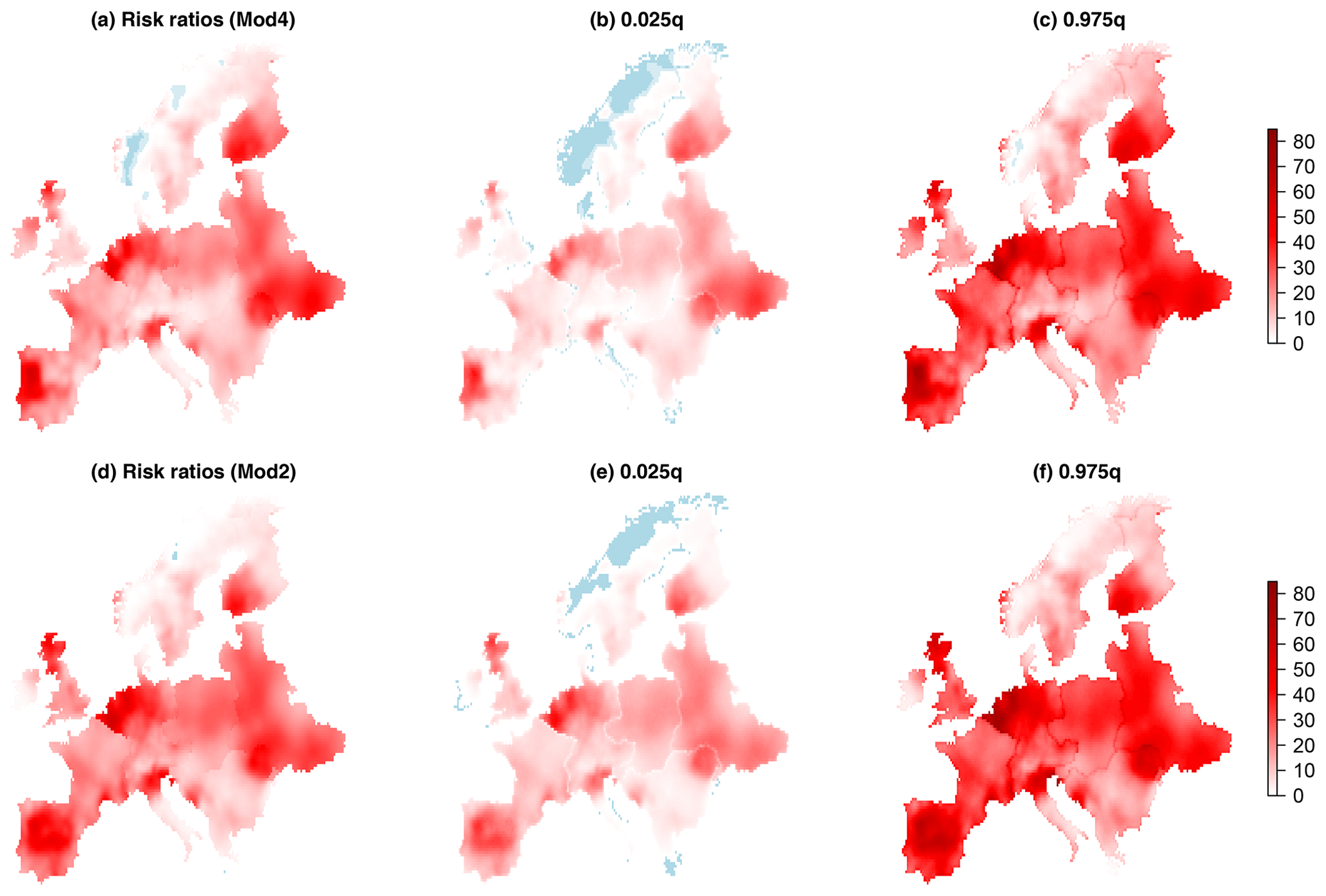
Figure 6Risk ratios and approximate 95 % confidence interval limits, calculated by Monte Carlo simulation as described in Sect. 3.3, for Mod4 (a, b, c) and Mod2 (d, e, f). Light blue corresponds to a risk ratio of less than one. Mod4 includes a trend in the GEV location and log-scale parameters using the covariate log(), whereas Mod2 only includes a trend in the GEV location parameter.
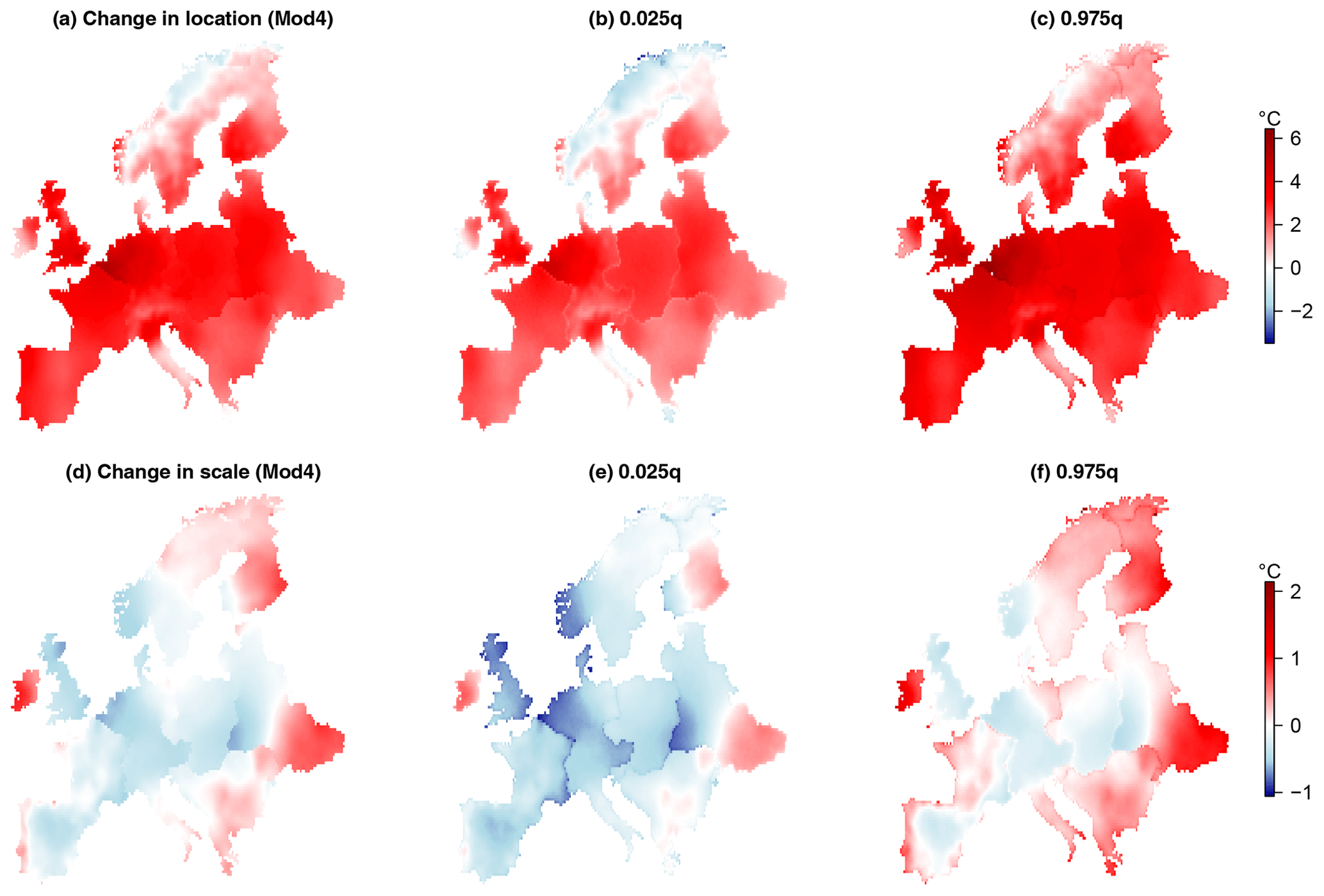
Figure 7Changes in the GEV location and scale parameters over the period 1950–2018 (2018 parameter values subtract 1950 values) and approximate 95 % confidence interval limits, calculated by Monte Carlo simulation as described in Sect. 3.3 for Mod4. Mod4 includes a trend in the GEV location and log-scale parameters using the covariate log().
Table 6Approximate 95 % confidence intervals for the spatially averaged changes in the GEV location and scale parameters (2018 parameter value subtract 1950 parameter value) for each region defined in Table 1. Calculations are based on Mod4, which has trends in GEV location and log-scale parameters using the covariate log(). The endpoints of the intervals are calculated by Monte Carlo simulation as described in the caption to Table 4. The more conservative (adjusted) intervals are based on the magnitude correction to the likelihood as in Ribatet et al. (2012).

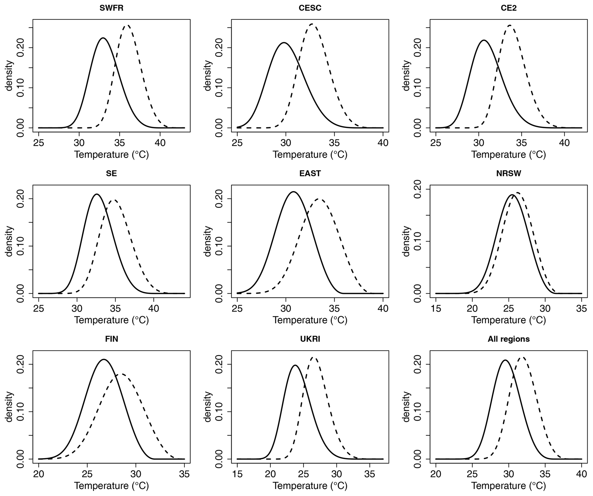
Figure 8Plots showing the distribution (density function) of TXx based on spatially averaged values of the fitted GEV parameters in 1950 (solid black curve) and 2018 (dashed curve) for each region defined in Table 1 and all regions together (bottom right plot). The GEV parameters in 1950 and 2018 are calculated using Mod4, which has trends in GEV location and log-scale parameters using the covariate log().
Another way that we quantify changes in the distribution of the annual maximum temperatures is via risk ratios (Titley et al., 2016). If Yit denotes a random variable with the same distribution as the annual maximum temperature in grid box i in year t, i.e. GEV with parameter vector , we consider the risk ratio
The value of the ratio (Eq. 8) then tells us, in grid box i, how many times more likely the 100-year return level based on the 1950 climate is to be exceeded in the 2018 climate. We quantify the uncertainty in the estimated risk ratio in the same way as the return-level difference, via simulation.
All the models were fitted using the R (R Core Team, 2021) package evgam (Youngman, 2022) on a Dell PowerEdge R430 computer running Scientific Linux 7 with four Intel Xeon E5-2680 v3 processors. As this is a shared departmental cluster, our access was restricted to 10 cores.
For a given fixed sub-region in Table 1, we assess the performance of each of the five models in Table 2 using several scoring rules (Gneiting and Raftery, 2007) in a 5-fold cross-validation (Stone, 1974; Hastie et al., 2009).
The scoring rules considered are the squared error (SE),
Dawid–Sebastiani (DS), continuous ranked probability (CRP) and the weighted continuous ranked probability (WCRP) scores. All the scoring rules we consider are negatively oriented, so that a smaller score indicates better performance.
Further information on the scoring rules and the cross-validation procedure can be found in Appendices A and B
respectively. For a given sub-region in Table 1 the cross-validation was performed in parallel using the R package parallel. The total compute time for the full cross-validation in all sub-regions was between 2 and 3 weeks.
A version of the Akaike information criterion (AIC) that is appropriate for the class of general smooth models we fit was developed in Wood et al. (2016), and we also report this value for each model. As with the scoring rules we consider, models with smaller AIC values are preferred.
Within the main text and figures, all reported confidence intervals are based on the magnitude-adjusted likelihood of Ribatet et al. (2012) as described in Sect. 3.2.
Table 3 shows the mean scores of each model by region from 5-fold cross-validation. These scores are based on the conditional independence likelihood model fits using Eq. (6). The corresponding model scores (not shown) when performing the magnitude adjustment to the likelihood are very similar, leading to the same conclusions. For all regions, Mod4, which includes a spatially varying trend in both the GEV location and log-scale parameters, is the best-performing model, closely followed by Mod2, which only contains the spatially varying trend in the GEV location parameter. Mod5, which has a fixed effect of the covariate in the location parameter, i.e. a constant trend at all grid boxes in a given sub-region, is generally the next best-performing model. Mod1, which has all of the GEV parameters fixed in time, is the worst-performing model in all regions according to all the scores, followed by Mod3, which has only a spatially varying trend in the GEV log-scale parameter.
Table 5 shows the p values, by region, of the hypothesis test that the CRP scores shown in Table 3 for Mod4 and Mod2 (the two best-performing models) are pair-wise exchangeable. The testing procedure is described in Appendix B. Failure to reject the null hypothesis would, informally, mean that the performances of Mod4 and Mod2 are statistically indistinguishable. In all regions, the null hypothesis of pair-wise exchangeability is rejected at the 0.05 and 0.01 levels of significance after adjusting the raw p values in Table 5 using the Bonferroni correction for multiple comparisons, giving evidence in favour of the better-performing Mod4. We also perform the same test for the WCRP scores of Mod4 and Mod2. For all regions the null hypothesis of pair-wise exchangeability of WCRP scores is rejected at the 0.05 and 0.01 level of significance, giving evidence in favour of Mod4. Thus, we find strong evidence in favour of both changes in location and scale of the distributions of TXx since 1950.
Figure 5 shows the difference in 100-year return levels based on the 2018 and 1950 climates, for both Mod4 and Mod2, along with approximate 95 % confidence intervals, calculated using Monte Carlo simulation, as described in Sect. 3.3. The corresponding risk ratio plots are shown in Fig. 6. Mod2, which only has a trend in the GEV location parameter, tends to find slightly larger increases in the 100-year return levels based on the 2018 climate compared to 1950, but the spatial pattern broadly agrees with that produced by Mod4, and similar comments apply for the risk ratios. All the regions show, on average, significant increases in return levels and risk ratios greater than one, as shown in Table 4. Region NRSW, comprising Norway and Sweden, stands out as having relatively moderate changes compared to the other regions, with the mean increase over the region in the 100-year return level being around 0.6 ∘C. There are several locations within this region where negative changes are detected, although upon inspecting the approximate 95 % confidence intervals in Figs. 5 and 6, most of these changes do not appear to be significant. Even in this region of relatively modest changes, the 100-year return level based on the 1950 climate is estimated to be, on average, approximately 4 times more likely to be exceeded in the 2018 climate. The region EAST comprising eastern European countries shows the most dramatic increases, with a mean 100-year return-level difference of around 2.8 ∘C and a mean risk ratio in excess of 26. Averaging over the entire spatial domain, we find that, under Mod4 (change in location and scale), the mean difference between the 100-year return levels based on the 2018 and 1950 climates is 2.08 ∘C, with a 95 % confidence interval of [2.03,2.12]. For Mod2 (change in location only), the mean difference is 2.29 ∘C, with a 95 % confidence interval of Similarly, under Mod4, the mean risk ratio over the entire spatial domain is 16.12, with a 95 % confidence interval of [15.74,16.53], so that on average a 100-year return level in the 1950 climate corresponds approximately to a 6-year return level in the 2018 climate. For Mod2, the mean risk ratio is increased to 18.00, with a 95 % confidence interval of [17.65,18.34].
Changes in the GEV location and scale parameters over the period 1950 to 2018 calculated using Mod4 are shown in Fig. 7. Approximately 96 % of the grid boxes show an increase in the location parameter over the study period, and after calculating approximate 95 % confidence intervals for each change in location, 88 % of these have a lower limit greater than zero. We cannot however conclude that warming is detected in TXx in 88 % of grid boxes as we make no attempt to correct for multiple comparisons. The changes in the GEV scale show rather more variability, with 37 % positive and 63 % negative fitted values. After calculating approximate 95 % confidence intervals for the scale changes, approximately 50 % of these slopes contain 0. The spatially averaged changes in the GEV location and scale parameters for each sub-region in Table 1 are shown in Table 6, and the spatially averaged distributions of TXx in 1950 and 2018 are shown for each sub-region in Fig. 8. All the regions show, on average, significant increases in the GEV location parameter, indicating a tendency for TXx to shift towards hotter temperatures. There is a mixture of both increases and decreases in the spatially averaged GEV scale parameter differences corresponding to increasing and decreasing variabilities of TXx respectively. The regions with an average increase in the GEV scale parameter occur in the east and in Ireland. We find that, under Mod4, a 95 % confidence interval for the spatially averaged change in the GEV location parameter over all regions is [2.28,2.32], whereas the corresponding interval for the change in scale is . Thus, although there is a strong signal for shifts of the TXx distributions in all regions towards hotter temperatures, as indicated by the positive changes in the GEV location, the mixtures of increases and decreases in the GEV scale parameter approximately cancel each other out when spatially averaged across our study region. The changes in the GEV location parameter for Mod2 are the same as the return-level differences shown in the bottom row of Fig. 5.
In the same notation as Sect. 3.2, for Mod4, a test of the null hypothesis μ1=0, i.e. all location slopes are zero, using the asymptotic distributional results of Wood et al. (2016), has for each region a p value of less than , giving strong evidence against the null hypothesis. The same result is found for the location slopes from Mod2 and log-scale slopes for Mod4. Together with the results in Table 3, the hypothesis of no temporal variation in the GEV parameters is strongly rejected in all regions, supporting robust detection of changing TXx distributions over time.
We have considered the problem of detecting and quantifying large-scale changes in the distributions of the annual maximum daily maximum temperature (TXx) in a large subset of Europe during the years 1950–2018. Our approach was to divide the full domain into eight sub-regions over which several statistical models were fitted. In each of the models considered, TXx at each grid box was modelled using a generalized extreme-value (GEV) distribution with the GEV location and scale parameters allowed to vary in time using atmospheric CO2 as a covariate. We modelled the GEV parameters as varying smoothly over space, where the appropriate degree of smoothness was determined objectively using the methods of Wood et al. (2016). Changes were detected most strongly in the GEV location parameter, with the distributions of TXx shifting towards hotter temperatures at most grid boxes. Although the best-performing model in all regions has both the GEV location and scale parameters changing in time, the signal for changes in the scale parameters is noisier than that for the location parameters, with some regions showing a tendency to increases in scale and others a decrease. The regions that show a tendency to an increase in scale, corresponding to an increase in the variability in TXx, are in eastern Europe and Ireland. The second-best-performing model in all regions has only the GEV location parameter changing in time. Regardless of whether our best or second-best models were used, our main findings regarding changes in return levels based on the 2018 and 1950 climates and risk ratios broadly agree. Using our best-performing model and averaging across our entire spatial domain, the 100-year return level of TXx based on the 2018 climate is approximately 2 ∘C hotter than that based on the 1950 climate. Also averaging across our spatial domain, the 100-year return level of TXx based on the 1950 climate corresponds approximately to a 6-year return level in the 2018 climate. Our findings are most robust in central Europe, where the underlying network of weather stations used to construct the gridded data set has the highest density. Finally, although we made an effort to mitigate against well-known deficiencies of gridded station data, namely inhomogeneities and low station density regions, the data we used will nonetheless be imperfect. It would therefore be of great interest to see how well our findings may be replicated using different data sources in future studies.
We use several scoring rules that evaluate the performance of models based on their ability to predict unseen data, i.e. data that were held out from the model-fitting procedure. A scoring rule is a function, S, that assigns a real number value S(F,y) to the pair (F,y), where F is a distribution function and y is an observed value. In our case F will be the cumulative distribution function of a fitted GEV distribution and y will be some observation, held out from the model-fitting procedure, that under our model is assumed to be drawn from F. Intuitively, the value of S(F,y) can be thought of as measuring the extent to which the distribution F and observation y are compatible. All of the scoring rules that we consider are negatively oriented, so that smaller scores correspond to better predictions.
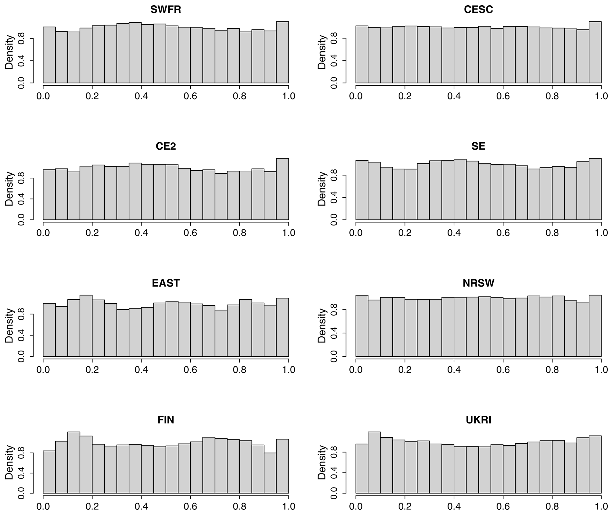
Figure A1Histograms of probability integral transform (PIT) values by region for Mod4. If the model is correct, the PIT values are uniformly distributed.
A negatively oriented scoring rule S is called proper (Gneiting and Raftery, 2007) if
where 𝔼 denotes expectation; i.e. on average, the true distribution G will not give a worse score than any other distribution F, so that forecasters are incentivized to report the truth. All the scores that we consider are proper. If equality in Eq. (A1) holds only if F=G, then S is called strictly proper.
One of the simplest and most common scoring rules is the squared error score SSE defined by
where μF is the expected value of a random variable with distribution F. The squared error score gives higher penalties the further an observation is from the mean of the distribution but may be regarded as rather simplistic in that the distribution F is represented in the score only through its mean μF. When the variance of F is large, we may wish to give a smaller penalty to observations y that are far from the mean μF. One score that does this is the Dawid–Sebastiani score, SDS, defined by
where is the variance of F.
Another commonly used scoring rule is the continuous ranked probability score (CRPS) defined by
Unlike the squared error and Dawid–Sebastiani scores, the CRPS takes into account the full distribution F and compares it with the empirical distribution based on the single observation y. A closed-form expression for the CRPS when F is the distribution function of a GEV random variable is given in Friederichs and Thorarinsdottir (2012) and implemented in the R package scoringRules (Jordan et al., 2019).
For an extreme-value analysis, it may be desirable to consider a scoring rule that gives a higher penalty for poor prediction in the tails of the distribution. One way to do this is to use a weighted version of the CRPS (Gneiting and Ranjan, 2011). First, we note that an alternative representation of the CRPS in terms of quantiles is
The equality of Eqs. (A4) and (A5) is shown in Laio and Tamea (2006). The weighted continuous ranked probability score (WCRPS) is obtained from Eq. (A5) by adding an extra factor, w(p), to the integrand, which determines the weight given to the pth quantile giving
In our application we use the weighting function w(p)=p2. As the integral Eq. (A6) does not have a closed-form solution when F is the distribution function of a GEV random variable, we approximate it with the summation
for large N and a partition of the interval [0,1]. In our case we take the evenly spaced partition with N=1000 and .
We use each of the scoring rules described above as part of a cross-validation scheme to evaluate a model's performance. This is described in Appendix B.
For each of the regions in Table 1, we evaluate the performance of each of the models in Table 2 using 5-fold cross-validation. Specifically, for a fixed region, we randomly assign each observation of the region to one of five subsets, or splits, of approximately equal size. The same splits are used in each model evaluation. Suppose there are Nj observations in split , which we denote by . We fix one of the splits, k say, , to be used as test data and fit the model of interest to the data from the remaining four splits. For each observation , from the test data, we evaluate for each of the scores defined in Appendix A, where is the GEV distribution function that, under the fitted model, is assumed to be drawn from. This procedure is carried out for each , so that each split gets used as test data. The mean score, , where is the total number of observations in the region, gives an overall measure of model performance according to score S. For the scores defined in Appendix A, which are all negatively oriented, models with lower mean scores are preferred.
Suppose that in the cross-validation procedure described above, model B produces a lower mean score than another model, A. If the observed difference in the mean scores is very small, we may wish to test whether this really provides evidence that model B is better than model A. Suppose that, for each model, we have the N scores and , , where and are the distribution functions that, under models A and B respectively, observation yi is assumed to be drawn from. We will construct a test for the null hypothesis that the scores and are pair-wise exchangeable for . Two random variables X1 and X2 are said to be exchangeable if In particular, this implies that X1 and X2 are identically distributed. If the scores and are pair-wise exchangeable, then the score would be equally likely to have been produced by model B, and similarly, is equally likely to have been produced by model A. Thus, for the observed score difference , we would have been equally likely to have observed under the null hypothesis. This motivates the following randomized test procedure defined in Algorithm B1 below.
Algorithm B1Hypothesis testing procedure for testing pair-wise exchangeability of model scores.
The value of p computed in Algorithm B1 is an unbiased estimate of the one-sided p value for the test with null hypothesis that the scores and are pair-wise exchangeable, . The value of the observed test statistic Tobs is strictly positive since it is assumed that model B has the lower observed mean score. Small values of p give evidence against the null hypothesis in favour of model B. In our applications of Algorithm B1, we take J=106.
In this Appendix we perform some visual checks for Mod4 to see whether this model provides a reasonable fit to the data and is not merely the best of a bad bunch of models. As it is not feasible to provide plots for every grid box, we consider the performance as a whole over the sub-regions as defined in Table 1.
One simple way to check for any systematic discrepancies between a fitted model and the observed data is to use the probability integral transform (PIT). The PIT states that, if Y is a random variable with continuous distribution function F, then the random variable F(Y) is uniformly distributed between 0 and 1. Suppose that, given a sample of size n with observed response variables, yi, , a statistical model fits distribution function Fi to yi. Then, if the model is correct, the values Fi(yi), are a sample of size n from a uniform distribution on [0,1]. The plausibility of this may be checked visually, e.g. by plotting a histogram of the n PIT values Fi(yi), . A U-shaped histogram would indicate that the fitted model is underdispersive; i.e. it does not adequately account for the variability in the data, whereas a histogram that is too peaked in the middle indicates that the model is overdispersive. Histograms of the PIT values, by region, are shown for Mod4 in Fig. A1 and do not show any serious cause for concern.
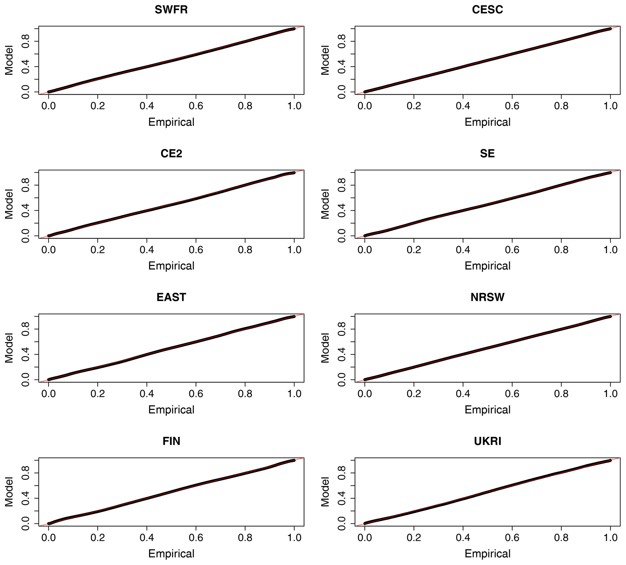
Another standard method for checking a non-stationary extreme-value model fit is via probability or quantile plots (Coles, 2001, Sect. 6.2.3). Both of these plots are based on the fact that if Yit is a GEV random variable with parameters , then the variable Zit defined by
has a standard Gumbel distribution with distribution function . If we fix a specific region in Table 1 and suppose that, as in Sect. 3.1, in grid box i we have observed annual maxima, , then, from a given fitted model, we may obtain the values by applying the transformation Eq. (C1). If there are N grid boxes in the region in total, then we may apply this transformation to all grid boxes and obtain transformed z values. If the model is correct, then the ordered values where z(k)≤z(l) when k≤l would be a sample from a standard Gumbel distribution. The probability plot tests the plausibility of this by comparing empirical and fitted-model probabilities and plots the pairs

The quantile plot compares fitted-model and empirical quantiles and plots the pairs
The further these plots deviate from a diagonal line, the greater the discrepancy between the fitted model and the observations. Probability and quantile plots are shown by region in Figs. B1 and C1. The probability plots stay very close to the diagonal line, indicating a good quality of fit for each sub-region. The quantile plots show, to a varying extent in each region, some discrepancy in the upper tail. For the sake of reference, the values 5, 6, 7 and 8 correspond to the 0.9933, 0.9975, 0.9991 and 0.9997 theoretical quantiles of the standard Gumbel distribution respectively. Thus we can see that Mod4 gives a good fit in all regions at least up to the 0.9933 regional quantile and in several regions beyond this but fails to explain approximately the largest 0.05 % of observations in each region. Given the very large quantities of data in each region, this is of no great surprise or concern.
Finally, we inspect the spatial distribution of the Pearson residuals obtained from a model fit. For grid box i we obtain the ni residuals defined by
where and denote the model-fitted expected value and standard deviation respectively. When the fitted distribution is GEV with parameter vector , then these expressions become
and
where γ≈0.5772 is Euler's constant and If the fitted model were correct, then the Pearson residuals are realizations of a random variable with mean 0 and standard deviation 1. The mean and standard deviation of the Pearson residuals for each grid box for both Mod4 and Mod2 are shown in Fig. D1. The spatial distributions look similar for both models and do not display any worryingly large deviations from the zero mean, unit standard deviation assumption.
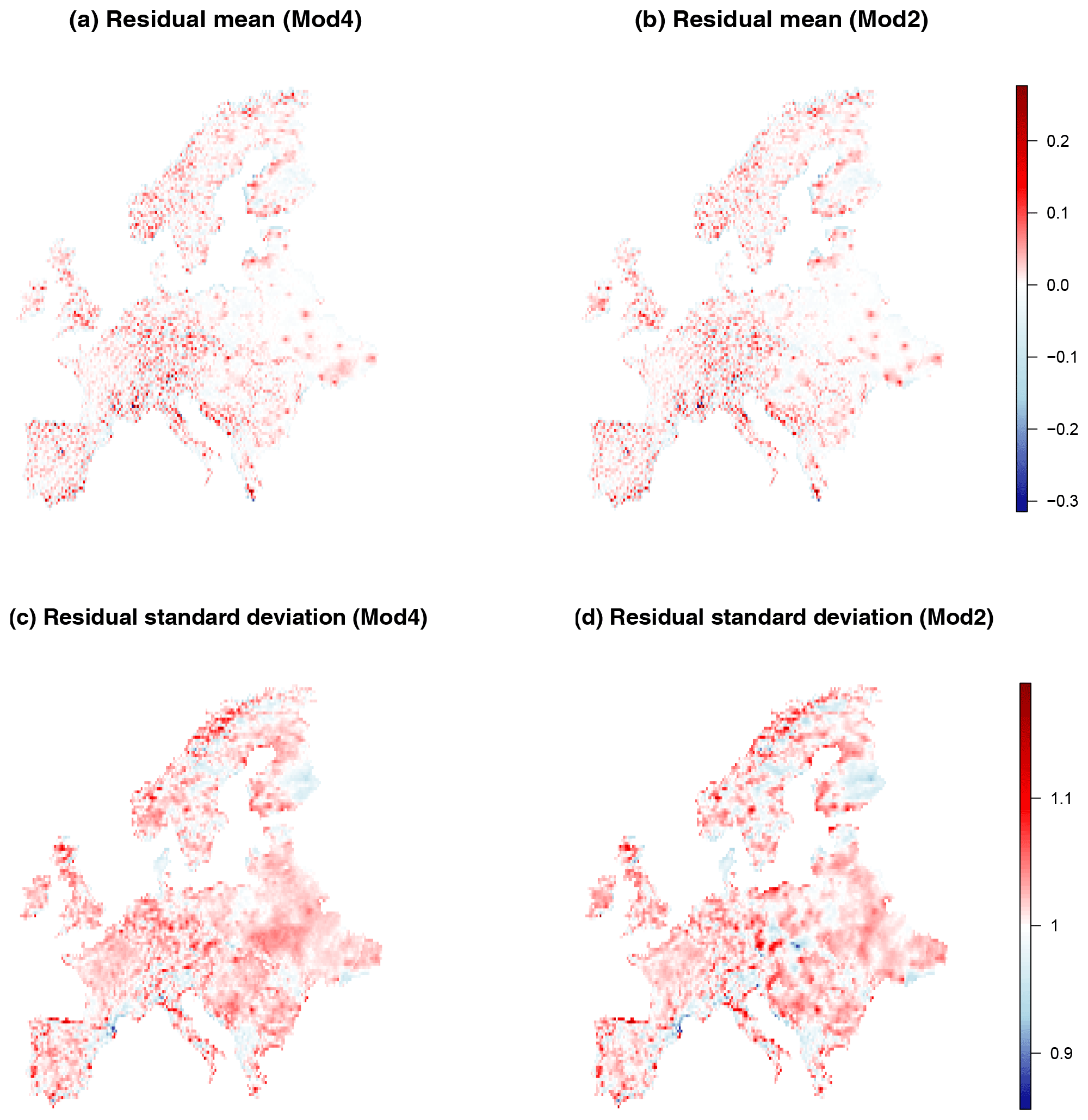
Figure D1Mean values (a, b) and standard deviations (c, d) of Pearson residuals for Mod4 and Mod2.
The data analysed in this paper are publicly available from https://www.ecad.eu/download/ensembles/downloadversion19.0eHOM.php (European Climate Assessment & Dataset project with Horizon 2020 EUSTACE project, 2023). Regional R data frames for each of the regions defined in Table 1 and R scripts for fitting models and performing cross-validation and diagnostics are available from https://doi.org/10.6084/m9.figshare.21257217.v1 (Auld et al., 2023).
All the authors are responsible for the conceptualization of the research. GA carried out the formal analysis, developed the methodology and wrote the original draft. All the authors discussed the results and helped with review and editing of the final draft. Both IP and GCH acted as supervisors to GA.
The contact author has declared that none of the authors has any competing interests.
Publisher’s note: Copernicus Publications remains neutral with regard to jurisdictional claims in published maps and institutional affiliations.
We are grateful to Ben Youngman for helpful advice regarding use of the evgam package and to two anonymous reviewers for helpful comments on an earlier draft of the manuscript.
Graeme Auld is supported financially by the Ratchadapisek Somphot Fund for Postdoctoral Fellowship, Chulalongkorn University, and was supported during his PhD, when much of this research took place, by the EPSRC (grant no. 1935526). Gabriele C. Hegerl has been supported by NERC grant EMERGENCE (grant no. NE/S004661/1).
This paper was edited by Seung-Ki Min and reviewed by two anonymous referees.
Allen, M., Dube, O., Solecki, W., Aragón-Durand, F., Cramer, W., Humphreys, S., Kainuma, M., Kala, J., Mahowald, N., Mulugetta, Y., Perez, R., Wairiu, M., and Zickfeld, K.: Framing and Context, in: Global Warming of 1.5°C. An IPCC Special Report on the impacts of global warming of 1.5°C above pre-industrial levels and related global greenhouse gas emission pathways, in the context of strengthening the global response to the threat of climate change, sustainable development, and efforts to eradicate poverty, edited by: Masson-Delmotte, V., Zhai, P., Pörtner, H.-O., Roberts, D., Skea, J., Shukla, P. R., Pirani, A., Moufouma-Okia, W., Péan, C., Pidcock, R., Connors, S., Matthews, J. B. R., Chen, Y., Zhou, X., Gomis, M. I., Lonnoy, E., Maycock, T., Tignor, M., and Waterfield, T., World Meteorological Organization, Geneva, Switzerland, https://www.ipcc.ch/sr15/chapter/chapter-1/ (last access: 16 May 2023), https://doi.org/10.1017/9781009157940.003, 2018. a
Andrade, C., Leite, S. M., and Santos, J. A.: Temperature extremes in Europe: overview of their driving atmospheric patterns, Nat. Hazards Earth Syst. Sci., 12, 1671–1691, https://doi.org/10.5194/nhess-12-1671-2012, 2012. a
Auld, G., Papastathopoulos, I., and Hegerl, G.: DataAndCode.zip, figshare [data set], https://doi.org/10.6084/m9.figshare.21257217.v1, 2023. a
Banerjee, S., Carlin, B., and Gelfand, A.: Hierarchical Modeling and Analysis for Spatial Data, Monographs on Statistical and Applied Probability, Chapman & Hall/CRC, New York, https://doi.org/10.1201/b17115, 2004. a
Basu, R. and Samet, J.: Relation between elevated ambient temperature and mortality: a review of the epidemiologic evidence, Epidemiol. Rev., 24, 190–202, https://doi.org/10.1093/epirev/mxf007, 2002. a
Brunsdon, C., Fotheringham, S., and Charlton, M.: Geographically weighted regression-modelling spatial non-stationarity, J. Roy. Stat. Soc. Ser. D, 47, 431–443, https://doi.org/10.1111/1467-9884.00145, 1998. a
Bücher, A. and Segers, J.: On the maximum likelihood estimator for the Generalized Extreme-Value distribution, Extremes, 20, 839–872, https://doi.org/10.1007/s10687-017-0292-6, 2017. a
Chandler, R. E. and Bate, S.: Inference for clustered data using the independence loglikelihood, Biometrika, 94, 167–183, https://doi.org/10.1093/biomet/asm015, 2007. a
Charney, J., Arakawa, A., Baker, D., Bolin, Dickinson, B. R., Goody, R., Leith, C., Stommel, H., and Wunsch, C.: Carbon Dioxide and Climate: A Scientific Assessment, The National Academies Press, Washington, DC, https://doi.org/10.17226/12181, 1979. a
Chavez-Demoulin, V. and Davison, A. C.: Generalized additive modelling of sample extremes, J. Roy. Stat. Soc. Ser. C, 54, 207–222, https://doi.org/10.1111/j.1467-9876.2005.00479.x, 2005. a
Chen, S.-Y., Feng, Z., and Yi, X.: A general introduction to adjustment for multiple comparisons, J. Thorac. Dis., 9, 1725–1729, https://doi.org/10.21037/jtd.2017.05.34, 2017. a
Coles, S. and Dixon, M.: Likelihood-based inference for extreme value models, Extremes, 2, 5–23, https://doi.org/10.1023/A:1009905222644, 1999. a
Coles, S. G.: An Introduction to Statistical Modeling of Extreme Values, Springer-Verlag, London, https://doi.org/10.1007/978-1-4471-3675-0, 2001. a, b
Cornes, R., Schrier, G., Van den Besselaar, E., and Jones, P.: An ensemble version of the E-OBS temperature and precipitation data sets, J. Geophys. Res.-Atmos., 123, 9391–9409, https://doi.org/10.1029/2017JD028200, 2018. a, b
Davison, A. C. and Smith, R. L.: Models for exceedances over high thresholds, J. Roy. Stat. Soc. Ser. B, 52, 393–442, https://doi.org/10.1111/j.2517-6161.1990.tb01796.x, 1990. a
de Bono, A., Giuliani, G., Kluser, S., and Peduzzi, P.: Impacts of summer 2003 heat wave in Europe, UNEP/DEWA/GRID Eur. Environ. Alert Bull., 2, 1–4, https://www.unisdr.org/files/1145_ewheatwave.en.pdf (last access: 16 May 2023), 2004. a
Doblas-Reyes, F., Sörensson, A., Almazroui, M., Dosio, A., Gutowski, W., Haarsma, R., Hamdi, R., Hewitson, B., Kwon, W.-T., Lamptey, B., Maraun, D., Stephenson, T., Takayabu, I., Terray, L., Turner, A., and Zuo, Z.: Linking Global to Regional Climate Change, in: Climate Change 2021: The Physical Science Basis, Contribution of Working Group I to the Sixth Assessment Report of the Intergovernmental Panel on Climate Change, edited by: Masson-Delmotte, V., Zhai, P., Pirani, A., Connors, S. L., Péan, C., Berger, S., Caud, N., Chen, Y., Goldfarb, L., Gomis, M. I., Huang, M., Leitzell, K., Lonnoy, E., Matthews, J. B. R., Maycock, T. K., Waterfield, T. K., Yelekçi, O., Yu, R., and Zhou, B., Cambridge University Press, Cambridge, United Kingdom and New York, NY, USA, https://www.ipcc.ch/report/ar6/wg1/chapter/chapter-10/ (last access: 16 May 2023), 2021. a
Donat, M. and Alexander, L.: The shifting probability distribution of global daytime and night‐time temperatures, Geophys. Res. Lett., 39, L14707, https://doi.org/10.1029/2012GL052459, 2012. a
Dunn, R. J. H., Alexander, L. V., Donat, M. G., Zhang, X., Bador, M., Herold, N., Lippmann, T., Allan, R., Aguilar, E., Barry, A. A., Brunet, M., Caesar, J., Chagnaud, G., Cheng, V., Cinco, T., Durre, I., de Guzman, R., Htay, T. M., Wan Ibadullah, W. M., Bin Ibrahim, M. K. I., Khoshkam, M., Kruger, A., Kubota, H., Leng, T. W., Lim, G., Li-Sha, L., Marengo, J., Mbatha, S., McGree, S., Menne, M., de los Milagros Skansi, M., Ngwenya, S., Nkrumah, F., Oonariya, C., Pabon-Caicedo, J. D., Panthou, G., Pham, C., Rahimzadeh, F., Ramos, A., Salgado, E., Salinger, J., Sané, Y., Sopaheluwakan, A., Srivastava, A., Sun, Y., Timbal, B., Trachow, N., Trewin, B., van der Schrier, G., Vazquez-Aguirre, J., Vasquez, R., Villarroel, C., Vincent, L., Vischel, T., Vose, R., and Bin Hj Yussof, M. N.: Development of an Updated Global Land In Situ-Based Data Set of Temperature and Precipitation Extremes: HadEX3, J. Geophys. Res.-Atmos., 125, e2019JD032263, doi10.1029/2019JD032263, 2020. a
European Climate Assessment & Dataset project with Horizon 2020 EUSTACE project: E-OBS v19.0HOM gridded dataset, https://www.ecad.eu/download/ensembles/downloadversion19.0eHOM.php, last access: 16 May 2023. a
Eyring, V., Bony, S., Meehl, G. A., Senior, C. A., Stevens, B., Stouffer, R. J., and Taylor, K. E.: Overview of the Coupled Model Intercomparison Project Phase 6 (CMIP6) experimental design and organization, Geosci. Model Dev., 9, 1937–1958, https://doi.org/10.5194/gmd-9-1937-2016, 2016. a
Farcomeni, A.: A review of modern multiple hypothesis testing, with particular attention to the false discovery proportion, Stat. Meth. Med. Res., 17, 347–388, https://doi.org/10.1177/0962280206079046, 2008. a
Fischer, E. and Schär, C.: Consistent geographical patterns of changes in high-impact European heatwaves, Nat. Geosci., 3, 398–403, https://doi.org/10.1038/ngeo866, 2010. a
Friederichs, P. and Thorarinsdottir, T. L.: Forecast verification for extreme value distributions with an application to probabilistic peak wind prediction, Environmetrics, 23, 579–594, https://doi.org/10.1002/env.2176, 2012. a
Gilleland, E. and Katz, R. W.: extRemes 2.0: An Extreme Value Analysis Package in R, J. Stat. Softw., 72, 1–39, https://doi.org/10.18637/jss.v072.i08, 2016. a
Gneiting, T. and Raftery, A. E.: Strictly proper scoring rules, prediction, and estimation, J. Am. Stat. Assoc., 102, 359–378, https://doi.org/10.1198/016214506000001437, 2007. a, b
Gneiting, T. and Ranjan, R.: Comparing density forecasts using threshold-and quantile-weighted scoring rules, J. Bus. Econ. Stat., 29, 411–422, https://doi.org/10.1198/jbes.2010.08110, 2011. a
Hastie, T. and Tibshirani, R.: Varying-coefficient models, J. Roy. Stat. Soc. Ser. B, 55, 757–779, https://doi.org/10.1111/j.2517-6161.1993.tb01939.x, 1993. a
Hastie, T., Tibshirani, R., and Friedman, J.: The Elements of Statistical Learning: Data Mining, Inference and Prediction, Springer Series in Statistics, Springer, New York, 2nd Edn., https://doi.org/10.1007/978-0-387-84858-7, 2009. a
Haug, O., Thorarinsdottir, T. L., Sørbye, S. H., and Franzke, C. L. E.: Spatial trend analysis of gridded temperature data at varying spatial scales, Adv. Stat. Clim. Meteorol. Oceanogr., 6, 1–12, https://doi.org/10.5194/ascmo-6-1-2020, 2020. a, b
Heffernan, J. E. and Stephenson, A.: ismev: An Introduction to Statistical Modeling of Extreme Values, https://cran.r-project.org/web/packages/ismev/ismev.pdf (last access: 16 May 2023), 2018. a
Hersbach, H., Bell, B., Berrisford, P., Hirahara, S., Horányi, A., Muñoz-Sabater, J., Nicolas, J., Peubey, C., Radu, R., Schepers, D., Simmons, A., Soci, C., Abdalla, S., Abellan, X., Balsamo, G., Bechtold, P., Biavati, G., Bidlot, J., Bonavita, M., De Chiara, G., Dahlgren, P., Dee, D., Diamantakis, M., Dragani, R., Flemming, J., Forbes, R., Fuentes, M., Geer, A., Haimberger, L., Healy, S., Hogan, R. J., Hólm, E., Janisková, M., Keeley, S., Laloyaux, P., Lopez, P., Lupu, C., Radnoti, G., de Rosnay, P., Rozum, I., Vamborg, F., Villaume, S., and Thépaut, J.-N.: The ERA5 global reanalysis, Q. J. Roy. Meteor. Soc., 146, 1999–2049, doi10.1002/qj.3803, 2020. a
Hoegh-Guldberg, O., Jacob, D., Taylor, M., Bindi, M., Brown, S., Camilloni, I., Diedhiou, A., Djalante, R., Ebi, K., Engelbrecht, F., Guiot, J., Hijioka, Y., Mehrotra, S., Payne, A., Seneviratne, S., Thomas, A., Warren, R., and Zhou, G.: Impacts of 1.5°C of Global Warming on Natural and Human Systems, in: Global Warming of 1.5°C. An IPCC Special Report on the impacts of global warming of 1.5°C above pre-industrial levels and related global greenhouse gas emission pathways, in the context of strengthening the global response to the threat of climate change, sustainable development, and efforts to eradicate poverty, edited by: Masson-Delmotte, V., Zhai, P., Pörtner, H.-O., Roberts, D., Skea, J., Shukla, P. R., Pirani, A., Moufouma-Okia, W., Péan, C., Pidcock, R., Connors, S., Matthews, J. B. R., Chen, Y., Zhou, X., Gomis, M. I., Lonnoy, E., Maycock, T., Tignor, M., and Waterfield, T., World Meteorological Organization, Geneva, Switzerland, https://www.ipcc.ch/sr15/chapter/chapter-3/ (last access: 16 May 2023), 2018. a
Hofstra, N., Haylock, M., New, M., and Jones, P.: Testing E-OBS European high-resolution gridded data set of daily precipitation and surface temperature, J. Geophys. Res.-Atmos., 114, D21101, https://doi.org/10.1029/2009JD011799, 2009. a, b
Hofstra, N., New, M., and McSweeney, C.: The influence of interpolation and station network density on the distributions and trends of climate variables in gridded daily data, Clim. Dynam., 35, 841–858, https://doi.org/10.1007/s00382-009-0698-1, 2012. a
Hosking, J. R. M.: Maximum-likelihood estimation of the parameters of the generalized extreme-value distribution, J. Roy. Stat. Soc. Ser. C, 34, 301–310, https://doi.org/10.1080/00949658308810625, 1985. a
Hosking, J. R. M.: L-Moments: Analysis and estimation of distributions using linear combinations of order statistics, J. Roy. Stat. Soc. Ser. B, 52, 105–124, https://doi.org/10.1111/j.2517-6161.1990.tb01775.x, 1990. a
Hosking, J. R. M. and Wallis, J. R.: Regional Frequency Analysis: An Approach Based on L-Moments, Cambridge University Press, New York, https://doi.org/10.1017/CBO9780511529443, 2005. a
Hosking, J. R. M., Wallis, J. R., and Wood, E. F.: Estimation of the Generalized Extreme-Value Distribution by the Method of Probability-Weighted Moments, Technometrics, 27, 251–261, https://doi.org/10.1080/00401706.1985.10488049, 1985. a
IPCC: Climate Change 2014: Synthesis Report, Contribution of Working Groups I, II and III to the Fifth Assessment Report of the Intergovernmental Panel on Climate Change [Core Writing Team, edited by: Pachauri, R. K. and Meyer, L. A., IPCC, Geneva, Switzerland, 151 pp., https://www.ipcc.ch/report/ar5/syr/ (last access: 16 May 2023), 2014. a
IPCC: Atlas, in: Climate Change 2021: The Physical Science Basis. Contribution of Working Group I to the Sixth Assessment Report of the Intergovernmental Panel on Climate Change, edited by: Masson-Delmotte, V., Zhai, P., Pirani, A., Connors, S. L., Péan, C., Berger, S., Caud, N., Chen, Y., Goldfarb, L., Gomis, M. I., Huang, M., Leitzell, K., Lonnoy, E., Matthews, J. B. R., Maycock, T. K., Waterfield, T., Yelekçi, O., Yu, R., and Zhou, B., Cambridge University Press, Cambridge, United Kingdom and New York, NY, USA, https://www.ipcc.ch/report/ar6/wg1/chapter/atlas/ (last access: 16 May 2023), 2021a. a
IPCC: Summary for Policymakers, in: Climate Change 2021: The Physical Science Basis. Contribution of Working Group I to the Sixth Assessment Report of the Intergovernmental Panel on Climate Change, edited by: Masson-Delmotte, V., Zhai, P., Pirani, A., Connors, S. L., Péan, C., Berger, S., Caud, N., Chen, Y., Goldfarb, L., Gomis, M. I., Huang, M., Leitzell, K., Lonnoy, E., Matthews, J. B. R., Maycock, T. K., Waterfield, T. K., Yelekçi, O., Yu, R., and Zhou, B., Cambridge University Press, https://www.ipcc.ch/report/ar6/wg1/downloads/report/IPCC_AR6_WGI_SPM.pdf (last access: 16 May 2023), 2021b. a, b
Jones, P. and Hegerl, G.: Comparisons of two methods of removing anthropogenically related variability from the near-surface observational temperature field, J. Geophys. Res., 103, 13777–13786, https://doi.org/10.1029/98JD01144, 1998. a
Jordan, A., Krüger, F., and Lerch, S.: Evaluating Probabilistic Forecasts with scoringRules, J. Stat. Softw., 90, 1–37, https://doi.org/10.18637/jss.v090.i12, 2019. a
Katz, R., Parlange, M., and Naveau, P.: Statistics of extremes in hydrology, Adv. Water Resour., 25, 1287–1304, https://doi.org/10.1016/S0309-1708(02)00056-8, 2002. a
Keeling, C. D., Bacastow, R. B., Bainbridge, A. E., Ekdahl Jr., C. A., Guenther, P. R., Waterman, L. S., and Chin, J. F. S.: Atmospheric carbon dioxide variations at Mauna Loa Observatory, Hawaii, Tellus, 28, 538–551, https://doi.org/10.3402/tellusa.v28i6.11322, 1976. a
Kharin, V. V. and Zwiers, F. W.: Estimating extremes in transient climate change simulations, J. Climate, 18, 1156–1173, https://doi.org/10.1175/JCLI3320.1, 2005. a
Kiktev, D., Sexton, D. M. H., Alexander, L., and Folland, C. K.: Comparison of modeled and observed trends in indices of daily climate extremes, J. Climate, 16, 3560–3571, doi10.1175/1520-0442(2003)016<3560:COMAOT>2.0.CO;2, 2003. a
Kim, Y.-H., Min, S.-K., Zhang, X., Sillmann, J., and Sandstad, M.: Evaluation of the CMIP6 multi-model ensemble for climate extreme indices, Weather and Climate Extremes, 29, 100269, doi10.1016/j.wace.2020.100269, 2020. a
Kotlarski, S., Szabó, P., Herrera García, S., Räty, O., Keuler, K., Soares, P., Cardoso, R., Bosshard, T., Page, C., Boberg, F., Gutiérrez, J., Isotta, F., Jaczewski, A., Kreienkamp, F., Liniger, M., Lussana, C., and Pianko-Kluczynska, K.: Observational uncertainty and regional climate model evaluation: A pan-European perspective, Int. J. Climatol., 39, 3730–3749, https://doi.org/10.1002/joc.5249, 2017. a
Laio, F. and Tamea, S.: Verification tools for probabilistic forecasts of continuous hydrological variables, Hydrol. Earth Syst. Sci., 11, 1267–1277, https://doi.org/10.5194/hess-11-1267-2007, 2007. a
Martins, E. and Steidinger, J.: Generalized maximum‐likelihood generalized extreme‐value quantile estimators for hydrologic data, Water Resources Research, 36, 737–744, https://doi.org/10.1029/1999WR900330, 2000. a
Meinshausen, M., Nicholls, Z. R. J., Lewis, J., Gidden, M. J., Vogel, E., Freund, M., Beyerle, U., Gessner, C., Nauels, A., Bauer, N., Canadell, J. G., Daniel, J. S., John, A., Krummel, P. B., Luderer, G., Meinshausen, N., Montzka, S. A., Rayner, P. J., Reimann, S., Smith, S. J., van den Berg, M., Velders, G. J. M., Vollmer, M. K., and Wang, R. H. J.: The shared socio-economic pathway (SSP) greenhouse gas concentrations and their extensions to 2500, Geosci. Model Dev., 13, 3571–3605, https://doi.org/10.5194/gmd-13-3571-2020, 2020. a
Morak, S., Hegerl, G. C., and Christidis, N.: Detectable changes in the frequency of temperature extremes, J. Climate, 26, 1561–1574, https://doi.org/10.1175/JCLI-D-11-00678.1, 2013. a
New, M. G., Lister, D. H., Hulme, M., and Makin, I. W.: A high-resolution data set of surface climate over global land areas, Clim. Res., 21, 1–25, 2002. a
Northrop, P. and Jonathan, P.: Threshold modelling of spatially-dependent non-stationary extremes with application to hurricane-induced wave heights, J. Environ., 22, 799–809, https://doi.org/10.1002/env.1106, 2011. a
R Core Team: R: A Language and Environment for Statistical Computing, R Foundation for Statistical Computing, Vienna, Austria, https://www.r-project.org/ (last access: 16 May 2023), 2021. a, b, c, d
Resnick, S. I.: Heavy-Tail Phenomena: Probabilistic and Statistical Modeling, Springer Series in Operations Research and Financial Engineering, Springer, New York, https://doi.org/10.1007/978-0-387-45024-7, 2007. a
Ribatet, M., Cooley, D., and Davison, A.: Bayesian inference from composite likelihoods, with an application to spatial extremes, Stat. Sinica, 22, 813–845, https://doi.org/10.5705/ss.2009.248, 2012. a, b, c, d
Robine, J.-M., Cheung, S. L. K., Le Roy, S., Van Oyen, H., Griffiths, C., Michel, J.-P., and Herrmann, F. R.: Death toll exceeded 70,000 in Europe during the summer of 2003, C. R. Biol., 331, 171–178, https://doi.org/10.1016/j.crvi.2007.12.001, 2008. a
Rohde, R. A. and Hausfather, Z.: The Berkeley Earth Land/Ocean Temperature Record, Earth Syst. Sci. Data, 12, 3469–3479, https://doi.org/10.5194/essd-12-3469-2020, 2020. a
Rue, H. and Held, L.: Gaussian Markov Random Fields: Theory and Applications, vol. 104 of Monographs on Statistics and Applied Probability, Chapman & Hall/CRC, New York, https://doi.org/10.1201/9780203492024, 2005. a, b, c
Rue, H., Martino, S., and Chopin, N.: Approximate Bayesian inference for latent Gaussian models by using integrated nested Laplace approximations, J. Roy. Stat. Soc. Ser. B, 71, 319–392, https://doi.org/10.1111/j.1467-9868.2008.00700.x, 2009. a
Schrier, G., Van den Besselaar, E., Tank, A., and Verver, G.: Monitoring European average temperature based on the E-OBS gridded data set, J. Geophys. Res.-Atmos., 118, 5120–5135, https://doi.org/10.1002/jgrd.50444, 2013. a
Schär, C., Vidale, P., Lüthi, D., Frei, C., Häberli, C., Liniger, M., and Appenzeller, C.: The role of increasing temperature variability in European summer heatwaves, Nature, 427, 332–336, https://doi.org/10.1038/nature02300, 2004. a
Smith, R. L.: Maximum likelihood estimation in a class of non-regular cases, Biometrika, 72, 67–90, https://doi.org/10.1093/biomet/72.1.67, 1985. a
Squintu, A. A., van der Schrier, G., Brugnara, Y., and Klein Tank, A.: Homogenization of daily temperature series in the European Climate Assessment & Dataset, Int. J. Climatol., 39, 1243–1261, https://doi.org/10.1002/joc.5874, 2019. a
Stips, A., Macías, D., Eayrs, C., Garcia-Gorriz, E., and Liang, X. S.: On the causal structure between CO2 and global temperature, Sci. Rep., 6, 21691, https://doi.org/10.1038/srep21691, 2016. a
Stone, M.: Cross-validatory choice and assessment of statistical predictions, J. Roy. Stat. Soc. Ser. B, 36, 111–133, https://doi.org/10.1111/j.2517-6161.1974.tb00994.x, 1974. a
Stott, P. A., Stone, D., and Allen, M.: Human contribution to the European heatwave of 2003, Nature, 432, 610–614, https://doi.org/10.1038/nature03089, 2004. a
Thorarinsdottir, T. L., Sillmann, J., Haugen, M., Gissibl, N., and Sandstad, M.: Evaluation of CMIP5 and CMIP6 simulations of historical surface air temperature extremes using proper evaluation methods, Environ. Res. Lett., 15, 124041, https://doi.org/10.1088/1748-9326/abc778, 2020. a
Titley, D., Hegerl, G., Jacobs, K., Mote, P., Paciorek, C., Shepherd, J., Shepherd, T., Sobel, A., Walsh, J., and Zwiers, F.: Attribution of Extreme Weather Events in the Context of Climate Change, National Academies Press, https://doi.org/10.17226/21852, 2016. a
Weaver, S., Kumar, A., and Chen, M.: Recent increases in extreme temperature occurrence over land, Geophys. Res. Lett., 41, 4669–4675, https://doi.org/10.1002/2014GL060300, 2014. a
Wood, S.: Generalized Additive Models: An Introduction with R, CRC Press, United States, 2nd Edn., https://doi.org/10.1201/9781315370279, 2017. a
Wood, S., Pya, N., and Säfken, B.: Smoothing parameter and model selection for general smooth models, J. Am. Stat. Assoc., 111, 1548–1575, https://doi.org/10.1080/01621459.2016.1180986, 2016. a, b, c, d, e, f, g, h
Youngman, B. D.: Generalized additive models for exceedances of high thresholds with an application to return level estimation for U.S. wind gusts, J. Am. Stat. Assoc., 114, 1865–1879, https://doi.org/10.1080/01621459.2018.1529596, 2019. a
Youngman, B. D.: evgam: An R Package for Generalized Additive Extreme Value Models, J. Stat. Softw., 103, 1–26, 2022. a, b, c, d
Zwiers, F. W., Zhang, X., and Feng, Y.: Anthropogenic influence on long return period daily temperature extremes at regional scales, J. Climate, 24, 881–892, https://doi.org/10.1175/2010JCLI3908.1, 2011. a, b, c, d
- Abstract
- Introduction
- Data
- Methods
- Results
- Conclusions
- Appendix A: Model scoring
- Appendix B: Cross-validation and score comparisons
- Appendix C: Diagnostic plots
- Appendix D
- Code and data availability
- Author contributions
- Competing interests
- Disclaimer
- Acknowledgements
- Financial support
- Review statement
- References