the Creative Commons Attribution 4.0 License.
the Creative Commons Attribution 4.0 License.
 | 22 Mar 2024
Applying different methods to model dry and wet spells at daily scale in a large range of rainfall regimes across Europe
Giorgio Baiamonte
Carmelo Agnese
Carmelo Cammalleri
Elvira Di Nardo
Stefano Ferraris
Tommaso Martini
The modeling of the occurrence of a rainfall dry spell and wet spell (ds and ws, respectively) can be jointly conveyed using interarrival times (its). While the modeling has the advantage of requiring a single fitting for the description of all rainfall time characteristics (including wet and dry chains, an extension of the concept of spells), the assumption of the independence and identical distribution of the renewal times it implicitly imposes a memoryless property on the derived ws, which may not be true in some cases. In this study, two different methods for the modeling of rainfall time characteristics at the station scale have been applied: (i) a direct method (DM) that fits the discrete Lerch distribution to it records and that then derives ws and ds (as well as the corresponding chains) from the it distribution and (ii) an indirect method (IM) that fits the Lerch distribution to the ws and ds records separately, relaxing the assumptions of the renewal process. The results of this application over six stations in Europe, characterized by a wide range of rainfall regimes, highlight how the geometric distribution does not always reasonably reproduce the ws frequencies, even when its are modeled well by the Lerch distribution. Improved performances are obtained with the IM thanks to the relaxation of the assumption of the independence and identical distribution of the renewal times. A further improvement of the fittings is obtained when the datasets are separated into two periods, suggesting that the inferences may benefit from accounting for the local seasonality.
- Article
(2816 KB) - Full-text XML
- BibTeX
- EndNote


Rainfall is an intermittent process that is characterized by the alternation of wet and dry statuses. Indeed, a very simple representation of the rain process consists of an alternating sequence of two opposite conditions (dry and wet), each lasting for a given duration. Although some aspects of this intermittent process can only be observed at small timescales (i.e., hourly or smaller), particularly those concerning patterns of maximum-intensity events, the daily timescale allows the fundamental sequence of dry and wet events to be captured, as they are usually driven by the dynamics of large-scale precipitation systems (Bonsal and Lawford, 1999; Osei et al., 2021; Zhang et al., 2015). The daily scale is also quite appealing since precipitation records over several decades are reliably collected at this frequency, a feature seldom shared by subdaily time series.
Many approaches have been proposed in the scientific literature to model rainfall intermittence, including Poisson clusters, multifractals, power spectral analyses, Markov chains, and geostatistics (Dey, 2023; Hershfield, 1970; Schleiss and Smith, 2016). At the local scale, a classical approach to address intermittency in rainfall records is to statistically analyze the sequences of rainy days, called wet spells and denoted as ws, and those of non-rainy days, called dry spells and denoted as ds and assumed to be independent of each other. When a dense network of stations is at hand, one way to properly account for the spatial correlation between stations is to consider hidden Markov models (Hughes and Guttorp, 1994; Robertson et al., 2004; 2008), to discover the existence of hidden weather states, or Markov chains (Wilks, 1998), to model the rainfall amount process or the occurrence process. In this paper, we focus on modeling rainfall intermittence locally as a reasonable approach in the case of data that are spatially independent.
In his pioneer study, Chatfield (1966) analyzed a short series of daily rainfall recorded at a single station in Kew (London) and investigated the ratios between observed frequencies of increasing values of ws. Chatfield (1966) found that the probability of a wet day being followed by a rainy day is almost constant. This memoryless property characterizes the geometric distribution, and this assumption has been widely applied to describe the ws distribution in numerous studies since then (e.g., Kottegoda and Rosso, 1997; Racsko et al., 1991; Zolina et al., 2013). In the same study, Chatfield (1966) observed that “the probability that a dry day will be followed by a dry day does increase with the previous number of consecutive dry days”, thus suggesting a tendency of the rainfall process to persist in the dry state. The author proposed adopting the log-series distribution to fit the ds series, as it exhibits increasing values of the subsequent ratios. While geometric and log-series distributions were applied in the past (Chatfield, 1966; Green, 1970) and are still often adopted to infer ws and ds probability laws (Chowdhury and Beecham, 2013; El Hafyani and El Himdi, 2022), some authors have questioned the general suitability of these distributions. As a few examples, Wilks (1999) suggested the use of a mixed geometric distribution for modeling ws over the US, whereas Deni et al. (2010) assessed a good performance of the compound geometric distribution in peninsular Malaysia. Furthermore, for both dry and wet spells, mixed distributions are generally observed to perform reasonably well (Dobi-Wantuch et al., 2000; Deni and Jemain, 2009).
Recently, Agnese et al. (2014) suggested modeling both ws and ds by investigating the probabilistic law of the so-called interarrival times (its), representing the series of the times elapsed between 2 subsequent rainy days. By assuming that its are independent and identically distributed (i.i.d.) discrete random variables, any it series was interpreted as a realization of a sequence of holding times in a discrete renewal process. An important feature of any renewal process is that it restarts at each epoch of arrivals (the so-called renewal property).
Agnese et al. (2014) showed that both the ws and ds distributions can be easily derived from the it distribution. Indeed, the geometric distribution for ws directly arises from the i.i.d. hypothesis on the renewal times it, whereas the ds distribution follows the same probabilistic law adopted for fitting the it probabilities. This approach has been successfully applied over rainfall records collected in two different rainfall regimes in southern and northern Italy (Agnese at al., 2014; Baiamonte et al., 2019, respectively), and the three-parameter Lerch series distribution (part of the Hurwitz–Lerch–Zeta distribution family) has proven to reliably fit the it empirical frequencies, outperforming both the polylogarithmic and logarithmic distributions (which are the discrete counterparts of two commonly adopted continuous distributions for dry spells).
Although the modeling of the ws and ds distributions separately may allow a relaxation of the i.i.d. hypothesis on it, modeling the it sample first has the clear advantage of retrieving the probability distribution of both ws and ds from a single fitting, often reducing the number of parameters. However, if the geometric distribution does not fit ws correctly, implying that the rainfall probability varies within the event, two separated models of ws and ds may be needed for a reliable evaluation of both quantities.
The objective of this paper is to verify to which extent the assumption of i.i.d. on renewal times it affects the ability to reproduce the probabilistic law of both ws and ds. The analysis is performed for six 70-year time series recorded at sites with very different rainfall regimes across Europe (from southern Italy to northern Scotland). The appropriateness of the renewal property for the different sites is tested by comparing the outcomes of two modeling approaches: i) a direct method (DM), where the fitting is performed directly on it, whereas both ws and ds are simply derived from the previous it fitting; and ii) an indirect method (IM), where the renewal property is relaxed and ws and ds are modeled separately, hence including the option of accounting for a non-constant rain probability inside ws. The analysis is also extended to two additional time variables strongly associated with ws and ds, called wet chains (wch, as previously introduced by Baiamonte et al., 2019) and dry chains (dch). These variables extend the concept of wet and dry spells to sequences characterized by an interruption of 1 non-rainy day or 1 rainy day, respectively, as they represent two quantities that may be of interest for practical hydrological applications. Due to the likely influence of rainfall regimes on the results, the two methods (DM and IM) are evaluated not only on the entire time series, but also on two subsets obtained by following the rainfall seasonality at the study sites, as is common practice in ecohydrological applications.
2.1 The Hurwitz–Lerch–Zeta (HLZ) family of discrete probability distributions
The HLZ (also known as Lerch) family is a set of discrete probability distributions, whose probability mass function (pmf) is expressed in its general three-parameter form as (Zörnig and Altmann, 1995)
where , , s∈R are the parameters of the Lerch distribution, and the transcendent Lerch function Φ reads as
Depending on the values assumed by the three parameters , some special cases of the Lerch distribution family can be obtained, as summarized in Table 1. There, we reported only those cases with finite moments up to the order considered in this study. Note that non-negative values of s provide a monotonically decreasing pmf with a mode equal to 1.
Table 1Lerch family of probability distributions with the corresponding parameter domains, together with the theoretical means (arithmetic, AM, geometric, GM, and/or harmonic, HM) that match (x) or not (–) with the empirical ones according to the MLE method.
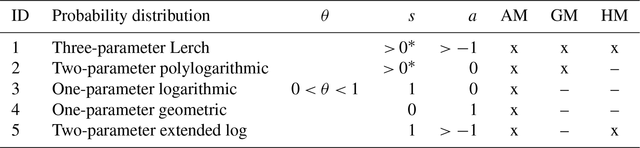
* The condition s>0 allows a monotonically decreasing pmf to be obtained, with a mode equal to 1.
This distribution makes it possible to account for some peculiar characters observed in the it samples, such as high values of both standard deviation and skewness, a monotonically decreasing pattern of frequencies with a slowly decaying tail, and a typical “drop” entering the dry status (it = 2) from the wet status (it = 1).
To estimate the parameters of the Lerch distribution, the maximum likelihood estimation (MLE) method was applied. For the general case (three-parameter, Eq. 1), the analytical solution of the MLE method returns arithmetic, geometric, and harmonic expectations equal to the corresponding sample values. If N denotes the sample size, the MLE function reads as (Gupta et al., 2008)
For each special case of the family of Lerch distributions, Table 1 also reports the constraints that need to be satisfied in the MLE. The likelihood equations were solved for both the DM and IM by standard numerical methods to obtain the MLE.
While the general three-parameter form (ID = 1 in Table 1) fits at least as well as any special cases with a smaller number of parameters (ID = 2–5 in Table 1), the inclusion of additional parameters is not always statistically justified (Wilks, 1938). For this reason, the likelihood-ratio (LLR) test was employed to detect whether the improvement in terms of log-likelihood is worth the introduction of the extra parameters. In this test, the D statistic was computed from the log-likelihood of the null model (ln(LID) with ID = 2–5) and of the alternative model (ln(L1)) as
where both log-likelihood values are computed from Eq. (3) using the corresponding parameterization. The D values are approximately χ2-distributed, with degrees of freedom equal to the difference between the number of free parameters of the alternative and null models.
To assess the adequacy of the Lerch family distribution in reproducing the observed frequencies, we employed a simulated χ2 goodness-of-fit test. When the distributions exhibit a long tail, the classical χ2 test might be biased due to the presence of numerous small class sizes (with fewer than five elements) and strong asymmetry (Martínez-Rodríguez et al., 2011). Therefore, we proceeded by reconstructing the distribution of the χ2 statistic under the null hypothesis via Monte Carlo simulation (Hope, 1968). Let us remind the reader that this well-known goodness-of-fit test is characterized by the null hypothesis that the data follow the specified distribution and by the alternative hypothesis that the data do not follow the specified distribution.
We simulated 3000 replicates of the sample by random sampling from the inferred theoretical distribution. The associated p value (at a significance level of 0.05) was computed as the fraction of the 3000 replicates for which the computed values (with ) were greater than , i.e., the χ2 of the observed frequencies.
2.2 Inference of the main time properties of rainfall series
Let a time series of rainfall data be defined as , where h (mm) is the rainfall depth recorded at a fixed uniform unit τ of time (e.g., a day). A day k is considered rainy if the rainfall depth , where h∗ is a fixed rainfall threshold. Thus, a subseries of rainfall depth h is selected from H, corresponding to the times such that with , and nr<n is an integer multiple of the timescale τ.
The interarrival time series it ={it1, it2, …, it is defined as the sequence built with the times elapsed between each element of E (except the first one) and the immediately preceding one. It is worth noting that, if itk=1, the rainy day k immediately follows the rainy day k−1; consequently, in the it time series, any sequence of m consecutive unitary values is a wet spell (ws) of duration m+1. Keeping in mind this observation, the isolated rainy day k is identified if the following condition is satisfied:
Additionally, the sequence of dry spells (ds) can be derived from the it sequence as
We define a “wet chain”, wch, as the sequence of wet spells broken by 1 d dry spells. This concept was introduced in Baiamonte et al. (2019), i.e., “wet day sequences”, and it corresponds to a ws if no interruption occurs, whereas, if an event ds > 1 occurs, the wet chain runs out. Similarly, here we introduce a “dry chain”, dch, a sequence of dry spells interrupted by 1 d wet spells. A dch corresponds to a ds if no interruption occurs, whereas a dch expires if ws > 1 occurs. Different examples of wch and dch are given in Fig. 1.
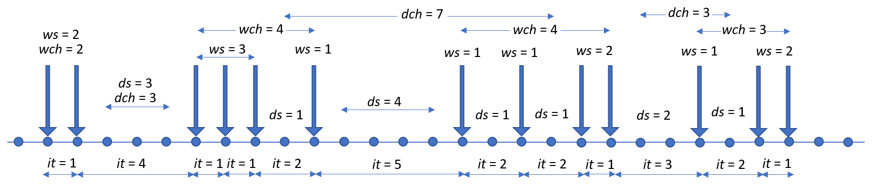
Figure 1Examples of interarrival times (it), wet spells (ws), dry spells (ds), wet chains (wch), and dry chains (dch).
From a hydrological point of view, the above-described wch can be seen as a single rainy period in a broad sense, since a single non-rainy day in between multiple rainy days does not significantly alter the wet status, as if the entire period is likely related to the same meteorological perturbation. A similar consideration can be made for dch, since a single rainy day that interrupts a sequence of dry spells may also not significantly alter the dry status, with the additional caveat that the rainfall depth during the isolated rainy day should be a limited amount. Following the consideration that an isolated rainy day (surrounded by two dry spells) is likely associated with only a few hours of rain, the assumption of limited rainfall depth seems reasonable when only durations are analyzed.
2.2.1 The direct method
According to previous studies (Agnese at al., 2014; Baiamonte et al., 2019), a direct inference on the it pmf (from now on referred to as the DM) can be performed by Eq. (1) (with v= it). Following the i.i.d. hypotheses on it, the resulting random variable ws is were geometrically distributed with parameter (1−pit(1)), where pit(1) is the probability that it is equal to 1 as given in Eq. (1). Thus, we have
where pit(1) is equal to
From Eq. (7), the ws pmf satisfies the memoryless property of the geometric distribution, i.e.,
Equation (9) is a consequence of the simple but restrictive hypothesis that the probability of future rainy day occurrence is not affected by the occurrence of past rainy days; i.e., the probability of a rainy day is assumed to be constant (Chatfield, 1966).
According to Eq. (6), the ds pmf can be easily recovered from the it pmf as (Agnese et al., 2014)
The wch pmf follows from the it distribution by also considering that a wet chain is a sequence of it = 1 (consecutive rainy days) and it = 2 (corresponding to a hole in between 2 rainy days), ending with it > 2. Therefore, taking into account the probabilities that it is equal to either 1 or 2 as well as all the probability of different combinations of it values, we can write
where j () is the number of holes breaking the wet status, is the number of subsets of j elements chosen among k−1 elements, and is the number of it = 1, indicating a wet spell of size k−1. It is worth highlighting that .
An alternative, and more general, formulation of wch pmf, pwch(m), relies on a convolution approach. In this case, pwch(m) can be obtained following two observations: (i) that the probability of the sum of k wet spells of any duration (, with ) is equal to the k-fold convolution of ws with itself, corresponding to ; and (ii) that the probability of having a sequence of k−1 1 d dry spells, corresponding to , can be expressed as . By extending the convolution over all the possible combinations of ws sequences, summing to m and to the n 1 d ds sequences () breaking the wet status, the probability pwch(m) can be expressed as
Equation (11) follows from Eq. (12) when the hypothesis of i.i.d. on renewal times it holds.
Using similar arguments but with ds in place of ws, the dch pmf, pdch(m), results in
which can be obtained from Eq. (12) by simply substituting ws with ds and vice versa. Note that pdch(1)=pds(1) (1−pws(1)). It should be observed that the definition of chains can be easily extended to interruptions longer than a single day (i.e., a 2 d wch is a sequence of it = 1, it = 2, and it = 3, ending with it > 3). However, the chains can become less and less realistic with increasing length of the interruption.
Equations (7), (10), (11), (12), and (13) show that in the DM the probability distributions of the wet and dry spells and of the wet and dry chains can be directly recovered from the it distribution, without the need for extra fittings or parameterizations.
2.2.2 The indirect method
The IM is based on modeling individually the random variables ws and ds, and it is the most commonly adopted approach for the modeling of ws and ds in hydrology (Kottegoda and Rosso, 2008). Both distributions rely on Eq. (1) (v= ws and v= ds). In this case, the observations of ws and ds are assumed to be i.i.d. and independent of each other. Note that, contrary to what has been observed in many studies and described in Sect. 2.2.1, in the IM the ws distribution is not constrained to be geometric, since the hypothesis of constant probability – when a wet day is followed by another wet day – is removed. Indeed, we have
where the left-hand-side term is the so-called failure rate, FRws(r). If the ws pmf is assumed to belong to the family of Lerch distributions, the failure rate reads as (Gupta et al., 2008)
If we set s=0, which corresponds to Geom(1−θ) in the family of Lerch distributions (Table 1), we get FRws(r)=θ, and thus is constant, as expected. For all the other distributions in the Lerch family, FRws(r) will suitably depend on r allowing for more flexibility (Gupta et al., 2008).
Once both the ws and ds distributions are known, the it distribution can be easily recovered as
The procedure to derive it from ws and ds is not commonly discussed in studies adopting the IM method, as they are usually focused only on the modeling of ws and ds rather than it.
As in the DM, the probability distribution of wch and dch can be obtained from Eqs. (12) and (13), respectively, where the probabilities pds and pws are now separately inferred, unlike in the DM, for which these probabilities are recovered from the it distribution. It is worth mentioning that, for the wch pmf, Eq. (11) is no longer valid, since the assumption of a memoryless property is relaxed. From a computational point of view, we emphasize that the IM will always require two fittings (ws and ds) performed through a numerical MLE, unlike the DM, where only one fitting is sufficient to recover the distribution of it.
3.1 Rainfall records
In this paper, to obtain the series of rainfall time variables (it, ws, ds, wch, dch), daily rainfall records are analyzed. To discriminate between rainy and non-rainy days, a fixed rainfall threshold mm is chosen according to the conventional value established by the World Meteorological Organization. The dataset includes six time series collected over Europe at different latitudes (from 38 to 58° N), from Trapani and Floresta in Sicily to Stornoway in northern Scotland. Figure 2 depicts the spatial location and altitude of the six stations. About 70 years of recorded data are used for each rain gauge: Ceva (1950–2016), Floresta (1951–2015), Oxford (1950–2017), Stornoway (1950–2020), Torino (1950–2017), and Trapani (1950–2015), with a minimal occurrence of missing data.
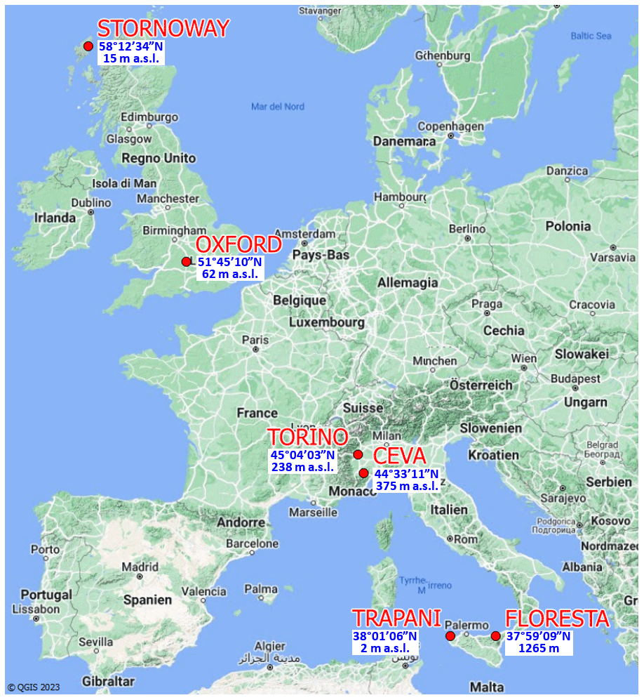
Figure 2Locations of the six considered stations, together with latitudes and elevations above sea level (© QGIS 2023).
Due to the relevance of rainfall regimes for the distribution of rainy and non-rainy days, in addition to the analysis of the entire year (Y), all the analyses were performed for two additional data subsets: (S1) from April to September and (S2) from October to March.
The analyzed stations are characterized by different rainfall regimes, as shown in Fig. 3 by the average number of rainy days in each month (panel a) and the fraction of the yearly-average rainy days in each month (panel b) (as a standardization of the data in panel a). The stations of Trapani (TRA) and Floresta (FLO) represent the typical Mediterranean climate, with a strong seasonality in the rainfall regime (see Fig. 3b) and precipitation concentrated in the S2 season. The two stations differ in the total amount of average annual rainfall, which is low for TRA (420 mm) and high for FLO (1133 mm), a difference that is also revealed by the different number of rainy days per month (Fig. 3a). Torino (TOR) and Ceva (CEV) are characterized by a mid-latitude sublitoranean climate with a high rain frequency in spring (Fig. 3b). CEV also exhibits a secondary peak in autumn, mainly due to the influence of the Tyrrhenian Sea warming in summer. Despite this difference, the two stations are characterized by a similar total annual rainfall (829 and 836 mm, respectively) and number of rainy days (Fig. 3a). Oxford (OXF) is a northern European station with a relatively low average rainfall amount (592 mm) homogeneously distributed throughout the year, whereas Stornoway (STW) has a very high rain frequency and a higher amount all through the year (1072 mm) due to its location in far northwestern Scotland and the direct effect of the wet fronts from the Atlantic Ocean. Both stations in the UK have low seasonality compared to the other stations (see Fig. 3b).
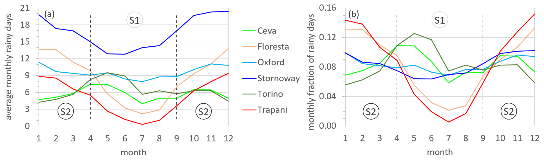
Figure 3Time variability of (a) the average number of rainy days in each month and (b) the fraction of yearly-average rainy days in each month. Dashed lines delimit the two seasons S1 (April–September) and S2 (October–March).
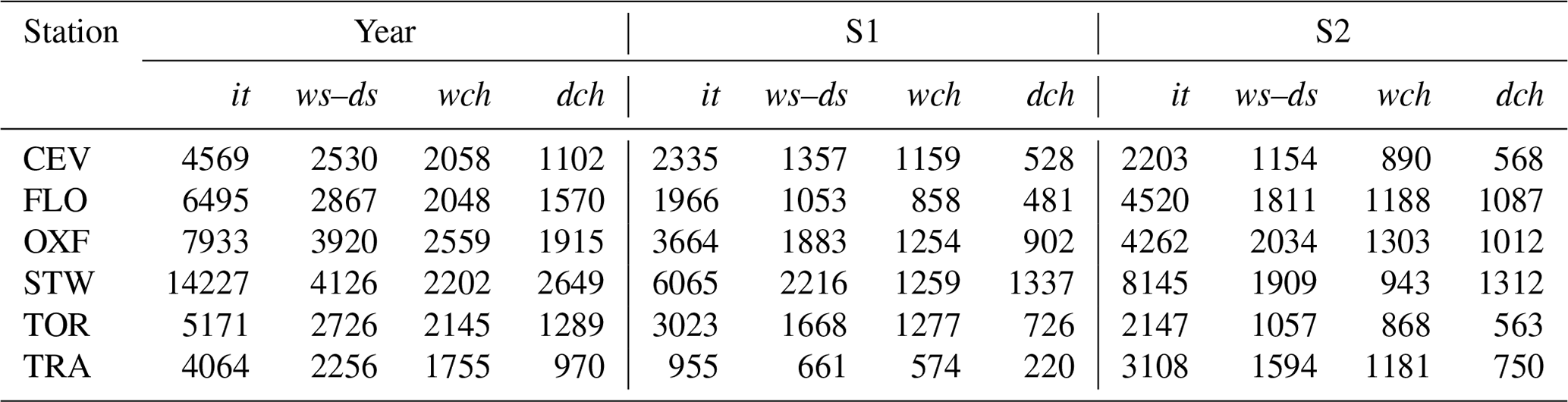
For the TRA and FLO stations, seasons S1 and S2 clearly correspond to the low and high frequencies of rain events, respectively (Fig. 3b). A similar pattern can be observed for OXF and STW, although with less marked differences between the two seasons. Due to the considerable length of the data records, sample sizes remain large even for the two seasonal datasets, as summarized by the data in Table 2. The sample size is less than 500 only for dch in TRA for S1, which can be explained by the numerous long dry periods occurring in the dry season.
Table 2Sample sizes of the time variables for the six stations and for the three periods Year, S1 (from April to September), and S2 (from October to March).
It is noteworthy that the splitting of the two seasons of CEV and TOR was done differently in a previous paper (Baiamonte et al., 2019). However, in this paper the same splitting into two 6-month seasons is used for the sake of the homogeneity of the present analysis (Fig. 3a and b).
3.2 Preliminary tests on observed records
As is well known in the literature, the presence of a trend in the datasets can affect the assumptions made for it (in the DM) or for ws and ds (in the IM). Therefore, before fitting, a trend test was performed. We used the well-known Mann–Kendall (MK) nonparametric test (Mann, 1945; Gilbert, 1987) at a significance level of 0.05. Note that the MK test is frequently used in the literature to detect significant trends in hydrometeorological time series (see, e.g., Gocic and Trajkovic, 2013, and references therein).
However, a known limitation of the MK test is the increased probability of finding trends in the presence of a significant autocorrelation in the data (Hamed and Rao, 1998). In such a case, the variance of the MK test statistic depends on the true unknown autocorrelation structure, and it is typically larger (lower) if positive (negative) autocorrelation occurs with respect to the case of independent data. Therefore, in the presence of autocorrelation, a correction is needed, as the critical values of the classical MK test would lead to incorrect results. Hamed and Rao (1998) proposed an approximation of the true variance of the MK test statistic in the case of autocorrelated data.
Let us recall that a key difference between the DM and the IM, as introduced in Sect. 2.2, is related to modeling the it samples as i.i.d. renewal times, which results in a geometric distribution of ws in the DM. One way of directly testing the memoryless property of the empirical data is to study the behavior of the ratios for all , with Sr the number of wet spells of length at least r in a ws series. The memoryless property implies that these ratios are constant, while they would depend on r for a pmf in the general form of the Lerch distribution (Gupta et al., 2008).
4.1 Nonparametric analyses
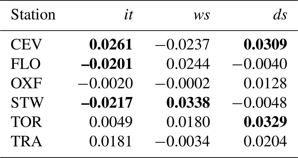
The presence of a trend on the recorded it, ws, and ds time series was tested using Kendall's τ, which is a nonparametric measure of rank correlation. The standard MK test – applied using the τ values reported in Table 3 – shows the presence of a small statistically significant trend in some cases (indicated in bold in the table). Since a weak positive autocorrelation was always observed (Table 3) for the three variables it, ws, and ds at each of the six stations, the corrected MK was implemented through the Fume package of the R software (2012). This corrected test returned the absence of a statistically significant trend for all the variables and stations; therefore, the entire dataset can be adopted for subsequent analyses.
Table 3Values of Kendall's τ statistic for the Year period time series of the six stations. In bold are the values that are statistically significant (p=0.05) for the classical MK test but not for the corrected MK test. All the other values were found to be not significant, even with the classical MK test.
To verify the memoryless property of ws directly on the empirical data, Fig. 4 plots the sequence of the ratio for all the stations and periods. The series are reported up to ws values with a number of observations greater than or equal to 10. These results show a roughly constant value for the two stations of CEV and TOR (Fig. 4a), a slightly increasing trend for TRA and FLO (Fig. 4b), and a marked increasing trend for OXF (Fig. 4c) and STW (Fig. 4d). These results suggest that the use of a geometric distribution for the ws records of OXF and STW may not be adequate, as successively investigated with the parametric analysis, since the variability of the ratios could be considered a rough indicator of the inadequacy of the geometric distribution in describing wet spells (Chatfield, 1966).
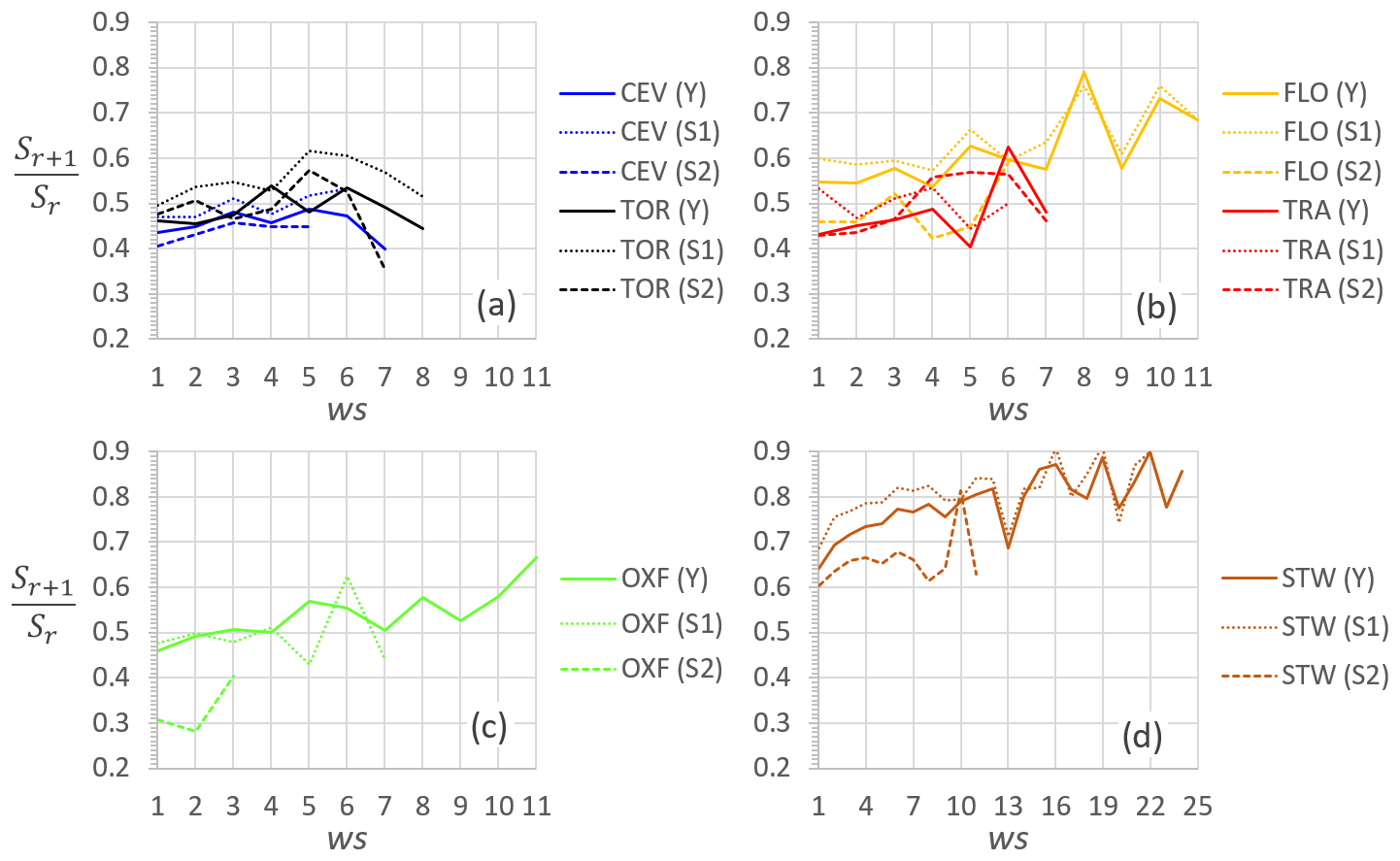
Figure 4For the three periods Y, S1, and S2, the ratio versus ws (a) for CEV and TOR, (b) for FLO and TRA, (c) for OXF, and (d) for STW.
The main statistics of all the rainfall time variables, it, ws, ds, wch, and dch, are summarized in the box plots depicted in Fig. 5, reporting the statistics for all the stations and for the three periods Y, S1, and S2. The figure highlights the different statistical characters of the investigated variables and how the seasonality seems to affect all the sites.
It is interesting to observe that the STW station shows the highest ws and wch statistics, likely due to its high-frequency rainfall. These high values are obviously counterbalanced by the lowest it, ds, and dch statistics for all the considered periods. For ws (S1), almost all the stations show a quite limited range of variability, with the exception of STW and TRA, which present very different rainfall regimes.
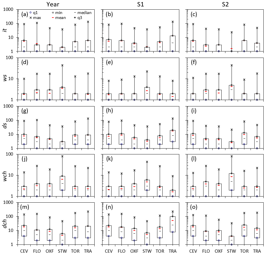
Figure 5Box plots of the statistics of time variables it (a–c), ws (d–f), ds (g–i), wch (j–l), and dch (m–o) for all six stations and for the three periods Year (left column), S1 (central column), and S2 (right column). The variables q1 and q3 identify the first and third quartiles, respectively.
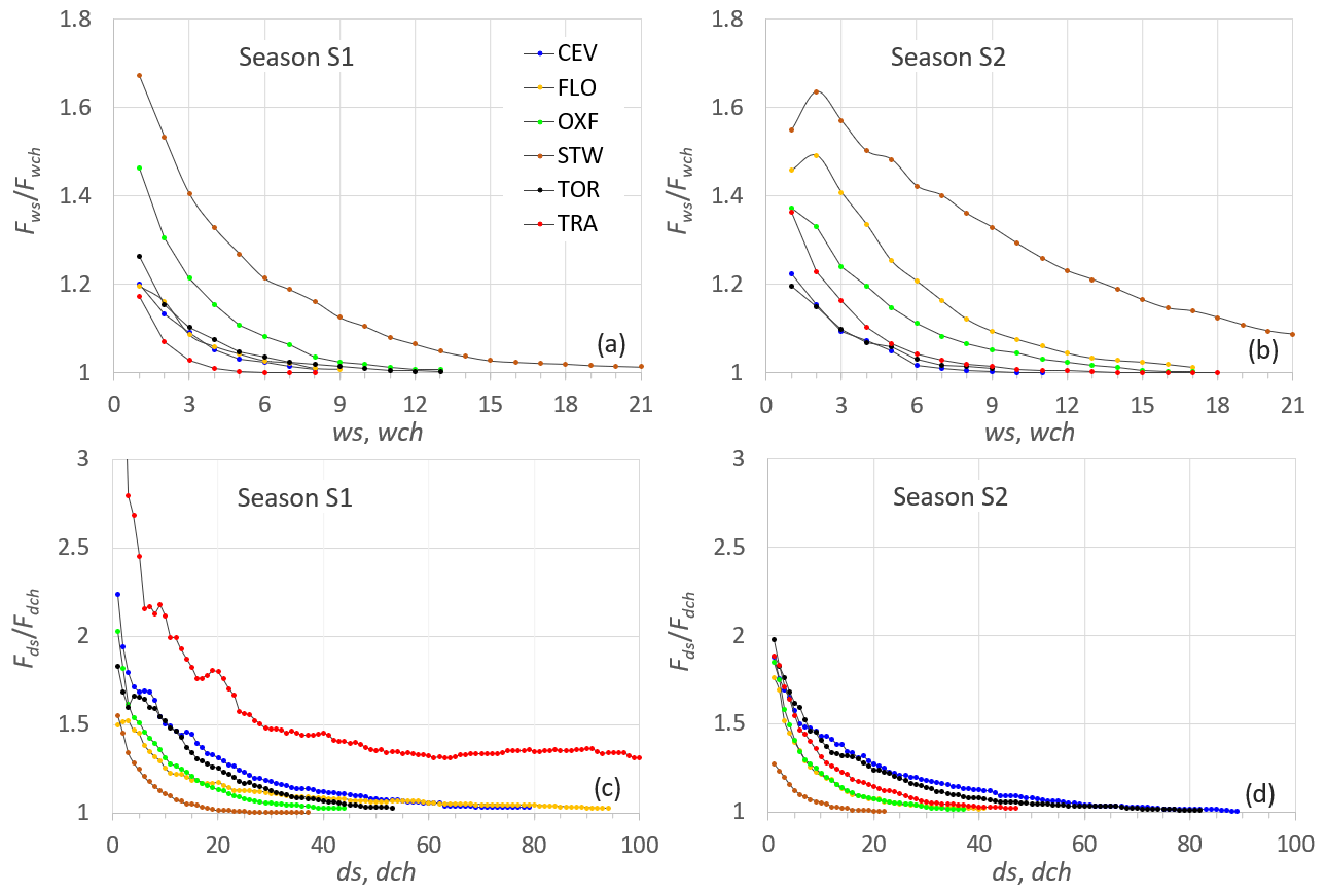
Figure 6Ratios between observed cumulative frequencies (a, b) and (c, d) for the six stations and for S1 (a, c) and S2 (b, d).
In-depth analysis of the relationship between spells and chains can be made of the data reported in Fig. 6, where, for the six stations and for the two seasons S1 (a, c) and S2 (b, d), the ratios of the observed cumulated frequencies (a, b) and (c, d) versus the corresponding time variables are plotted. These ratios describe the relative weight of the derived variable dch (wch) on ds (ws). As expected, the ratios and are greater than unity, with larger values for [1–3] than for [1–1.7]. In general, moving from S1 to S2, higher and lower values can be observed. Ratios corresponding to the CEV and TOR rain gauges provide almost similar values for the two seasons according to the limited seasonality, whereas STW, characterized by a very high rainfall frequency, is the only case with a ratio higher than . Finally, it is worth noticing the very high values of for TRA in the S1 period, reflecting the aridity that characterizes the area of western Sicily during that season and the large differences in in FLO when comparing the two seasons.
4.2 DM and IM comparison
For the time series of the six rain gauges, the Lerch family (as given in Eq. 1) was fitted on the three periods (Y, S1, and S2) for it (DM) and for both ws and ds (IM). The parameters obtained by MLE are summarized in Table 4. It is important to highlight that, for each station–period combination, the parameters reported in Table 4 correspond to the Lerch family special cases (see Table 1), as supported by the results of the LLR test (e.g., three parameters are adopted only when this number of parameters is justified by the test).
Table 4Parameters of the Lerch family of probability distributions fitted on it (DM) as well as ws and ds (IM) for the six stations and for the three periods Year, S1, and S2. Values of 0 or 1 for parameters s and a identify the special cases listed in Table 1.
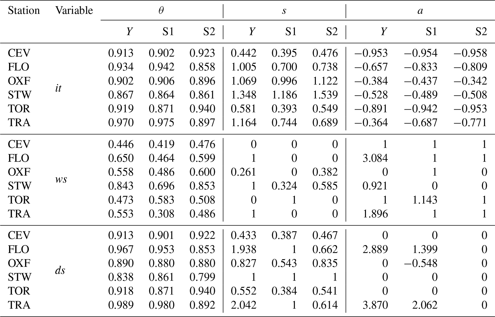
In the case of it (DM), the three-parameter Lerch distribution is selected for all the sites and periods; the θ parameter varies between 0.86 and 0.97, with higher values observed for the whole year and season S1 for TRA. The variation of θ in the various periods is very limited for OXF, STW, and to a lesser extent CEV, as evidenced by a low degree of seasonality compared to the other stations. As expected, the a values are all negative (Table 4), since the a parameter allows the observed drop in frequency to be reproduced when moving from it = 1 to it = 2. The s parameter is positive for all the it fittings, suggesting that the mode is always at it = 1.
For the IM, the geometric distribution (s=0 and a=1) was chosen in several cases (10 out of 18) to fit ws, most commonly over the sub-seasons (8 out of 12) than over the whole year. The CEV station is the only one where the geometric distribution was selected for all three periods, while the geometric distribution was never selected for STW. To capture the probabilistic law of ws, OXF and STW seem to require the polylog series or the two-parameter extended log-series distribution (Table 1). It is interesting to observe that, for TRA and FLO, the geometric distribution is not appropriate for ws when the period is the year, while it is selected when the complete dataset is split into two sub-seasons.
Concerning the ds distribution in the IM, two or three parameters are always required, with the notable exception of STW, where the logarithmic distribution (s=1 and a=0) is selected for all three periods. The polylog-series distribution is selected for 10 out of 18 cases, confirming the adequacy of this distribution for describing the probability law of dry spells in different cases; notably, for CEV and TOR the values assumed by θ and s in the polylog distribution of ds are almost equal to those of the Lerch distribution for it. Hence, for these stations, the additional parameter a in the Lerch distribution fulfills, in practice, the function of accounting for the geometric distribution of ws.
The assessment of the goodness of fit for the selected distributions (for it in the DM and for ws and ds in the IM) is synthetically illustrated in Fig. 7. In particular, for all the stations and periods (Y, S1, S2), the computed p values are classified according to four ranges (0–0.01, 0.01–0.05, 0.05–0.1, and 0.1–1), with light (0.05–0.1) and dark (0.1–1) green classes referring to the acceptance range of the null hypothesis. For a few of the 180 (6 stations × 3 periods × 5 variables × 2 methods) Monte Carlo procedures (19 out of 180), the presence of outliers (high values with a very low frequency) suggested preliminary data smoothing. Such smoothing was performed by uniformly distributing the frequency of the outlier over all the values between the observed value and the latest observed non-null frequency. In Fig. 7, these cases are marked by black dots. Overall, Fig. 7 shows that the fitting of it is satisfactory in all the cases for Y, with only one exception (FLO) with a p value just above 0.05. Analogously, good results are obtained for ds, which is not surprising given the close relation between it and ds modeling in the DM framework (see Eq. 6). In contrast, the fits are not satisfactory in several cases for the resulting ws and wch, most notably for STW and TRA.
The data depicted on the right-hand side of Fig. 7 (i.e., IM) suggest that, when the IM is applied, there is a significant reduction in the number of unsatisfactory fits (red and orange classes), particularly for ws and wch. In addition, when analyzing the seasonal datasets, a further improvement in the identification of the probability law of the time variables is evident.
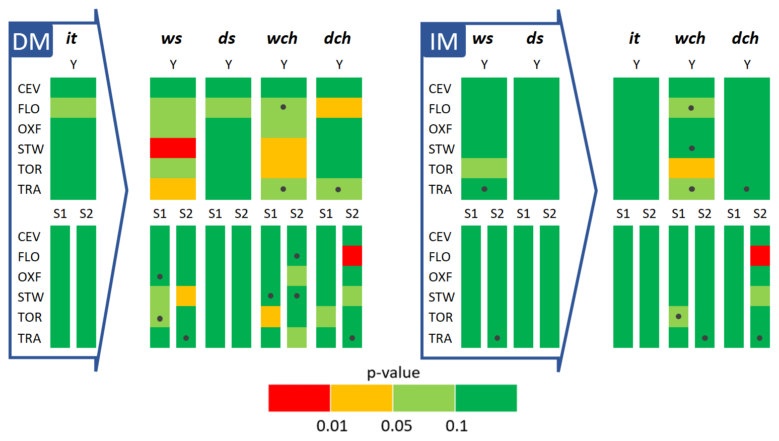
Figure 7Summary of the results of the χ2 test for both the direct (DM, a) and indirect (IM, b) methods. The variables inside the large arrows are the ones fitted in the corresponding method, whereas the other variables are deducted. The p values (see the legend) for all the stations and periods are reported. The black dots indicate that smoothing of the observed frequencies was applied to calculate .
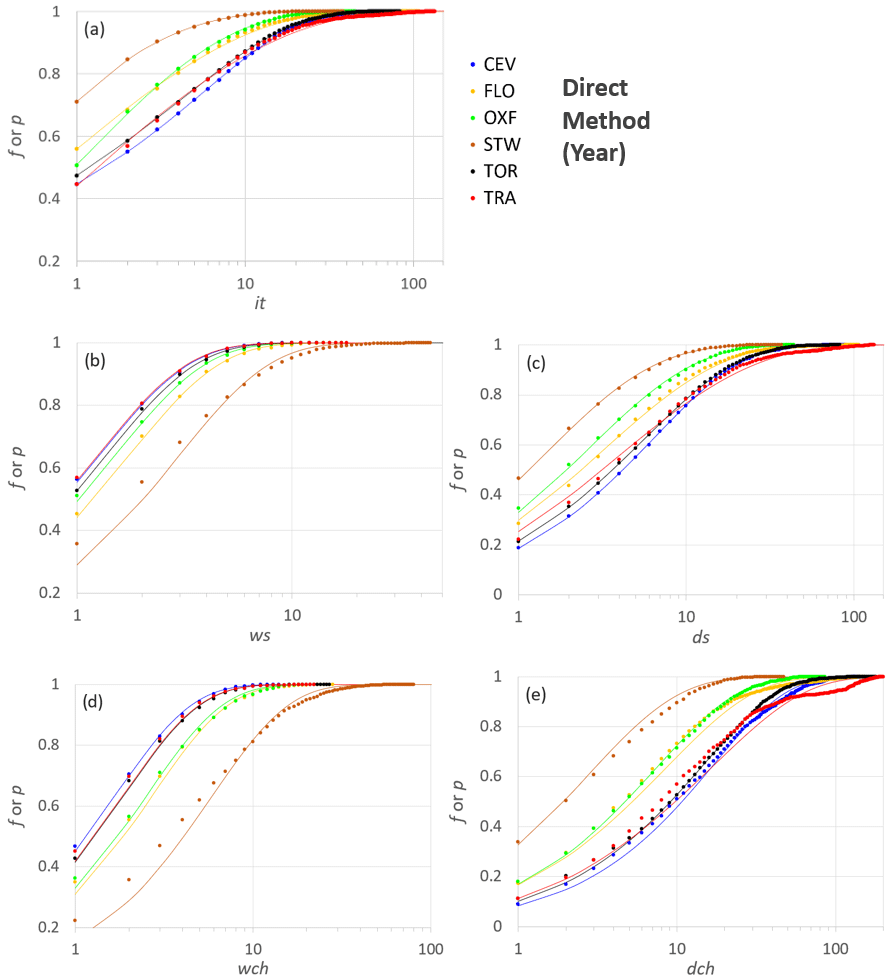
Figure 8Observed frequencies and fitted probability distributions for the six stations according to the DM and for the period “Year”. The variables on the x axis are in logarithmic scale.
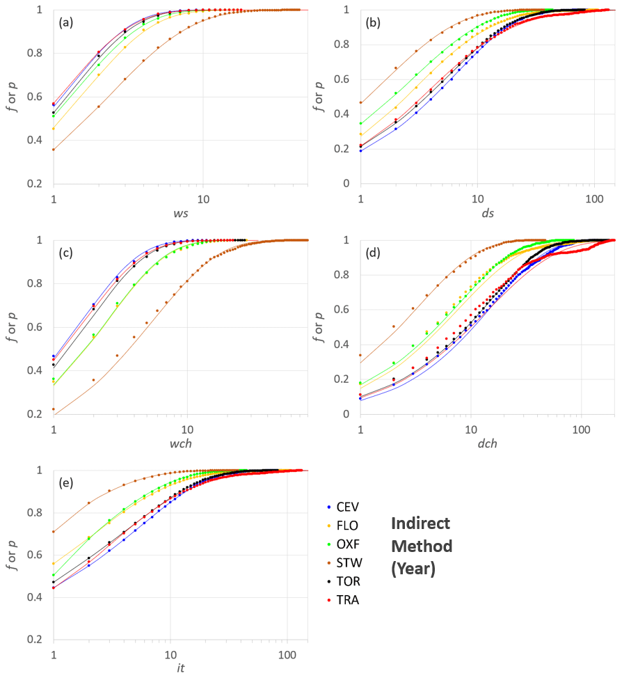
Figure 9Observed frequencies and fitted probability distributions for the six stations according to the IM and for the period Year. The variables on the x axis are in logarithmic scale.
The plots in Figs. 8 and 9 show the cumulative observed frequencies and the corresponding fitted Lerch family probability distributions for the annual period (Y) when applying the DM and the IM, respectively. The comparison between the two methods confirms the overall net improvement achieved by the IM in those cases that were not well fitted in the DM, such as ws and wch for STW (compare Fig. 8b and d with Fig. 9a and c). The latter consideration is also supported by the comparison between the p value classes (Fig. 7) associated with the same variables, when the IM is used in place of the DM. This result underlines how the i.i.d. hypothesis for it in the DM may not always be valid.
Since the previous results show that the main difference between the two methods concerns the ability to model ws and wch and to a lesser extent dch, the plots in Fig. 10 depict the difference in the cumulated frequencies for these variables modeled through the two methods for S1 (panels a, c, e) and S2 (panels b, d, f), respectively. These results further emphasize how the IM improves the performances in most of the cases given the high fraction of points located in the portion of the plots below the 1:1 line (i.e., differences in the DM are larger than in the IM). Overall, most of the differences lie along the identity line, suggesting good performance for both methods but with large discrepancies observed for STW, OXF, and FLO, i.e., for the cases in which the renewal property needs to be relaxed.
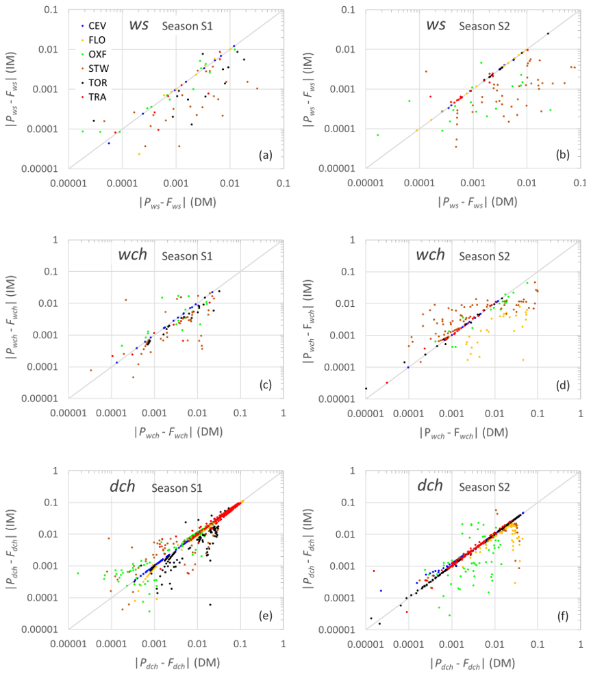
Figure 10Scatterplots of the absolute difference between observed frequencies and fitted probabilities with the DM (x axis) against the IM (y axis) for ws (a, b), wch (c, d), and dch (e, f).
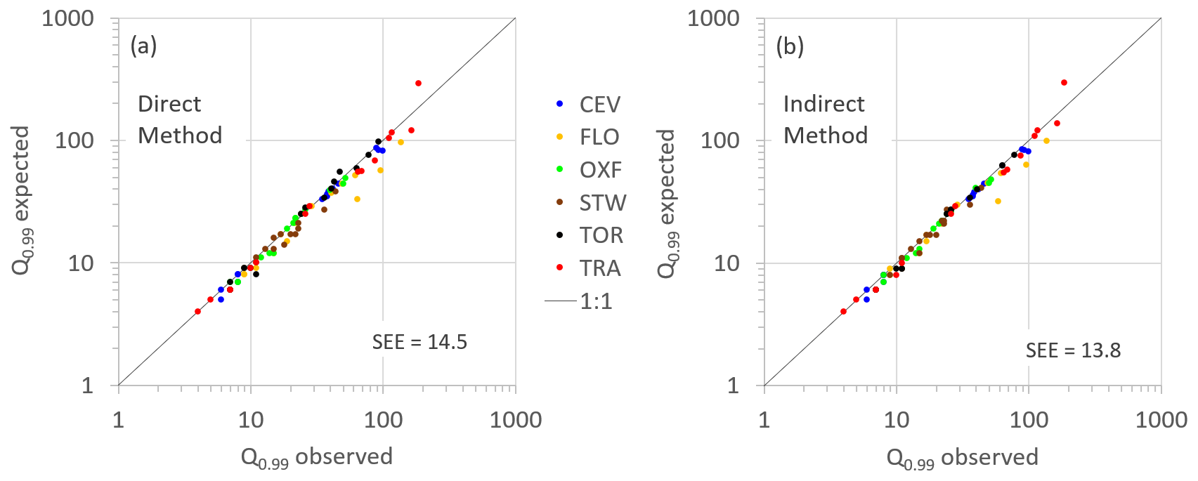
Figure 11Comparison between the empirical and theoretical quantile Q0.99, calculated according to the DM (a) and the IM (b) for all the stations, periods, and time variables bundled together.
The Lerch family distribution also allows the probability of extremes of the time variables to be predicted. The overall consistency of the latter can be observed in Fig. 11, where the empirical 99th percentiles, Q0.99, are compared with the estimated ones, for all stations and periods, when applying the DM (Fig. 11a) and the IM (Fig. 11b). Figure 11a shows that the dots are quite close to the line of perfect agreement, with only a few exceptions likely due to the limited sample size, as for the Sicilian stations for season S1. A slight improvement can be obtained by applying the IM, as shown by the decrease in the standard error of the estimate (SEE) reported in the figures. These results suggest that the poor performances observed for the DM is some cases do not significantly affect the results on the tails but only the accuracy in the most frequent data.
The fitting of the Lerch distribution to the selected six stations extends the studies previously carried out for the stations in Sicily and Piedmont (Agnese at al., 2014; Baiamonte et al., 2019). The adequacy of this distribution in fitting it is confirmed when data recorded over OXF and STW are considered, despite the rather different rainfall patterns of these latter stations compared with those previously analyzed. Most notably, the observed frequencies for it are already well reproduced at the annual scale, stressing how splitting the datasets into subperiods is not strictly necessary for correctly reproducing the probabilistic law of it in any of the rainfall regimes under consideration. The scientific literature on the statistical inference of rainfall interarrival times is still rather sparse, so further evidence of the suitability of the Lerch family for reproducing it distributions in a wide range of rainfall regimes is encouraging for further applications of the methodology.
However, the results obtained for ws and ds with the DM highlight how a good fit of it does not necessarily guarantee a satisfactory reproduction of the frequency of these derived quantities and, in particular, how the geometric distribution is not always adequate in describing wet spells. The ability to better reproduce the observed frequencies of ws with the IM and thus with distributions relaxing the memoryless property suggests the presence of an inner structure in multiday rainfall events, which manifests in a non-constant rain probability within the event itself. Usually, the internal structure observed in subdaily (e.g., 10 min) rainfall records is assumed to vanish at the daily aggregation steps (e.g., Ridolfi et al., 2011), but the results reported here may contradict this assumption at some of the investigated sites.
The need to resort to a more complex distribution than the geometric one to reproduce the probabilistic structure of ws has been highlighted in the literature, especially for long spells, by the studies of Berger and Goossens (1983) for rainfall data in Belgium and Deni and Jemain (2010) in Malaysia. The inadequacy of the geometric distribution is confirmed here for long ws (> 10 d) with a relatively high frequency, such as the case of STW where the DM returned poor performances. It is important to underline how the unsatisfactory fitting of a geometric distribution may not necessarily translate in the presence of memory in the rainfall series. In this regard, on the one hand, the results observed for the stations of TRA and FLO may suggest other reasons behind the poor performance of the geometric distribution in modeling ws as derived from it. The geometric distribution seems to be a suitable choice when the data are analyzed separately for the two seasons, which might imply that the complex structure of the ws distribution observed over the entire year is not associated with an actual relaxing of the renewal property but with a mixing of ws samples collected during two rather distinct seasons.
On the other hand, the geometric distribution seems to perform poorly on STW regardless of seasonality, which is actually quite limited for this station. The STW station seems to represent a case where the memoryless property is violated, as also confirmed by the inspection of the ratios.
Splitting the entire dataset into subperiods seems to improve the performance of fittings crosswise for both the DM and the IM. This result is well suited for possible implementations of the methodology for operational applications related to ecohydrology models (e.g., D'Odorico et al., 2000; Petrie and Brunsell, 2011) and stochastic weather generators (e.g., Paek et al., 2023). In these fields, to express the climatic component of weather variables (Semenov et al., 1998), not only does the overall probabilistic structure of rainfall need to be reproduced, but information on a seasonal or even subseasonal (i.e., monthly) scale is also required. Other studies, carried out over regions characterized by a climate with no distinct monsoon seasons, have also highlighted the importance of focusing on either the dry summer seasons or wet winter seasons (Caloiero and Coscarelli, 2020; Paton, 2022; Raymond et al., 2016). Wan et al. (2015) also suggested the need to account for the seasonality to properly reproduce the duration of ws for Canada using a Markov chain method.
Another consequence of the inadequacy of the geometric distribution in describing wet periods is that the daily structure of rainfall needs to be taken into account for modeling processes such as the seasonal dynamics of soil moisture and vegetation. Ratan and Venugopal (2013) did an assessment for tropical areas using satellite rainfall data. They found wet spell durations with a peak at 1 d for dry regions, while the duration of 2–4 d is predominant for humid areas. A similar but reversed observation was made for dry spells, resulting in 1 d for humid areas and 3–4 d for dry areas.
For some cases, the results obtained for the IM suggest that the classical application of the geometric distribution for ws and of the polylog series for ds provides satisfactory modeling of the observed frequencies. However, there are no substantial benefits to using these two distributions over using a three-parameter Lerch distribution. Indeed, a similar number of fitting parameters is required in the DM and IM but with the obvious drawback of having an increasing computational cost due to the need to perform two independent fittings (for ws and ds) compared to a single one (it only). In this context, the case of STW is peculiar, where the geometric distribution is never selected for ws and a two-parameter distribution is always required, although a one-parameter distribution is used at this site for ds. This circumstance suggests that a reliable fit of the two quantities can still be achieved without increasing the total number of parameters when compared with the three-parameter Lerch.
Finally, it is worth mentioning that the models proposed in this paper are local, and hence spatial dependency in parameters may need to be accounted for in applications to multiple stations located at shorter distances.
In this paper, daily rainfall data belonging to a large range of rainfall regimes across Europe (latitudes 38–58° N) have been analyzed to model the frequency distribution of some key rainfall time variables. By using two different methods, the assumption of the renewal property that implies the geometric distribution of wet spells has been investigated. First, a direct method (DM), where the geometric distribution of wet spells is assumed, has been applied. Second, the latter assumption is relaxed by using an indirect method (IM) where wet spells and dry spells were modeled separately, hence including the possibility of accounting for a non-constant rain probability inside the rainfall cluster.
As a general rule, the results of comparing the DM and the IM suggest that the Lerch distribution can be successfully used for both interarrival times and dry spells in a wide variety of rainfall regimes, whereas a preliminary analysis of the memory property (e.g., of the ratios) may be needed to assess the reliability of the wet spells derived from the interarrival times modeled with the DM using the Lerch family. When signals of memory are detected, the IM is recommended, as it is better suited for a wider range of conditions, albeit with a potentially larger number of fitting parameters.
The analysis was extended to include two additional time variables strongly associated with wet and dry spells, referred to as wet and dry chains. These variables extend the concept of wet and dry spells to sequences characterized by an interruption of 1 non-rainy day or 1 rainy day, respectively, as they represent two quantities that may be of interest for practical hydrological applications. The results obtained for the two chains generally reflect the findings obtained for the spells, albeit highlighting additional difficulties in the probabilistic modeling, especially at sites where the sample size may become a limiting factor.
The effects of the seasonality on the results were also addressed, splitting the data into two 6-month subperiods. This separation tends to improve the performances for both the DM and the IM, stressing how at most of the sites the DM applied to seasonal data is still a suitable straightforward approach. The results of this study may help in scenario simulations of drought and flood events, considering that probabilistic functions, such as those applied in this work, are at the root of stochastic climate modeling.
Future research aimed at investigating the neighboring location effects on parameter values will be developed.
Codes used for this study can be shared upon request to the main author.
Data used in this analysis and outputs can be shared upon request to the corresponding author.
Conceptualization: GB, CA, CC, EDN, SF, TM. Data curation: GB, CA, SF. Formal analysis: GB, CA, CC, EDN, TM. Investigation: GB, CA, CC, EDN, TM. Methodology: CA. Validation: GB, CA, CC, EDN, TM. Visualization: GB. Writing – original draft preparation: GB, CA. Writing – review and editing: GB, CA, CC, EDN, SF, TM.
The contact author has declared that none of the authors has any competing interests.
Publisher's note: Copernicus Publications remains neutral with regard to jurisdictional claims made in the text, published maps, institutional affiliations, or any other geographical representation in this paper. While Copernicus Publications makes every effort to include appropriate place names, the final responsibility lies with the authors.
The authors would like to thank Nicholas Howden, School of Civil, Aerospace and Mechanical Engineering, University of Bristol, for providing the Oxford rainfall data, INDAM and especially the GNAMPA group for their support, and the anonymous reviewers and the editor for their valuable comments.
This work was supported by the PRIN MIUR 2017SL7ABC_005 WATZON project, PRIN2022PFKP Sunset, and by NODES, which received funding from the MUR-M4C2 455 1.5 of PNRR with grant agreement no. ECS00000036.
This paper was edited by Soutir Bandyopadhyay and reviewed by two anonymous referees.
Agnese, C., Baiamonte, G., and Cammalleri, C.: Modelling the occurrence of rainy days under a typical Mediterranean climate, Adv. Water Resour., 64, 62–76, 2014.
Baiamonte, G., Mercalli, L., Cat Berro, D., Agnese, C., and Ferraris, S.: Modelling the frequency distribution of inter-arrival times from daily precipitation time-series in North-West Italy, Hydrol. Res., 50, 339–357, 2019.
Berger, A. and Goossens, C.: Persistence of wet and dry spells at Uccle (Belgium), J. Climatol., 3, 21–34, 1983.
Bonsal, B. R. and Lawford, R. G.: Teleconnections between El Niño and La Niña events and summer extended dry spells on the Canadian prairies, Int. J. Climatol., 19, 1445–1458, 1999.
Caloiero, T. and Coscarelli, R.: Analysis of the characteristics of dry and wet spells in a Mediterranean region, Environ. Process., 7, 691–701, https://doi.org/10.1007/s40710-020-00454-3, 2020.
Chatfield, C.: Wet and dry spells, Weather, 21, 308–310, 1966.
Chowdhury, R. K. and Beecham, S.: Characterization of rainfall spells for urban water management, Int. J. Climatol., 33, 959–967, 2013.
Deni, M. S. and Jemain, A. A.: Mixed log series geometric distribution for sequences of dry days, Atmos. Res., 92, 236–243, 2009.
Deni, M. S., Jemain, A. A., and Ibrahim, K.: The best probability models for dry and wet spells in Peninsular Malaysia during monsoon seasons, Int. J. Climatol., 30, 1194–1205, https://doi.org/10.1002/joc.1972, 2010.
Dey, P.: On the structure of the intermittency of rainfall, Water Res. Manag., 37, 1461–1472, https://doi.org/10.1007/s11269-023-03441-z, 2023.
Dobi-Wantuch, I., Mika, J., and Szeidl, L.: Modelling wet and dry spells with mixture distributions, Meteorol. Atmos. Phys., 73, 2450-256, https://doi.org/10.1007/s007030050076, 2000.
D'Odorico, P., Ridolfi, L., Porporato, A., and Rodriguez-Iturbe, I.: Preferential states of seasonal soil moisture: The impact of climate fluctuations, Water Resour. Res., 36, 2209–2219, https://doi.org/10.1029/2000WR900103, 2000.
El Hafyani, M. and El Himdi, K.: A Comparative Study of Geometric and Exponential Laws in Modelling the Distribution of Daily Precipitation Durations, IOP Conf. Ser. Earth Environ. Sci., 12th International Conference on Environmental Science and Technology, 1006, 012005, https://doi.org/10.1088/1755-1315/1006/1/012005, 2022.
Gilbert, R. O.: Statistical methods for environmental pollution monitoring, Van Nostrand Reinhold Company, 334 pp., ISBN 0-442-23050-8, 1987.
Gocic, M. and Trajkovic, S.: Analysis of changes in meteorological variables using Mann-Kendall and Sen's slope estimator statistical tests in Serbia, Global Planet. Change, 1001, 72–182, 2013.
Green, J. R.: A generalized probability model for sequences of wet and dry day, Mon. Weather Rev., 98, 238–241, 1970.
Gupta, P. L., Gupta, R. C., Ong, S.-H., and Srivastava, H.: A class of Hurwitz–Lerch-Zeta distributions and their applications in reliability, Appl. Math. Comput., 196, 521–531, 2008.
Hamed, K. H. and Rao, A. R.: A modified Mann-Kendall trend test for autocorrelated data, J. Hydrol., 204, 182–196, 1998.
Hershfield, D. M.: A comparison of conditional and unconditional probabilities for wet- and dry-day sequences, J. Appl. Meteorol., 9, 825–827, 1970.
Hope, A. C.: A simplified Montecarlo significance test procedure, T. Roy. Stat. Soc. Ser. B, 30, 582–598, 1968.
Hughes, J. P. and Guttorp, P: Incorporating spatial dependence and atmospheric data in a model of precipitation, J. Appl. Meteorol., 33, 1503–1515, https://doi.org/10.1175/1520-0450(1994)033<1503:ISDAAD>2.0.CO;2, 1994.
Kottegoda, N. T. and Rosso, R.: Statistics, Probability, and Reliability for Civil and Environmental Engineers, McGraw-Hill, New York, NY, USA, 735 pp., ISBN 0070359652, 1997.
Mann, H. B.: Nonparametric tests against trend, Econometrica, 13, 245–259, 1945.
Martínez-Rodríguez, A. M., Sáez-Castillo, A. J., and Conde-Sánchez, A.: Modelling using an extended Yule distribution, Comput. Stat. Data Anal., 55, 863–873, https://doi.org/10.1016/j.csda.2010.07.014, 2011.
Osei, M. A., Amekudzi, L. K., and Quansah, E.: Characterisation of wet and dry spells and associated atmospheric dynamics at the Pra River catchment of Ghana, West Africa, J. Hydrol. Reg. Stud., 34, 100801, https://doi.org/10.1016/j.ejrh.2021.100801, 2021.
Paek, J., Pollanen, M., and Abdella, K.: A stochastic weather model for drought derivatives in arid regions: A case study in Qatar, Mathematics, 11, 1628, https://doi.org/10.3390/math11071628, 2023.
Paton, E.: Intermittency analysis of dry spell magnitude and timing using different spell definitions, J. Hydrol., 608, 127645, https://doi.org/10.1016/j.jhydrol.2022.127645, 2022.
Petrie, M. D. and Brunsell, N. A.: The role of precipitation variability on the ecohydrology of grasslands, Ecohydrol., 5, 337–345, https://doi.org/10.1002/eco.224, 2011.
Racsko, P., Szeidl, L., and Semenov, M.: A serial approach to local stochastic weather models, Ecol. Modell., 57, 27–41, 1991.
Ratan, R. and Venugopal, V.: Wet and dry spell characteristics of global tropical rainfall, Water Resour. Res., 49, 3830–3841, 2013.
Raymond, F., Ullmann, A., Camberlin, P., Drobinski, P., and Chateau Smith, C.: Extreme dry spell detection and climatology over the Mediterranean Basin during the wet season, Geophys. Res. Lett., 43, 7196–7204, https://doi.org/10.1002/2016GL069758, 2016.
Ridolfi, L., D'Odorico, P., and Laio, F.: Noise-Induced Phenomena in the Environmental Sciences, Cambridge University Press, 313 pp., https://doi.org/10.1017/CBO9780511984730, 2011.
Robertson, A. W., Kirshner, S., and Smyth, P.: Downscaling of daily rainfall occurrence over Northeast Brazil using a hidden Markov model, J. Climate, 17, 4407–4424, 2004.
Robertson, A. W., Kirshner, S., Smyth, P., Charles, S. P., and Smyth Bates, B. C.: Subseasonal-to-interdecadal variability of the Australian monsoon over North Queensland, Q. J. Roy. Meteor. Soc., 132, 519–542, 2006.
R Software: FUME package, Santander Meteorology Group, Joaquin Bedia: The Comprehensive R Archive Network, https://cran.r-project.org/src/contrib/Archive/fume/ (last access: 27 January 2024), 2012.
Schleiss, M. and Smith, J. A.: Two simple metrics for quantifying rainfall intermittency: The burstiness and memory of interamount times, J. Hydrometeorol., 17, 421–436, https://doi.org/10.1175/JHM-D-15-0078.1, 2016.
Semenov, M. A., Brooks, R. J., Barrow, E. M., and Richardson, C. W.: Comparison of the WGEN and LARS-WG stochastic weather generators for diverse climates, Clim. Res., 10, 95–107, 1998.
Wan, H., Zhang, X., and Barrow, E. M.: Stochastic modelling of daily precipitation in Canada, Atmos. Ocean, 43, 23–32, 2015.
Wilks, D. S.: Multisite generalization of a daily stochastic precipitation generation model, J. Hydrol., 210, 178–191, 1998.
Wilks, D. S.: Interannual variability and extreme-value characteristics of several stochastic daily precipitation models, Agr. Forest Meteorol., 93, 153–169, https://doi.org/10.1016/S0168-1923(98)00125-7.J, 1999.
Wilks, S. S.: The Large-Sample Distribution of the Likelihood Ratio for Testing Composite Hypotheses, Ann. Math. Stat., 9, 60–62, https://doi.org/10.1214/aoms/1177732360, 1938.
Zhang, J., Li, L., Wu, Z., and Li, X.: Prolonged dry spells in recent decades over north-Central China and their association with a northward shift in planetary waves, Int. J. Climatol., 35, 4829–4842, https://doi.org/10.1002/joc.4337, 2015.
Zolina, O., Simmer, C., Belyaev, K., Gulev, S. K., and Koltermann, P.: Changes in the duration of European wet and dry spells during the last 60 years, J. Climate, 26, 2022–2047, https://doi.org/10.1175/JCLI-D-11-00498.1, 2013.
Zörnig, P. and Altmann, G.: Unified representation of Zipf distributions, Comput. Stat. Data Anal., 19, 461–473, 1995.