the Creative Commons Attribution 4.0 License.
the Creative Commons Attribution 4.0 License.
 | 22 Jul 2024
Spatiotemporal methods for estimating subsurface ocean thermal response to tropical cyclones
Mikael Kuusela
Ann B. Lee
Donata Giglio
Kimberly M. Wood
Tropical cyclones (TCs), driven by heat exchange between the air and sea, pose a substantial risk to many communities around the world. Accurate characterization of the subsurface ocean thermal response to TC passage is crucial for accurate TC intensity forecasts and an understanding of the role that TCs play in the global climate system. However, that characterization is complicated by the high-noise ocean environment, correlations inherent in spatiotemporal data, relative scarcity of in situ observations, and the entanglement of the TC-induced signal with seasonal signals. We present a general methodological framework that addresses these difficulties, integrating existing techniques in seasonal mean field estimation, Gaussian process modeling, and nonparametric regression into an ANOVA decomposition model. Importantly, we improve upon past work by properly handling seasonality, providing rigorous uncertainty quantification, and treating time as a continuous variable, rather than producing estimates that are binned in time. This ANOVA model is estimated using in situ subsurface temperature profiles from the Argo fleet of autonomous floats through a multistep procedure, which (1) characterizes the upper-ocean seasonal shift during the TC season, (2) models the variability in the temperature observations, and (3) fits a thin-plate spline using the variability estimates to account for heteroskedasticity and correlation between the observations. This spline fit reveals the ocean thermal response to the TC passage. Through this framework, we obtain new scientific insights into the interaction between TCs and the ocean on a global scale, including a three-dimensional characterization of the near-surface and subsurface cooling along the TC storm track and the mixing-induced subsurface warming on the track's right side.
- Article
(7573 KB) - Full-text XML
-
Supplement
(18934 KB) - BibTeX
- EndNote


Tropical cyclones (TCs) occur in most oceanic basins, posing a substantial risk to many communities across the globe. This risk is exacerbated in a warming climate, in which heightened ocean heat content and sea surface temperatures (SSTs) contribute to stronger and longer-lasting TCs, with intensified flooding from increased atmospheric moisture (Trenberth et al., 2018; Potter et al., 2019; Russell et al., 2020; Trepanier, 2020; Xu et al., 2020). The predominant theory holds that TCs are chiefly driven by air–sea interchange of thermal energy (e.g., Emanuel, 1986, 1999), with SSTs above 26.5 °C conducive to TC intensification (McTaggart-Cowan et al., 2015). The intensification of TCs generates several observable physical phenomena, including extraction of energy from the ocean surface layer and upward mixing of cooler subsurface water, both of which register as “cold wakes”, i.e., lower temperatures compared to the pre-TC passage baseline (Emanuel, 2001; Haney et al., 2012; Haakman et al., 2019). This cooling of surface waters yields a decrease in SST, possibly inhibiting further TC intensification or even maintenance of current intensity (Bender and Ginis, 2000; Shay, 2010). The subtle interplay between TC intensification and upper-ocean thermal energy is therefore important for accurate TC intensity forecasts (Mainelli et al., 2008).
Even after decades of research on TCs, a full understanding of the physics of the air–sea interface at high wind speeds is missing, which hinders our ability to simulate the structure and intensity of hurricane-strength storms (Emanuel, 2018). The principal aim of this paper is to provide a statistical methodology to characterize temperature changes in the near-surface and subsurface ocean associated with the passage of a TC, given temperature observations from autonomous robotic devices called Argo floats (Jayne et al., 2017). In a naive sense, one may observe the TC-induced temperature change merely by comparing Argo temperature values, as a function of depth, recorded before and after the passage of a TC, as in Fig. 1. However, the scarcity of such observations makes it nontrivial to obtain a more detailed characterization of the TC-induced signal. Here we develop a methodology that enables such a characterization as a function of perpendicular distance1 from the TC track, time since TC passage, and subsurface depth. We call this the TC-induced signal (or “TC signal”) in a TC-centric coordinate system.
Challenges that remain in improving estimates of TC-induced ocean temperature changes include (1) the high-noise environment of the ocean, coupled with the relative scarcity of in situ observations, which makes it difficult to observe statistically meaningful effects; (2) the need to disentangle the TC-induced signal from other, unrelated signals also present in the data, such as a seasonal warming effect that occurs in the ocean during the summer months; and (3) the highly correlated nature of the spatiotemporal Argo profiles, which necessitates careful estimation of the covariance between profiles located close to each other in space and time. In addressing each of these obstacles posed by the complex data model within which we work, we obtain an estimate of the TC-induced signal with a reasonable signal-to-noise ratio.
The underlying statistical framework can be framed in terms of a classical ANOVA decomposition of each temperature profile into a TC-induced signal, seasonal mean effect, and ocean variability. At first glance, this appears to be a spatiotemporal ANOVA model (e.g., Luo et al., 1998). However, one must carefully note that, while the seasonal mean effect and ocean variability are measured in the geographic coordinates of longitude, latitude, and time of year, the TC-induced signal is parameterized in the TC-centric coordinate system. These separate coordinate systems, and the ANOVA decomposition bridging these two domains, will be formalized in the methodological development. This novel twist on the usual spatiotemporal ANOVA model allows us to pool TC-related ocean temperature observations from all TC regions for the entire TC season, and indeed across TC seasons, while still producing our estimate of the TC-induced signal in its natural TC-centric coordinate system.
The past work closest to our own is Cheng et al. (2015), which uses an Argo profile pairing procedure to perform a temporally binned analysis of thermal changes in depth and cross-track distance. We build upon this pairing process, which takes advantage of the highly correlated nature of spatiotemporal data, to make the following contributions. First, we provide a methodology to estimate the seasonal shift in upper-ocean temperature over the time span of the profile pairs considered, based upon prior oceanographic work (Ridgway et al., 2002; Roemmich and Gilson, 2009). We find a nontrivial seasonal effect over the time span of the profile pairs in our analysis, as most TCs occur during months when the subsurface water column experiences warming. Armed with this information, we adjust the temperature differences by removing the estimated seasonal shift. The previous analysis of Cheng et al. (2015) does not perform this seasonal adjustment, which may impact their estimate of the TC-related signal at longer time lags, as the seasonal warming would not be distinguished from their TC-related signal.
For these seasonally adjusted temperature differences, we further detail a method for estimating their self-variances and cross-covariances, based upon the locally stationary Gaussian process model of Kuusela and Stein (2018). The reasons for fitting these covariances prior to producing the final fits are twofold: ocean dynamics conspire to produce additional heteroskedastic noise at large time lags, and pairs of profiles, especially those nearby in space and time, can be highly correlated. These covariance estimates are then used in a thin-plate spline smoother to account for the effect of the correlated, heteroskedastic observations and to provide pointwise confidence intervals. Through these steps, we attain the chief scientific contributions of characterizing the ocean response to TC passage in the continuous time realm, rather than using a binned analysis as in Cheng et al. (2015), and properly accounting for the seasonal variation in ocean temperatures over the timescales of the paired profiles. Moreover, our estimation of covariances between profiles co-located in space and time, which were not accounted for in Cheng et al. (2015), admits more accurate fits and enables rigorous uncertainty quantification. These statistical procedures are unified in terms of an ANOVA decomposition, which is fit separately over a grid of 20 depth levels.
Through this model, we more accurately characterize ocean cooling in the near-surface and subsurface waters as well as the mixing-induced warming in the subsurface on one side of the TC center. For a fixed depth, this characterization of the TC signal is performed by estimating a continuous function of the cross-track distance and time since TC passage. We then repeat this estimation over a fine grid of depths from the ocean surface to 200 m below the surface, using Argo profiles and TC track data from 2007 to 2018. In particular, since our estimates of the temperature change vary continuously over these three axes (cross-track distance, time since TC passage, and depth), we are able to produce a three-dimensional characterization of the aforementioned scientific phenomena.
The organization of the paper is as follows. Section 2 formally motivates, in oceanographic, meteorological, and climatological terms, the scientific problem of estimating the ocean thermal response to tropical cyclone passage. Section 3 introduces the tropical cyclone track data and the Argo profile data. Section 4 describes our methodology, where we begin by presenting the ANOVA-type data model and its implied data analysis pipeline. Data preprocessing is reviewed in Sect. 4.1, and the process for pairing profiles and projecting pairs onto TC tracks is detailed in Sect. 4.2. A local mean field model for capturing TC-unrelated seasonal effects is described in Sect. 4.3, followed by a Gaussian process model for estimating ocean variability in Sect. 4.4. In Sect. 4.5, we describe a version of the thin-plate spline that allows for covariance reweighting. Section 5 describes the results of applying our methodology to the estimation of the global ocean thermal response to TCs. We conclude with a discussion of the results and future directions in Sect. 6.
Appendix A provides a comprehensive review of the motivation and derivation for the thin-plate spline variant used, and Appendix B details the leave-one-out cross-validation procedure used to select the regularization parameter. A full set of model fits is provided in the Supplement. In the spirit of reproducibility and to encourage the extension of these results, the code used to process the data and fit these models is freely available online at https://github.com/huisaddison/tc-ocean-methods (last access: 30 December 2020).
A prevailing theory states that tropical cyclones are primarily driven by two physical phenomena: (1) energy flux from the ocean and (2) the temperature difference between the ocean surface and the tropopause, the top boundary of the lowest layer of Earth's atmosphere, in a process called wind-induced surface heat exchange (WISHE; e.g., Emanuel, 1986, 1999). SSTs of at least 26.5 °C are generally sufficient to support TC genesis (McTaggart-Cowan et al., 2015), and additional energy becomes available to the TC as SSTs increase beyond this threshold.
As TCs intensify, their strengthening surface winds extract energy from the ocean surface and induce mixing of the upper ocean. This combination of processes decreases SST (creating a cold wake) and thus decreases the energy available for further TC intensification (Bender and Ginis, 2000; Shay, 2010). The magnitude of mixing depends on the strength of the TC's surface winds, its size, and its translation speed as well as the background ocean conditions. Therefore, knowledge of subsurface ocean conditions can impact the accuracy of TC intensity forecasts (e.g., Mainelli et al., 2008). Such information, however, is difficult to obtain through remotely sensed, satellite-based observations, necessitating the introduction of in situ measurements, such as those provided by the Argo float program (Jayne et al., 2017).
Latent heat, the energy needed to evaporate liquid water and released when water vapor condenses, is the primary mechanism by which energy is transferred from the ocean to the atmosphere. Through latent heat transfer, the passage of a TC induces temperature decreases at the ocean surface and within the ocean mixed layer (Fisher, 1957; Leipper, 1966; Bender and Ginis, 2000; D'Asaro et al., 2007; Lin et al., 2005; Lloyd and Vecchi, 2011; Balaguru et al., 2012; Elsberry et al., 1976; Price, 1980). Observational studies have examined the thermodynamic response of the ocean surface to TC passage via observations from survey ships or expendable bathythermographs (Price, 1980; Shay and Goni, 2000; Cione and Uhlhorn, 2003; D'Asaro et al., 2007; Dare and McBride, 2011; Haakman et al., 2019), especially before the Argo array of profiling floats was deployed.
With more than 2 million profiles since the early 2000s, Argo floats provide unprecedented spatial and temporal coverage of the global ocean in the upper 2000 m (Roemmich and Gilson, 2009; Riser et al., 2016; Jayne et al., 2017). Due to their autonomous nature, Argo floats are well-positioned to sample the ocean state in three dimensions before and after TC passage. Several previous studies have leveraged Argo profiles to describe TC-related changes in the upper ocean (Liu et al., 2007; Balaguru et al., 2015; Sun et al., 2012; Qu et al., 2014; Cheng et al., 2015; Lin et al., 2017; Steffen and Bourassa, 2018; Trenberth et al., 2018), focusing on changes in ocean temperature, salinity, or both in order to analyze changes in ocean density. The closest work to ours is Cheng et al. (2015), who performed a binned analysis of temperature changes in time (compared to our continuous treatment of time) and did not account for a seasonal warming effect we discern in our analysis. An earlier paired analysis in the North Pacific was performed by Park et al. (2011).
Processes regulating the thermal recovery of cold ocean wakes associated with the passage of a TC depend on the parameters of the wake, e.g., depth, width, or wind stress (Haney et al., 2012). Once a TC passes, thermal recovery results in a net warming of the water column, a warming which increases with TC intensity (Mei et al., 2013). Globally, this net ocean warming is on the order of 0.5 PW (Sriver et al., 2008; Mei and Pasquero, 2012, 2013; Mei et al., 2013), equivalent to approximately of the ocean heat transport out of the tropics (Wunsch, 2007). In the long-term mean, this added heat is either advected poleward by ocean currents (Emanuel, 2001; Korty et al., 2008) or eventually released into the atmosphere during subsequent cold seasons (Pasquero and Emanuel, 2008; Jansen et al., 2010). For stronger TCs, part of the extra ocean warming occurs below the winter mixed-layer depth (Mei et al., 2013) and can influence global meridional heat transport. However, the transport of this heat may be primarily equatorward (Jansen and Ferrari, 2009), in which case the heat transport would not contribute to the redistribution of heat within the climate system from the warmer tropics to the colder poles. The methodological framework presented in this paper provides an opportunity to contribute to this ongoing discussion because it helps characterize the evolution of TC-related ocean temperature changes in greater detail, accuracy, and rigor than previously available.
The methodology described in this paper requires two main sources of data: TC track records and subsurface temperature profile databases, both described in the following subsections.
3.1 Tropical cyclone track data
We obtain TC best-track data from the National Hurricane Center (NHC) and the United States Navy Joint Typhoon Warning Center (JTWC). Best-track data are produced in post-season analysis using all available observations, e.g., satellite microwave imagery and aircraft reconnaissance, to generate the best estimate of TC location and intensity. Data are 6-hourly with occasional extra time points for landfall. The NHC Hurricane Database (HURDAT2) provides best-track data for the North Atlantic and eastern Pacific basins (Landsea and Franklin, 2013). The best-track data for the western Pacific basin, North Indian Ocean basin, and basins in the Southern Hemisphere are obtained from the JTWC (Chu et al., 2002). Together, these five regions capture all TC activity on Earth. We chose to use best-track data from the NHC and the JTWC because both agencies provide TC intensity estimates based upon a common definition of 1 min, 10 m maximum sustained wind, rounded to the nearest 5 kn. A final, important remark when considering data from the different ocean basins is the fact that aircraft reconnaissance is present in the North Atlantic but largely absent in the other basins, likely providing more accurate TC intensity estimates in the North Atlantic compared to elsewhere.
We consider all TCs from 2007 to 2018. The start year of 2007 is chosen to ensure sufficient coverage by Argo floats, detailed in the following section. Over this span of 12 years, we have a total of 1089 tracks, with 191 in the North Atlantic, 223 in the western Pacific, 339 in the eastern Pacific, 66 in the North Indian Ocean, and 270 in the Southern Hemisphere. These tracks are depicted in Fig. 3a.
3.2 Argo float data
Argo is a network of autonomous floats sampling global subsurface ocean temperature and salinity, with each float reporting roughly every 10 d. Argo floats have been deployed since the early 2000s and reached the desired nominal distribution of one float for every 3° longitude by 3° latitude box in the global ice-free ocean in 2007 (Jayne et al., 2017), providing unprecedented subsurface spatial and temporal coverage, with no seasonal sampling bias (Roemmich and Gilson, 2009). The geographical distribution of Argo floats is depicted in Fig. 1a. Each Argo observation consists of temperature and salinity measurements, indexed by pressure, taken as the Argo float ascends to the surface from a depth of roughly 2000 m. The resulting vertical profile is associated with a time stamp as well as satellite-determined latitude and longitude coordinates. Figure 1b plots two such temperature profiles, reported in roughly the same location before and after the passage of Hurricane Maria (2017). The leftward shift from the first profile to the second (denoted with an orange arrow) illustrates the reduction in thermal energy associated with Hurricane Maria's passage. The green arrow illustrates the deepening of the thermocline, the change point between an upper, well-mixed layer and cooler subsurface waters, as a result of increased mixing. For the rest of the paper, we will interchangeably use the terms “depth”, which is more familiar, and “pressure”, which is more accurate. Argo floats record pressure in decibars (dbar), and a 1 dbar change in pressure corresponds to approximately 1 m change in depth (Talley, 2011).
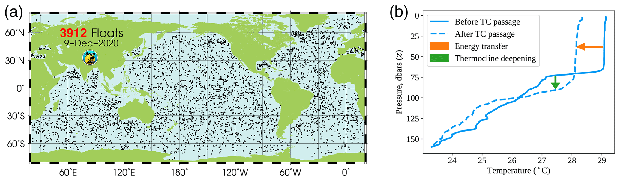
Figure 1(a) Argo floats have achieved global coverage since 2007 (Argo Program, 2020). (b) Two consecutive temperature profiles from the same Argo float near Puerto Rico in 2017: one before and one after the passage of Hurricane Maria. The orange arrow depicts the net removal of thermal energy from the ocean, while the green arrow illustrates the deepening of the thermocline as a result of increased mixing.
For our purposes, the chief contribution of Argo to our oceanographic and meteorological pursuits is its provision of vertical information, from the surface of the ocean to roughly 2000 m below the surface, in tandem with its global coverage, with one float per 3° longitude by 3° latitude box on average (Jayne et al., 2017). The vertical information from the Argo profiles, unattainable by remote sensing methods such as satellites, is key to quantifying the thermal response of the ocean to the passage of a TC, which varies with depth. Argo profiles, however, are not without shortcomings for our purposes; their spatiotemporal resolution is coarser than typical TC spatial scales and timescales, which necessitates the statistical methods developed herein.
An Argo float takes a profile in the following fashion. Every sampling period, typically every 10 d, the float descends from its “parking” depth of 1000 m to a profiling depth of 2000 m and then ascends from 2000 m to the surface over the course of about 6 h, taking observations of temperature and salinity along the way (Jayne et al., 2017). It then rests at the surface for 15 min to 1 h, determining its location and communicating its measurements via satellite. Finally, the float returns to its parking depth until its next sampling period to minimize float drift.
In this study, we refer to an individual Argo device as a “float” and to the measurements taken vertically at a certain longitude, latitude, and time as a “profile”. Each Argo profile is uniquely identified by its float identifier (unique to an Argo float) and cycle number (for a given float, unique to each profile).
3.3 TC-centric coordinate system
To quantify the ocean thermal response to the passage of a TC, we perform a pairing procedure inspired by Cheng et al. (2015). Intuitively, we seek pairs of profiles which “straddle” the passage of TC, i.e., one observation before and one observation during or after the TC passage. These Argo profile pairs are placed in a TC-centric coordinate system through a projection process, which rewrites the space–time coordinates of an Argo profile pair in reference to a passing tropical cyclone. Figure 2 illustrates this process using the TC track and profile pairs associated with Hurricane Maria (2017), and the full set of profile pairs in the TC-centric coordinate system is depicted in Fig. 3b. The pairing and projection procedures are formalized in Sect. 4.2.
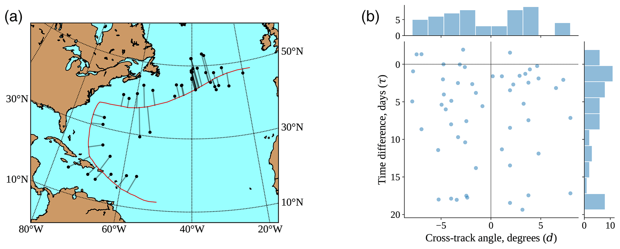
Figure 2Illustration of the coordinate systems with Hurricane Maria (2017). Panel (a) uses the latitude–longitude coordinate system to show the path of the storm in red and the location of the Argo profile pairs straddling the storm passage in black. Panel (b) plots those same pairs of profiles in the TC-centric coordinate system. It is possible for one black point in the latitude–longitude coordinate system to correspond to multiple observations in the TC-centric coordinate system, if a single profile occurring before TC passage is paired with multiple profiles occurring after TC passage.
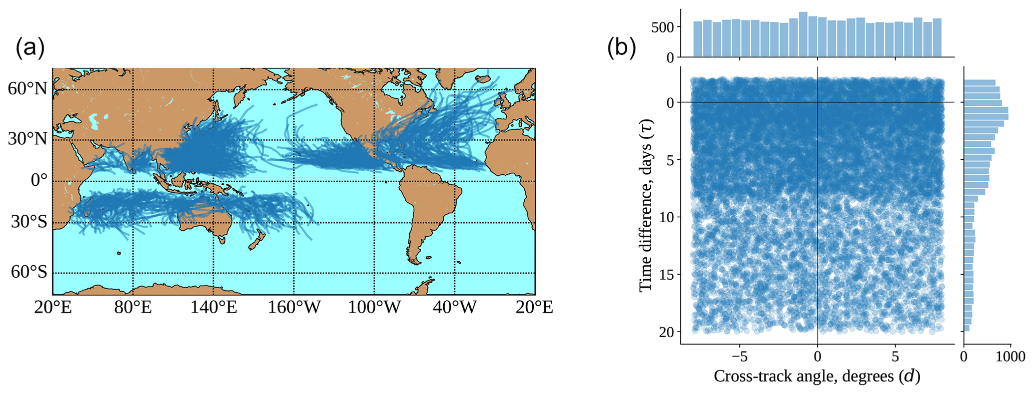
Figure 3(a) Global tropical cyclones from 2007 to 2018 in the latitude–longitude coordinate system, for 1089 tracks in total. (b) Argo profile pairs in the TC-centric coordinate system, for 16 025 pairs in total. Marginal histograms illustrate the density of the pairs along the time and cross-track axes.
The methodology introduced in this paper aims to produce a representation of the TC-induced change in ocean temperature, at a sequence of fixed depths and as a continuous function of time since the tropical cyclone passage and cross-track distance from the center of the tropical cyclone path. To properly characterize these temperature changes, we combine a variety of techniques for pairing Argo profiles, estimating seasonal effects, modeling space–time covariances, and smoothing in multiple dimensions.
All notations will be formally introduced in their requisite subsections, but in general x refers to a location in the latitude–longitude coordinate system, t refers to the day of the year, d refers to the cross-track angle between a location and the center of the storm path, and τ refers to the time difference between a post-storm Argo profile and the passage of the tropical cyclone with which is it associated, measured in days.
Before the detailed exposition, we provide a high-level explanation of our modeling approach, which will be further formalized as an ANOVA decomposition data model. First, we partition the Argo profile database into “TC profiles”, which report time stamps immediately before and after the passage of a TC, and “non-TC profiles”, which are bounded away from TCs in space and time (Sect. 4.1.2). Using the TC profiles, we form in Sect. 4.2 pairs of Argo profiles, in which the two profiles “straddle” the passage of a TC; i.e., one profile occurs before (the “baseline” profile) and one profile occurs during or after the TC passage (the “signal” profile). Then, we decompose the observed temperature difference (at each pressure level) between the baseline and signal profiles in the following manner.
The nonrandom seasonal effect term is estimated in Sect. 4.3 and is subtracted from the temperature differences to produce seasonally adjusted temperature differences. The ocean variability (noise) term is then estimated in Sect. 4.4; it is the only term on the right-hand side regarded as random. These two terms describe the state of the ocean under the assumption that there are no TC-induced effects; therefore, partitioning of Argo profiles into TC and non-TC profiles in Sect. 4.1.2 is crucial to their estimation, as the latter observe the ocean in the TC-absent regime.
The key subject of interest is the TC signal term, which we denote by s(d,τ) to emphasize its dependence on the cross-track distance from the storm center and the time since storm passage. Our goal is to make inferences for functionals H(s) of s. This includes point evaluators, e.g., , as in Sect. 5.2, and binned quantities, e.g., , as in Sect. 5.4.
To elucidate the estimation of s(d,τ), we describe each of the terms in Eq. (1) formally, in terms of an ANOVA decomposition. Let T denote an Argo temperature observation, evaluated at a fixed pressure level z. The temperature difference is the difference between the two terms Tsignal−Tbaseline:
where m is a seasonal mean field and a is a Gaussian process term describing non-TC ocean variability, both elucidated fully in Sect. 4.3 and 4.4.
A few remarks are in order. First, note that Tsignal is written as a function of both Earth's coordinates and TC-centric coordinates (d,τ), which are uniquely determined by Earth's coordinates and the associated TC path. This is no accident: while m and a are estimated and only have meaning in terms of Earth's coordinates, s is estimated and only has meaning in terms of TC-centric coordinates. Second, we observe that, in theory, Eq. (3) suggests that one may directly estimate s(d,τ) using only observations of Tsignal (and the non-TC profile set). Unfortunately, one finds that the magnitude of a is such that estimating s solely using Tsignal is difficult, due to a low signal-to-noise ratio. By taking the temperature difference Tsignal−Tbaseline, we take advantage of the high correlation between and to yield results with a considerably better signal-to-noise ratio.
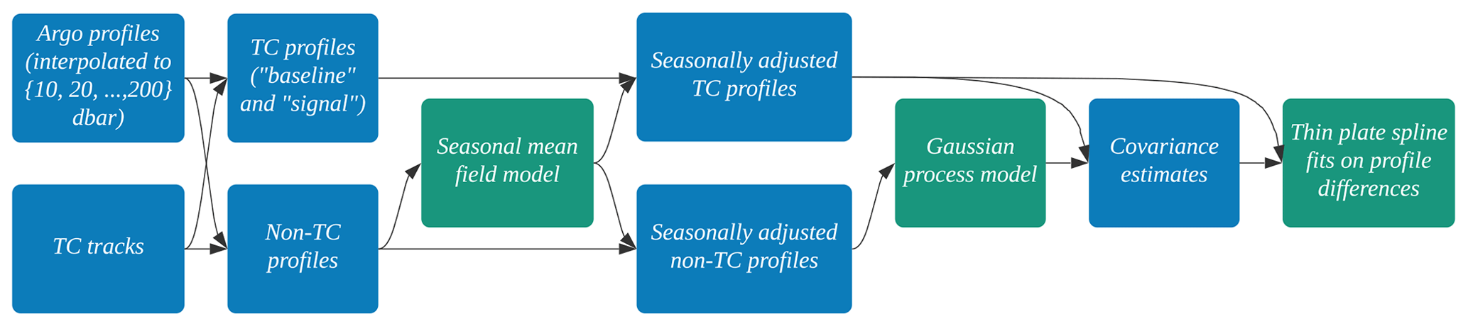
Figure 4Illustration of the multi-step framework as a data analysis pipeline. The data and results are denoted in blue, and the statistical models are denoted in green.
The partitioning of the Argo profile database into TC and non-TC profile sets is described in Sect. 4.1.2. The pairing process and the construction of the observed temperature difference are detailed in Sect. 4.2. Section 4.3 explains the estimation of the seasonal effect based upon spatiotemporal local regression modeling, and Sect. 4.4 describes a space–time Gaussian process model for the remaining ocean variability term. Finally, Sect. 4.5 leverages thin-plate splines to produce a final fit of the TC signal s(d,τ). We depict the full framework as a data analysis pipeline in Fig. 4.
4.1 Argo profile preprocessing
In this section, we describe two key preprocessing steps performed on the Argo profiles.
4.1.1 Interpolation and averaging
An unprocessed Argo temperature profile consists of a sequence of {(zi,Ti)} which relates pressure level zi to temperature measurements Ti. We take each Argo temperature profile and interpolate them from a pressure level of z=10 dbar to z=200 dbar using a piecewise cubic Hermite interpolating polynomial (pchip interpolant; Fritsch and Carlson, 1980). We then read off 20 equally spaced values from z=10 dbar to z=200 dbar, including the endpoints. We also compute the average temperature by performing a trapezoidal integration of the pchip over a grid of 5000 evaluations, normalized by the length of integration (190 dbar). We refer to the former as the gridded temperature values and to the latter as the vertically averaged temperature values.
In the analysis that follows, we use the term Argo profile to refer to the collection of the 20 gridded temperature values and the vertically averaged temperature value. The partitioning, pairing, and projection procedures of Sect. 4.1.2 and 4.2 operate on these collections of values on the profile level. The statistical methodology, developed in Sect. 4.3, 4.4, and 4.5, considers each of the gridded pressure levels (and the vertically averaged temperature values) separately; i.e., the statistical analysis is performed 21 times, for each of and for the averaged temperatures.
We use T to denote a single temperature value, either the evaluation of the pchip interpolant at a pressure level z or the vertically averaged value. As the methodology is identical for each pressure level and for the vertically averaged profiles, we do not burden T with additional notation; which of the gridded and vertically averaged temperature values it is will be made clear from the context.
4.1.2 TC profiles and non-TC profiles
We further partition the Argo profile database into two sets, which separately characterize the ocean state in the presence and absence of TCs. If an Argo profile is within 8° (latitude and longitude) of a tropical cyclone observation location and within 12 d before to 20 d after that tropical cyclone observation, we denote it as a tropical cyclone profile (TC profile). Any profile not in this set is denoted as a non-tropical cyclone profile (non-TC profile). Though the non-TC profiles do not carry any of the TC signal s(d,τ), they play a crucial role in estimating the seasonal effect m and ocean variability a, which characterize the ocean state and dynamics under the important assumption that there are no TC-related effects. These models are fully described in Sect. 4.3 and 4.4.
4.2 Profile–TC association process
To associate Argo profiles with tropical cyclones, we perform a two-step procedure of pairing and projection. In the pairing step, we identify Argo profiles that are close to each other and straddle a passing tropical cyclone such that one profile is observed before the storm to characterize the pre-storm ocean state (referred to as the baseline profile), and another is observed during or after the storm to characterize the change in the ocean state (referred to as the signal profile). In the projection step, we change the coordinate system of the Argo profile pairs to one parameterized in terms of the passing tropical cyclone. This is done by performing an orthogonal projection of the Argo profile pair onto the tropical cyclone track. Both procedures are formalized in the sequel.
We first establish notation. Define the Earth coordinates as , i.e., the longitude, latitude, and time that the baseline and signal profiles were taken, and the TC-centric coordinates as (d,τ), where d is the signed great circle angular distance on Earth between (xlon,xlat) and π(xlon,xlat), the orthogonal projection onto the tropical cyclone track, and τ is the time difference between tsignal and , the time when the tropical cyclone was at π(xlon,xlat). Due to the closeness constraints that we impose between the baseline and signal profiles, described in the following subsection, only one set of longitude–latitude coordinates is necessary for both profiles.
4.2.1 Pairing process
We follow closely the pairing process introduced in Cheng et al. (2015). Recall that the tropical cyclone tracks are available at 6-hourly time resolution and can be made continuous in time and space through straight line interpolation. Along each of these TC tracks, we seek Argo profiles that reported within ±8° (longitude–latitude) and within 12 d before to 20 d after each location on the tropical cyclone track. We partition these profiles into the baseline set (−12 to −2 d relative to the TC) and the signal set (−2 to +20 d relative to the TC). These two sets contain the profiles that are incidental to the TC. The baseline and signal time ranges are chosen primarily to accommodate sampling constraints posed by the Argo network; specifically, most floats sample on a 10 d frequency. Therefore, the baseline time range of −12 to −2 d ensures that each float can contribute at least one baseline profile. The signal time range allows for at least two signal profiles from a given float (assuming they fit a nearness condition detailed in the sequel). The signal profiles begin at −2 d to hedge against storm effects prior to passage and are consistent with the pairing process introduced by Cheng et al. (2015).
Among profiles incidental to a given TC, we perform a pairing process as follows. If there exist a profile in the baseline set and a profile in the signal set that are at most 0.2° apart2, we pair them, yielding a baseline profile and signal profile pair. Under this closeness restriction, we make the simplifying assumption that the baseline and signal locations are spatially identical, and for each pair we use the baseline location as the reference point. We defer a discussion of how to potentially extend our model to account for Argo float movement and rigorously incorporate intra-pair spatial differences to Sect. 6.
We impose an additional technical restriction with respect to the lineage of a baseline profile, which is defined as the set of all signal profiles associated with a distinct baseline profile and that baseline profile itself. We require that all profiles in the lineage of a baseline profile must be separated in time by at least 72 h, sparsifying the lineage. To our knowledge, Cheng et al. (2015) impose no such constraint. The choice of this separation is for a particular reason: we know that pairs of profiles close in time tend to be highly correlated, but our Gaussian process model (Kuusela and Stein, 2018) for estimating the correlations between pairs of profiles that are close in space and time (a prerequisite for properly handling them in the final thin-plate spline fit) may not provide reliable estimates in the rare cases where profiles occur more frequently than 3 d apart. Following a filter on the minimum time separation within each lineage, we retain 16 025 profile pairs across all five ocean regions: 2757 in the North Atlantic, 2897 in the eastern Pacific, 778 in the Indian Ocean, 2185 in the Southern Hemisphere, and 7409 in the western Pacific.
4.2.2 Projection process
Given these Argo profile pairs, which we know straddle a TC path, we require a procedure for precisely describing the profile pair's location in space and time relative to the passage of the tropical cyclone. Recall that we formally denote the location of the Argo profile pair by and that there is no distinction between the baseline and signal locations, as we assume they are the same. Through our pairing procedure, we rewrite the coordinates of the Argo profile pair with respect to a nearby tropical cyclone in terms of .
The projection procedure proceeds as follows. Each tropical cyclone track is made continuous through straight line interpolation. We project each profile pair from (xlon,xlat) to π(xlon,xlat), the nearest point on the tropical cyclone track in the Euclidean sense. Given π(xlon,xlat), we obtain , the time at which the tropical cyclone was at π(xlon,xlat), using linear interpolation. Finally, we obtain the cross-track angle
and the time since passage
where is the induced angle between two points on Earth's surface with respect to its center, and the subtraction in Eq. (5) is performed in a “year-aware” fashion; i.e., if the year–day difference is negative, as may happen over the new year, then we add the number of days in the year prior to the difference. The projection process is depicted in Fig. 2, using profile pairs associated with Hurricane Maria (2017) as an example.
4.3 Seasonal mean field estimation
Although the temperature differences induced by tropical cyclone passage occur on relatively small temporal scales, there is a nontrivial seasonal effect experienced by the ocean during the tropical cyclone season, at the timescales considered in our analysis. We focus here on the methodology for estimating the seasonal cycle and fully detail the resulting empirical findings in Sect. 5. In order to properly account for the seasonal effect, we adapt previous methodology (Ridgway et al., 2002; Roemmich and Gilson, 2009) to estimate a global mean field specifically for the “counterfactual”; i.e., we characterize the state of ocean temperatures during the TC season, using the non-TC profiles of Sect. 4.1.2.
Using the non-TC profiles of Sect. 4.1.2, we estimate, separately for each pressure level and for the vertically averaged temperature values, a global mean field through a variant of the Roemmich–Gilson climatology. The Roemmich–Gilson climatology (Roemmich and Gilson, 2009) was among the first to take advantage of the spatial coverage of the Argo array to characterize the mean state and annual cycle of temperature in the global upper ocean. Specifically, they used a local linear regression model (Ridgway et al., 2002) to estimate the climatological mean temperature as a function of location (xlon,xlat), pressure level z, and day of year t. This model is written down explicitly in Kuusela and Stein (2018), and our model, which differs marginally from that of Roemmich and Gilson (2009) in that we do not weight observations based upon the distance from the center point or use data from pressure levels to form estimates at pressure level z, is elucidated in Eq. (6).
At each of these 20 pressure levels (or for the vertical average) and at each grid point of a mesh consisting of 180 equally spaced latitude points and 360 equally spaced longitude points, we fit
to the temperature observations, using all the non-TC profiles that fall within ±8° (longitude–latitude) of the point at which our local regression function is centered. Since these models are fit separately over each window and depth, the estimation procedure can be trivially parallelized.
Let us denote by the mean function derived by fitting a local linear regression with data within a window centered at using Eq. (6) for a fixed depth z or for the vertically averaged temperature values. Then, for each of the TC profiles (Sect. 4.1.2), we produce the seasonal mean-adjusted temperature value in the following fashion. For a profile located at at time t with temperature value T, obtain the closest grid point at which a local linear function was fitted:
Then, at each pressure level , we obtain the mean-adjusted profiles:
For each temperature value T in the TC profile set, we apply this mean adjustment to obtain the seasonally adjusted temperature value . In particular, for a baseline–signal temperature pair Tbaseline,Tsignal, occurring at times tbaseline,tsignal, we obtain the seasonally adjusted temperature value pair . This gives rise to the seasonally adjusted temperature differences
In terms of the high-level model Eq. (1), Eq. (9) in fact represents the temperature difference without the seasonal effect. This may be seen through the decomposition:
since the last two mean field terms only differ in terms of the contribution of the seasonal harmonics in Eq. (6).
Having accounted for the non-stochastic seasonal term, we may now directly analyze the reduced model. This is informally described as
and formally described, in terms of the ANOVA decomposition, as
where we have economized the notation from Eqs. (2) and (3) for brevity. The fitted seasonal means, at a depth of z=40, are depicted in Fig. 5, with the full set of estimates across all pressure levels deferred to the Supplement. The practical effect of this seasonal adjustment is illustrated in Sect. 5.1. The mean field adjustment is also performed for the non-TC profiles, yielding mean zero observations for the purposes of fitting the Gaussian process model of Sect. 4.4.
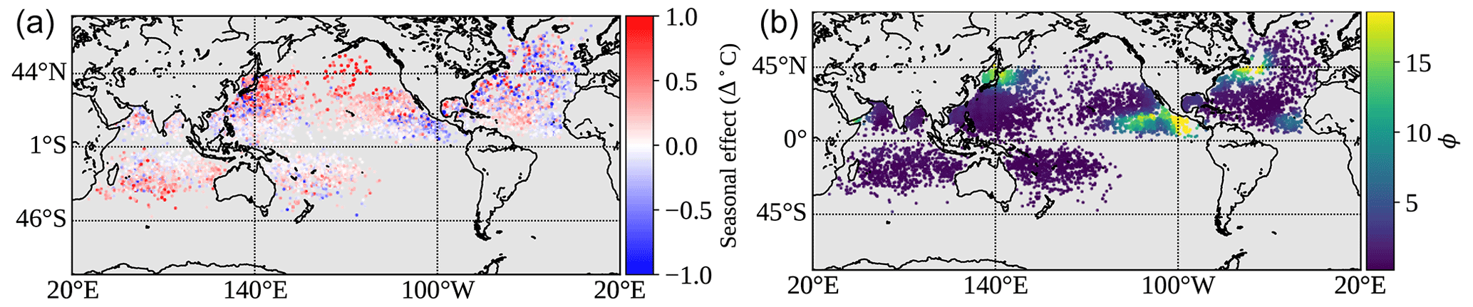
Figure 5Panel (a) displays the seasonal effects fitted to the baseline–signal profile pairs, which show a general warming pattern during the TC season. Because these seasonal effects are for pooled profile pairs from various times during the tropical cyclone season, the fitted effects may appear “noisy” as a function of latitude and longitude; as a function of ambient space and time, the mean fields are smooth, as expected for the local regression model (6). Panel (b) displays the ϕ parameters, which are the dominant term of the ocean variability estimates. These fitted parameters reveal higher noise in regions corresponding to the equatorial currents off Central America, the Kuroshio and Oyashio currents off Japan, and the Gulf Stream current off Nova Scotia (Talley, 2011). Estimates at TC profile locations and pressure level z=40 are displayed here, though the underlying model fits are performed on a global grid. The full set of estimates across all pressure levels is deferred to the Supplement.
4.4 Variability estimates
Having obtained seasonally adjusted temperature differences at all pressure levels, we next detail our method for estimating the variability of these temperature differences. Our general approach is an adaptation of the Gaussian process model proposed by Kuusela and Stein (2018), which handles the globally nonstationary covariance structure of the ocean using locally stationary Gaussian processes in a moving-window fashion (Haas, 1990, 1995). As in Sect. 4.3, we learn the parameters of our model using the non-TC profiles, in order to capture the local dynamics of the ocean without TC-induced effects. However, once fitted, the model is used to provide information about ocean variability in the time and locations of the TC profiles. This is a subtle, but important, distinction.
Our local Gaussian process models are fitted on an equally spaced grid of 180 latitude points and 360 longitude points, with a time window centered on September. This prioritizes fidelity towards ocean dynamics during the late summer and early fall months, when tropical cyclones are prevalent in the Northern Hemisphere, where the majority of the TC profile pairs are observed. As before, this analysis is carried out separately at each pressure level and for the vertically averaged temperature values.
In the following exposition, we follow the notation of Kuusela and Stein (2018), with slight adaptations to maintain consistency with Sect. 4.3. We use the term mean-adjusted interchangeably with seasonally adjusted to emphasize that the mean-adjusted temperature values are zero-mean (in the absence of a TC signal), as required by the Gaussian process model assumptions.
Let denote a mean-adjusted temperature value associated with a non-TC Argo profile at a fixed pressure level. At each grid point and fixed pressure level z, we assume the following model for data points falling spatially within a window of ±5° of the grid point and temporally within the 3 months centered on September:
where indexes the years and indexes the observations within the geospatial window for each year, xi,j is the spatial location associated with the mean-adjusted temperature value , and ti,j is the time at which it was observed. The εi,j is a Gaussian nugget effect (Cressie, 1993), with , and denotes a zero-mean Gaussian process with a stationary covariance function with parameters . The specific function used is an anisotropic geospatial covariance function
with ϕ>0, where
with . As in Kuusela and Stein (2018), these parameters are obtained through the method of maximum likelihood. As with the local mean field, the estimation of these parameters may be done in parallel across windows and pressure levels.
A few remarks are in order. First, we note that the fitted parameters ϕ(x), θlat(x), θlon(x), θt(x), σ(x) are all functions of , as we assume local stationarity to capture global nonstationarity. At each location, the Gaussian process model used to estimate these parameters is centered on September, as most TCs in our database occur during this time period. We then use these parameters to model the variance structure of profile pairs in all ocean basins; one could refine these estimates by fitting a model centered about every month and using the model whose central month is closest in time to each profile pair. Finally, we observe that, by construction, the profile pairs from Sect. 4.2 are assumed to have the same locations, i.e., and . Therefore, the covariance between the two profiles in a profile pair is given by the following reduced expressions. For a mean-adjusted temperature value pair located at (xlon,xlat) with times tbaseline,tsignal, let be the nearest grid point, as in Sect. 4.3, and let as in Eq. (12) be
To give an impression of the general variability in the global ocean, we plot the fitted ϕ parameters, for a fixed pressure level z=40, in Fig. 5. The parameters ϕ are plotted because ϕ is the dominant term in each variability estimate. The full set of figures depicting the fitted parameters and temperature difference variances, at each pressure level, is deferred to Sect. S5 of the Supplement.
We note that, even though only ϕ, θt, and σ are used to evaluate the data covariances, the full model (Eqs. 12, 13, and 14) must be fitted to estimate these parameters, and we require the full Argo database, including the non-TC profiles, to obtain these estimates.
For simplicity, we assume that two profiles which do not share the same baseline profile are uncorrelated. However, there are cases in which the lineage of a baseline profile includes multiple signal profiles. In these cases, we account for the covariance between the profiles in the lineage. We detail the case in which there are two signal profiles with mean-adjusted temperature values , associated with a baseline profile with a mean-adjusted temperature value , but the following framework is trivially extended to an arbitrary number of signal profiles in the lineage. In practice, there will be no more than six signal profiles for a given baseline profile, due to the separation constraint introduced in Sect. 4.2. Define the shorthand . We suppress the location x′ at which the parameters are evaluated, for brevity. First, consider the covariance structure between the mean-adjusted temperature values of the three profiles in this lineage (one baseline and two signal values, occurring at times ):
The covariance matrix for the temperature differences may then be obtained as follows. Define the mean-adjusted temperature differences
and the shorthand . Observe that y(ijk) is simply a linear transformation of :
In general, the transformation matrix is a column of minus ones horizontally concatenated with the identity matrix. It immediately follows that
Recall that, because the temperature differences have been mean-adjusted, they are assumed to be zero-mean in the absence of a TC signal. Therefore, when there is no TC signal, the distribution of y(ijk) is Gaussian with mean zero and covariance cov(y(ijk)), given in Eq. (21). Mathematically speaking, we have accounted for the variability term of Eq. (11). This forms the basis for the estimation of s(d,τ), our key quantity of interest, in Sect. 4.5.
4.4.1 Computational remarks
Denote by y the full set of mean-adjusted temperature differences, ordered such that profiles in the same lineage are contiguous. Its covariance, cov(y), is a block diagonal matrix, with dense blocks corresponding to the lineages of distinct baseline profiles. This is important for two reasons. First, a block diagonal matrix admits an efficient inverse; i.e., the inverse of a block diagonal matrix may be obtained by inverting the blocks individually. Each of these blocks is no more than six entries wide, due to the separation constraint placed on profiles in Sect. 4.2. Second, the sparse structure of the block diagonal matrix may be exploited for efficient linear algebra operations (Virtanen et al., 2020) necessary to construct the thin-plate splines described in the sequel.
4.5 Thin-plate splines
Having learned a model for the term of Eq. (11) through the Gaussian process model of Sect. 4.4, we find ourselves properly positioned to estimate the TC-induced signal s(d,τ). This we do with a thin-plate spline, a flexible nonparametric technique for fitting a surface in two dimensions, subject to a curvature penalty and observation weights. Specifically, we smooth the seasonally adjusted temperature differences using a fixed-knot thin-plate spline smoother (Duchon, 1977; Wahba, 1980, 1990; Green and Silverman, 1994; Nychka, 2000; Wood, 2017), in which we use the covariances estimated in Sect. 4.4 to account for heteroskedasticity and cross-observation dependence (Rao, 1973; Draper and Smith, 1998; Nychka, 2000; Ruppert et al., 2003). As with the local mean field model of Sect. 4.3 and the Gaussian process model of Sect. 4.4, this procedure is conducted separately at each pressure level and for the vertically averaged profiles.
We use a fixed-knot smoother (rather than placing a knot at every design point), chiefly in order to improve the conditioning of the linear operators. As an additional, computational consideration, the use of fixed knots reduces the time and space complexity of the procedure. The fixed knots are equally spaced in the domain, in a grid formed from the cross-product of 33 points on the cross-track axis and 45 points on the time axis. This yields a knot every 0.5 units along each dimension, including on the boundary.
The weighting of observations by the covariance between temperature differences is also noteworthy. From a data model standpoint, it is known that we are using observations with drastically different noise levels , , due to the effect of time and location. Since we have estimated these noise levels in Sect. 4.4, the covariance reweighting allows us to directly incorporate this information when estimating s(d,τ) into the reduced model Eq. (11). From a practical standpoint, the covariance reweighting has a real effect in improving the signal-to-noise ratio, as shown in Fig. 7 of Sect. 5.2. The full details of the thin-plate spline smoother, including its motivation and derivation, are given in Appendix A.
Let be the design points and be the corresponding responses. We further fix a grid of regularly spaced knots, , m≪n, on which the basis functions of our smoother will be centered. We use the shorthand notation , , and . Finally, we denote by a weight matrix. Traditionally, this is the inverse covariance matrix of the observations y.
In our usage, we take to be the (d,τ) coordinates of our Argo profile pairs, as obtained from Sect. 4.2; to be the corresponding seasonally adjusted temperature differences y of those pairs, as obtained from Sect. 4.3; and to be the inverse matrix of covariances between those seasonally adjusted temperature differences, as obtained from Sect. 4.4. Therefore, here , where the first dimension (cross-track angle) is measured in degrees and the second dimension (time since TC passage) is measured in days.
The fixed-knot covariance-reweighted thin-plate spline problem is posed as follows. We seek coefficients δ,β such that the following objective is minimized:
The first term in Eq. (22) is a generalized least-squares (Rao, 1973; Draper and Smith, 1998; Ruppert et al., 2003) data-fit criterion, and the second term is a roughness penalty (Meinguet, 1979; Green and Silverman, 1994; Wood, 2017), with defined in the sequel. The parameter λ>0 mediates the competing demands of the data fidelity and roughness penalty terms.
4.5.1 Construction of the smoother
The fixed-knot thin-plate spline smoother with covariance reweighting is constructed as follows. Denote by the radial basis matrix with entries:
Note that this consists of radial basis functions centered on the knots , evaluated at the data points ξi. Further denote by the basis matrix corresponding to the linear and constant terms:
Finally, we define an additional “basis” matrix, where we evaluate the radial basis functions at the knot locations :
for the purpose of evaluating the roughness penalty in Eq. (22).
The coefficients minimizing Eq. (22) are given (see Appendix A) by
where are the coefficients corresponding to the radial basis functions centered at the fixed knots and are the coefficients corresponding to the constant and linear terms. Estimates of the signal s(d,τ) at a new set of locations may be obtained as follows:
where we denote with entries
and
4.5.2 Uncertainty quantification
Estimate variances and confidence intervals follow for the thin-plate spline estimates through the linearity of the smoother and the assumption of Gaussian noise. Denote by the observation covariance matrix cov(y) from Eq. (21). The covariance matrix of the estimates is given by
where
The form of Eq. (30) follows from the usual quadratic form of covariances.
The matrix can be exorbitantly large (e.g., in our use case, we produce estimates on a grid with locations). However, the construction of pointwise confidence intervals (i.e., , appealing to the Gaussian assumption to obtain 95 % coverage) only requires evaluation of the diagonal entries of , allowing for significant computational savings. We note that, although the derived confidence intervals have widths matching the standard deviation of the estimates, the estimates themselves are biased due to shrinkage; therefore, the confidence intervals technically have biased centers. It is thus possible that the intervals are misplaced, or are too short, in regions where s(d,τ) experiences high curvature. We discuss alternatives for improvement in Sect. 6.
5.1 Seasonal mean field adjustment
First, we detail the effect of the seasonal mean field adjustment, described in Sect. 4.3, on the observed data. Recall that the model (6) is fitted separately at each pressure level . In Fig. 6, we depict the effect of the seasonal adjustment on temperature differences at a pressure level of z=40 dbar. The raw temperature differences are displayed in Fig. 6a, with the seasonal differences plotted in Fig. 6b and the seasonally adjusted temperature differences in Fig. 6c. The latter is the result of subtracting (b) from (a). The individual differences are subject to an isotropic Gaussian kernel smoother with a bandwidth of σ=0.2, in order to more clearly display the data.
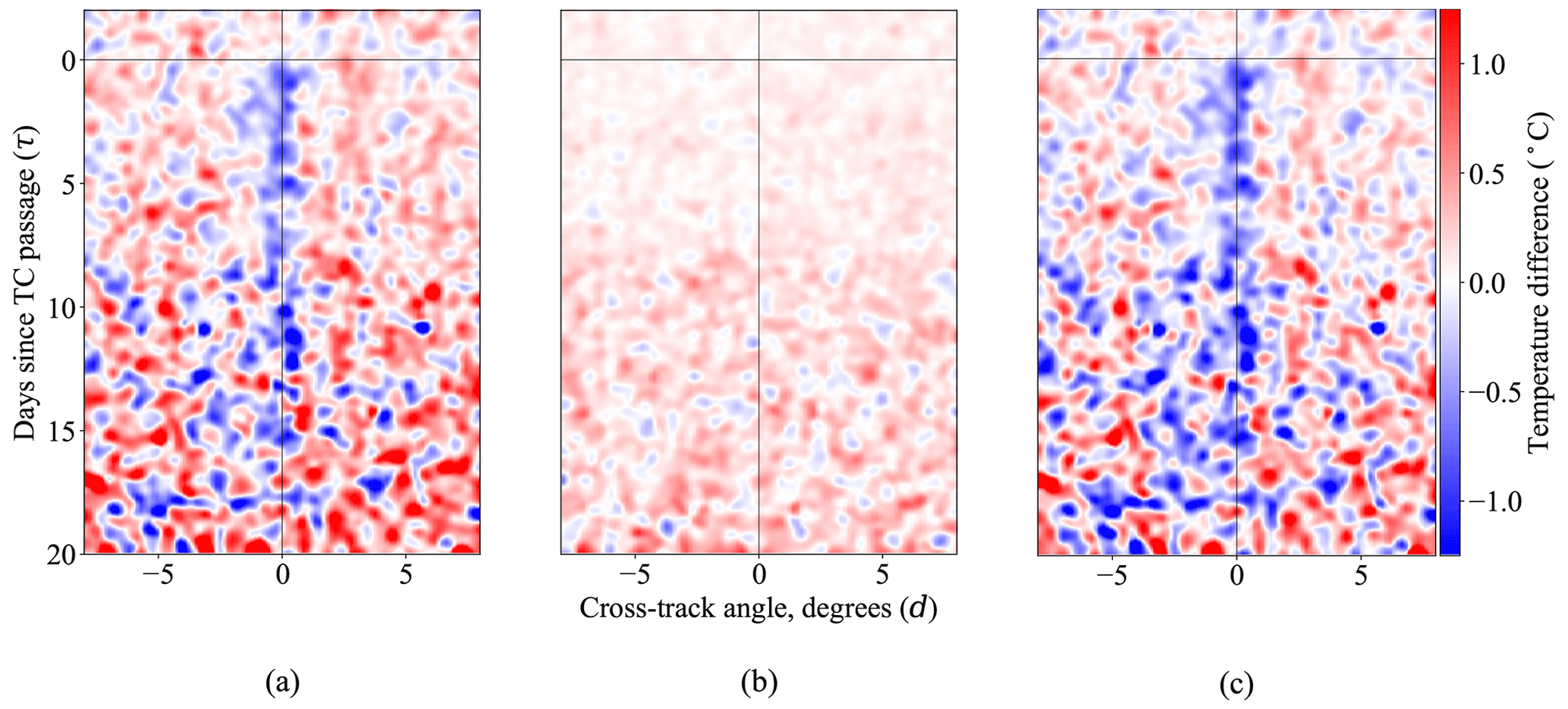
Figure 6Temperature differences in the (d,τ) coordinate system, at a depth of 40 m. Panel (a) depicts the raw temperature differences, panel (b) shows the fitted mean field, and panel (c) shows the seasonally adjusted temperature differences. Here we include all profile pairs across all storm intensities and subject the data to a local constant smoother with an isotropic Gaussian kernel of bandwidth σ=0.2.
Figure 6b shows a warming effect that increases in magnitude as the time between the signal profile and TC passage increases. This is consistent with the notion that the ocean experiences an overall warming effect at this depth during the TC season. Note that because we are plotting the difference in the mean field evaluated at the times and locations of actual TC-associated profile pairs, we are only examining the mean field differences during the tropical cyclone season of each ocean basin analyzed. Similar to Fig. 5, here the fitted seasonal effects are pooled over the entire TC season (and from different locations on Earth), which makes the fitted differences appear “noisy” in the TC-centric coordinate system, but the fitted mean fields are smooth as a function of ambient space and time, as expected based upon Eq. (6).
The warming effect in the seasonal mean field difference is a consistent feature in the pressure levels z=30 through z=150. The pressure levels do not show a warming pattern and might even exhibit a slight cooling effect, while the pressure levels z≥160 show only a small contribution of the seasonal signal to differences in paired profiles. These phenomena are consistent with the spatial structure of the seasonal cycle (Roemmich and Gilson, 2009). An adjustment for seasonal warming was not performed in a previous analysis of the ocean thermal response using paired Argo profiles (Cheng et al., 2015); as a result, some of the warming effects previously observed over longer time spans may in fact have been due to seasonal variation. The full sequence of results at all 20 pressure levels is deferred to Sect. S1 of the Supplement.
5.2 Ocean thermal response as a continuous function of time and cross-track distance
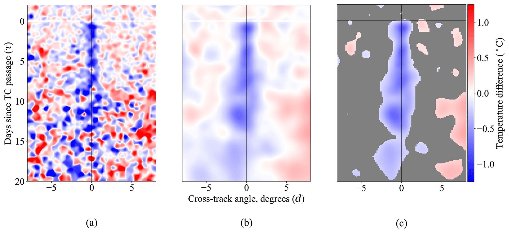
Having adjusted the temperature differences for the seasonal change using the model detailed in Sect. 4.3 and accounted for the variability across profile pairs via Sect. 4.4, we now apply the thin-plate spline smoother to the seasonally adjusted temperature differences to obtain our main scientific result: a characterization of the ocean thermal response to the passage of hurricane-strength tropical cyclones as a continuous function of time and cross-track distance. This function is depicted for data from profile pairs associated with a hurricane-strength tropical cyclone (formally defined as having a sustained wind speed of at least 64 kn at , the time of TC passage) at a pressure level of z=10 dbar in Fig. 7.
The thin-plate splines are fitted separately at each depth z. Within each , we select a tuning parameter guided by leave-one-out cross-validation (LOOCV). Importantly, we do not take the that directly minimizes the LOOCV score. Instead, we take the that produces a LOOCV error slightly (1 %) larger than the minimum LOOCV error. This is done because heterogeneity in the thermal response signal causes a direct minimization of the LOOCV score to oversmooth the signal. The full details of the cross-validation procedure, including its mathematical statement, plots illustrating the estimated test error achieved by different λ, and the chosen , are deferred to Appendix B.
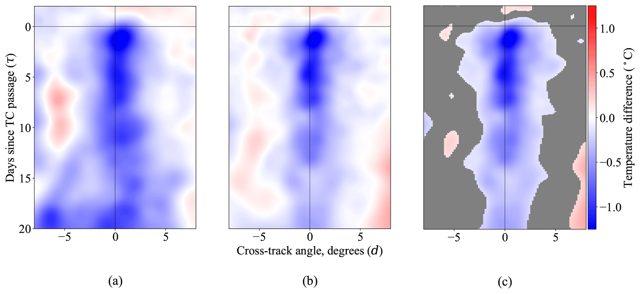
Figure 7Temperature differences for hurricane-strength profile pairs in the (d,τ) coordinate system, at a depth of 10 m, smoothed using thin-plate splines. Panel (a) depicts a thin-plate spline fit without any variance reweighting, panel (b) shows a thin-plate spline fit using block covariance reweighting, and panel (c) shows a pointwise α=0.5 test. We observe in panel (a) an unusual positive anomaly at cross-track , time difference , as well as unusually strong negative differences at time difference . Reweighting by the estimated block covariance in panel (b) attenuates these anomalies, and a pointwise hypothesis test in panel (c) masks these phenomena, indicating that they were due to ocean variability noise unrelated to TCs.
The central Fig. 7b depicts the thin-plate spline fit, accounting for correlation between observations at a depth of z=10 dbar. Formally, the correlation adjustment is performed as follows. We obtain an estimate for Σ=cov(y) through the Gaussian process model of Sect. 4.4 and provide this to our covariance-reweighted thin-plate spline smoother of Sect. 4.5 by setting . Recall that, by construction, Σ is a block diagonal matrix, with blocks no larger than six entries wide; therefore, Σ−1 may be efficiently computed. For a very small number of temperature differences, the fitted variance is extremely small, on the order of . We truncate the left tail and filter out these observations to prevent distortion of the fit. This omits only 488 observation pairs out of 16 025.
In Fig. 7c, we perform a pointwise level α=0.05 hypothesis test on the thin-plate spline fit, using the variance estimates derived in Sect. 4.5. The issues of performing a pointwise hypothesis test with N=40 000 points are manifold, and we defer discussion of extensions through which we could make the significance test more sophisticated to Sect. 6. Nonetheless, we see in Fig. 7c a simple fact: that the estimated cooling effect induced by tropical cyclones is of a greater magnitude than the variability of the estimates. Moreover, this cooling effect persists for a sustained period of time, stretching into 2 weeks following the tropical cyclone passage. We also see a rightward bias in the cooling effect, which may be attributed to the storm's direction of rotation.3
To illustrate the importance of estimating the correlations between observations for the final thin-plate spline fit, we plot in Fig. 7a the surface estimated by applying a thin-plate spline smoother without accounting for the variability estimates from Sect. 4.4, i.e., setting W to be the identity matrix. These estimates are tuned with the same LOOCV procedure. We observe a sustained warm anomaly at that is present over several days. Concerningly, this warm anomaly is comparable in magnitude with the expected cooling effect observed at d≈0. We also see negative anomalies which occur late in the recovery stage, in . When viewed in context with Fig. 7b and c, we see that adjusting for the correlations reduces the impact of some outlying observations causing these anomalous effects in the naive estimate, and the pointwise hypothesis test masks away the effects almost entirely.
An additional phenomenon of scientific interest that may be observed in the thin-plate spline fits is that of vertical mixing, in which the warm water close to the ocean surface is forced downwards by the force of the tropical cyclone (Mei and Pasquero, 2013). Although the net change in heat content incidental to the passage of a tropical cyclone is negative, vertical mixing may register as a warming effect at shallower subsurface ocean depths. This phenomenon may be observed in Fig. 8. In Fig. 8a, we recall the smoothed temperature differences at depth z=10, in which a dramatic cooling effect is depicted. At the deeper pressure level of z=60, however, we see a mixture of both cooling and warming; i.e., a net increase in temperature is observed at , . Finally, we see in Fig. 8c that, by z=150, the warming effect has disappeared, while the cooling effect remains. We note that the characterization of this warming effect as a continuous function of both cross-track angle and time since TC passage is made possible by our methodological framework and was not possible in the previous literature (Cheng et al., 2015).
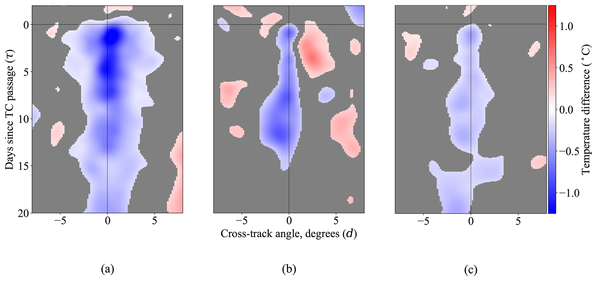
Figure 8Temperature differences for hurricane-strength profile pairs, smoothed using thin-plate splines, at depths of , and 150, respectively. Vertical mixing gives rise to a warming phenomenon on the right side of the tropical cyclone at the intermediate depths. All plots are masked with a pointwise level α=0.05 hypothesis test.
The discussion of vertical mixing is further developed in Sect. 5.3, 5.4, and 5.5. The full set of covariance-reweighted thin-plate spline fits, at all pressure levels , is deferred to Sect. S2 of the Supplement.
5.3 Depth–time parameterization
Of additional scientific interest is the characterization of the ocean thermal response for a fixed cross-track angle, as a function of time and pressure. To facilitate this analysis, we collect the 20 thin-plate spline fits for pressure levels from Sect. 5.2 and “marginalize” them along three sets of cross-track angles: , , and . These three plots are presented in Fig. 9. In each of the marginalized plots, we subset the covariance-reweighted thin-plate spline fits from Sect. 5.2 to each of the cross-track bins and average out the cross-track component. Variance estimates follow immediately (owing to the linearity of averaging) and are used to construct a pointwise α=0.05 hypothesis test. We display these marginalized estimates in Fig. 9.
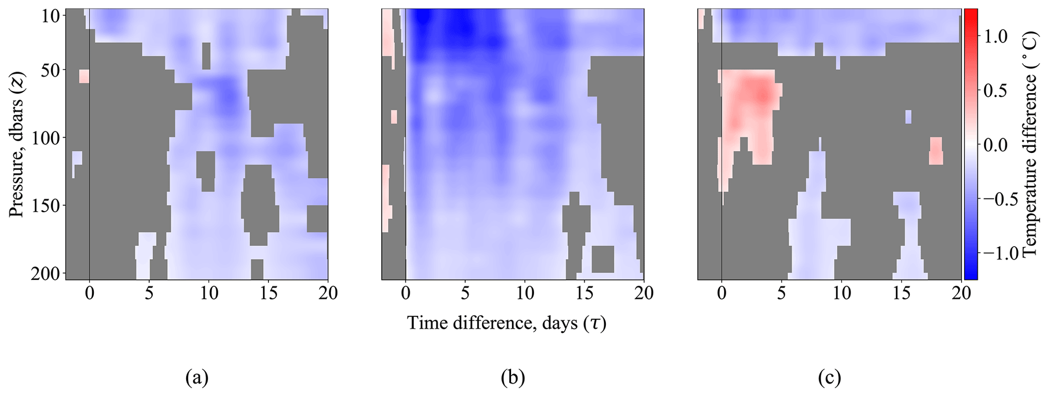
Figure 9The covariance-reweighted thin-plate spline fits (hurricane-strength TCs) of Sect. 5.2 are averaged along three sets of cross-track angles d corresponding to the left (), center (), and right () relative to the TC's forward movement. The resulting estimates are plotted as a function of time since TC passage τ and pressure level z. A pointwise α=0.05 hypothesis test is performed and used to mask areas where we fail to reject the null hypothesis.
The cross-track angle bins, centered on , were chosen to emphasize three particular oceanographic and meteorological phenomena. First, the bin centered on d=0 in Fig. 9b depicts the ocean cooling induced by the passage of tropical cyclones. Of particular note is the fact that this cooling appears to persist for a sustained period of time, specifically up to at least 2 weeks. As one may expect, the cooling effect diminishes as pressure z or time since TC passage τ increases. Second, the bin centered at in Fig. 9c depicts the phenomenon of vertical mixing previously discussed in Sect. 5.2. As TC winds mix surface water downward, we observe warming at depths between z=50 and z=150. Past z=150, we find that the warming effect has faded away. Finally, we contrast the strong warming effect observed in Fig. 9c with the lack of warming (at a statistically significant level) in Fig. 9a, which depicts the bin centered on . This reflects the fact that the effect of vertical mixing is asymmetric, due to the counterclockwise rotation of tropical cyclones in the Northern Hemisphere.
5.4 Depth–cross-track parameterization
We further demonstrate that our continuous-time methodology captures the temporally binned results of Cheng et al. (2015), whose profile pairing process we used in this paper. To introduce temporal binning, we take the covariance-reweighted thin-plate spline estimates from Sect. 5.2 across pressure levels and split them into two bins, and , termed the “forced” stage and “recovery” stage by Cheng et al. (2015). For each of the two bins, we perform the same averaging process as in Sect. 5.3 to marginalize the estimates over the τ axis and obtain α=0.05 pointwise significance tests. We present the resulting fits as functions of cross-track angle d and pressure level z in Fig. 10.
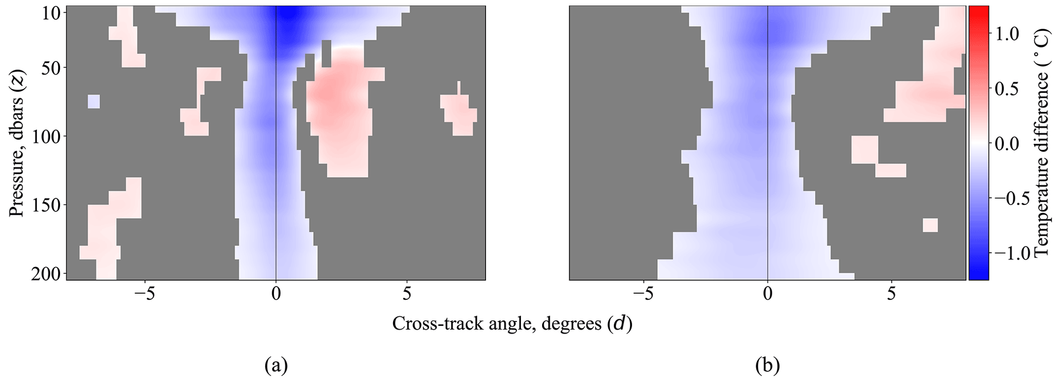
Figure 10The covariance-reweighted thin-plate spline fits (hurricane-strength TCs) of Sect. 5.2 are averaged along two sets of time since TC passage τ, and the resulting estimates are plotted as a function of pressure level z and cross-track angle d. Panel a averages over d, and panel b averages over d. A pointwise α=0.05 hypothesis test is performed and used to mask areas where we fail to reject the null hypothesis.
Several noteworthy phenomena are present in Fig. 10. In Fig. 10a, we observe both the primary cooling effect and the secondary warming effect in the subsurface on the right side of the storm due to vertical mixing, as discussed in Sect. 5.2 and 5.3. We also observe a sustained cooling effect in Fig. 10b during the period called the “recovery” stage in Cheng et al. (2015). While the primary cooling effect observed in the two time periods is qualitatively consistent with the results presented by Cheng et al. (2015), their results also show a strong warming effect on both sides of the storm during the recovery stage (Fig. 10 in Cheng et al., 2015), which is absent from our estimate. Overall, it appears that the recovery stage estimate in Cheng et al. (2015) is “warm biased” in comparison to our estimate. We attribute the difference to our methodology's accounting of the seasonal mean field and variability estimates, which, when used in the thin-plate spline estimate, attenuate the influence of outlying observations dominated by non-TC oceanographic variability as illustrated in Fig. 7.
5.5 Isosurfaces of the thin-plate spline estimates
To provide a holistic understanding of the ocean thermal response structure as a function of depth, cross-track distance, and time since TC passage, we compute isosurface plots of the thin-plate spline estimates from Sect. 4.5. Two sets of isosurfaces are computed: one set for regions of negative temperature differences and one set for regions of positive temperature differences. These are shaded blue and red, respectively, in Fig. 11.
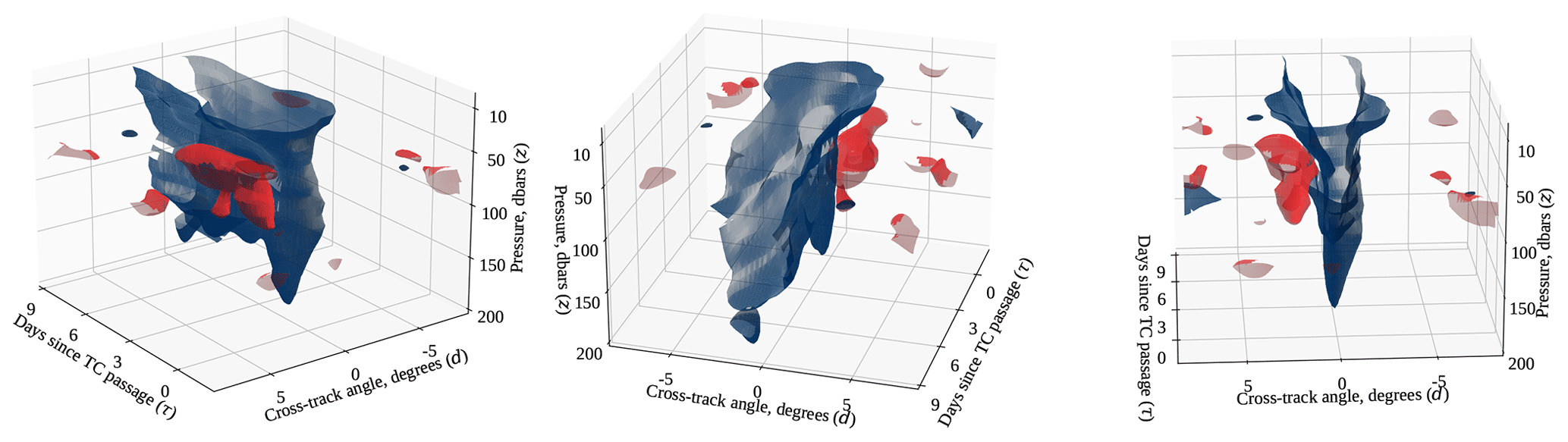
Figure 11The ±0.3 °C isosurfaces of the thin-plate spline fits, displayed at three different camera perspectives. Negative temperature differences are shaded in blue, and positive temperature differences are shaded in red.
For each set of isosurfaces, we first mask the thin-plate spline estimates that fail to reject a pointwise level α=0.05 hypothesis test, using the variance estimates from Sect. 4.5.2. We then apply the marching cubes algorithm (Lorensen and Cline, 1987; Lewiner et al., 2012; Virtanen et al., 2020) to identify positive and negative isosurfaces of magnitude 0.3 °C. The positive isosurface is colored in red and the negative isosurface in blue.
We observe in Fig. 11 a large blue mass corresponding to the TC-related ocean cooling. This blue mass is restricted to a relatively small range of cross-track angles near the center but persists in time. This behavior is consistent with Fig. 9. We also observe a smaller red mass, corresponding to the local warming effect associated with the vertical mixing induced by the TC, as previously seen in Fig. 8 and discussed in Sect. 5.3. Consistent with Figs. 8, 9, and 10, this warming effect is only observed on the positive side of the cross-track distance axis. The right panel of Fig. 11 mirrors Fig. 10a almost exactly, the only differences being the viewing angle and filtering of very small values inherent in finding nonzero isosurfaces.
5.6 Vertically averaged temperature differences
Here, we present the results from the vertically averaged analysis, in which we estimate the full model Eqs. (2) and (3) using the vertically averaged temperature values from Sect. 4.1.1. As before, we choose the smoothing parameter guided by leave-one-out cross-validation, with the full details deferred to Appendix B.
The seasonally adjusted temperature differences and accompanying thin-plate spline fits are presented in Fig. 12. In Fig. 12a, we only show data from pairs associated with hurricane-strength TCs, in contrast to Fig. 6, which shows data from all profile pairs regardless of storm intensity. The restriction to hurricane-strength profile pairs here is to provide a fairer comparison with the thin-plate spline estimates of Fig. 12b and c, which use the hurricane-strength subset (as in Fig. 7).
The thin-plate spline fit in Fig. 12b conforms to our intuition; we observe a cooling signal, as in Fig. 7b, but its magnitude is dampened by the vertical averaging procedure. More importantly, Fig. 12c does not show any warming effect indicative of vertical mixing. This is in contrast to Figs. 7b, 9c, and 10a, which treat depth as a separate dimension of analysis. From an oceanographic and meteorological perspective, this suggests that the vertical mixing-induced warming effect is local in depth; it only appears at some pressure levels, because it is caused by the forcing of warm surface waters downward by the TC. Once we integrate vertically, the local warming effect is cancelled out by a cooling effect near the surface and is no longer visible. From a statistical perspective, this underscores the importance of treating depth as a separate axis of analysis, using the vertical resolution of Argo observations.
In this paper, we have introduced a comprehensive methodological framework based upon an ANOVA-type decomposition for analyzing tropical-cyclone-induced ocean temperature changes. This framework includes a pairing process for identifying reference observations, the construction of an annual mean field to account for seasonal shift at the timescales of the measured differences, and estimation of observation variability and computationally efficient smoothers that leverage these estimates of variability.
Aside from methodological contributions, we have presented several results of scientific interest. In particular, our framework improves upon the past scientific literature by modeling the tropical-cyclone-induced ocean thermal response as a function of time, pressure, and cross-track angle, in which both the time and cross-track angle components are treated continuously. Through this modeling, we are able to produce fine-grained characterizations of the ocean thermal response at a number of different depths, and we observe differing ocean thermal responses as a function of depth. Specifically, we recover the primary effect of surface cooling and the secondary effect of subsurface warming due to vertical mixing. By computing isosurfaces on our thin-plate spline fits, we are able to characterize these two phenomena as a function of the depth, time, and cross-track distance dimensions. Finally, the seasonal mean field component of our methodological framework reveals a nontrivial warming of the ocean near its surface during the TC season, which we estimate and account for in our analysis.
Of course, this is not the full scientific story. The ocean response to the passage of TCs is complex, including contributions from upwelling near the storm center, downwelling in the outer regions, and mixed-layer entrainment (Elsberry et al., 1976; Lin et al., 2017); horizontal currents (D'Asaro et al., 2007); and air–sea exchanges of heat (Emanuel, 1986, 1999). The initial stratification in a region is also important for understanding the relevant processes. Nonetheless, the statistical methodology presented in this paper provides an important new framework through which TC-induced temperature changes in the upper ocean may be studied as a function of depth, distance from the TC track center, and time since TC passage.
Although our methodological framework was developed with ocean thermal response in mind, the techniques discussed are of general interest. An immediate generalization is the use of the exact same methodology for Argo salinity profiles in lieu of temperature profiles. One may expect that, due to rainfall, evaporation, and mixing, the passage of a tropical cyclone would be registered in the salinity profiles of the affected ocean region. Similar analyses for other transient atmospheric phenomena, including atmospheric rivers and southern ocean storm systems, are also possible. One could additionally regress these signals on latitude, storm strength, pre-storm ocean state, ocean basin, and other covariates to better model and understand the underlying scientific phenomena. Regression on latitude may be particularly relevant with regard to the ongoing scientific discourse on the large-scale climatological effects of tropical cyclones (Emanuel, 2001; Korty et al., 2008; Jansen and Ferrari, 2009; Jansen et al., 2010; Haney et al., 2012).
The present methodological framework also admits a number of possible refinements. From a statistical standpoint, one could improve upon our model by considering each temperature profile to be a functional observation and modeling the depth component continuously rather than interpolating to a sequence of depths and fitting separate models at each depth level. This would potentially allow one to also infer changes in mixed-layer depth and thermocline stability. Our model could also potentially be improved by replacing the thin-plate spline smoother with a spline smoother with a spatially varying smoothing parameter (e.g., Ruppert and Carroll, 2000) or a nonlinear, multiresolution smoother that naturally accounts for heterogeneity in the TC-induced signal (e.g., Daubechies et al., 1999).
The pointwise hypothesis tests used in Sect. 5.2 have a number of limitations, including a lack of correction for multiple testing and smoothing bias. These provide natural opportunities for improvement; however, the problem of amending the pointwise hypothesis tests could be subsumed by instead considering field significance (e.g., Livezey and Chen, 1982; Wilks, 2006; DelSole and Yang, 2011). Because the primary goal of this paper is to introduce a general methodological framework of which the final hypothesis tests are just one component, we defer these improvements to future work.
An additional extension of statistical and scientific interest involves carefully accounting for float drift. In this paper, we require the baseline and signal profiles to be within 0.2° of each other and then assume that they share a single location in the analysis, admitting a useful simplification of the fitted covariance function. An extension would involve relaxing the strict closeness requirement of the paired profiles and removing the assumption that the paired profiles are in the same location by more carefully modeling their covariance, taking into account their relative spatial locations. This requires a nontrivial generalization of the Gaussian process model of Kuusela and Stein (2018) but would provide the benefit of increasing the number of available pairs with which to fit the model. An early approach in this vein is that of Paciorek and Schervish (2006). Yet another extension would be the consideration of parametric models for the TC wake (Haney et al., 2012). Finally, the fusion of microwave sea surface temperature (mSST; Gentemann et al., 2003; Wentz et al., 2005) observations with Argo profiles might provide an opportunity to produce estimates of the individual-storm level rather than in terms of the global aggregates, as was done here. mSST observations are very dense in latitude and longitude but lack the depth penetration provided by the Argo profiles, which are relatively sparse in latitude and longitude. Therefore, mSST and Argo are naturally complementary in the information provided.
In this section, provided for completeness, we motivate and derive the thin-plate spline estimator (Duchon, 1977; Wahba, 1980, 1990; Green and Silverman, 1994; Wood, 2003) used in Sect. 4.5 for completeness. First, we review the natural thin-plate spline smoother in Sect. A1. Sections A2 and A3 then describe versions of the thin-plate spline when subject to covariance reweighting (via generalized least squares; Rao, 1973; Draper and Smith, 1998; Nychka, 2000; Ruppert et al., 2003) and when its basis functions are constructed from a fixed-knot set (Wahba, 1980; Wood, 2017).
A1 The natural thin-plate spline smoother
Suppose we observe data with responses . Define the shorthand notation and .
The natural thin-plate spline problem provides a smooth function g such that g(ξi)≈yi for . The “closeness” of g(ξi) to yi is enforced through squared error, while a penalty on the curvature of g discourages roughness. Formally, we define the roughness penalty:
We then define an objective in which the regularization parameter λ>0 mediates the competing demands of the squared error and roughness penalty terms:
Let us define the basis matrix , with entries
One may recognize this as analogous to the basis matrix Eq. (23) from Sect. 4.5, where we have replaced the fixed knots with a knot at each sample point. Further recall the basis of linear and constant terms in Eq. (24).
It is possible (Duchon, 1977; Meinguet, 1979; Wahba, 1980, 1990; Green and Silverman, 1994) to rewrite Eq. (A2) as
where uniquely define the thin-plate spline g. Expanding Eq. (A4), we obtain
Therefore, first-order optimality and convexity imply that Eq. (A3) is minimized by such that
A2 The covariance-reweighted thin-plate spline smoother
Due to the correlated and heteroskedastic nature of the temperature differences in this paper, we desire a version of the thin-plate spline smoother Eq. (A6) that properly accounts for these effects. This is done via generalized least squares (Rao, 1973; Draper and Smith, 1998; Nychka, 2000; Ruppert et al., 2003), which poses the objective function
where is the inverse of the covariance matrix between the seasonally adjusted temperature differences, previously estimated in Sect. 4.4. In the simplest case of diagonal W, Eq. (A7) may be interpreted as inversely weighting the contribution of each observation to the objective by the magnitude of its variance.
Carrying through an analogous quadratic expansion and minimization, we find that Eq. (A7) is minimized by such that
A3 Adaptation to fixed knots
Finally, we detail the adaptation of the covariance-reweighted thin-plate spline smoother to the fixed-knot regime (Wahba, 1980, 1990; Ruppert et al., 2003; Wood, 2017). Suppose a set of fixed knots , with as defined in Eq. (23) and S as defined in Eq. (25). The thin-plate spline smoothing problem, restricted to this set of knots, is given (Wood, 2017) by
where δ∈ℝm and β∈ℝ3. Carrying out the same calculations, we find that Eq. (A9) is minimized by such that
In this section, we fully describe the procedure used to select the in Sect. 5.2 and the in Sect. 5.6. Informally, we calculate the leave-one-out cross-validation (LOOCV) scores for a fine grid of λ and then choose the λ corresponding to the most complex model whose LOOCV score is within 1 % of the minimum LOOCV. This procedure is motivated by the fact that the signal being estimated is heterogeneous, and a naive minimization of the LOOCV error was empirically found to result in an over-regularized model. This will be made formal in the sequel.
The leave-one-out cross-validation score under weighted smoothing (Cook and Weisberg, 1982; Green and Silverman, 1994) is given by
where wi is an observation-specific weight (typically the inverse variance) and is the thin-plate spline, fitted to all observations except observation i, using regularization parameter λ, evaluated on observation i.
As the thin-plate spline is a linear smoother, we may trivially access the leave-one-out residuals through the “hat matrix trick” (Cook and Weisberg, 1982; Green and Silverman, 1994)
where is the ith diagonal entry of the hat matrix of , i.e., the matrix H(λ) that satisfies . Combining Eqs. (B1) and (B2), we obtain the LOOCV score
where we have taken , as in Sect. 4.5.
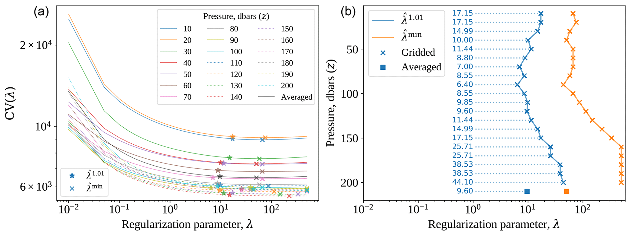
Figure B1Panel (a) shows that the minimizing , for each depth, tends to lie in an extremely shallow basin, within which a wide range of λ achieves a comparable estimated test error (NB: the vertical axis is at the logarithmic scale). By choosing a associated with a 1 % increase in the test error, we obtain fits that more faithfully illustrate the TC-induced thermal response. Panel (b) reports the chosen for each pressure level z and for the vertically averaged temperature differences. Fits using λ>500 are ignored as they essentially only fit the linear (unpenalized) terms of the thin-plate spline.
The LOOCV errors for fits and for the vertically averaged fit are illustrated in Fig. B1, with the minimizing marked with crosses in Fig. B1a. However, as we alluded to earlier, we do not use ; rather, we take
which we mark with stars in Fig. B1a. This corresponds to taking the most complex model whose LOOCV error is within 1 % of the minimized LOOCV error. We favor a more complex model than the one obtained by naively minimizing the LOOCV error because the signal being estimated is heterogeneous; i.e., it obeys different levels of smoothness in different regions of the domain. The and are given as a function of depth in Fig. B1b.
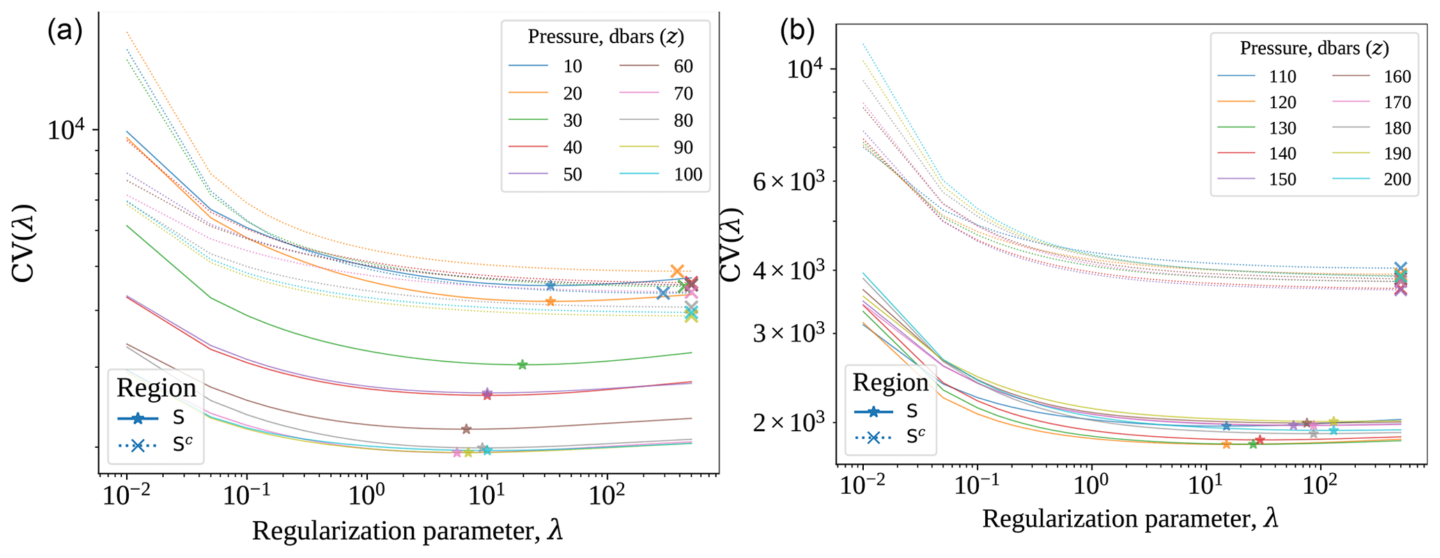
Figure B2LOOCV curves, computed separately using errors within a “thermal response signal” region 𝒮 and errors within 𝒮c. The observations within 𝒮 consistently favor a more complex model; the fact that no single λ is uniformly optimal over the entire domain highlights the heterogeneity of the signal being estimated. We compromise by allowing a more complex model that achieves an LOOCV error within 1 % of the minimum.
Specifically, the signal is particularly large in magnitude for cross-track angles (d) close to zero and within the first 2 weeks after TC passage (τ); however, outside of this region, the signal drops off and is close to zero in curvature. For illustrative purposes, we formally define this “thermal response signal” region as . We then compute two LOOCV error curves for each depth z, one using data from 𝒮 and the other using data from .
Indeed, we see in Fig. B2 that the LOOCV curves implied by the errors corresponding to observations in each of these two regions produce very different minimizers, with the observations within the thermal response signal region favoring a more complex model and observations outside the signal region favoring a more regularized model. The choice of represents a compromise between the natural impulse to minimize the LOOCV error and the recognition that naive minimization will yield an over-regularized model, as was empirically confirmed to be the case when visually inspecting the fits. Importantly, the , tuned using only the observations falling in 𝒮, are roughly consistent with our slightly under-smoothed , as can be seen by comparing Figs. B1 and B2.
Code implementing our methodology may be found at https://github.com/huisaddison/tc-ocean-methods (last access: 30 December 2022) and Zenodo (https://doi.org/10.5281/zenodo.11882987, Hu, 2022).
There are two principal sources of data: Argo float data and tropical cyclone best-track data. The Argo float data were collected and made freely available by the International Argo Program and the national programs that contribute to it (https://doi.org/10.17882/42182, Argo, 2000). The Argo Program is part of the Global Ocean Observing System. The tropical cyclone best-track data are available from the National Hurricane Center (2022) website (https://www.nhc.noaa.gov/data/#hurdat).
The supplement related to this article is available online at: https://doi.org/10.5194/ascmo-10-69-2024-supplement.
AJH, MK, and ABL developed the methodology with domain knowledge and conceptualization from DG and KMW. AJH performed the formal analysis, visualization, and writing, with feedback from all the authors. The software was developed by AJH, extending the original software by MK.
The contact author has declared that none of the authors has any competing interests.
Publisher’s note: Copernicus Publications remains neutral with regard to jurisdictional claims made in the text, published maps, institutional affiliations, or any other geographical representation in this paper. While Copernicus Publications makes every effort to include appropriate place names, the final responsibility lies with the authors.
We thank the associate editor and the two referees, whose feedback improved the quality and clarity of our paper. The authors thank members of the CMU Statistical Methods for the Physical Sciences (STAMPS) Research Group and the SAMSI/CMU Statistical Oceanography Working Group for insightful comments and feedback during this work.
Addison J. Hu acknowledges support from the NSF GRFP (award no. DGE175016) and NSF DMS (award no. 1520786). Mikael Kuusela was supported by the NOAA (award no. NA21OAR4310258). Ann B. Lee was supported by the NSF DMS (award no. 2053804). Donata Giglio was supported by NSF EarthCube (award no. 1928305), the NOAA (award no. NA21OAR4310261), and NASA (award no. 80NSSC19K0059). Kimberly M. Wood was supported by the NSF (award no. AGS-2011812).
This paper was edited by Christopher Paciorek and reviewed by two anonymous referees.
Argo: Argo float data and metadata from Global Data Assembly Centre (Argo GDAC), SEANOE [data set], https://doi.org/10.17882/42182, 2000. a
Argo Program: Implementation status, https://argo.ucsd.edu/about/status/ (last access: 10 December 2020), 2020. a
Balaguru, K., Chang, P., Saravanan, R., Leung, L. R., Xu, Z., Li, M., and Hsieh, J.-S.: Ocean barrier layers' effect on tropical cyclone intensification, P. Natl. Acad. Sci. USA, 109, 14343–14347, https://doi.org/10.1073/pnas.1201364109, 2012. a
Balaguru, K., Foltz, G. R., Leung, L. R., Asaro, E. D., Emanuel, K. A., Liu, H., and Zedler, S. E.: Dynamic Potential Intensity: An improved representation of the ocean's impact on tropical cyclones, Geophys. Res. Lett., 42, 6739–6746, https://doi.org/10.1002/2015GL064822, 2015. a
Bender, M. A. and Ginis, I.: Real-Case Simulations of Hurricane–Ocean Interaction Using A High-Resolution Coupled Model: Effects on Hurricane Intensity, Mon. Weather Rev., 128, 917–946, https://doi.org/10.1175/1520-0493(2000)128<0917:RCSOHO>2.0.CO;2, 2000. a, b, c
Cheng, L., Zhu, J., and Sriver, R. L.: Global representation of tropical cyclone-induced short-term ocean thermal changes using Argo data, Ocean Sci., 11, 719–741, https://doi.org/10.5194/os-11-719-2015, 2015. a, b, c, d, e, f, g, h, i, j, k, l, m, n, o, p, q, r
Chu, J.-H., Sampson, C. R., Levine, A. S., and Fukada, E.: The Joint Typhoon Warning Center Tropical Cyclone Best-Tracks, 1945–2000, Tech. Rep. NRL/MR/7540-02-16, Joint Typhoon Warning Center, https://www.metoc.navy.mil/jtwc/products/best-tracks/tc-bt-report.html (last access: 10 December 2020), 2002. a
Cione, J. J. and Uhlhorn, E. W.: Sea Surface Temperature Variability in Hurricanes: Implications with Respect to Intensity Change, Mon. Weather Rev., 131, 1783–1796, https://doi.org/10.1175//2562.1, 2003. a
Cook, R. D. and Weisberg, S.: Residuals and influence in regression, Monographs on statistics and applied probability, Chapman and Hall, New York, ISBN 978-0412242809, 1982. a, b
Cressie, N. A. C.: Statistics for Spatial Data, Wiley Series in Probability and Statistics, John Wiley & Sons, Inc., ISBN 9781119115182, 1993. a
Dare, R. A. and McBride, J. L.: Sea Surface Temperature Response to Tropical Cyclones, Mon. Weather Rev., 139, 3798–3808, https://doi.org/10.1175/MWR-D-10-05019.1, 2011. a
D'Asaro, E. A., Sanford, T. B., Niiler, P. P., and Terrill, E. J.: Cold wake of Hurricane Frances, Geophys. Res. Lett., 34, L15609, https://doi.org/10.1029/2007GL030160, 2007. a, b, c
Daubechies, I., Guskov, I., Schröder, P., and Sweldens, W.: Wavelets on irregular point sets, Philos. T. Roy. Soc. Lond. Ser.-A, 357, 2397–2413, https://doi.org/10.1098/rsta.1999.0439, 1999. a
DelSole, T. and Yang, X.: Field Significance of Regression Patterns, J. Climate, 24, 5094–5107, https://doi.org/10.1175/2011JCLI4105.1, 2011. a
Draper, N. R. and Smith, H.: Applied regression analysis, Vol. 326, John Wiley & Sons, ISBN 9780471170822, https://doi.org/10.1002/9781118625590, 1998. a, b, c, d
Duchon, J.: Splines minimizing rotation-invariant semi-norms in Sobolev spaces, in: Constructive theory of functions of several variables 85–100, Springer, ISBN 978-3-540-08069-5, https://doi.org/10.1007/BFb0086566, 1977. a, b, c
Elsberry, R. L., Fraim, T. S., and Trapnell, R. N.: A mixed layer model of the oceanic thermal response to hurricanes, J. Geophys. Res., 81, 1153–1162, https://doi.org/10.1029/JC081i006p01153, 1976. a, b
Emanuel, K.: Contribution of tropical cyclones to meridional heat transport by the oceans, J. Geophys. Res.-Atmos., 106, 14771–14781, https://doi.org/10.1029/2000JD900641, 2001. a, b, c
Emanuel, K.: 100 Years of Progress in Tropical Cyclone Research, Meteorol. Monogr., 59, 15.1–15.68, https://doi.org/10.1175/AMSMONOGRAPHS-D-18-0016.1, 2018. a
Emanuel, K. A.: An Air-Sea Interaction Theory for Tropical Cyclones. Part I: Steady-State Maintenance, J. Atmos. Sci., 43, 585–605, https://doi.org/10.1175/1520-0469(1986)043<0585:AASITF>2.0.CO;2, 1986. a, b, c
Emanuel, K. A.: Thermodynamic control of hurricane intensity, Nature, 401, 665–669, https://doi.org/10.1038/44326, 1999. a, b, c
Fisher, E. L.: The Exchange of Energy Between the Sea and the Atmosphere in Relation to Hurricane Behavior, J. Meteorol., 15, 164–171, https://doi.org/10.1175/1520-0469(1958)015<0164:TEOEBT>2.0.CO;2, 1957. a
Fritsch, F. N. and Carlson, R. E.: Monotone Piecewise Cubic Interpolation, SIAM J. Numer. Anal., 17, 238–246, https://doi.org/10.1137/0717021, 1980. a
Gentemann, C. L., Donlon, C. J., Stuart-Menteth, A., and Wentz, F. J.: Diurnal signals in satellite sea surface temperature measurements, Geophys. Res. Lett., 30, 1140, https://doi.org/10.1029/2002GL016291, 2003. a
Green, P. J. and Silverman, B. W.: Nonparametric regression and generalized linear models: a roughness penalty approach, no. 58 in: Monographs on statistics and applied probability, Chapman & Hall, London; New York, 1st Edn., ISBN 9780429161056, https://doi.org/10.1201/b15710, 1994. a, b, c, d, e, f
Haakman, K., Sayol, J.-M., van der Boog, C. G., and Katsman, C. A.: Statistical Characterization of the Observed Cold Wake Induced by North Atlantic Hurricanes, Remote Sens., 11, 2368, https://doi.org/10.3390/rs11202368, 2019. a, b
Haas, T. C.: Lognormal and Moving Window Methods of Estimating Acid Deposition, J. Am. Stat. Assoc., 85, 950–963, https://doi.org/10.1080/01621459.1990.10474966, 1990. a
Haas, T. C.: Local Prediction of a Spatio-Temporal Process with an Application to Wet Sulfate Deposition, J. Am. Stat. Assoc., 90, 1189–1199, https://doi.org/10.1080/01621459.1995.10476625, 1995. a
Haney, S., Bachman, S., Cooper, B., Kupper, S., McCaffrey, K., Van Roekel, L., Stevenson, S., Fox-Kemper, B., and Ferrari, R.: Hurricane wake restratification rates of one-, two- and three-dimensional processes, J. Mar. Res., 70, 824–850, https://doi.org/10.1357/002224012806770937, 2012. a, b, c, d
Hu, A. J.: huisaddison/tc-ocean-methods: v0.0.1 (v0.0.1), Zenodo [code], https://doi.org/10.5281/zenodo.11882987, 2024. a
Jansen, M. and Ferrari, R.: Impact of the latitudinal distribution of tropical cyclones on ocean heat transport, Geophys. Res. Lett., 36, L06604, https://doi.org/10.1029/2008GL036796, 2009. a, b
Jansen, M. F., Ferrari, R., and Mooring, T. A.: Seasonal versus permanent thermocline warming by tropical cyclones: thermacline warming by tropical cyclones, Geophys. Res. Lett., 37, L03602, https://doi.org/10.1029/2009GL041808, 2010. a, b
Jayne, S., Roemmich, D., Zilberman, N., Riser, S., Johnson, K., Johnson, G., and Piotrowicz, S.: The Argo Program: Present and Future, Oceanography, 30, 18–28, https://doi.org/10.5670/oceanog.2017.213, 2017. a, b, c, d, e, f
Joint Typhoon Warning Center: Frequently Asked Questions – Naval Oceanography Portal, https://www.usno.navy.mil/JTWC/frequently-asked-questions-1/frequently-asked-questions (last access: 30 December 2022), 2015. a
Korty, R. L., Emanuel, K. A., and Scott, J. R.: Tropical Cyclone–Induced Upper-Ocean Mixing and Climate: Application to Equable Climates, J. Climate, 21, 638–654, https://doi.org/10.1175/2007JCLI1659.1, 2008. a, b
Kuusela, M. and Stein, M. L.: Locally stationary spatio-temporal interpolation of Argo profiling float data, P. Roy. Soc. A-Math., 474, 20180400, https://doi.org/10.1098/rspa.2018.0400, 2018. a, b, c, d, e, f, g
Landsea, C. W. and Franklin, J. L.: Atlantic Hurricane Database Uncertainty and Presentation of a New Database Format, Mon. Weather Rev., 141, 3576–3592, https://doi.org/10.1175/MWR-D-12-00254.1, 2013. a
Leipper, D. F.: Observed Ocean Conditions and Hurricane Hilda, 1964, J. Atmos. Sci., 24, 182–186, https://doi.org/10.1175/1520-0469(1967)024<0182:OOCAHH>2.0.CO;2, 1966. a
Lewiner, T., Lopes, H., Vieira, A. W., and Tavares, G.: Efficient Implementation of Marching Cubes' Cases with Topological Guarantees, J. Graphics Tools, 8, 1–15, https://doi.org/10.1080/10867651.2003.10487582, 2012. a
Lin, I.-I., Wu, C.-C., Emanuel, K. A., Lee, I.-H., Wu, C.-R., and Pun, I.-F.: The Interaction of Supertyphoon Maemi (2003) with a Warm Ocean Eddy, Mon. Weather Rev., 133, 2635–2649, https://doi.org/10.1175/MWR3005.1, 2005. a
Lin, S., Zhang, W.-Z., Shang, S.-P., and Hong, H.-S.: Ocean response to typhoons in the western North Pacific: Composite results from Argo data, Deep-Sea Res. Pt. I, 123, 62–74, https://doi.org/10.1016/j.dsr.2017.03.007, 2017. a, b
Liu, Z., Xu, J., Zhu, B., Sun, C., and Zhang, L.: The upper ocean response to tropical cyclones in the northwestern Pacific analyzed with Argo data, Chin. J. Oceanol. Limn. 25, 123–131, https://doi.org/10.1007/s00343-007-0123-8, 2007. a
Livezey, R. E. and Chen, W. Y.: Statistical Field Significance and its Determination by Monte Carlo Techniques, Mon, Weather Rev., 111, 46–59, https://doi.org/10.1175/1520-0493(1983)111<0046:SFSAID>2.0.CO;2 1982. a
Lloyd, I. D. and Vecchi, G. A.: Observational Evidence for Oceanic Controls on Hurricane Intensity, J. Climate, 24, 1138–1153, https://doi.org/10.1175/2010JCLI3763.1, 2011. a
Lorensen, W. E. and Cline, H. E.: Marching cubes: A high resolution 3D surface construction algorithm, ACM SIGGRAPH Computer Graphics, 21, 163–169, https://doi.org/10.1145/37402.37422, 1987. a
Luo, Z., Wahba, G., and Johnson, D. R.: Spatial–temporal analysis of temperature using smoothing spline ANOVA, J. Climate, 11, 18–28, 1998. a
Mainelli, M., DeMaria, M., Shay, L. K., and Goni, G.: Application of Oceanic Heat Content Estimation to Operational Forecasting of Recent Atlantic Category 5 Hurricanes, Weather Forecast., 23, 3–16, https://doi.org/10.1175/2007WAF2006111.1, 2008. a, b
McTaggart-Cowan, R., Davies, E. L., Fairman, J. G., Galarneau, T. J., and Schultz, D. M.: Revisiting the 26.5°C Sea Surface Temperature Threshold for Tropical Cyclone Development, B. Am. Meteorol. Soc., 96, 1929–1943, https://doi.org/10.1175/BAMS-D-13-00254.1, 2015. a, b
Mei, W. and Pasquero, C.: Restratification of the Upper Ocean after the Passage of a Tropical Cyclone: A Numerical Study, J. Phys. Oceanogr., 42, 1377–1401, https://doi.org/10.1175/JPO-D-11-0209.1, 2012. a
Mei, W. and Pasquero, C.: Spatial and Temporal Characterization of Sea Surface Temperature Response to Tropical Cyclones, J. Climate, 26, 3745–3765, https://doi.org/10.1175/JCLI-D-12-00125.1, 2013. a, b
Mei, W., Primeau, F., McWilliams, J. C., and Pasquero, C.: Sea surface height evidence for long-term warming effects of tropical cyclones on the ocean, P. Natl. Acad. Sci. USA, 110, 15207–15210, https://doi.org/10.1073/pnas.1306753110, 2013. a, b, c
Meinguet, J.: Multivariate interpolation at arbitrary points made simple, Z. angew. Math. Phys., 30, 292–304, 1979. a, b
National Hurricane Center: HURDAT2 best-track data, https://www.nhc.noaa.gov/data/#hurdat, of last access: 30 December 2022. a
Nychka, D. W.: Spatial-process estimates as smoothers, in: Smoothing and regression: approaches, computation, and application, edited by: Schimek, M. G., Wiley, vol. 329, p. 393, ISBN 9781118150658, https://doi.org/10.1002/9781118150658, 2000. a, b, c, d
Paciorek, C. J. and Schervish, M. J.: Spatial modelling using a new class of nonstationary covariance functions, Environmetrics, 17, 483–506, 2006. a
Park, J. J., Kwon, Y.-O., and Price, J. F.: Argo array observation of ocean heat content changes induced by tropical cyclones in the north Pacific, J. Geophys. Res.-Oceans, 116, C12025, https://doi.org/10.1029/2011JC007165, 2011. a
Pasquero, C. and Emanuel, K.: Tropical Cyclones and Transient Upper-Ocean Warming, J. Climate, 21, 149–162, https://doi.org/10.1175/2007JCLI1550.1, 2008. a
Potter, H., DiMarco, S. F., and Knap, A. H.: Tropical Cyclone Heat Potential and the Rapid Intensification of Hurricane Harvey in the Texas Bight, J. Geophys. Res.-Oceans, 124, 2440–2451, https://doi.org/10.1029/2018JC014776, 2019. a
Price, J. F.: Upper Ocean Response to a Hurricane, J. Phys. Oceanogr., 11, 153–175, https://doi.org/10.1175/1520-0485(1981)011<0153:UORTAH>2.0.CO;2, 1980. a, b
Qu, T., Song, Y. T., and Maes, C.: Sea surface salinity and barrier layer variability in the equatorial Pacific as seen from Aquarius and Argo, J. Geophys. Res.-Oceans, 119, 15–29, https://doi.org/10.1002/2013JC009375, 2014. a
Rao, C. R.: Linear statistical inference and its applications, vol. 2 of Wiley Series in Probability and Statistics, John Wiley & Sons, Inc., ISBN 9780470316436, https://doi.org/10.1002/9780470316436, 1973. a, b, c, d
Ridgway, K. R., Dunn, J. R., and Wilkin, J. L.: Ocean Interpolation by Four-Dimensional Weighted Least Squares–Application to the Waters around Australasia, J. Atmos. Ocean. Tech., 19, 1357–1375, https://doi.org/10.1175/1520-0426(2002)019<1357:OIBFDW>2.0.CO;2, 2002. a, b, c
Riser, S. C., Freeland, H. J., Roemmich, D., Wijffels, S., Troisi, A., Belbéoch, M., Gilbert, D., Xu, J., Pouliquen, S., Thresher, A., Le Traon, P.-Y., Maze, G., Klein, B., Ravichandran, M., Grant, F., Poulain, P.-M., Suga, T., Lim, B., Sterl, A., Sutton, P., Mork, K.-A., Vélez-Belchí, P. J., Ansorge, I., King, B., Turton, J., Baringer, M., and Jayne, S. R.: Fifteen years of ocean observations with the global Argo array, Nat. Clim. Change, 6, 145–153, https://doi.org/10.1038/nclimate2872, 2016. a
Roemmich, D. and Gilson, J.: The 2004–2008 mean and annual cycle of temperature, salinity, and steric height in the global ocean from the Argo Program, Prog. Oceanogr., 82, 81–100, https://doi.org/10.1016/j.pocean.2009.03.004, 2009. a, b, c, d, e, f, g
Ruppert, D. and Carroll, R. J.: Theory & Methods: Spatially-adaptive Penalties for Spline Fitting, Aust. NZ J. Stat., 42, 205–223, 2000. a
Ruppert, D., Wand, M. P., and Carroll, R. J.: Semiparametric regression, Cambridge series in statistical and probabilistic mathematics, Cambridge University Press, Cambridge, New York, ISBN 978-0521785167, 2003. a, b, c, d, e
Russell, B. T., Risser, M. D., Smith, R. L., and Kunkel, K. E.: Investigating the association between late spring Gulf of Mexico sea surface temperatures and U.S. Gulf Coast precipitation extremes with focus on Hurricane Harvey, Environmetrics, 31, https://doi.org/10.1002/env.2595, 2020. a
Shay, L. K.: Air-Sea Interactions in Tropical Cyclones, in: World Scientific Series on Asia-Pacific Weather and Climate, World Scientific, vol. 4, 93–131, https://doi.org/10.1142/9789814293488_0003, 2010. a, b
Shay, L. K. and Goni, G. J.: Effects of a Warm Oceanic Feature on Hurricane Opal, Mon. Weather Rev., 128, 1366–1383, https://doi.org/10.1175/1520-0493(2000)128<1366:EOAWOF>2.0.CO;2, 2000. a
Sriver, R. L., Huber, M., and Nusbaumer, J.: Investigating tropical cyclone-climate feedbacks using the TRMM Microwave Imager and the Quick Scatterometer, Geochem. Geophy. Geosy., 9, Q09V11, https://doi.org/10.1029/2007GC001842, 2008. a
Steffen, J. and Bourassa, M.: Barrier Layer Development Local to Tropical Cyclones based on Argo Float Observations, J. Phys. Oceanogr., 48, 1951–1968, https://doi.org/10.1175/JPO-D-17-0262.1, 2018. a
Sun, L., Yang, Y.-J., Xian, T., Wang, Y., and Fu, Y.-F.: Ocean Responses to Typhoon Namtheun Explored with Argo Floats and Multiplatform Satellites, Atmos.-Ocean, 50, 15–26, https://doi.org/10.1080/07055900.2012.742420, 2012. a
Talley, L. D.: Descriptive Physical Oceanography: An Introduction, Academic Press, ISBN 978-0750645522, 2011. a, b
Trenberth, K. E., Cheng, L., Jacobs, P., Zhang, Y., and Fasullo, J.: Hurricane Harvey Links to Ocean Heat Content and Climate Change Adaptation, Earth's Future, 6, 730–744, https://doi.org/10.1029/2018EF000825, 2018. a, b
Trepanier, J. C.: North Atlantic Hurricane Winds in Warmer than Normal Seas, Atmosphere, 11, 293, https://doi.org/10.3390/atmos11030293, 2020. a
Virtanen, P., Gommers, R., Oliphant, T. E., Haberland, M., Reddy, T., Cournapeau, D., Burovski, E., Peterson, P., Weckesser, W., Bright, J., van der Walt, S. J., Brett, M., Wilson, J., Jarrod Millman, K., Mayorov, N., Nelson, A. R. J., Jones, E., Kern, R., Larson, E., Carey, C., Polat, İ., Feng, Y., Moore, E. W., Vand erPlas, J., Laxalde, D., Perktold, J., Cimrman, R., Henriksen, I., Quintero, E. A., Harris, C. R., Archibald, A. M., Ribeiro, A. H., Pedregosa, F., van Mulbregt, P., and SciPy 1.0 Contributors: SciPy 1.0: Fundamental Algorithms for Scientific Computing in Python, Nat. Methods, 17, 261–272, https://doi.org/10.1038/s41592-019-0686-2, 2020. a, b
Wahba, G.: Spline Bases, Regularization, and Generalized Cross Validation for Solving Approximation Problems with Large Quantities of Noisy Data. Proceedings of the International Conference on Approximation Theory in Honor or George Lorenz, Austin, 8–11 January 1980. a, b, c, d, e
Wahba, G.: Spline models for observational data, CBMS-NSF regional conference series in applied mathematics, SIAM, ISBN 978-0-89871-244-5, https://doi.org/10.1137/1.9781611970128, 1990. a, b, c, d
Wentz, F., Gentemann, C., and Hilburn, K.: Three years of ocean products from AMSR-E: evaluation and applications, in: Proceedings, 2005 IEEE International Geoscience and Remote Sensing Symposium, IGARSS'05, IEEE, Seoul, Korea, vol. 7, 4929–4932, https://doi.org/10.1109/IGARSS.2005.1526780, 2005. a
Wilks, D. S.: On “Field Significance” and the False Discovery Rate, J. Appl. Meteorol. Clim., 45, 1181–1189, https://doi.org/10.1175/JAM2404.1, 2006. a
Wood, S. N.: Thin plate regression splines, J. Roy. Stat. Soc. Ser. B, 65, 95–114, https://doi.org/10.1111/1467-9868.00374, 2003. a
Wood, S. N.: Generalized Additive Models: an introduction with R, CRC press, 2nd Edn., ISBN 9781315370279, https://doi.org/10.1201/9781315370279, 2017. a, b, c, d, e
Wunsch, C.: The past and future ocean circulation from a contemporary perspective, Geophys. Monogr., 173, https://doi.org/10.1029/173GM06, 2007. a
Xu, Z., Sun, Y., Li, T., Zhong, Z., Liu, J., and Ma, C.: Tropical Cyclone Size Change under Ocean Warming and Associated Responses of Tropical Cyclone Destructiveness: Idealized Experiments, J. Meteorol. Res., 34, 163–175, https://doi.org/10.1007/s13351-020-8164-4, 2020. a
Measured in terms of the angular distance to the nearest point on the TC track and alternately referred to as the “cross-track distance” and the “cross-track angle”.
The 0.2° is measured in the induced angle between points on Earth's surface and the center of Earth and is invariant to the location on Earth at which the angle is calculated. This corresponds roughly to a maximum distance of 22 km. For reference, the JTWC considers TCs of radius <0.2° to be “very small” (Joint Typhoon Warning Center, 2015).
Due to the Coriolis effect, TCs in the Northern Hemisphere will induce a greater cooling effect on the right side of the cross-track angle parameterization than on the left side, due to the combined effects of forward movement and counterclockwise wind rotation. TCs in the Southern Hemisphere, which experience clockwise wind rotation, will induce a greater cooling effect on the left side. In order to display this effect in a consistent manner across the hemispheres, we flip the sign of the cross-track angle for TCs in the Southern Hemisphere when producing Figs. 6–12.
- Abstract
- Introduction
- Scientific context
- Data
- Statistical methodology
- Estimated subsurface ocean thermal response to tropical cyclones
- Discussion
- Appendix A: Derivation of the thin-plate spline estimator
- Appendix B: Leave-one-out cross-validation
- Code availability
- Data availability
- Author contributions
- Competing interests
- Disclaimer
- Acknowledgements
- Financial support
- Review statement
- References
- Supplement