A bi-level spatiotemporal clustering approach and its application to drought extraction

We present a novel flexible bi-level spatiotemporal clustering algorithm to extract events based on their intensity and spatiotemporal structures. Our algorithm consists of using (i) a novel space-time k-means clustering to obtain spatiotemporally coherent intensity clusters, and (ii) a density-based spatial clustering of applications with noise (DBSCAN) to spatiotemporally section the intensity clusters into individual events. We discuss the development of the algorithm, the selection, tuning and meaning of the parameters within each step, as well as its validation. Finally, we apply the algorithm to a spatiotemporal drought index, standardized vapor pressure deficit drought index (SVDI), over the continental United States (US) from 1980–2021 and show that it captures historical drought events over the continental United States and their spatiotemporal extents.

1 Introduction

Droughts that are characterized by hot and dry weather conditions have severe social, environmental, and economic effects. For example, during the years 2011 and 2012, droughts in the central United States caused over 30 million dollars in agricultural losses (Smith, 2020). Methodologies that can effectively monitor, detect, and assess drought are important tools in managing risks of drought. To this end, we propose a novel and generalizable bi-level spatiotemporal clustering algorithm that is demonstrated on a numerical drought index to extract and characterized drought events over a 42-year period. For this study, we use a drought index based on vapor pressure deficit (VPD). VPD is a measure of atmospheric demand and a key indicator signaling when water vapor is extracted from soil and vegetation, depleting moisture in the landscape. The standard VPD drought index (SVDI) is based on VPD and was first introduced in Gamelin et al. (2022) to detect flash droughts. Flash droughts are intense but brief droughts characterized by rapid onset, short duration, and rapid recovery. More generally, SVDI has been successful in identifying larger-scale drought patterns and events (Gamelin et al., 2025). By applying the proposed spatiotemporal clustering algorithm to the SVDI index, we present a new and automated approach to extract and understand spatiotemporal clusters of droughts.

The foundational spatial clustering algorithm upon which many other drought extraction approaches are based was first presented in Andreadis et al. (2005). Andreadis et al. (2005) created a spatial clustering algorithm in which the spatial extent of drought clusters was found over monthly summaries of simulated soil moisture and run-off data. Following this, many drought analyses provide static snapshots of spatial extent of drought at specific time points. Recent analyses have been developed that treat drought as a spatiotemporal phenomenon. The spatiotemporal treatment of drought, and georeferenced data more generally, can be done either by treating space and time as separate subsequent steps, or by treating them together at all levels of the clustering. Clustering methods presented in Corzo Perez et al. (2011) and Xu et al. (2015) treat space and time separately by first finding spatial clusters and then connecting them across time points. Drought trajectories are another subset of 3D drought cluster research that grew from Andreadis et al. (2005), as in Diaz et al. (2020) and Herrera-Estrada et al. (2017). Although they offer a new way to determine drought movement and evolution through drought trajectories, they ultimately rely on the same space-time separation framework as in Andreadis et al. (2005). Space and time are non-separable dimensions and treating them separately is to introduce some degree of error, so it is our goal to develop a clustering method that considers them jointly at all steps.

The 3D-clustering algorithms used specifically for drought are a subset of spatiotemporal clustering algorithms. Spatiotemporal clustering has remained a challenging area due to the differing nature of the spatial dimension and temporal dimensions, their relative weight and interpretation with respect to the target application, and the need to combine them into a single mathematical procedure. Depending on the problem, various representations (e.g. trajectories, georeferenced time series, movement data, etc.) have been used to describe spatiotemporal data requiring specific methods (Maimon and Rokach, 2005). Some of the most popular clustering algorithms are based on model, distance or density, see Chap. 4 of Maimon and Rokach (2005) for a review. In the first case, one typically builds a statistical model embedding a latent variable that caries information about belonging to a cluster (for instance mixture models) and that needs to be estimated via specific algorithms such as expectation-maximization. In this case, the challenges lie in the specification of the spatiotemporal statistical model and its associated inference computations, which can be a challenge (Cressie and Johannesson, 2008). In the second case, data are often re-arranged to make the use of classical clustering algorithms possible while maintaining characteristics of interest. This technique also relies on adequate distance functions, which remain challenging to express for spatiotemporal features. Finally, in density-based clustering, clusters are defined as areas of higher density than the remainder of the dataset. Commonly used density-based algorithms are DBSCAN from Ester et al. (1996) and ordering points to identify the clustering structure (OPTICS) from Ankerst et al. (1999), for which spatiotemporal extensions have been developed, e.g. ST-DBSCAN Birant and Kut (2007) and ST-OPTICS from Agrawal et al. (2016) and Ansari et al. (2020). ST-DBSCAN addressed a limitation of DBSCAN by modifying the algorithm to find clusters of differing densities. ST-OPTICS further improved upon ST-DBSCAN by creating the ability to handle nested clusters. Ultimately, density-based clustering relies on low- and high-density areas to separate clusters, which may be a limitation in some cases. Additionally, the current state of the literature lacks heuristic on choosing parameters for ST-DBSCAN and ST-OPTICS methods that require more parameters than their standard versions. In the meantime, novel methods have been developed combining multiples steps and techniques to alleviate the aforementioned drawbacks when working with a single technique and to gain flexibility. A recent method for generalized clustering called spatiotemporal threshold clustering (STTC) was proposed in Kholodovsky and Liang (2021) targeting extreme events. STTC finds spatiotemporal clusters over a range of extreme event intensities that include natural variations in individual pixels within the extreme event. STTC uses a sequence of several different techniques to generate spatiotemporal clusters, including spatial dimension reduction, quantile-based threshold selection, and time series clustering. Recently, in Davis et al. (2025), a k-means clustering is combined with natural language processing (NLP)-based data mining to identify and track changes in spatiotemporal atmospheric climate variables. Their use of k-means sidesteps the problem of spatiotemporal clustering by clustering percentiles computed over spatial partitions in the domain, and tracking those signature cluster assignments over time.

We propose a bi-level algorithm combining modified existing clustering methods. The proposed space-time clustering algorithm treats space and time simultaneously and consistently at all steps by (1) creating space-time neighborhoods associated with each data point, and (2) modifying the assignment step of the classical k-mean clustering by considering space-time neighborhoods from (1) instead of distances between isolated space-time data points. This provides a clustering of the data based on intensity and local spatiotemporal consistency. Finally, (3) we separate spatiotemporal k-means clusters into individual events using DBSCAN. The proposed method provides a way to partition large space-time environmental data into a user-defined number of intensity classes, and is generalizable to many environmental datasets as it retains flexibility for events occurring at different spatiotemporal scales by controlling the space-time width of neighborhoods in the k-means step and parameters in DBSCAN. We apply this proposed algorithm on SVDI data over the continental United States from 1980 to 2021 and show that it captures historical drought events over the continental United States.

2 Data and Proposed Methodology

In the following section, we describe the data used in this study together with the proposed new clustering technique for space-time events. The proposed clustering consists of two steps: (1) A modified space-time k-means that separates the studied variable intensities within consistent space-time clusters. An intermediate step, based on expert knowledge, performs a severity-based selection of potential drought clusters that are separated into individual events during the second step. This step can be omitted depending on the application. (2) A DBSCAN-based step separates individual space-time drought events from each other. The k-mean step first enables the extraction of spatiotemporally consistent structures in which statistical properties are consistent, often regardless of their spatial distance, hence creating non-contiguous clusters of similar statistical properties. DBSCAN, which is based on considerations of datapoint densities, allows to separate spatiotemporally distinct events. Additionally, the use of the space-time k-means prior to DBSCAN reduces the computational burden of this latter and lowers the reliance on its parameter tuning including its distance, which is less explicitly tunable in the space-time context than the proposed first step. The choice of two steps enhances their interpretability and reduces the dependence on each method's drawbacks.

2.1 Data

SVDI is a temperature-based index that was developed to identify drought based on evaporative demand and is calculated using daily maximum air temperature and daily minimum relative humidity (Gamelin et al., 2022). SVDI represents a simplified method for drought index calculation capable of early calculations, drought detection, and has been shown additionally to accurately identify known flash drought events and large-scale drought variability (Gamelin et al., 2022, 2025). For more information about the calculation of SVDI, we refer to Gamelin et al. (2022). For this work, VPD, and subsequently SVDI, are calculated using the North American land data assimilation systems (NLDAS) data (Xia et al., 2012). NLDAS-SVDI is stored in a 4-tuple space-time format: time, latitude, longitude, latitude, and drought index. Time is incremented daily between 1 January 1980 and 31 December 2021. 29 February is omitted from leap years to standardize the number of days to 365. The longitude and latitude ranges are respectively $\mathit{\lambda }\in [-\mathrm{124.938},-\mathrm{67.063}]$ and $\mathit{\theta }\in [\mathrm{25.063},\mathrm{52.938}]$, and discretized at intervals of 0.125° representing approximately 14 km. The corresponding SVDI value ranges from approximately −4 to 4, with higher (respectively, smaller) values associated with drier (respectively wetter) conditions. Figure 1 shows the differences in the distribution of SVDI over North America during a known drought year 2003 and a non-drought year 1995. The distribution of SVDI in the drought year has a wider right tail (corresponding to higher values of SVDI) than a non-drought year.

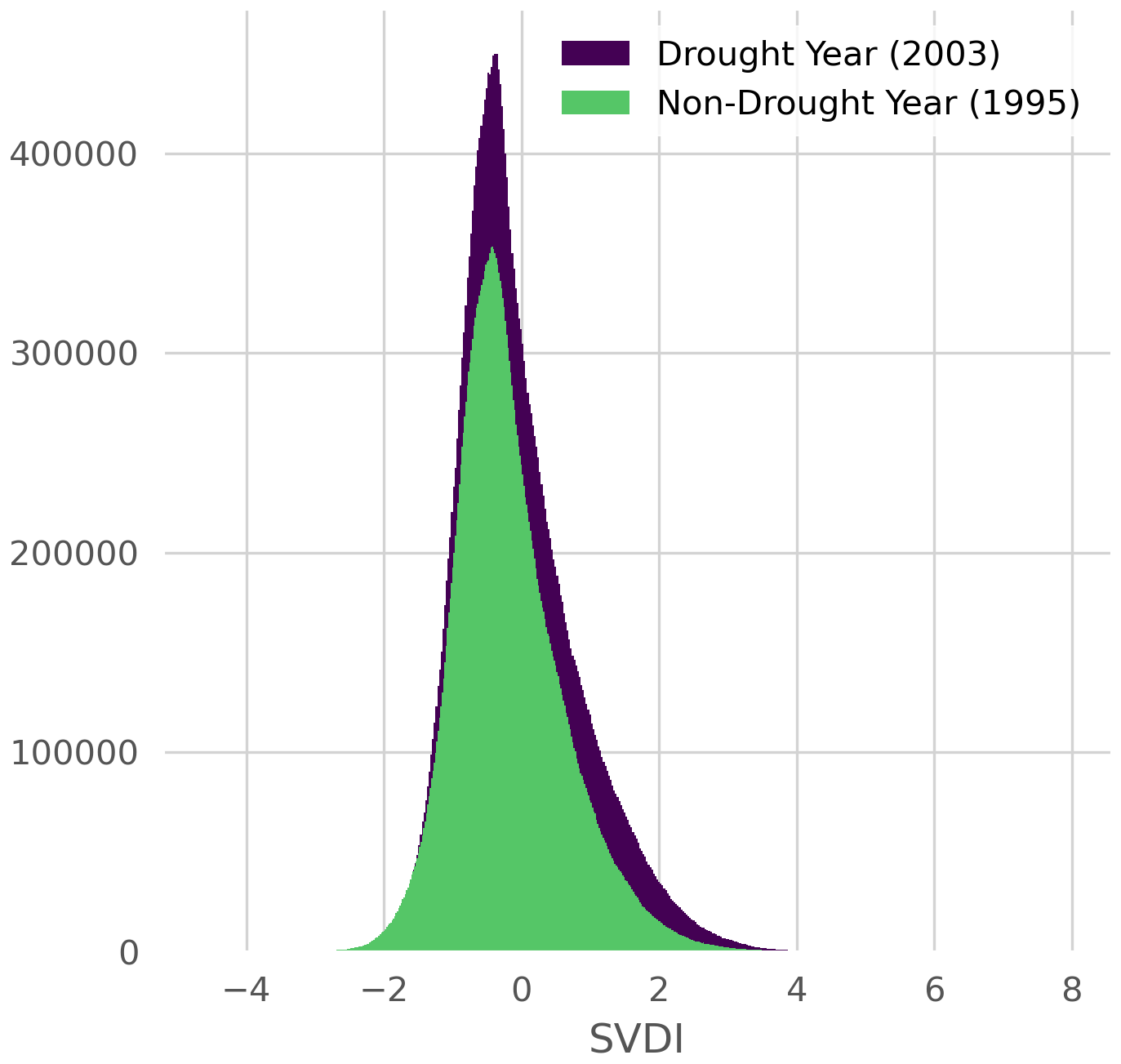
Figure 1 Histogram (counts) of SVDI for the year 2003 in which a major drought event occurred compared with the year 1993 without a major drought event.

2.2 Level 1: Space-time k-means for Intensity Clustering

2.2.1 Standard k-means

The standard workhorse for clustering is the k-means algorithm discussed in MacQueen (1967) and is formally described as follows. Consider a matrix $\mathbf{X}\in {\mathbb{R}}^{d\times n}$ that describes the dataset $\mathit{\{}{\mathit{x}}_i{\mathit{\}}}_{i=\mathrm{1}}^n$ with n instances of d-dimensional datapoints. The aim is to assign each datapoint to one of the k clusters whose centroids $\mathit{\{}{\mathit{c}}_j{\mathit{\}}}_{j=\mathrm{1}}^k$ are described as the matrix $\mathbf{C}\in {\mathbb{R}}^{d\times k}$. This assignment is described by the matrix $\mathbf{W}\in {\mathbb{R}}^{n\times k}$ where each element $w_{ij}\in \mathit{\{}\mathrm{0},\mathrm{1}\mathit{\}}$ and $\forall i,{\sum }_{j=\mathrm{1}}^k{w}_{i,j}=\mathrm{1}$. The k-means optimization problem that solves for both cluster assignment and cluster centroids consists of the following minimization:

$$\begin{array}{}\text{(1)}& {\mathrm{argmin}}_{W,C}\sum _{j=\mathrm{1}}^k\sum _{i=\mathrm{1}}^n{w}_{ij}d({\mathit{x}}_i,{\mathit{c}}_j),\end{array}$$

where d is a distance metric of choice. This standard k-means applied to SVDI values indexed in space and time, results in space-time agnostic clustering solely based on SVDI intensity. Standard k-means creates clusters that are stratified along SVDI intensities as shown on the right plot of panel (a) in Fig. 3. Due to the temporal dynamics of SVDI, the corresponding cluster assignment (with thresholding effect) results in a location rapidly transitions between clusters over time, as seen in the bottom plot of panel (b) in Fig. 2. These rapid time shifts are nonphysical. Hence, we propose to incorporate space-time information into the standard k-means as described in the following section.

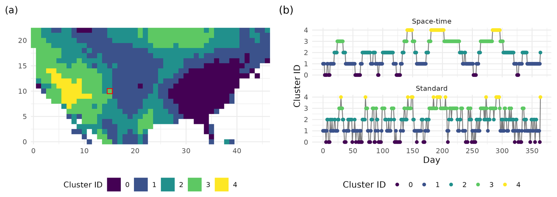
Figure 2 (a) Spatial extents of the five extracted clusters from the newly introduced space-time minibatch k-means on 2 June 2003. (b) Time series of cluster assignments showing drought regimes and their transitions for 2003 for space-time k-means (top), and standard minibatch k-means (bottom), of the region highlighted in red in (a).

2.2.2 Proposed Space-time k-means

In the following, the distance in Eq. (1) d(x,c) is based on a spatiotemporal neighborhood of x in order to account for spatiotemporal information in the cluster assignment and description. Note that d can be any chosen distance, here we base it on the Euclidean distance and modify Eq. (1) as follows:

$$\begin{array}{}\text{(2)}& {\mathrm{argmin}}_{\mathbf{W},\mathbf{C}}\sum _{j=\mathrm{1}}^k\sum _{i=\mathrm{1}}^n{w}_{ij}{\displaystyle \frac{\mathrm{1}}{\left|N\right({\mathit{x}}_i\left)\right|}}\sum _{{\stackrel{\mathrm{̃}}{\mathit{x}}}_i\in N\left({\mathit{x}}_i\right)}d({\stackrel{\mathrm{̃}}{\mathit{x}}}_i,{\mathit{c}}_j)\end{array}$$

where N(x_i) is a spatiotemporal neighborhood of the space-time datapoint x_i and $\left|N\right({\mathit{x}}_i\left)\right|$ is the cardinality of the neighborhood N(x_i). In this work, due to the spatiotemporal nature of the data, the neighborhoods constitute of adjacent spatiotemporal datapoints. The neighborhood size is determined by the correlation strength of these adjacent spatiotemporal datapoints, see implementation details in Sect. 3.1.2. One can envision general neighborhoods defined according to different criteria in the context of dependent data and not restricted to spatiotemporal data, as for instance in multivariate contexts. However, this exploration is left for future work. Finally, this heuristic equalizes all points' contributions in the neighborhood of x_i, each neighborhood point could be weighted according to its proximity to x_i. This was explored in the early stages and not pursued due to low improvements compared to the increased number of tunable parameters.

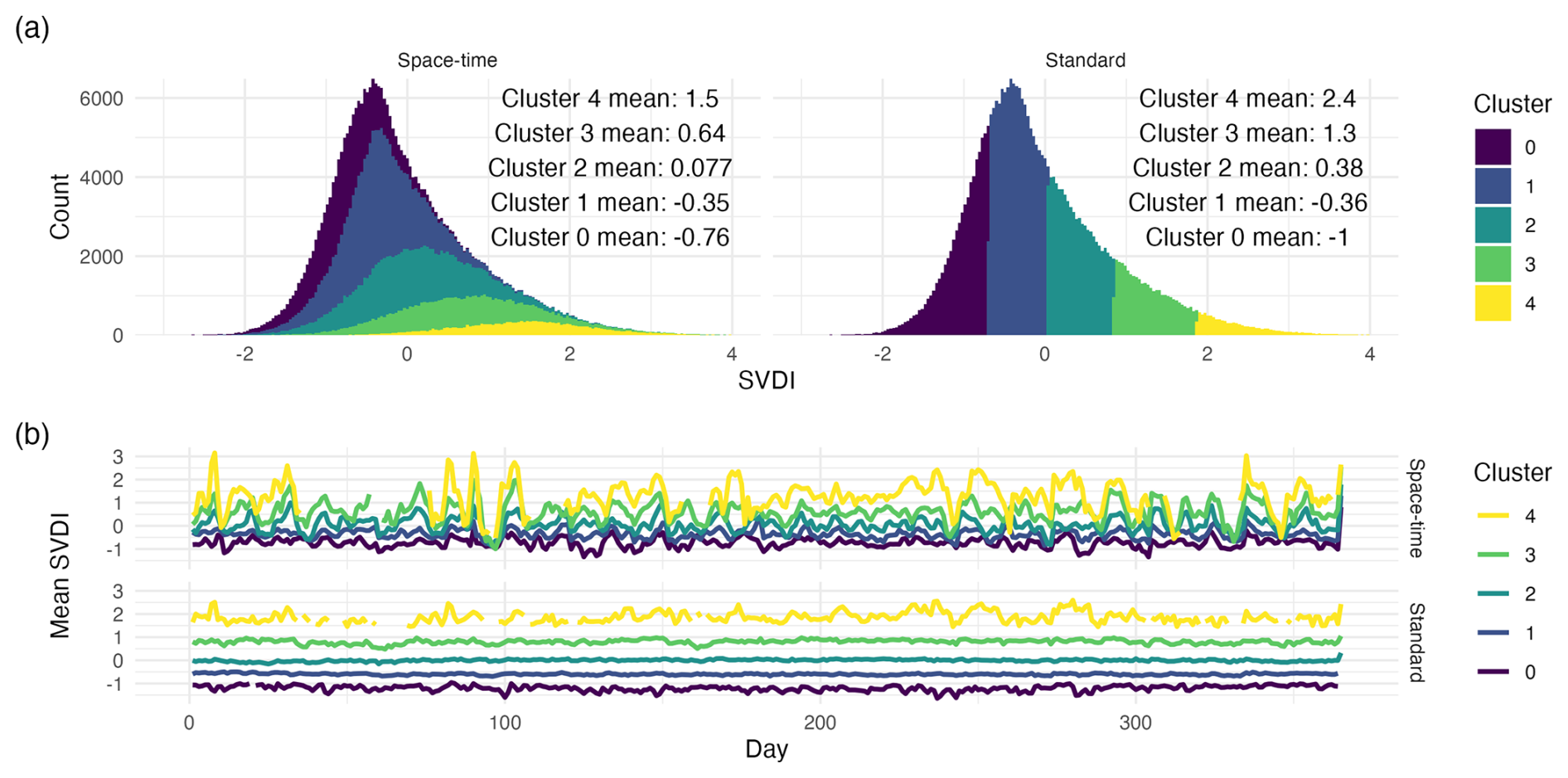
Figure 3 Panel (a) shows histograms between the new modified space-time k-means (left) and standard k-means (right). Panel (b) shows daily centroid means for the corresponding clusters found using the proposed space-time minibatched k-means (top), and standard minibatched k-means (bottom).

The top plot in panel (b) of Fig. 2 illustrates the benefit of using a space-time neighborhood, where now temporally consistent regimes are formed with realistic regime durations and transitions between drought regimes. With traditional k-means, the within-cluster variance is minimized regardless of space-time information, leading to clustering based on non-temporal mean and variance intensities, which creates rapid transitions between drought regimes due to the nature of the data. With the addition of the spatiotemporal k-means assignment, temporal durations and transitions better reflect physical drought evolution with more persistent regimes. This persistence is realistic when drought behaviors are considered as locations do not transition between drought states instantly. This new spatiotemporal assignment removes the stratification in the clusters distributions seen in the top right panel of Fig. 3, and blends out the boundaries between clusters by enabling cluster centroids and cluster assignment to depend on spatiotemporal information (top left panel of Fig. 3). In bottom panel (b) of Fig. 3, time series of k-means centroids exhibit different behaviors from the standard to space-time k-means. Each cluster centroid created using the standard k-means has stratified means with no overlap between clusters and small ranges of values. Moreover, these standard k-means centroids exhibit few changes in their temporal dynamics. With the proposed space-time k-means, cluster centroids can vary significantly in their range of values but also in their temporal dynamics. This behavior reflects a more flexible clustering algorithm to capture a variety of behaviors.

2.2.3 Minibatched k-means

For high-dimensional data (i.e., for large n) where X do not fit in memory, the minimization will take an unreasonable time to converge. To circumvent this, the minibatched k-mean iteratively performs the optimization of the k-means cost function (Eq. 1) over random batches of the data, making it greedy but also faster to converge (Sculley, 2010). In the following, all k-means procedures are performed by minibatching to tackle the large amount of data.

2.2.4 Expert-based Step: Drought Severity Assignment

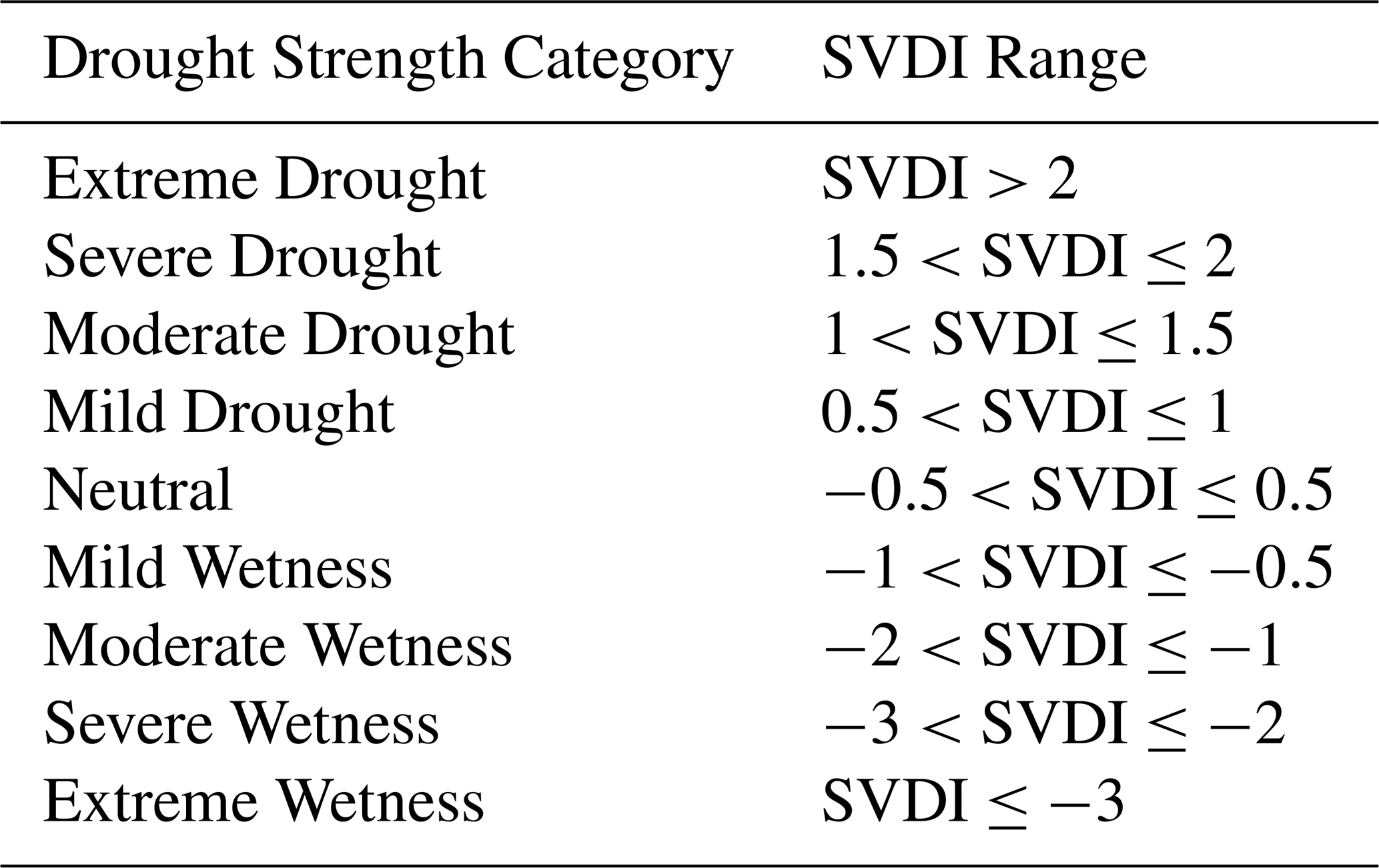
This step is specific to the studied application and can be omitted depending on the application. However, it enables to select a reduced number of clusters to be processed by DBSCAN and potentially creates regions with lesser datapoint density, hence enabling more potent DBSCAN step. After the space-time k-means step, cluster means are computed to determine drought severity. We perform a finer classification based on cluster-mean intensity following Table 1, similar to the dry and wet categories employed by the standardized precipitation evapotranspiration index (SPEI) (Vicente-Serrano et al., 2010). We select clusters identified by the space-time k-means whose cluster's mean is greater than 0.5, corresponding to mild, moderate, severe and extreme droughts. These selected clusters are passed to the next step to separate individual events. Clusters with means belonging to the same drought category were collapsed into a larger single cluster.

Table 1 Drought severity categories based on ranges of SVDI.

2.3 Level 2: Event-level Clustering

As a final step, we choose the density-based spatial clustering of applications with noise (DBSCAN) algorithm (Ester et al., 1996) to separate individual events from the previously extracted space-time k-means clusters. Indeed, Fig. 7 shows drought intensity clustering in a spatiotemporal consistent way; however, space-time points with similar statistical properties belong to the same cluster although they are spatially far apart and most likely pertain to different drought events. DBSCAN is a density-based algorithm that clusters points based on high- and low-density regions, hence accounting for their closeness to other high-density regions in the data domain. DBSCAN requires a distance function for which we used a normalized Euclidean distance, but any distance can be chosen. The modifiable parameters in DBSCAN are ϵ and n_min, where ϵ determines the minimum distance between neighbors, and n_min determines the minimum number of points required to form a dense region and start a cluster. Ultimately, DBSCAN finds the fewest number of clusters while requiring every pair of points in each cluster to be reachable within radius ϵ. A description of the algorithm is as follows.

• 1.

  Start with an unvisited point, mark it as visited, and find all its neighbors within a radius of ϵ:

  • –

    If more than the minimum number of neighbors (n_min) within the radius ϵ are found, the visited point is assigned as a core point,

  • –

    If not, then the point is considered as non-core. It is assigned to a cluster if there is one within radius ϵ, otherwise it is temporarily classified as a noise point,

• 2.

  If a core point is found in the previous step, a new cluster is started with this core point and all its density-reachable points (neighbors) are added to this cluster. Density-reachable points are points that can be reached via any sequence of intermediate neighbors within a distance ϵ (also called path of connected core points),

• 3.

  Repeat until all points are visited.

DBSCAN was chosen for this step as it does not require an a-priori number of clusters and creates clusters of arbitrary shapes based of datapoint local densities, hence enabling to identify individual drought events. Specifically, it creates separate clusters that have similar statistical properties (for instance drought-like) but spatially separated. DBSCAN is applied to each cluster extracted from Level 1 to obtain individual spatiotemporal individual drought events. While n_min was left fixed, ϵ was tuned in a similar fashion to k to create distinct and well-separated drought clusters that reflect known historical drought conditions. Before further analysis of these drought clusters, we trim the drought events of negligible size (i.e, having volume below the value of the parameter trim_volume). Note that ST-DBSCAN could have been used in this step; however, we found that the standard DBSCAN provided expected results, most likely because space-time structures are handled during the first space-time k-means step. Moreover, ST-DBSCAN requires tuning four parameters, reducing the control and interpretability of the algorithm.

3 Results and Discussion

In the following, we exemplify the algorithm parameter tuning on the historical drought of 2003, then we analyze the clustering performance of a known drought in 2000. Finally, we analyze statistics and long-term trends of the extracted space-time drought clusters.

3.1 Parameter Tuning for Clustering of Historical Drought of 2003

3.1.1 Historical Drought of 2003

We choose the summer 2003 droughts in the United States as our comparison criteria for parameter tuning. In 2003, there were two identified drought events. One drought was located in the central United States and the other in the Southwest. We focus on the evolution of the 2003 drought in the central United States (https://www.ncei.noaa.gov/access/monitoring/monthly-report/drought/200313, last access: January 2025), see Fig. 4a, because this region has been prone to extreme flash drought events over the last 40 years (Christian et al., 2019; Edris et al., 2023). In their review, (Lisonbee et al., 2021) highlighted two known constants in identifying a flash drought: rapid intensification and short duration. Thus, the 2003 drought event has been classified as a flash drought due to its rapid intensification (Otkin et al., 2018; Liu et al., 2020; Lisonbee et al., 2021; Edris et al., 2023) beginning in late June, and short duration, with a rapid demise and ending before September (Chen et al., 2019; Christian et al., 2019; Gamelin et al., 2022). The proposed algorithm has a total of six tunable parameters. We discuss the role each plays in the algorithm and their tuning on these historical data.

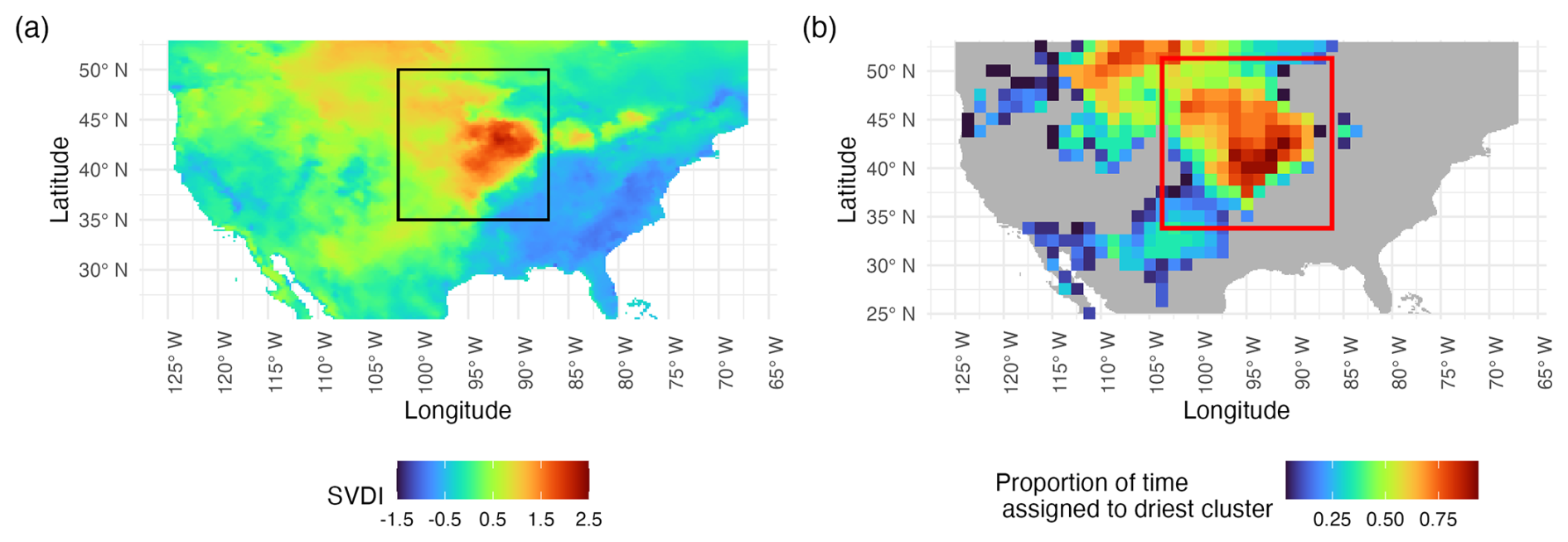
Figure 4 Panel (a), which is a recreation of Fig. 1 from Gamelin et al. (2022), shows the average SVDI for the month of August 2003. The spatial extent of the 2003 summer flash drought is given by the black bounding box. The region between latitudes 95 and 87° W of and longitudes 37.5 and 45° N within the bounding box shows the area of peak intensity of the 2003 central US Drought. Panel (b) shows the results of the proposed space-time clustering. The color is the proportion of days assigned to the driest space-time k-means cluster during August 2003. The red bounding box marks the approximate area of the 2003 summer flash drought over the period 1 July to 3 September 2003. Note that the resolution is different from one panel to another as (a) shows SVDI in its original spatial resolution and (b) shows results of the proposed k-means performed on downsampled data as described in this section. The same color palette as in Gamelin et al. (2022) is used.

3.1.2 Spatiotemporal Neighborhood

First, as the spatial region is large and covered at fine resolution, we downsample the grid by retaining every 10 grid-points to reduce the overall number of points while still remaining true to the spatial structure present in the full dataset.

Next, we define space-time neighborhoods for the proposed modified space-time k-means. We base space-time neighborhoods on the spatiotemporal correlation of SVDI. Spatiotemporal neighborhoods are centered around each datapoint and consist of points having non-zero space-time correlation with the neighborhood center point. Temporal autocorrelations decreased quickly within a week's lag time, as shown in Fig. 5. Thus, we choose a temporal neighborhood of 14 d (day) window around each datapoint (i.e., 7 d before and 7 d after the datapoint). On average, SVDI spatial correlations become negligible after around 127 km (kilometers) (not shown here), thus we choose circular spatial neighborhood of that radius.

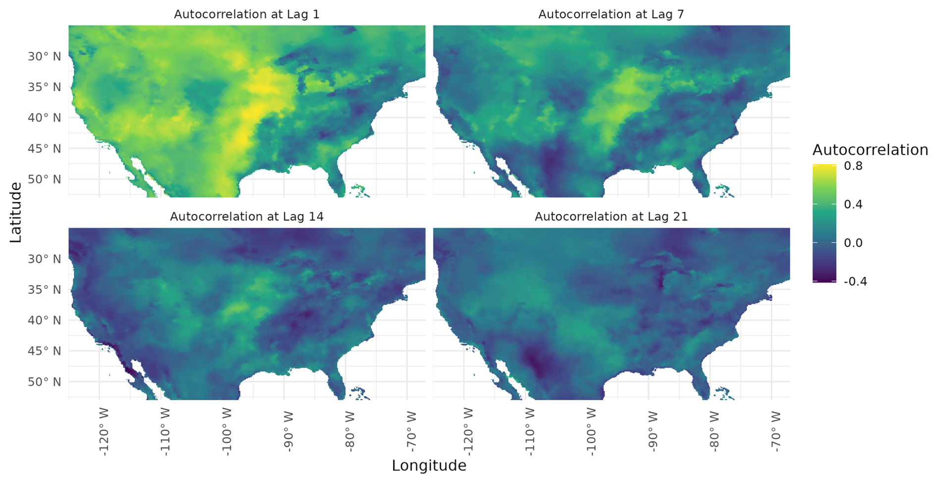
Figure 5 Point-wise SVDI temporal autocorrelation values at lag times of 1, 7, 14, and 21 d (clockwise starting at the top-left corner) during the summer.

Finally, we explore the joint effect of the spatiotemporal neighborhood's size on the accuracy of the associated clustering. Specifically, we evaluated how well different sizes of spatiotemporal neighborhoods created clusters that aligned with the historical drought of 2003, as shown in Fig. 6. The bounding box represents the observed extent of the 2003 flash drought. The latitudes extend from 35 to 50.5° N and the longitudes from −100.5 to −85.5 °W. Increasing the temporal window in the spatiotemporal neighborhood increases the number of points assigned to the driest cluster, while increasing the spatial neighborhoods spatially smooths the cluster assignments. The spatial neighborhood of 0.02 radians (around 120 km) and temporal neighborhood of 7 d aligned with similar patterns to the ones as seen in Fig. 4.

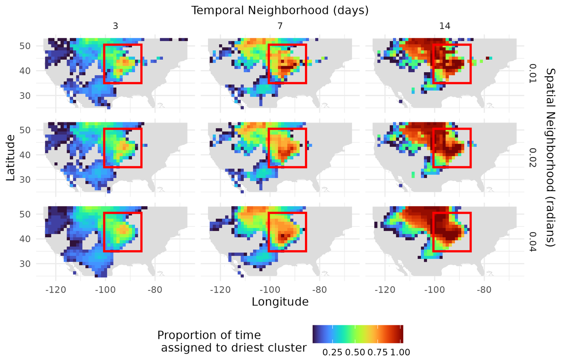
Figure 6 Proportion of points assigned to the driest cluster during the 2003 drought with spatial windows 0.01, 0.02, 0.04 radians (60, 120, and 240 km) (rows) and temporal windows of 3, 7, 14 d (columns). The bounding box correspond to the approximate area of the known drought, with latitudes from 35 to 50.5° N and longitudes from −100.5 to −85.5 °W.

3.1.3 Number of k-means Clusters

After choosing spatiotemporal neighborhoods, the number k of clusters in the proposed space-time k-means has to be selected. The value of k is related to the spanned range of intensity of drought and how well the clusters correspond to known drought events. In situations without ground truth, scores such as silhouette, presented in Rousseeuw (1987), Davies-Bouldin index, presented in Davies and Bouldin (1979), and Calinski-Harabasz index, presented in Calinski and Harabasz (1974), are used to assess clustering quality for a range of values of k, typically trading off inter- and intra-cluster properties. In practice, these scores are combined with domain knowledge to select a suitable value of k. In our case, domain knowledge alone was sufficient to find k that created clusters that aligned with the known drought. We inspected several values of k to see how well they spatially corresponded to the areas of known drought in the central United States during the 2003 drought. Following this, it was empirically chosen to work with k=5 clusters for this dataset. Figure 7 illustrates several time snapshots of the algorithm using five spatiotemporal clusters and the spatiotemporal neighborhood defined above. The newly proposed spatiotemporal k-means mirrored the development of the 2003 central US drought event, which is partially shown in panel (a) of Fig. 4. The region is absent of drought-identified clusters beginning in September as reported in literature (Gamelin et al., 2022). Additionally, in panel (b) of Fig. 4, which shows the results of the space-time k-means clustering, the red bounding box represents the known drought area from 1 July to 2 September 2003. Within this bounding box, the area assigned to the driest cluster during the month of August corresponds to the location of peak intensity identified in Fig. 1 of Gamelin et al. (2022) recreated in panel (a). From the five space-time k-means clusters, we assign these into four distinct drought clusters each corresponding to a single drought severity category (mild, moderate, severe and extreme) from Table 1. For 2003, only two of five SVDI cluster means were identified as drought and moved to DBSCAN. Cluster 4 with a mean of 1.44 and Cluster 3 with a mean of 0.644 were considered moderate and mild drought, respectively. Within these two drought categories, we prioritized tuning DBSCAN parameters to the cluster corresponding to moderate drought. While it may seem redundant to start with 5 spatiotemporal k-means clusters to condense down to 4 drought severity categories, the number of k-means clusters actually creates more resolution in identifying drought spatiotemporal events from the data and associated observed severity. Specifically, running the initial k-means with fewer clusters leads to larger clusters mismatching with known distinct spatiotemporal events of different severity.

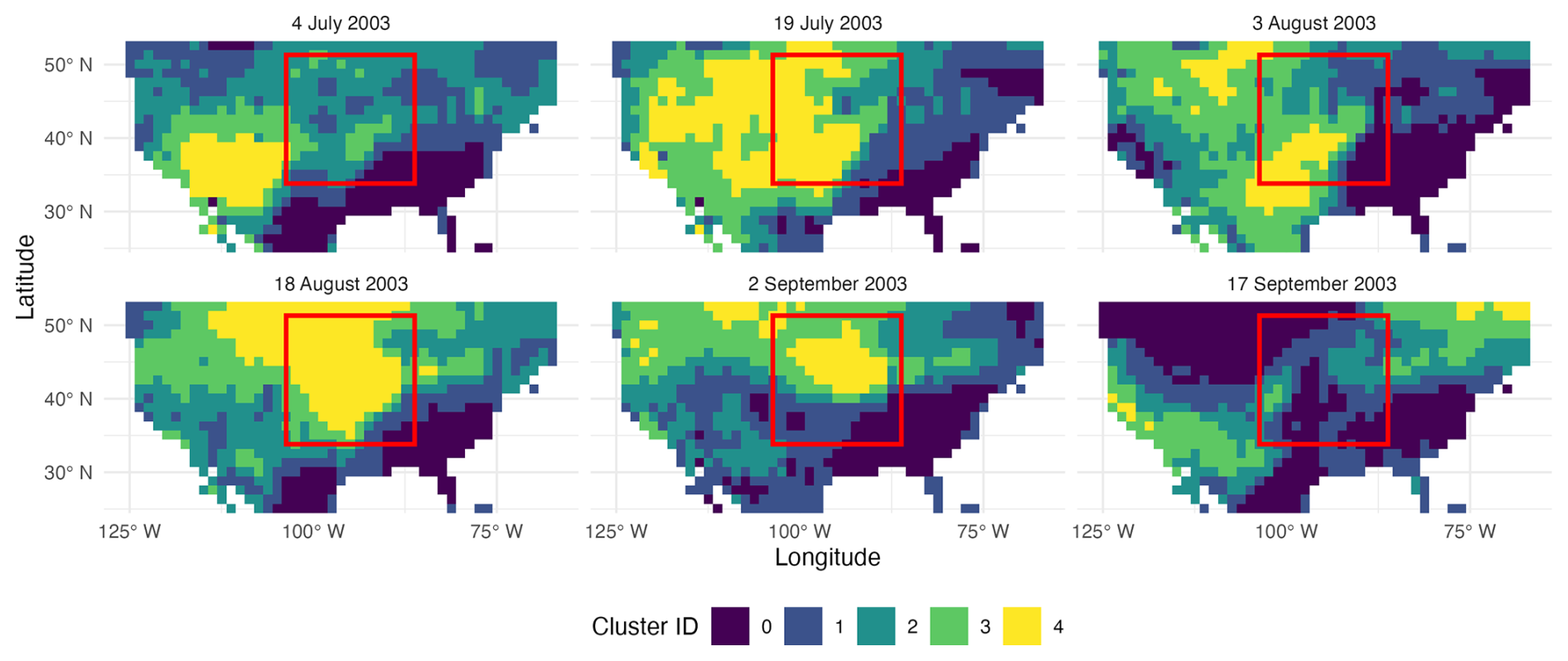
Figure 7 Maps of the spatial extent of the five space-time k-means extracted clusters in two-week intervals between July and September 2003. The red bounding box indicates the approximate known area of the 2003 central US flash drought over the period 1 July to 3 September 2003.

3.1.4 DBSCAN Tuning

Once the value of k is selected, the next parameters to tune are ϵ related to the distance between clusters and n_min (minimum cluster size) in DBSCAN, and trim_volume (minimum volume of space-time clusters).

We select ϵ by inspecting the space-time clusters along a range of values. Once these space-time clusters are found, we compare drought centroid evolutions for sufficient spatial and temporal overlap for each cluster to determine whether they should be consolidated into the same drought event. n_min, which controls the minimum cluster size around core points during cluster creation, was fixed at a value of 5.

Finally, trim_volume is the final tuning step for DBSCAN; it controls the minimum volume (500) of any space-time clusters. This parameter is related to ϵ; depending on ϵ small drought clusters may be classified as part of a larger cluster, remaining in the final space-time cluster since they surpass the minimal allowable volume indicated by trim_volume parameter.

Figure 8 shows the effects on cluster shapes of a range of ϵ values. Low values of ϵ result in space-time clusters that are stratified regardless of their spatiotemporal structures. As we increase the value of ϵ, we notice that three distinct space-time clusters emerge: one early in the year in the Southwest, a second one in the middle of the year also in the Southwest, and a large drought in the southwestern and central US spanning the remainder of the year. A small window of ϵ results in three distinct clusters. Once that threshold is passed, the smaller southwestern cluster is subsumed into the larger cluster. Finally, too high values of ϵ result in a single cluster. Overall, the effect of ϵ also shows the robustness of the space-time clusters – aside from the unrealistic clusters seen for low values of epsilon – the general structure of the space-time clusters remains consistent across a given range of ϵ. Ultimately, we choose ϵ=0.25 as it best represents the general trends in the known droughts of 2003. Figure 9 illustrates the individual events identified with these parameters for the moderate and mild categories. We note that the mild drought has a larger spatiotemporal extent than the moderate one corresponding to physical expectations.

Figure 8 Effect of different values of ϵ on DBSCAN clusters in 2003.

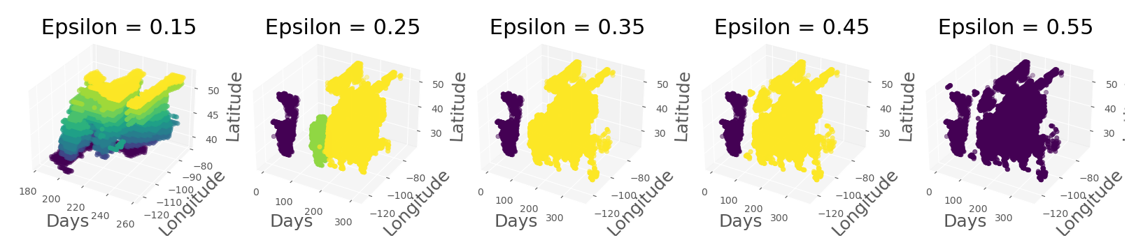
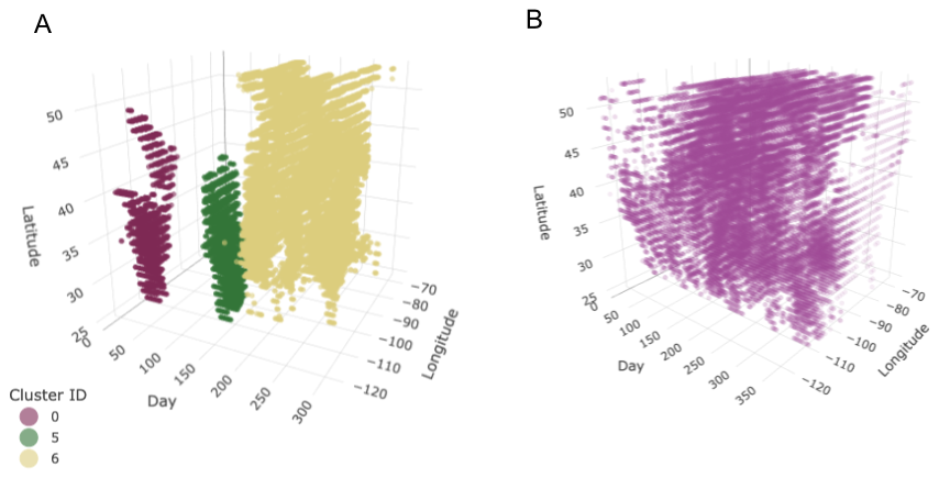
Figure 9 Distinct drought clusters found for the year 2003 for and moderate (a) and mild (b) drought severity categories.

Figure 10 shows the spatial centroids of the 2003 clusters, labeled by their pentad (5 d interval) number and linked with directional arrows to indicate their space-time propagation. With ϵ=0.25, moderate-drought Cluster 5 (purple) is contemporaneous to the larger drought cluster, moderate-drought Cluster 6 (yellow), but is considerably spatially separated and properly assigned to a different clustering according to historical records. In this case, the decision to consider moderate-drought Cluster 5 as distinct, rather than include it alongside the larger drought moderate-drought cluster, informed our selection of ϵ, but highlight the ability of the method to separate clusters of the same severity into different events as needed.

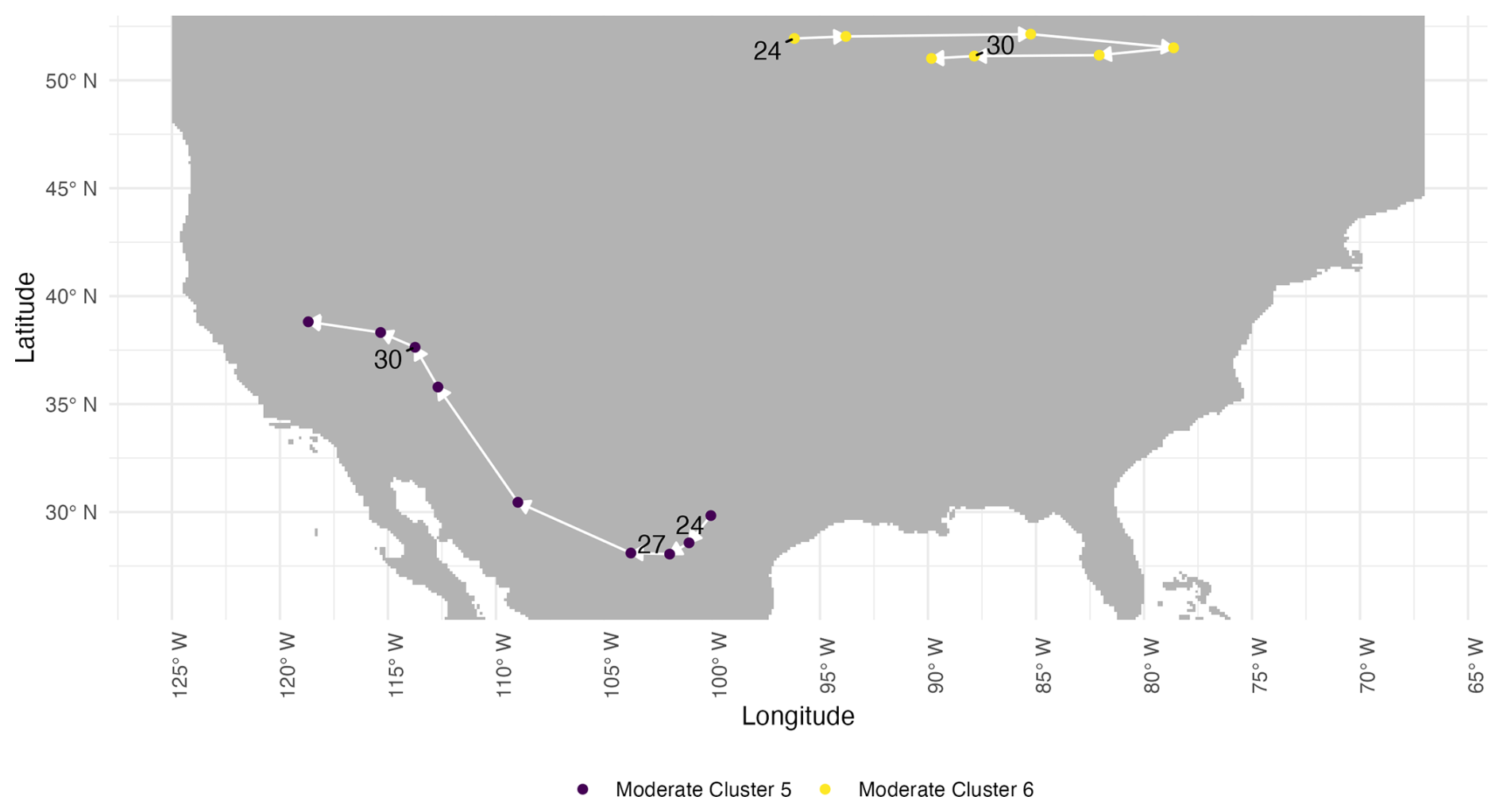
Figure 10 Spatial trajectories of centroids for Clusters 5 (purple) and 6 (yellow) representing individual moderate drought events shown in Fig. 9 over pentads 24 to 32 in 2003.

Finally, to explore within cluster dynamics, we assign to each grid point a drought severity based on the value of SVDI from Table 1. This refined partition allows us to investigate developing drought within each drought category. In Fig. 11, the histogram displays aspects of the development of the 3 moderate drought clusters in 2003 (between dashed black lines). The height of the bar provides an idea of the spatial extent of the drought, with taller bars indicating more spatial points involved in the drought. The color fill of the bars indicates the drought severity. The color of the frame (black, green and yellow) of each bar indicates cluster assignment, hence different drought events.

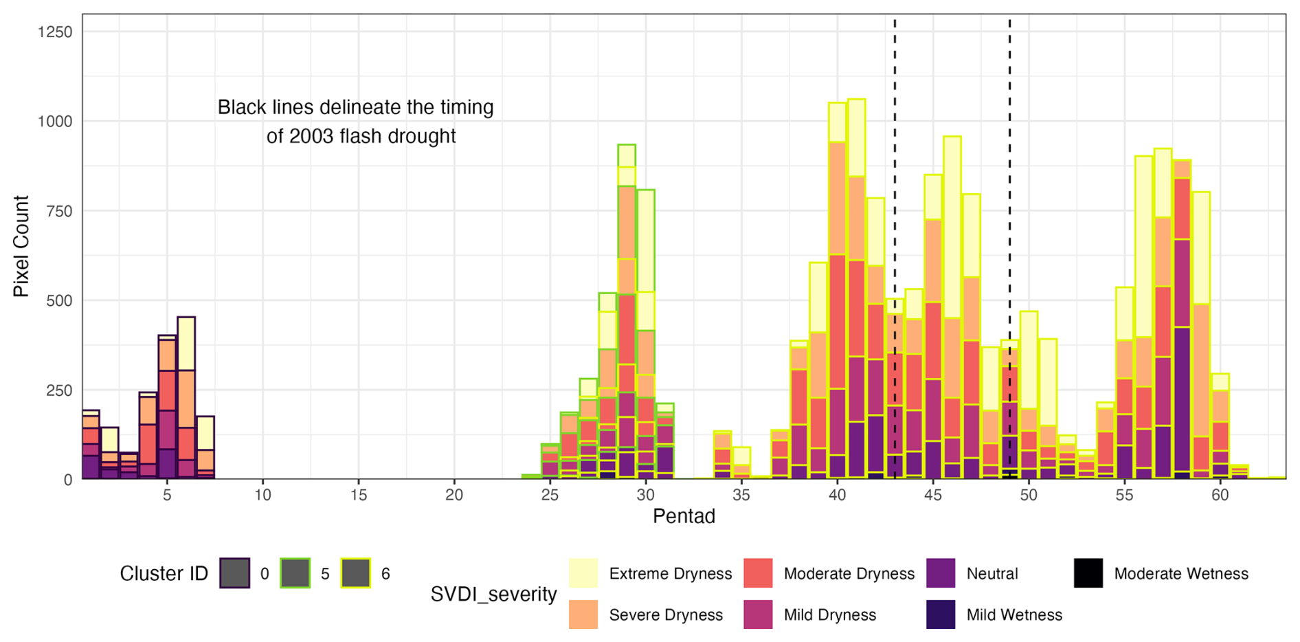
Figure 11 Stacked histogram showing the number of grid points experiencing different severity of droughts and their temporal development for the 3 spatiotemporal drought clusters for 2003 (between dashed black lines). The color of the outline (black, green and yellow) of each bar indicates cluster assignment.

In the drought progression snapshots shown in Fig. 12, the 2003 summer drought is captured by Cluster 6 of moderate drought (yellow). Moderate-drought Cluster 6 also contains components of a flash drought that occurred in the American Southwest prior to the summer 2003 central US flash drought, which can be observed in the peak in the histogram around pentad 45 of Fig. 11. In both the drought progression spatial snapshots in Fig. 12 and the drought progression histogram in Fig. 11, the 2003 flash drought event is associated within a larger drought event and does not stand out in Cluster 6, highlighting the potential difficulty in capturing spatiotemporally smaller drought events, like flash droughts, occurring within a larger-scale drought.

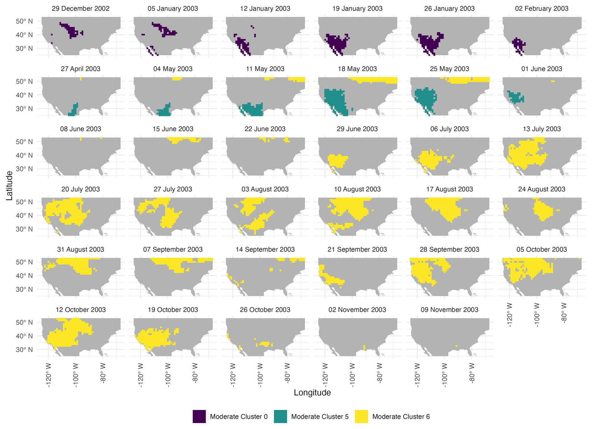
Figure 12 Weekly evolution of the three individual moderate drought events with different colors across the year 2003. Weeks are labeled by the starting date of that week.

3.2 Analysis of Clustered Droughts in 2000

To further demonstrate the performance of the clustering algorithm, we apply the proposed bi-level clustering approach to identify drought events in 2000 with SVDI. In the following, we investigate two settings of the clustering: (1) we tune the clustering algorithm to the year 2000 data and (2) we keep the parameters tuned to 2003, and apply the corresponding clustering procedure to the unseen year 2000 that also contained a historical drought. This second step enables to test the applicability of the tuned method to unseen data. The year 2000 has a well-documented summer flash drought that originated in Florida, Mississippi and Georgia in the southeastern United States. Simultaneously, there was a longer-term drought occurring in Texas, the Plains and Southwest that increased in intensity and spatial area from July through October. The historical development of the southeastern flash drought is shown in the supplemental figures of Gamelin et al. (2022), republished in Fig. 13.

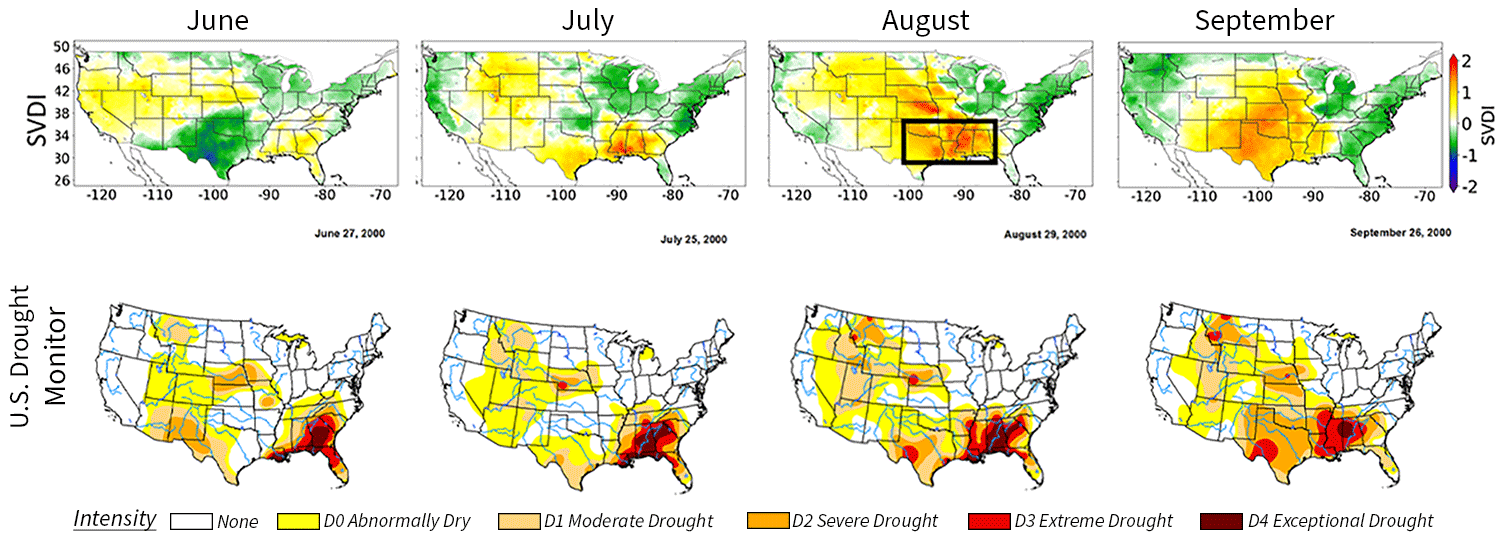
Figure 13 Reprinted from Gamelin et al. (2022, supplementary Fig. S1). SVDI monthly averages (bottom) for June, July, August, and September in 2000 alongside corresponding monthly United States Drought Monitor snapshots (top). The black bounding box encloses the area of the 2000 flash drought.

When the algorithm's parameters are tuned to the year 2000, the associated space-time clustering correctly captures the timing and spatial location of the historical 2000 drought, see Fig. 14 (top panels in yellow) compared to Fig. 13. With these parameters, the extracted drought is classified as extreme. This figure shows the weekly location of the extracted drought cluster during the summer of 2000, starting from July and ending in October. For this tuning case, the same space-time neighborhood and number of clusters in the k-means steps was kept the same and only the ϵ was tuned in the DBSCAN step.

In comparison, with 2003-tuned parameters, the 2000 drought is classified as severe (less severe than extreme) and was captured in one of the severe drought space-time clusters, as seen in Fig. 14 (bottom panels in purple). The spatiotemporal cluster correctly places the area of drought in the southeast in early July. However, the cluster misidentified the drought in late July and early August, conflating the drought with a contemporaneous drought in Texas and across the Plains. This misidentifying only lasted for around 2 weeks before shifting back to approximately the right location in the week of August 8th onwards, mirroring the historical flash drought once more. The issues with the misidentification of the flash drought were completely rectified above by tuning the DBSCAN parameters to the year 2000 specifically (top panels in yellow) as observed above. Additionally, it is worthwhile to mention that the misidentification issues that arose from applying 2003-tuned parameters to 2000 could be due to the smoothness of SVDI. Sometimes, a lack of spatial separation in SVDI values is observed, as in Fig. 13, linking areas experiencing different drought events. In this figure, although the area in the flash drought is highlighted, a large portion of the West is spatially linked through a high SVDI with the area of flash drought. Overall, although the parameters were tuned for a completely different year, the resulting space-time clustering provided a fairly accurate representation of the flash drought in 2000, highlighting the robustness of the proposed clustering method. However, as observed here, drought severity classification may be under- or over-estimated when spatiotemporal clusters differ from one method to the other.

Figure 14 Weekly evolution of extracted historical drought cluster from the proposed method corresponding to 2000 summer flash drought. Top: Clusters resulted from tuning method to 2000 specifically, classified as extreme. Bottom: Clusters found using algorithm parameters tuned to 2003 and classified as severe. Colored areas show the extracted droughts.

3.3 Long-term Drought Statistics

We investigate trends in long-term drought patterns based on the clusters extracted by the proposed algorithm over the 42-year time period. The algorithm is applied to each year separately with the 2003-tuned parameters. Figure 15 displays the evolution across the 42-year time period of the annual mean SVDI in all space-time drought clusters categorized by their severity. To further compare the drought characteristics of the extracted clusters, several descriptive statistics are calculated at the cluster and annual levels. The calculated statistics are based on drought intensity, duration, and timing. The intensity is calculated as the average SVDI in each cluster. Duration and timing are based on the number of days classified as drought. For all annual statistics, each statistic is first calculated for each identified drought cluster, and then averaged across clusters. Mild and moderate droughts dominate in the first half of the time frame, whereas during the latter half severe and mild droughts predominate, as observed in Fig. 15. Additionally, the frequency of mild droughts has increased over time. While there are years with no mild drought between 1981 and 2000, there has been a mild drought almost every year between 2000 and 2021. Figure 16 shows the annual average duration of space-time droughts for each severity category. Average drought duration demonstrates trends: after 2000, mild droughts are more likely to last the entire year, while also becoming more frequent. Severe droughts are lasting longer, while occurring more frequently than moderate drought. Finally, the longest extreme drought from this dataset occurred during 2011.

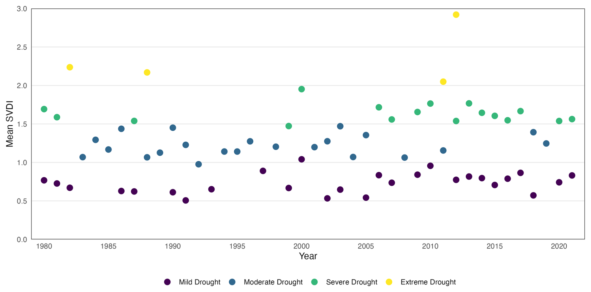
Figure 15 Annual mean SVDI across extracted space-time drought clusters over all 42 years for each drought severity category.

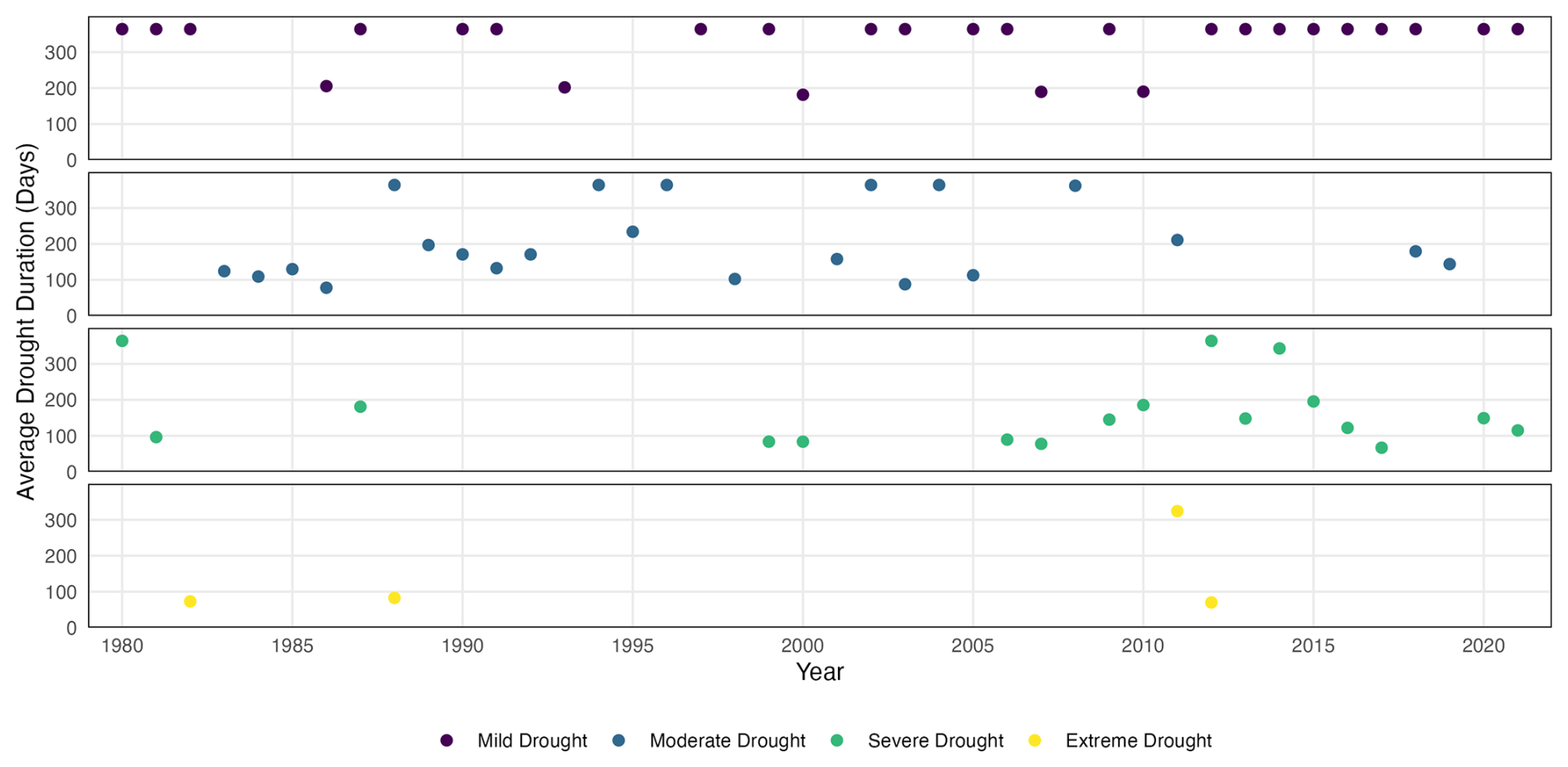
Figure 16 Annual average drought duration across extracted space-time drought clusters over all 42 years for each drought severity category.

4 Conclusions

Our proposed space-time extension of k-means allows for efficient and flexible clustering while incorporating space-time information. Generally, the proposed algorithm can separate a dataset into different intensity categories based on their value and spatiotemporal structures, an ability that standard k-means lacks. When applied to the SVDI drought index, our algorithm improves on standard k-means by (1) creating temporally persistent drought regimes with realistic transitions, (2) creates spatiotemporally consistent drought events, (3) ability to capture historically accurate clusters that capture known drought events. Additionally, the proposed clustering method was tested on unseen data (year 2000) that are not used during the tuning phase (year 2003) and was able to identify droughts in an unrelated year with reasonable accuracy. This indicates the robustness of the proposed method across different data. Finally, the drought trends identified through applying our space-time algorithm to the 42-year time period reveal shifts in drought across the United States. These shifts correspond to known trends in droughts (Leeper et al., 2022; Strzepek et al., 2010).

Part of the method's flexibility centers around the parameters that can be tuned for different research aims. For example, time scales for the temporal neighborhood can be adjusted to detect short- or long-term events, and the size of the spatial neighborhoods could detect large- or small-scale events. Due to this flexibility, the proposed space-time clustering can be used to assess numbers of spatiotemporal continuous phenomena besides droughts. Moreover, the proposed bi-level procedure enhances the spatiotemporal interpretability over existing spatiotemporal clustering and reduces the computational burden compared to relying on a single clustering method. Since the proposed method relies on two clustering techniques, future research directions could incorporate other methods in place of either k-means or DBSCAN, including Hierarchical Density-Based Spatial Clustering of Applications with Noise (HDBSCAN) (Campello et al., 2013), Balanced Iterative Reducing and Clustering using Hierarchies (BIRCH) (Zhang et al., 1996), or Voronoi Clustering (VoroClust) (Winovich et al.(in revisions, 2024). All of these methods are unsupervised clustering methods that have additional capabilities compared to DBSCAN. HDBSCAN allows for clusters of differing densities by performing a DBSCAN algorithm with several values of ϵ. BIRCH locally clusters over subsets of the data, providing faster clustering speeds than DBSCAN. VoroClust uses Voronoi tessellation to quickly capture complex clustering patterns on large multidimensional datasets with computational times faster than DBSCAN, HDBSCAN, and BIRCH. These methods work well with high-dimensional data, potentially extending the spatiotemporal clustering ability into higher dimensions.

Finally, the procedure highlights the challenges of working in an unsupervised environment where interpretable steps and domain experts are required. Developing ways to automate the algorithm tuning towards specific environmental phenomenon is a worthwhile future goal.