Simulation of extreme functionals in meteoceanic data: application to surge evolution over tidal cycles

We investigate the influence of time-varying meteoceanic conditions on coastal flooding under the prism of rare events. Focusing on conditions observed over half tidal cycles, we observe that such data fall within the framework of functional extreme value theory, but violate standard assumptions due to temporal dependence and short-tailed behavior. To address this, we propose a two-stage methodology. First, we introduce an autoregressive model to reduce temporal dependence between cycles. Second, considering the model residuals, we adapt existing techniques based on Pareto processes. This allows us to build a simulator of extreme scenarios, by applying inverse transformations. These simulations depend on an initial time series, which can be randomly selected to tune the desired level of extremes. We validate the simulator performance by comparing simulated time series with observations, through several criteria, based on principal component analysis, extreme value analysis, and classification algorithms. The approach is applied to the surge data, on the Gâvres site, located in southern Brittany, France.

1 Introduction

Events like Johanna and Xynthia, which led to flooding on the Atlantic coast of France in 2008 (Le Roy et al., 2015) and 2010 (Bertin et al., 2014), respectively, illustrate the potentially devastating effect that storms can have on the coasts by generating significant surges and waves, in combination with high tides. Coastal flooding is particularly concerning because coastal zones are densely populated and host high-value activities (Dawson et al., 2009). This concern is expected to grow in the coming decades, as projections estimate that between 2.1 and 2.9 billion people will live in near-coastal areas by 2100 (Reimann et al., 2023). Consequently, improving the forecasting of such events has become a critical objective for public authorities (Toimil et al., 2017).

Numerical hydrodynamic simulators provide essential insights into the complex relationship between coastal flooding and extreme meteoceanic conditions. In this study, we focus on extreme surge-induced flooding (Chaumillon et al., 2017) but with the added complexity that the governing conditions are time-varying and evolve over tidal cycles (3 h around the tidal peak). In our context, the challenge lies in the fact that the inputs to the numerical models are time-dependent functions, i.e., functional inputs, and our goal is to generate extreme time series. When the inputs are functional, extreme value analysis is usually applied to a set of scalar variables that summarise the extreme aspect of the whole series. Then, in order to obtain an entire extreme time series, simulations of these scalar values are combined with either a schematic pattern (Nicolae Lerma et al., 2018) or a normalized storm time series. Yet, the approach is highly sensitive to the chosen pattern (Rohmer et al., 2018). To overcome this issue, we adopt a functional extreme value analysis framework which has been applied in particular to extreme windstorms, heavy spatial rainfall and temperature (de Fondeville and Davison, 2022; Ferreira and de Haan, 2014; Chailan et al., 2014).

To simulate extreme data, we aim to construct a probabilistic model for these time series. However, applying the theory of functional extremes typically requires two main assumptions:

1. The time series must be independent and identically distributed (i.i.d.).

2. The time series should exhibit regular variation in the sense of Clémençon et al. (2024), which implies heavy-tailed marginals.

Unfortunately, these assumptions are hardly met in many situations of interest for coastal and ocean engineering; see for instance the study by Mackay et al. (2021) for the problem of dependence, and see that of Sando et al. (2024) for an example where the extreme distributions of waves do not exhibit regular variation. This is also the case for the surge time series analysed in our case in France (full details are provided below in Sect. 2), which motivated this study. The temporal dependence is usually treated by applying an extremal declustering (Ferro and Segers et al., 2003), which means that exceedances are grouped into clusters and only the maximum from each cluster is retained. Since observations separated in time by more than τ are assumed independent, this procedure returns a sequence of independent maxima. Yet, we choose not to adopt this approach as, first, it depends on the choice of the parameter τ and, second, we aim at providing a widely applicable method. To overcome these limitations, we propose to proceed in two steps:

1. Temporal dependence is addressed using an autoregressive model, which captures inter-cycle dependence while preserving intra-cycle structure.

2. To recover heavy-tailed marginals, we apply the approach of Opitz et al. (2021), combining a semi-parametric model of the empirical distribution with a Fréchet marginal transformation.

Following this preprocessing stage, and under an additional joint tail condition detailed in Sect. 2.2.2, the transformed time series satisfy the requirements for functional extreme modeling. We then build a probabilistic model following the framework in Dombry and Ribatet (2015), which relies on a polar coordinate representation (Kokoszka et al., 2019) whose components asymptotically follow a Pareto process.

This probabilistic model allows us to simulate extreme time series by first sampling from that Pareto process, then applying inverse transformations to recover time series in the original space. This is made possible thanks to the independence between the tidal cycles obtained from the autoregressive process. In this context, our method offers two notable advantages. First, by accounting for the temporal dependence between observations, it provides a generator of independent extreme residuals. Second, since these simulations depend on an initial time series used to invert the autoregressive model, the level of extremeness can be tuned through the choice of the reference series. This flexibility enables a range of applications – from data-like simulations, that follow the same law as extreme observations, to sequences of consecutive extreme events. A special care is paid to assess the quality of our simulated extremes by proposing a series of tools including Principal Component Analysis (PCA), extreme value analysis and two-sample classification tests (Lopez-Paz and Oquab, 2016). The overall performance of the method is evaluated using the storm surge case study.

This article is organized as follows. In Sect. 2, we describe the context of our case study and analyze the characteristics of the observations. Section 3 details the two-stage methodology leading to the probabilistic model on functional data. Section 4 explains how this model is employed to simulate extreme data. Section 5 applies the full framework to the storm surge case study and evaluates the simulation results.

Implementation

The method is coded in R (R Core Team, 2023a) and relies on several packages. We first use the arima function from the R package (R Core Team, 2023b) to estimate the parameters of the autoregressive models. The POT (Ribatet and Dutang, 2022) and extRemes (Gilleland and Katz, 2016) packages are then used to analyze exceedances at each time step. The code for the marginal transformations is based on Opitz et al. (2021). Besides, we use the FactoMineR package (Lê et al., 2008) for PCA, VineCopula package (Nagler et al., 2023) to model the law of copulas and the mvtnorm package (Genz and Bretz, 2009) for iso-density curves. Finally, we use the e1071 (Meyer et al., 2023) and randomForest (Liaw and Wiener, 2002) packages to construct support-vector machines and random forest classifiers.

2 A motivating case study

2.1 Data description

From a physical point of view (Fig. 1), the coastal floods result from the combined effect of: mean sea level, tide (T), atmospheric storm surge (S, generated by the atmospheric pressure and wind) and waves (that generate an additional component of water level at the coast, called wave set-up, induced by wave breaking processes). Flood can result either from overflow (i.e. when the coastal water level at the coast, also called storm tide, exceeds the crest level of the coastal defenses) or overtopping (i.e. when storm tide level is lower than the crest level, but conditions are such that individual waves can overtop the coastal defenses). To simulate these processes, the most common approach is to use numerical hydrodynamic models that are forced, on their offshore boundaries by event-scale time series of: (1) water level resulting from the combination of mean sea level, tide and atmospheric storm surge, (2) wave conditions (height, period, direction, or the full wave spectrum). Within these forcing components, the mean sea level can be assumed constant at the storm event scale, the tide results from gravitational forces such that it is a predictable variable (see e.g. Pugh, 1987), while atmospheric storm surges and waves are more aleatoric, resulting from atmospheric conditions. Thus, efforts on generating extreme time series of forcing conditions should mainly focus on these two last components. In the present paper, as a first step toward this overall challenge, we focus on the univariate component, i.e. the atmospheric storm surge, rather than the wave components that are at least trivariate (height, period, direction). In addition, it should be noted that in many coastal environments the atmospheric surge has a larger contribution to the storm tide than the wave set-up (Idier et al., 2019).

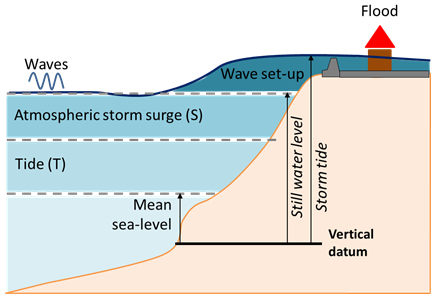
Figure 1 Water level components and forcing conditions of coastal hydrodynamic models. Adapted from Idier et al. (2019).

As a study case, we focus on Gâvres, located on the French Atlantic coast, which is particularly sensitive to coastal flooding. The town has been impacted several times in its history like in 1904 or in 1924 (Idier et al., 2020). Despite the evolution of its coastal defenses, about 120 houses were flooded during storm Johanna (8-10 March 2008) (Idier et al., 2020). We selected this case because: (1) hydrodynamic models are in place and validated, (2) a dataset of continuous offshore meteoceanic conditions (used as forcing conditions for the hydrodynamic models) has been built, covering the 1900 to 2016 period (see Idier et al., 2020). This dataset includes time series of: mean sea-level, tide, atmospheric surge, wave (height, period, direction) and local wind, with a 10 min temporal resolution. Focusing on atmospheric storm surge, it has been built by combining results from simulations done using a depth-averaged hydrodynamic model over the 2008–2016 period (called MARC) with lower quality estimations of atmospheric storm surge on periods before 2008. As the location of the offshore boundary of the Gâvres hydrodynamic modelling chain is in water depth of about 50 m, the atmospheric storm surge can be estimated using the inverse barometer formula, which consists of a rise of the local water level in the presence of local low air pressure or vice versa (for more details, see e.g. Pugh, 1987). Thus, to cover the period before 2008, meteorological hindcasts as 20CR (Compo et al., 2015) and CFSR (Dee et al., 2014) were used and improved through a quantile-quantile (QQ) correction, using the MARC dataset as the reference. As the 20CR hindcast has a lower quality than CFSR hindcast, in the present paper, we focus on the 1979–2016 period (rather than considering the entire dataset from 1900 to 2016). In addition, it is important to account for the phasing with tide since the latter significantly controls the flood in most of macrotidal areas (as Gâvres). In this context, flood may occur when high tide levels are combined with large storm surges. Thus, in the present development, we will also consider tide information. In the dataset, the tide time series has been built based on the tidal components database FES2014 (Lyard et al., 2021), with an extraction point at less than 1 km away from Gâvres site. We thus concentrate in the following on atmospheric storm surges conditions over half tidal cycles, occurring within ±3 h around high tide, such that, for each tidal cycle, focusing on the ±3 h time window around the high tide, we have time series of length 37. Over the 1979–2016 period, this corresponds to 26 652 time series, each representing a tidal cycle, that will be what we call “observation” in what follows.

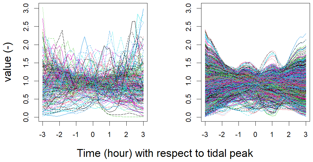
Traditionally, analyses focus on time series that follow a consistent pattern. For instance, in Tendijck et al. (2024), all the time series considered are centered around a peak of significant wave height. On the contrary, the time series in our dataset do not exhibit a specific shape (Fig. 2). We will use the notation $X_M^t$ to describe the value obtained at time t for the Mth tidal cycle. Thus, $X_M^{\mathrm{1}},\mathrm{\dots },X_M^{\mathrm{37}}$ represents the time series associated with the Mth tidal cycle.

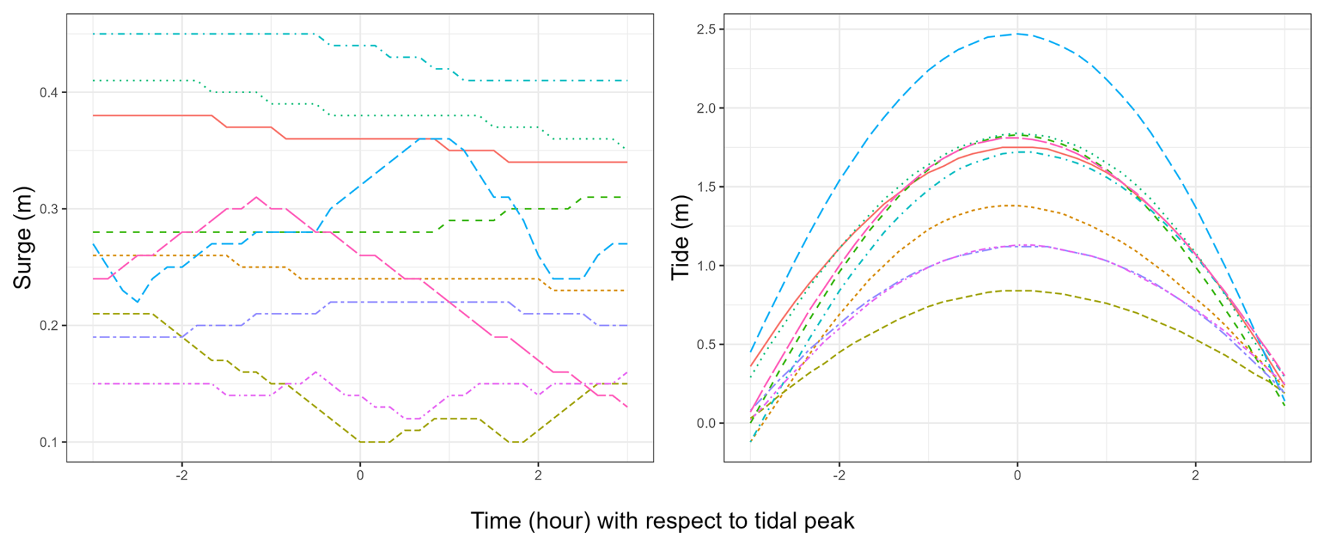
Figure 2 Sampling of 10 observations from 1979 to 2016 for surge S (left) and for tide (right).

We study the time series that distinguish themselves by an extreme behavior. This trait refers to the framework of extreme functionals, which is based on some assumptions discussed in the next section.

2.2 Two issues with the standard assumptions

2.2.1 Correlated observations

We generally assume that the observations (here time series of length 37) are i.i.d (Dombry and Ribatet, 2015), which implies that, for all $t=\mathrm{1},\mathrm{\dots },\mathrm{37}$, the series ($X_{\mathrm{1}}^t,\mathrm{\dots },X_N^t$) with N the number of observations should constitute an i.i.d sample. However, as illustrated by the autocorrelogram ACF and the partial autocorrelogram PACF at time t=1 (Fig. 3), we observe that the time series are correlated for each value of t. The correlation level is around 0.10 when the lag in terms of tidal cycle index equals 50. Besides, we observe that the time series are cross-correlated as for instance $X_M^{\mathrm{1}}$ is correlated with $X_{M+h}^{\mathrm{2}}$ (see Appendix A1).

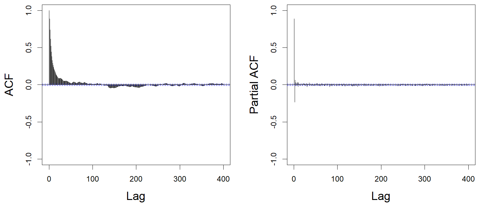
Figure 3 Time series analysis of the surge at the first time step of each event (t=1) with a lag in terms of tidal cycle index: ACF (left panel); PACF (right panel). The dotted blue lines correspond to the confidence interval in case of a Gaussian white noise.

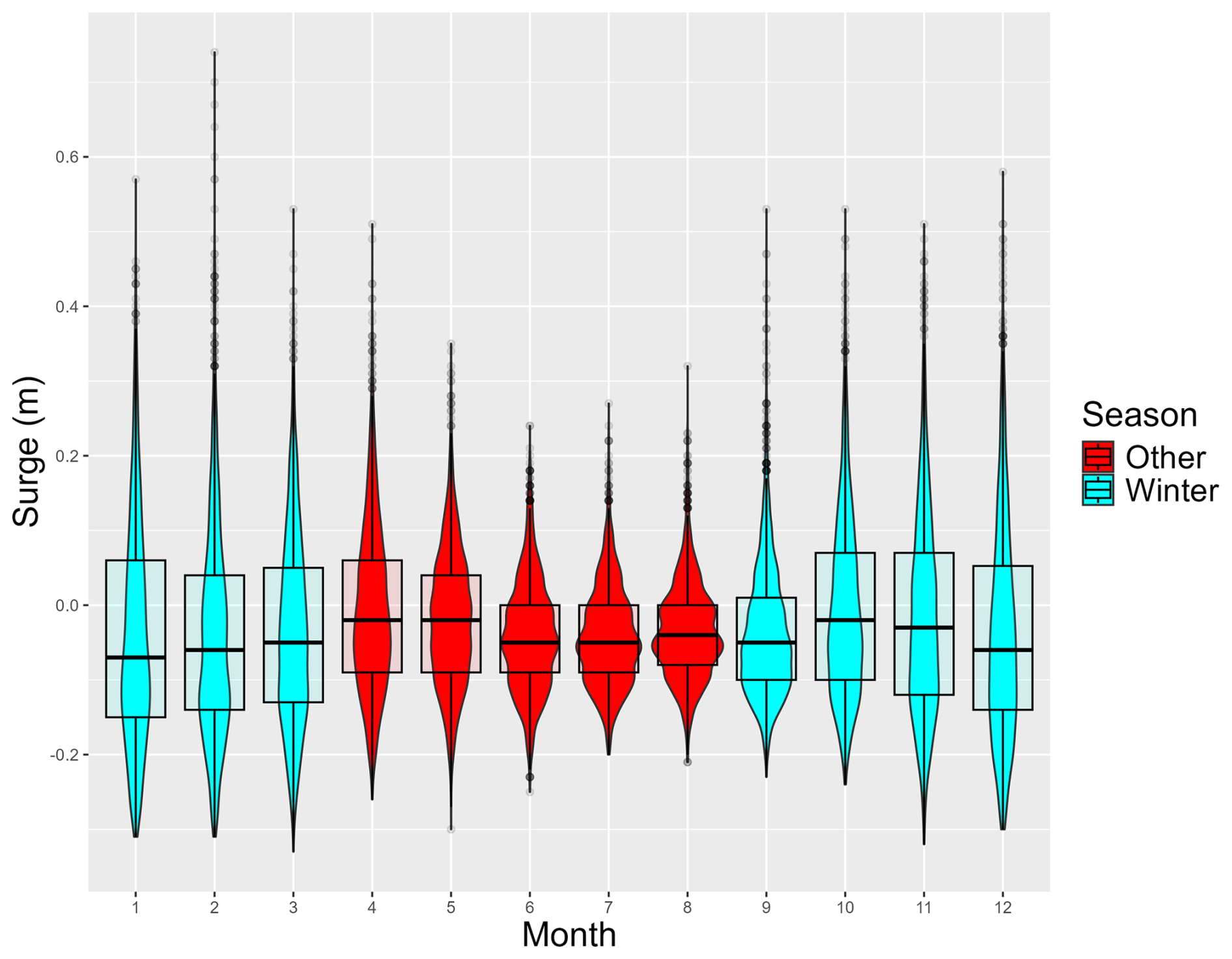
In addition to these strong correlations, we observe a seasonality of the variable with higher values observed during Winter months (September–March) (see Appendix A2). In conclusion, the independence assumption is rejected.

2.2.2 Departure from the regular variation hypothesis

In this paper, we consider that time series are realizations of a stochastic process X_M whose sample paths belong to some Hilbert space E (Clémençon et al., 2024). Using the notation $\stackrel{w}{⟶}$ for weak convergence of probability measures, we say that X_M is regularly varying with index α>0 if there exist normalizing constants a_n→∞ and some measure μ on E\{0} such that

$$n\mathbb{P}(a_n^{-\mathrm{1}}{\mathit{X}}_M\in .)\underset{n\to \mathrm{\infty }}{\stackrel{w}{⟶}}\mathit{\mu }(.),$$

and μ is homogeneous:

$$\mathit{\mu }\left(cA\right)=c^{\mathrm{-}\mathit{\alpha }}\mathit{\mu }\left(A\right),c>\mathrm{0}.$$

Note that this definition implies, by Proposition (3.1) of Clémençon et al. (2024), that for each t, the law of $X_M^t$ exhibits asymptotic Pareto-type decay with index α. To properly define this concept, we recall some prerequisites in extreme value theory. Let U be a univariate random variable and assume that U lies in the attraction domain of a so called Generalized Extreme Value (GEV) law (Balkema and De Haan, 1974; Ferreira and de Haan, 2014). This means that, for a n-sample $U_{\mathrm{1}},\mathrm{\dots },U_n$ following the law of U, there exists constants $a_n>\mathrm{0},b_n$ such that

$$M_n:=\underset{i\in \left[\right[\mathrm{1},n\left]\right]}{max}{\displaystyle \frac{U_i-b_n}{a_n}},$$

and M_n converges in distribution to a GEV law. Then, when we consider the exceedances of U over a high threshold u – the so-called Peak-Over-Threshold (POT) approach –, we obtain a Generalized Pareto distribution (GPD):

$$\begin{array}{}\text{(1)}& \mathbb{P}(U\le x\mid U>u)=\left\{\begin{array}{ll}\mathrm{1}-{\left(\mathrm{1}+\mathit{\gamma }\frac{x-u}{\mathit{\sigma }}\right)}^{-\frac{\mathrm{1}}{\mathit{\gamma }}}& \mathrm{if}\mathit{\gamma }\ne \mathrm{0}\\ \mathrm{1}-\exp (-\frac{x-u}{\mathit{\sigma }})& \mathrm{otherwise},\end{array}\right.\end{array}$$

where x>u verifies $\mathrm{1}+\mathit{\gamma }\frac{x-u}{\mathit{\sigma }}>\mathrm{0}$. We denote this law $\mathrm{GPD}(u,\mathit{\sigma },\mathit{\gamma })$ and F_GPD the corresponding cumulative distribution function (cdf), where γ,σ are respectively shape and scale parameters. Within the framework of regular variation, the law of $X_M^t$ exhibits Pareto-type decay for every value of t, corresponding to the case $u=\mathit{\sigma }/\mathit{\gamma }$, with $\mathit{\gamma }=\mathrm{1}/\mathit{\alpha }>\mathrm{0}$ in Eq. (1). Following the peak-over-threshold approach (Coles et al., 2001), the extremeness of a time series is quantified by a homogeneous functional ℓ, which maps the time series to a scalar value. This function is referred to as a cost functional (Dombry and Ribatet, 2015) or a risk functional (de Fondeville and Davison, 2022). A time series is classified as extreme if the corresponding value of ℓ exceeds a specified threshold. Defining the risk function as $\mathrm{\ell }\left(\mathit{f}\right)=\left|\right|\mathbb{I}(\mathit{f}>\mathrm{0})\mathit{f}|{|}_{L^{\mathrm{2}}}$, we analyze the extremes of ℓ(X_M). As we estimate the evolution of γ according to the number of exceedances, we analyze the sign of the shape parameter γ (Fig. 4). The Hill estimator explored in De Haan and Resnick (1998) (dotted line) is based on a property of extreme observations under heavy-tail hypothesis (γ>0). If the assumption holds, the estimator converges. Since the plot shows no stable region for the Hill estimator, we conclude that the condition γ>0 is not met, which is confirmed by the moments and MLE estimators (straight and dashed line) analysed in Haan and Ferreira (2006). Hence, the regular variations assumption is not satisfied.

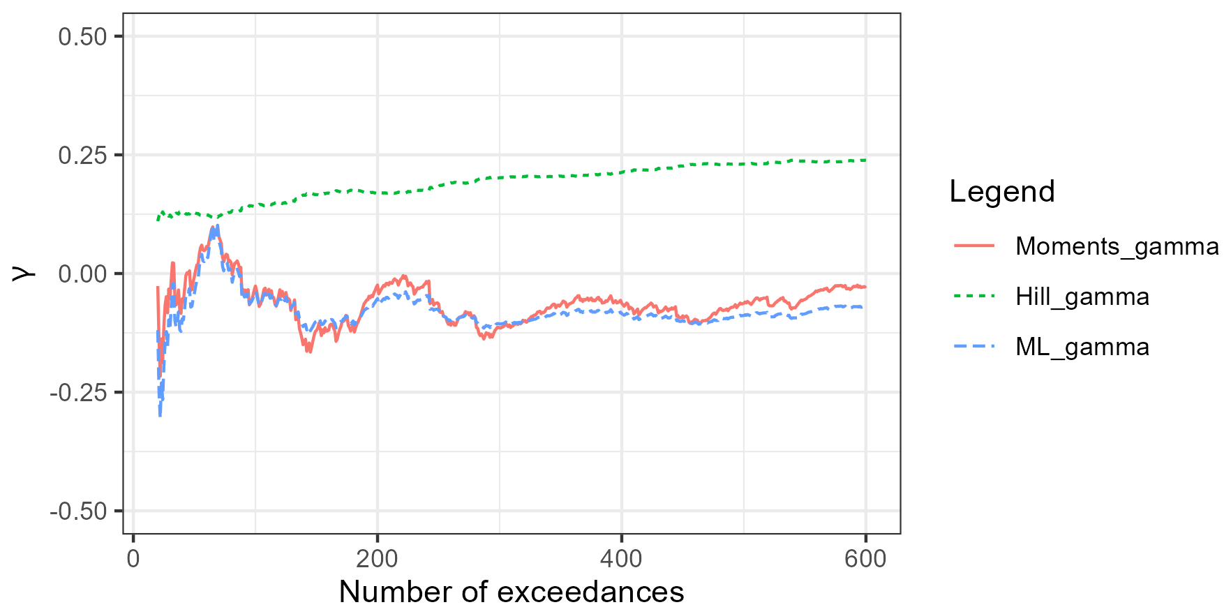
Figure 4 Estimated value of the GPD shape parameter γ with various methods (solid line: moments estimator, dotted line: Hill estimator, dashed line: MLE estimator).

3 Construction of a probabilistic model

As discussed in the introduction, we aim at building a simulator accounting for temporal dependence and short-tailed behaviour of the observations. Our methodology has two stages. The first stage is pre-processing and aims at solving the two issues raised in the previous section. It is divided in two steps. First, we obtain independent data by considering the residuals of an autoregressive model (“whitening” step). Second, starting from these residuals, we recover heavy-tail distributions by using marginal transformations. In a second stage, we construct a probabilistic model based on a polar coordinate representation. The flowchart of the whole methodology is summarized in Fig. 5. We further detail each step in the following.

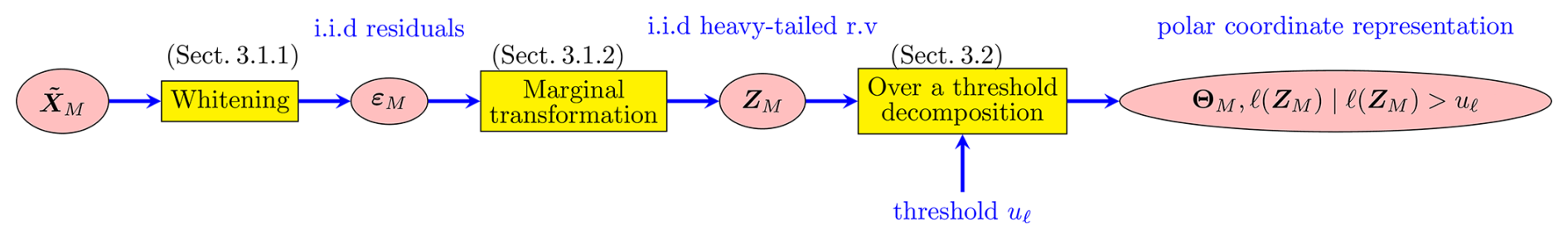
Figure 5 Construction of the polar coordinate representation from raw data (corresponding sections indicated near the boxes).

3.1 Preprocessing stage

3.1.1 Recovering the independence case: Whitening with an auto-regressive model

Starting from observed time series X_M, we aim at removing the temporal dependence between successive time series. We first detrend the data by simply writing

$$\begin{array}{}\text{(2)}& X_M^t={\mathit{\alpha }}_{t}M+c_t+{\mathit{\eta }}_M^t={\mathit{\alpha }}_{t}M+{\stackrel{\mathrm{̃}}{X}}_M^t,\end{array}$$

where α_t represents the slope, c_t is the intercept and ${\mathit{\eta }}_M^t$ is the residual term. The detrended time series is denoted by ${\stackrel{\mathrm{̃}}{X}}_M^t$. In practical applications, we need to subsample in the data by imposing a time step Δ between observations in order to reduce the temporal correlation, which is also known as declustering in the literature. Mathematically, we have $M=\mathrm{1}+\mathrm{\Delta }m$ with $m=\mathrm{1},\mathrm{2},\mathrm{\dots }$. Finally, for each value of t, we model the temporal dependence, with respect to M, by an autoregressive model, leading to

$$\begin{array}{}\text{(3)}& {\stackrel{\mathrm{̃}}{X}}_M^t={\mathit{\beta }}_{\mathrm{0}}^t+\sum _{i=\mathrm{1}}^p{\mathit{\beta }}_i^t{\stackrel{\mathrm{̃}}{X}}_{M-\mathrm{\Delta }i}^t+{\mathit{\epsilon }}_M^t,\end{array}$$

where ${\mathit{\beta }}_{\mathrm{0}}^t$ is a constant term, $({\mathit{\beta }}_i^t{)}_{i=\mathrm{1},\mathrm{\dots },p}$ are the model parameters and ${\mathit{\epsilon }}_{\mathrm{1}}^t,{\mathit{\epsilon }}_{\mathrm{1}+\mathrm{\Delta }}^t,\mathrm{\dots },{\mathit{\epsilon }}_N^t$ are the model residuals. These residuals form a white noise, i.e. are i.i.d. random variables, that we will now consider. The parameters are estimated by applying the least-squares on the residuals. This can be viewed as a conditional log-likelihood method under a Gaussian assumption. However, apart from this estimation stage, we do not impose a specific distribution for the residuals and more specifically, no assumptions about the tail of the distribution.

Remark

We propose here an approach based on autoregressive models that does not account for seasonality. This choice is justified in the present study, as the seasonal part of X_M can be easily removed by focusing on the Winter periods (see Sect. 5.1). Nevertheless, more sophisticated models incorporating seasonal components, such as SARIMA models (Dubey et al., 2021), could be considered. However, a limitation of these models is that they would require multiple initial time series to invert Eq. (3), which forms the basis of the generation method described in Sect. 4.2.2.

3.1.2 Recovering heavy-tailed distributions: Using a Fréchet marginal transformation

Starting from the residuals ${\mathit{\epsilon }}_M^t$ obtained in the previous step, we aim at obtaining a heavy-tailed distribution. A simple way to proceed is to use the transformation $\mathcal{T}:X\mapsto -\mathrm{1}/\log \left(F_X\right(X\left)\right)$ where X is a continuous random variable with cdf F_X. Indeed, 𝒯(X) follows a Fréchet distribution (which is heavy tailed). However, in our case, the cdf of ${\mathit{\epsilon }}_M^t$ must be estimated independently for each $t=\mathrm{1},\mathrm{\dots },\mathrm{37}$. Following Opitz et al. (2021), we approximate it by a mixture of the empirical cdf in the non-extreme part and a GPD distribution in the extreme region. Denoting F^emp the empirical cdf and F_GPD the distribution function of a GPD variable (Eq. 1), ${\widehat{F}}_{{\mathit{\epsilon }}^t}$ has the form

$$\begin{array}{}\text{(4)}& {\widehat{F}}_{{\mathit{\epsilon }}^t}\left(\mathit{\epsilon }\right)=\left\{\begin{array}{ll}{F}_t^{\mathrm{emp}}\left(\mathit{\epsilon }\right)& \mathrm{if}\mathit{\epsilon }<u^t\\ (\mathrm{1}-p_u)+p_u{F}_{\mathrm{GPD}(u^t,{\mathit{\sigma }}^t,{\mathit{\gamma }}^t)}\left(\mathit{\epsilon }\right)& \mathrm{otherwise},\end{array}\right.\end{array}$$

where p_u is a parameter and u^t verifies $p_u=\mathrm{1}-{\widehat{F}}_{{\mathit{\epsilon }}^t}\left(u^t\right)$. In the sequel, we will denote $Z_M^t=\mathcal{T}\left({\mathit{\epsilon }}_M^t\right)$.

3.2 Modeling stage based on a polar coordinate representation

We suppose that the model Eq. (3) enables to obtain independent joint vectors $\left(\right({\mathit{\epsilon }}_M^t{)}_{t=\mathrm{1},\mathrm{\dots },\mathrm{37}},\left({\mathit{\epsilon }}_{M+\mathrm{\Delta }h}^t{)}_{t=\mathrm{1},\mathrm{\dots },\mathrm{37}}\right)$. If it is not the case, we would need to apply a vector autoregressive model (VAR) (Juselius, 2006) on the vector $({\stackrel{\mathrm{̃}}{X}}_M^t{)}_{t=\mathrm{1},\mathrm{\dots },\mathrm{37}}$. Since the pre-processing stage produces a random process with heavy-tailed (Fréchet) marginals, it allows us to apply the framework introduced by Dombry and Ribatet (2015), which requires marginals with Pareto-type tails. In this setting, functional data are modeled using a polar decomposition of the form

$$\begin{array}{}\text{(5)}& \mathit{f}=\mathrm{\ell }\left(\mathit{f}\right)\times \mathit{A}\mathbf{\left(}\mathit{f}\mathbf{\right)},\end{array}$$

with f=Z_M in our case. The radius ℓ(f), chosen here as the L² norm of f, allows to define extremes of random elements in a Hilbert space E while A(f) represents the angular pattern of the function. Following Clémençon et al. (2024), let $E=L^{\mathrm{2}}\left(\right[\mathrm{0},\mathrm{1}\left]\right)$ denote the Hilbert space of square-integrable, real-valued functions. We assume that Z_M is a regularly varying random element of E with index α=1, in the sense of the definition provided in Sect. 2.2.2. Under this additional assumption, the components (ℓ(f),A(f)) become asymptotically independent, conditional on ℓ(f)>u_ℓ as u_ℓ→∞, and the conditional process $\mathit{f}/u_{\mathrm{\ell }}\mid \mathrm{\ell }\left(\mathit{f}\right)>u_{\mathrm{\ell }}$ converges in distribution. As a consequence, we have

$$\begin{array}{}\text{(6)}& \mathrm{\ell }\left(\mathit{f}\right)\textcolor{red}{}\mathit{A}\mathbf{\left(}\mathit{f}\mathbf{\right)}\left|\mathrm{\ell }\right(\mathit{f})>u_{\mathrm{\ell }},u_{\mathrm{\ell }}\to +\mathrm{\infty }.\end{array}$$

Thus, we must select a convenient threshold u_ℓ as defined in Eq. (6). Denoting ${\mathbf{\Theta }}_M={\mathit{Z}}_M/\mathrm{\ell }\left({\mathit{Z}}_M\right)$, one selection method is based on the convergence of the angular component ${\mathbf{\Omega }}_M=({\mathbf{\Theta }}_M\mid \mathrm{\ell }({\mathit{Z}}_M)>u_{\mathrm{\ell }})$ toward a spectral tail process (Segers et al., 2017). The main idea is to analyze the behavior of Ω_M as u_ℓ increases gradually (Clémençon et al., 2024). After choosing a sufficiently high threshold u_ℓ, we obtain the polar coordinate representation (${\mathbf{\Theta }}_M,\mathrm{\ell }\left({\mathit{Z}}_M\right)\mid \mathrm{\ell }\left({\mathit{Z}}_M\right)>u_{\mathrm{\ell }}$), which is used to simulate new extreme time series.

4 Simulation of extreme time series

We propose a two-step simulator of new extreme observations based on the probabilistic model. In the first step (Sect. 4.1), we model the law of the polar coordinates and use properties of Pareto processes to generate simulations of Z_M, denoted Z_sim. In the second step (Sect. 4.2), we apply reverse transformations to Z_sim to reconstruct time series of interest. We describe the complete method in Fig. 6, where the forward-pointing arrows represent the transformation step introduced in Sect. 3 whereas the backward-pointing arrows indicate the simulation phase. As previous sections describe the construction of the model, we now focus on the simulator derived from this representation.

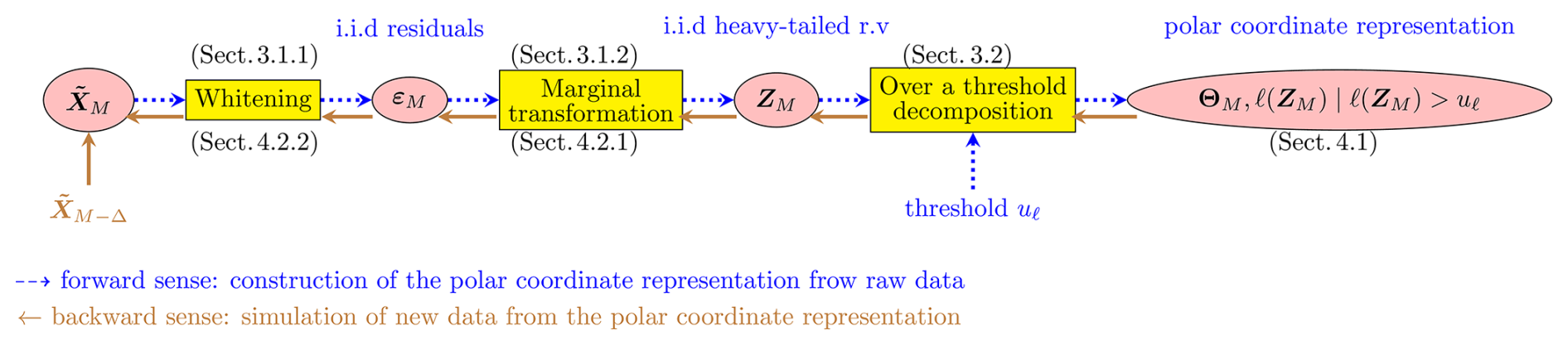
Figure 6 Two-stage methodology to simulate extreme time series (corresponding sections indicated near the boxes). The simulation starts from the left with the polar coordinate representation resulting from the forward sense (described in Sect. 3).

4.1 Modeling of polar coordinates

4.1.1 Functional analysis of the angular component

The simulation of extreme time series is based on the polar decomposition given in Eq. (5). Simulating the radial component ℓ(f) is straightforward as its asymptotic distribution is explicit (a Pareto distribution). In contrast, simulating the angular component A(f) is much more challenging. Several simulation methods have been proposed in the literature (de Fondeville and Davison, 2018), which rely on a spectral representation of the coordinate-wise maximum of $Z_M^t$ using Gaussian processes (Dombry and Ribatet, 2015). They all depend on the choice of a parametric model for the variogram. In contrast, we use a dimensionality reduction method, here PCA, before fitting parametric models. We follow Clémençon et al. (2024) by decomposing the standardized time series Ω_M in an orthonormal basis where (ν_j)_j≥1 are eigenvectors sorted by decreasing order of the eigenvalues (λ_j)_j≥1, (C_j)_j≥1 the PCA coordinates.

To reduce the dimensionality of the problem, we retain only the first J eigenvectors and denote by R_J the ratio of total inertia explained by the truncated basis. Applying the elbow rule (Perry et al., 2025), we truncate the PCA basis when adding another eigenvector does not significantly decrease (1−R_J). This dimensionality reduction step allows us to estimate only the joint distribution of the scores, enabling the simulation of new extreme observations.

4.1.2 Modeling the law of the angular component.

We account for the dependence between PCA coordinates by using the copula (Rüschendorf, 2009) C defined as

$$\begin{array}{}\text{(7)}& F(C_{\mathrm{1}},\mathrm{\dots },C_J)=\mathbf{C}\left(F_{\mathrm{1}}\right(C_{\mathrm{1}}),\mathrm{\dots },F_J(C_J\left)\right)=\mathbf{C}(v_{\mathrm{1}},\mathrm{\dots },v_J),\end{array}$$

where F is the joint distribution function of the vector $(C_{\mathrm{1}},\mathrm{\dots },C_J)$ and F_i is the distribution function of the ith marginal. We approach the joint law of $(v_{\mathrm{1}},\mathrm{\dots },v_J)$ by fitting a parametric copula model. Since many parametric copulas models are limited to the bivariate case, we use vine copulas (Czado and Nagler, 2022) when J>2, which use a tree representation of the dependence structure where each edge corresponds to a bivariate copula. Then, the law of the whole vector is modeled by combining the pairwise models in a hierarchical manner. Thus, this modeling approach captures multivariate distributions without requiring any assumption on the joint distribution of the entire vector $v_{\mathrm{1}},\mathrm{\dots },v_J$. To simulate new scores $C_{\mathrm{sim}}=(C_{\mathrm{sim},\mathrm{1}},\mathrm{\dots },C_{\mathrm{sim},J})$, we apply $F_i^{-\mathrm{1}}$ for $i=\mathrm{1},\mathrm{\dots },J$ to new values $({\stackrel{\mathrm{̃}}{v}}_{\mathrm{1}},\mathrm{\dots },{\stackrel{\mathrm{̃}}{v}}_J)$ sampled from the model. With this method, we generate n_sim new angles Ω_sim, which are then transformed back to the original scale by multiplying by the data standard deviation and adding the data mean at each time step. As ℓ(Ω_M) must equal 1, we return ${\mathbf{\Omega }}_{\mathrm{sim}}={\mathbf{\Omega }}_{\mathrm{sim}}/\mathrm{\ell }\left({\mathbf{\Omega }}_{\mathrm{sim}}\right)$. This simulation step makes it possible to simulate new extreme time series, which is discussed in the next section.

4.2 Applying the reverse transformations

4.2.1 Over a threshold decomposition and marginal transformation

Thanks to the independence established in Eq. (6), we generate new extreme time series Z_sim by simulating new values of the radius ℓ(f) and by combining them with the simulations Ω_sim. As $Z_M^t\sim \mathrm{Fr}\text{é}\mathrm{chet}\left(\mathrm{1}\right)$, we impose that $Z_{\mathrm{sim}}^t>\mathrm{0}$ for every value of t. To this aim, we apply a rejection sampling: if a curve is strictly above 0, we accept it; otherwise, we discard it and we simulate both a new Z_sim and a new radius. The final step consists in applying the reversed transformation 𝒯⁻¹ to the accepted time series, yielding extreme time series ε_sim, which can be used to simulate new realizations of the time series ${\stackrel{\mathrm{̃}}{\mathit{X}}}_M$ verifying ℓ(Z_M)>u_ℓ.

4.2.2 Inverting the autoregressive model

In the case where p=1, we obtain simulated time series for $({\stackrel{\mathrm{̃}}{X}}_{\mathrm{sim}}^t{)}_{t=\mathrm{1},\mathrm{\dots },\mathrm{37}}$, depending on initial time series $({\stackrel{\mathrm{̃}}{X}}_{M-\mathrm{\Delta }}^t{)}_{t=\mathrm{1},\mathrm{\dots },\mathrm{37}}$ with

$$\begin{array}{}\text{(8)}& {\stackrel{\mathrm{̃}}{X}}_{\mathrm{sim}}^t={\mathit{\beta }}_{\mathrm{0}}^t+{\mathit{\beta }}_{\mathrm{1}}^t{\stackrel{\mathrm{̃}}{X}}_{M-\mathrm{\Delta }}^t+{\mathit{\epsilon }}_{\mathrm{sim}}^t.\end{array}$$

The values and the shape of ${\stackrel{\mathrm{̃}}{\mathit{X}}}_{\mathrm{sim}}$ depend on the levels reached by ${\stackrel{\mathrm{̃}}{\mathit{X}}}_{M-\mathrm{\Delta }}$. In this context, we can use an extreme ${\stackrel{\mathrm{̃}}{\mathit{X}}}_{M-\mathrm{\Delta }}$ to produce consecutive extremes. As our objective is to simulate data-like extreme time series, we must choose an appropriate time series ${\stackrel{\mathrm{̃}}{\mathit{X}}}_{M-\mathrm{\Delta }}$ given ε_sim. Thus, we can adopt a conditional or an unconditional approach to sample ${\stackrel{\mathrm{̃}}{\mathit{X}}}_{\mathrm{sim}}$. If we choose a conditional sampling, we account for the joint distribution of the couple $({\stackrel{\mathrm{̃}}{X}}_{M-\mathrm{\Delta }}^t,{\mathit{\epsilon }}_M^t)$ as these variables may still exhibit dependence, which should be preserved during the sampling process. A simple approach to incorporate this dependence is to sample from the empirical distribution of $\left(\mathrm{\ell }\right({\stackrel{\mathrm{̃}}{\mathit{X}}}_{M-\mathrm{\Delta }})\mid \mathrm{\ell }({\mathit{\epsilon }}_M)=x)$. For each value x of ℓ(ε_sim), we define a symmetric window centered at x that include 20 neighboring data points. Then, we draw randomly with replacement one point from this window. Finally, following Eq. (2), we incorporate the trend of $X_M^t$ over the period by using the equation

$$\begin{array}{}\text{(9)}& X_{\mathrm{sim},M}^t={\mathit{\alpha }}_{t}M+{\stackrel{\mathrm{̃}}{X}}_{\mathrm{sim}}^t,\end{array}$$

where M is known thanks to the sampling of the ${\stackrel{\mathrm{̃}}{\mathit{X}}}_{M-\mathrm{\Delta }}$. Another approach would be to predict today's forcing conditions by using the current index. Yet, we focus on the detrended time series to facilitate direct comparisons between our simulations and the observed extreme time series. We apply our method in the next section to the case study and discuss the validation of the simulator.

5 Application to the case study

In this section, we apply the methodology detailed in Sects. 3 and 4 to the available database from the site of Gâvres. Using the reading directions of Fig. 6, we present some implementation details and results for the key steps of the procedure.

5.1 Forward sense: Construction of the polar coordinate representation

Following Fig. 5, we apply a two-step method to obtain the representation used for generating new extreme time series. Since our data do not respect the framework assumptions (Sect. 2.2), the first step consists in retrieving the framework setting whereas the second step enables to produce the polar representation.

5.1.1 Pre-processing stage: Whitening and marginal transformation

First, due to the seasonal behavior identified in Sect. 2.1, we restrict our analysis to Winter surge time series. In this context, we redefine X_M as the Mth Winter surge time series.

Then, by applying the whitening stage described in Sect. 3.1.1, we detrend the time series $X_M^t$ with Eq. (2) and consider the detrended time series ${\stackrel{\mathrm{̃}}{X}}_M^t$. Since significant correlations remain when lag h>1 (see PACF in Fig. 3), we retain for the sake of simplicity only one observation out of 3, corresponding to Δ=3. The following graphic (Fig. 7) illustrates the database construction, where the grey rectangles represent the tidal cycles that are excluded from the analysis.

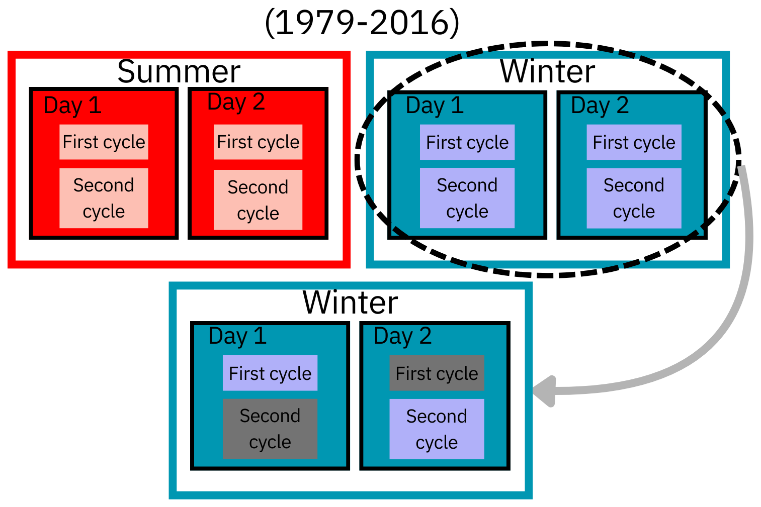
Figure 7 Summary of the database construction: selection of Winter time series and one cycle out of 3.

We now analyze the pair of correlated variables $({\stackrel{\mathrm{̃}}{X}}_M^t,{\stackrel{\mathrm{̃}}{X}}_{M+\mathrm{\Delta }h}^t)$. The autocorrelations and partial autocorrelations (respectively Fig. 3a and b) are not significant for a lag h≥2, which confirms the validity of our hypothesis for an AR(1) model. This is confirmed by the ACF and the PACF of the residuals (see Fig. B1), which show no significant temporal correlations.

We obtain also non significant cross-correlations for the joint vectors $\left(\right({\mathit{\epsilon }}_M^t{)}_{t=\mathrm{1},\mathrm{\dots },\mathrm{37}},\left({\mathit{\epsilon }}_{M+\mathrm{\Delta }h}^t{)}_{t=\mathrm{1},\mathrm{\dots },\mathrm{37}}\right)$, which shows that we comply with the framework assumptions highlighted in Sect. 3.2. Please refer to Appendix B1 for more details. Besides, since we study ${\mathit{\epsilon }}_M^t$'s exceedances for a given t, we assess extremal dependence as defined in Coles et al. (1999). To this end, we apply the statistical test proposed by Thomas (2001) whose null hypothesis is the asymptotic dependence of the residuals ${\mathit{\epsilon }}_M^t$. The null hypothesis is rejected at confidence level 1 % (p value < 10⁻¹⁰), indicating that the residuals ${\mathit{\epsilon }}_M^t$ are asymptotically independent. Then, as detailed in Sect. 3.1.2, we aim at obtaining heavy-tailed marginals for each value of t. To achieve this, following Opitz et al. (2021), we estimate the cdf of ${\mathit{\epsilon }}_M^t$ and apply the transformation 𝒯 to the residuals, obtaining Fréchet marginals $Z_M^t$ for each value of t. An intermediate step involves selecting the threshold parameter u^t used in Eq. (4). To guide this choice, we use the property that for any (w^t>u^t) the exceedances $({\mathit{\epsilon }}_M^t>w^t)$ should follow a GPD law if u^t is a suitable threshold. Accordingly, we define updated parameters $({\mathit{\sigma }}^{\prime },{\mathit{\gamma }}^{\prime })$ that remain stable as w^t increases. With the same objective, we analyze, for each value of t, the behaviour of the mean residual life (MRL) $\mathbb{E}({\mathit{\epsilon }}_M^t-u^t\mid {\mathit{\epsilon }}_M^t>u^t)$ (Coles et al., 2001) as a function of u^t. Guided by these tools, we define u^t as the 90 % percentile of ${\mathit{\epsilon }}_M^t$ since the MRL plot becomes linear beyond this point and the couple $({\mathit{\sigma }}^{\prime },{\mathit{\gamma }}^{\prime })$ remains stable for all thresholds (w^t>u^t) (see Appendix B2). To assess the quality of the marginal transformation, we compare empirical quantiles $Z_M^t$ with those of the Fréchet distribution across various values of t. The levels obtained are close to the theoretical ones, demonstrating the consistency of the transformation. Having marginals $Z_M^t$ with Pareto-type tails is a necessary but not sufficient condition for Z_M to be a regularly varying random element of L²([0,1]), as the latter additionally requires a joint tail condition (see Sect. 2.2.2). As a consequence, we now show that Z_M is regularly varying in the L² sense with index α=1. By Theorem (3.1) of Clémençon et al. (2024), Z_M is a regularly varying random element with index α if and only if Ω_M converges in distribution and the random variable ℓ(Z_M) has a Pareto-type tail with index α. Here, we can be confident that both conditions are satisfied. First, the analysis of the mean projection of Ω_M supports the convergence in law of the angular component (see Appendix C1).

Secondly, using Eq. (1), the transformation induces a change in the tail behavior of the distribution of ℓ(.): while ℓ(ε_M) is light-tailed distributed (see Fig. 8a), ℓ(Z_M) displays a Pareto-type tail with index $\mathit{\alpha }=\mathrm{1}/\mathit{\gamma }\approx \mathrm{1}$ (Fig. 8b), as confirmed by the convergence of the Hill estimator.

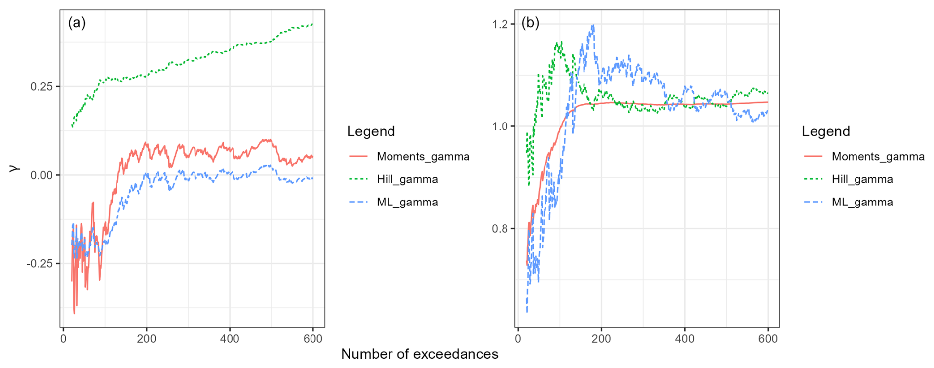
Figure 8 Estimation of γ for: (a) ℓ(ε_M); (b) ℓ(𝒯(ε_M)) (solid line: moments estimator, dotted line: Hill estimator, dashed line: MLE estimator).

5.1.2 Modeling stage based on a polar coordinate representation.

As we get back to the framework assumptions with the pre-processing step, we now choose the threshold u_ℓ that defines the set of extreme observations via the condition ℓ(Z_M)>u_ℓ of Eq. (6). Following Sect. 3.2, the choice of u_ℓ depends on the convergence behavior of Ω_M when u_ℓ goes to infinity. In our case, using the argument detailed in Sect. 5.1.1, Ω_M appears to converge in distribution when the number of extreme observations is between 200 and 300, corresponding to approximately 4 % and 6 % of the database. As a consequence, we select the top 5 % of the dataset, corresponding to approximately 7 extreme observations per year, and represent a sample of the resulting n=259 time series on their original scale and on the Fréchet scale (Fig. 9). The figure shows that applying the marginal transformation amplifies the variations between successive measures.

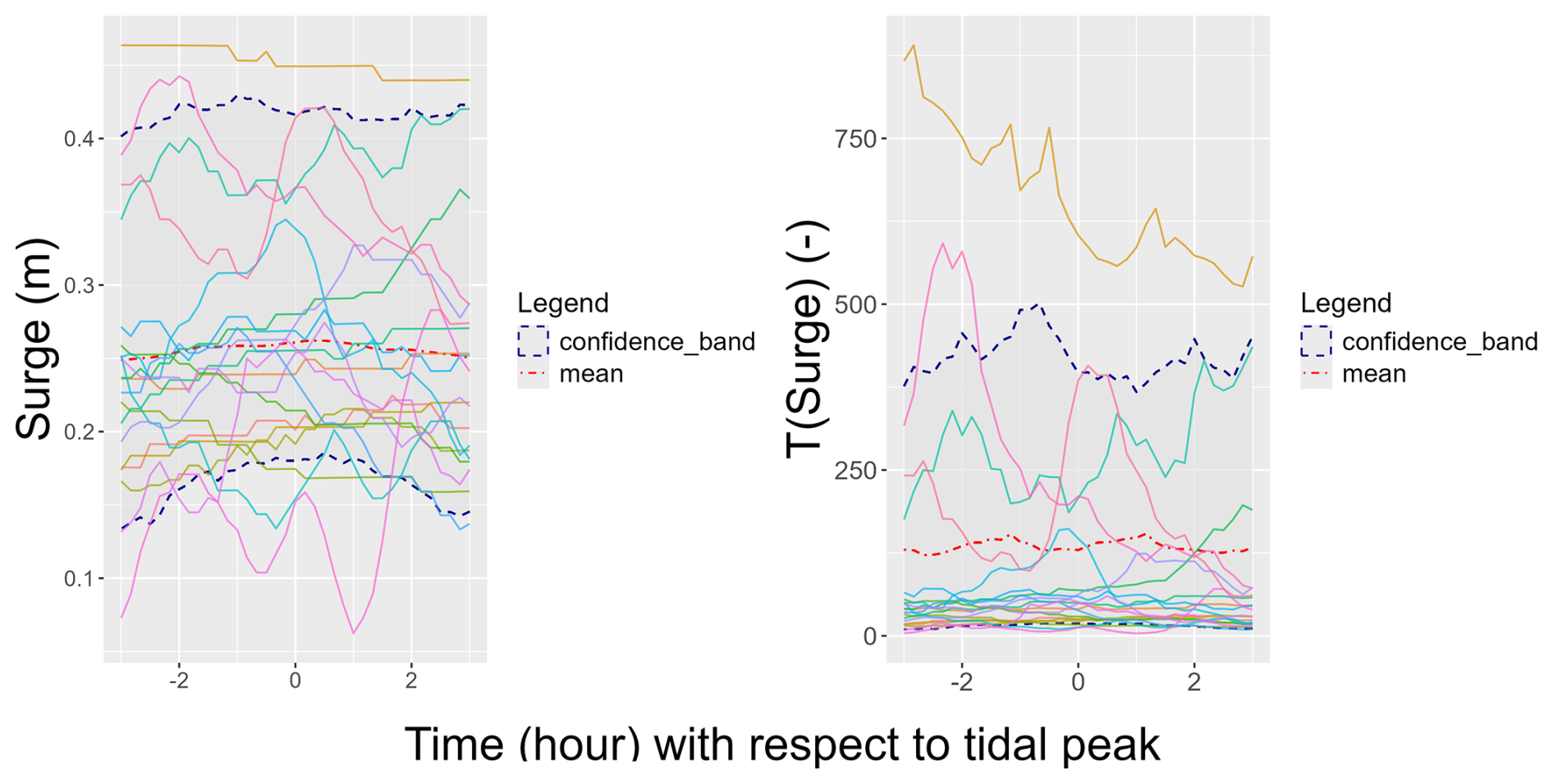
Figure 9 Sample of 20 time series selected for the surge (left panel: original scale, right panel: Fréchet scale with 95 % confidence intervals in dotted lines).

5.2 Backward sense: Simulation of extreme time series

The transformations of the previous section enable us to use a convenient probabilistic model for extreme time series. Following Fig. 6, we now describe the simulator based on this model, which uses the reverse transformations.

5.2.1 Modeling the law of polar coordinates.

We use the polar decomposition defined in Eq. (5) as a basis for our simulation method. After selecting the n=259 extreme observations, we first compute their angular component Ω_M and derive the corresponding PCA basis. Following Sect. 4.1.1, we select the first J=3 eigenvectors of the basis as the ratio (1−R_J) slowly decreases beyond the third dimension (see Appendix C: Fig. C2). With this choice, the selected dimensions explain R_J=83 % of the variance. We use vine copulas and model the joint distribution of the coordinate vector by fitting a range of copula families, namely elliptical and Archimedean copulas such as Tawn and Clayton models, to the bivariate vectors defined by the vine structure. Finally, for each pair of coordinates, we use the Akaike Information Criterion (AIC) (Akaike, 1974) to select the best copula and estimate the tail coefficients $({\mathit{\lambda }}_{+},{\mathit{\lambda }}_{-})$ along with the Kendall's τ. In our case, a t copula is selected for each pair of coordinates. Please refer to Appendix C3 for additional information about the modeling. The iso-density contours of the fitted law are consistent with the distribution of the data points. To go further, as we assume that the observations $(v_{\mathrm{1}},\mathrm{\dots },v_J)$ follow the fitted copula model, we perform some goodness-of-fit tests presented in Schepsmeier (2019). We do not reject the null hypothesis when we use the bootstrap test based on the White statistic (White, 1982) (p value ≈0.5). However, following Caillault and Guegan (2005), using Student copula implies that there is an asymptotic dependence between coordinates. Figure C4 shows that this assumption does not hold for the pair (C₁,C₂). In this case, we can address this issue for the first two coordinates by adopting the second best model, namely the rotated Tawn 1 copula (Cheng et al., 2020), which is well suited for modeling asymptotic independence. In contrast, since the pair (C₂,C₃) exhibits asymptotic dependence, the assumption of the Student copula model remains valid. Using the composite copula model, we simulate new vectors $(v_{\mathrm{sim},\mathrm{1}},v_{\mathrm{sim},\mathrm{2}},v_{\mathrm{sim},\mathrm{3}})$ and transform each coordinate back to its initial scale by applying $F_i^{-\mathrm{1}}$ for $i=\mathrm{1},\mathrm{\dots },\mathrm{3}$. We simulate n_sim=2000 triplets of coordinates from the model and we compare the simulated values with the coordinates of the extreme observations (Fig. 10). The marginals obtained in the simulations are consistent with the data distributions, indicating that our model is consistent with the dependence structure of the coordinate vector.

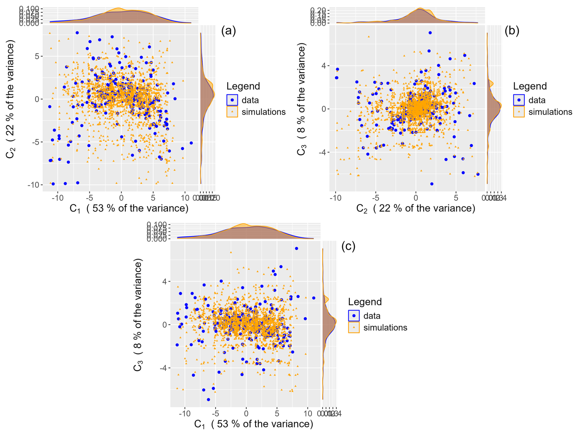
Figure 10 PCA coordinates obtained of 2000 simulated and recorded extreme time series: (a) (C₁,C₂); (b) (C₂,C₃); (c) (C₁,C₃).

We use the coordinates C_sim to obtain the angular components Ω_sim. The resulting patterns resemble that of the extreme observations although the simulated curves appear to be smoother.

5.2.2 Simulating new extreme time series: Applying reverse transformations

Following Sect. 4.2, we generate extreme time series Z_sim by combining the simulated angles Ω_sim with simulations of ℓ(Z_M). Then, we apply the inverse transformation 𝒯⁻¹ to Z_sim to return to the original scale, which produces simulated extreme residuals ε_sim. Using Sect. 4.2.2, we now invert the estimated AR(1) models to return simulated time series ${\stackrel{\mathrm{̃}}{\mathit{X}}}_{\mathrm{sim}}$. We consider two choices of ${\stackrel{\mathrm{̃}}{\mathit{X}}}_{M-\mathrm{\Delta }}$: one observed during the extreme storm Johanna (10 March 2008) and another with a non-extreme behavior (15 February 1986), verifying ℓ(𝒯(ε_M))<u_ℓ. The results, displayed in Fig. 11, show that the choice of ${\stackrel{\mathrm{̃}}{\mathit{X}}}_{M-\mathrm{\Delta }}$ significantly affects both the values and the shape of ${\stackrel{\mathrm{̃}}{\mathit{X}}}_{\mathrm{sim}}$. The left panel reveals notably high values, illustrating the effect of having consecutive extremes.

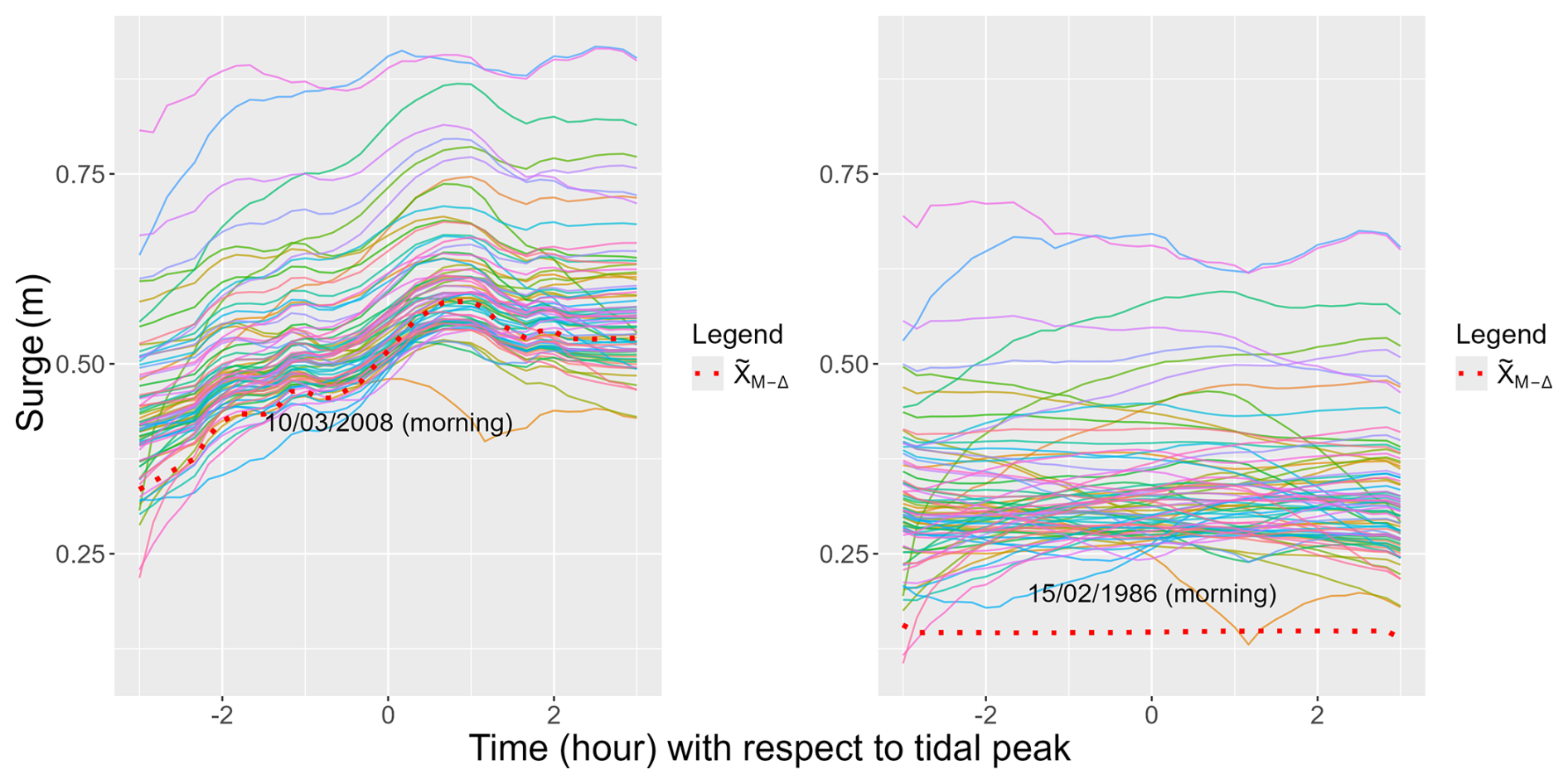
Figure 11 Simulated time series obtained with two different types of ${\stackrel{\mathrm{̃}}{X}}_{M-\mathrm{\Delta }}$ (dotted line) selected among extreme observations (left panel) or non-extreme ones (right panel).

Since the variables (${\stackrel{\mathrm{̃}}{X}}_{M-\mathrm{\Delta }}^t,{\mathit{\epsilon }}_M^t$) are dependent, we apply the conditional sampling illustrated in Sect. 4.2.2 (see Appendix C4). Then, we generate new time series ${\stackrel{\mathrm{̃}}{\mathit{X}}}_{\mathrm{sim}}$ by using ε_sim and the selected ${\stackrel{\mathrm{̃}}{\mathit{X}}}_{M-\mathrm{\Delta }}$ (see Fig. 12). We see that the shape and the values of simulated and observed extreme time series are quite similar, suggesting that our simulations are consistent with the observations. However, we can use other methods to validate our simulator, which is discussed in detail in the following.

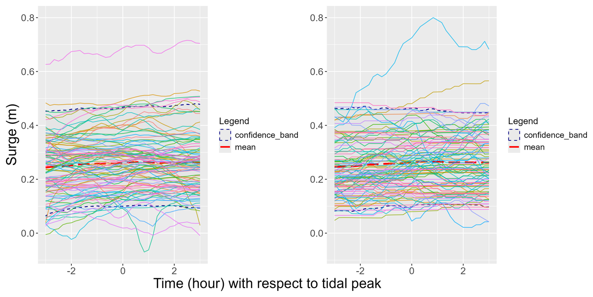
Figure 12 Comparing simulated time series and extreme observations. Left panel: simulated sample of 100 extreme time series, right panel: sample of 100 extreme observations. The dotted lines represent the 95 % confidence bands.

5.3 Consistency of simulations with extreme observed time series

We validate our simulator by comparing simulated time series with extreme observations. To this end, we use a set of diagnostic tools, using extreme value analysis (Coles et al., 2001), PCA and classification algorithms.

5.3.1 Comparison of percentile levels

First, we compare the empirical percentiles at each time point t with those derived from the simulated time series (Fig. 13). To quantify uncertainty in the observations, we construct a bootstrap 95 % confidence band by resampling the extreme time series 500 times. The simulated levels obtained are coherent with the observations as the simulations' percentiles lie within the data confidence band.

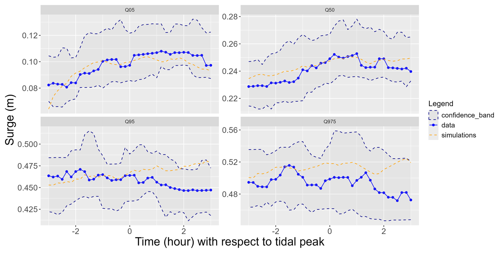
Figure 13 Percentiles obtained in the data and in the simulations (blue lines: data, orange dotted lines: simulations).

5.3.2 Comparison of coordinates in a PCA basis

The simulated extreme time series should exhibit shape similarities with the observed extremes. One simple way to compare the shape of the time series is to use dimensionality reduction methods and to compare the resulting coordinates. To this end, we analyse the angles of the time series as the simulations extrapolate the L² norm of the observations. We apply PCA to the time series $\stackrel{\mathrm{̃}}{\mathit{X}}/\mathrm{\ell }\left(\stackrel{\mathrm{̃}}{\mathit{X}}\right)$ and, to preserve potential differences, both simulated and observed series are further normalized by using the mean and the standard deviation of the observations. Then, we compare the PCA coordinates of recorded time series with those of simulated time series (Fig. 14). The similarity in the score distributions suggests that simulated time series and extreme observations exhibit comparable behavior. Yet, this similarity is more pronounced in the first dimension, which accounts for the largest proportion of variability (here 60 %). A KS test confirms that simulations' and observations' coordinates follow the same law in the first dimension (p value ≈27 %) but do not in the second dimension (p value $\approx \mathrm{7.7}\times {\mathrm{10}}^{-\mathrm{5}}$).

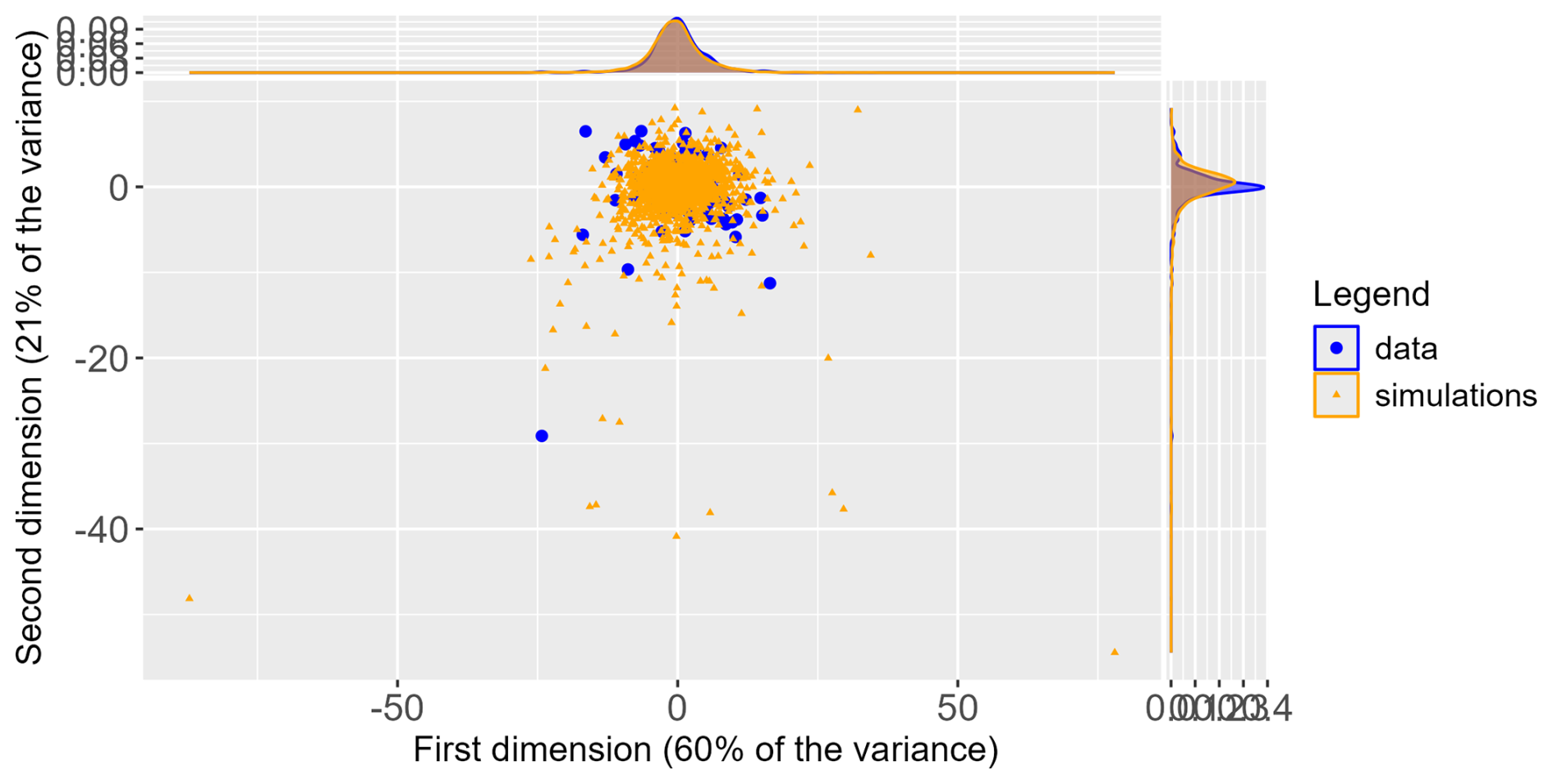
Figure 14 PCA coordinates for S in simulations (orange triangles) and extreme observations (blue dots).

5.3.3 Comparison of the distribution upper tails.

Then, we compare the temporal dependence within each tidal cycle between observations and simulations, with a focus on extremal dependence. Following (Opitz et al., 2021; Dell'Oro and Gaetan, 2025), we assume that ${\stackrel{\mathrm{̃}}{X}}_M^t$ and ${\stackrel{\mathrm{̃}}{X}}_M^s$ are asymptotically dependent for all pairs (t,s). To quantify the dependence, we estimate the ℓ-extremogram (de Fondeville and Davison, 2022) for both the recorded and simulated time series. We detail the approach in Appendix D1. We focus on the values exceeding the 90 % percentile and use 500 resamples to construct a bootstrap 95 % confidence band. The extremogram of the simulated time series lies within the confidence band (Fig. 15) based on the observed extreme time series.

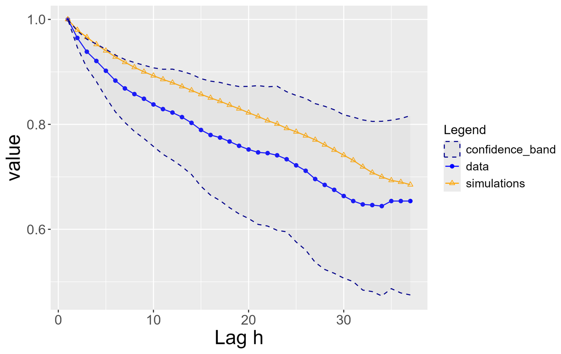
Figure 15 Extremogram for S for simulations (orange) and observations (blue) with confidence bands in dotted lines.

Moreover, the density obtained at each time t should be an extrapolation of the observed data. Directly using the quantiles of the simulations may produce very large values. This occurs because we simulate ${\stackrel{\mathrm{̃}}{X}}_{\mathrm{sim}}$ verifying ℓ(𝒯(ε_M))>u_ℓ, meaning their extremes can be larger than those observed. In this setting, we compare our values with the empirical quantiles of the observations and the fitted law of exceedances. Following Solari et al. (2017), the results are expressed in terms of return period P and corresponding return levels, with approximately 7 extreme observations per year (Fig. 16). All implementation details are provided in Appendix D2. The highest simulated levels fall within the confidence band, indicating that our simulations look similar to the extreme observations. Thus, they can be considered a reliable extrapolation of the observed data toward higher values.

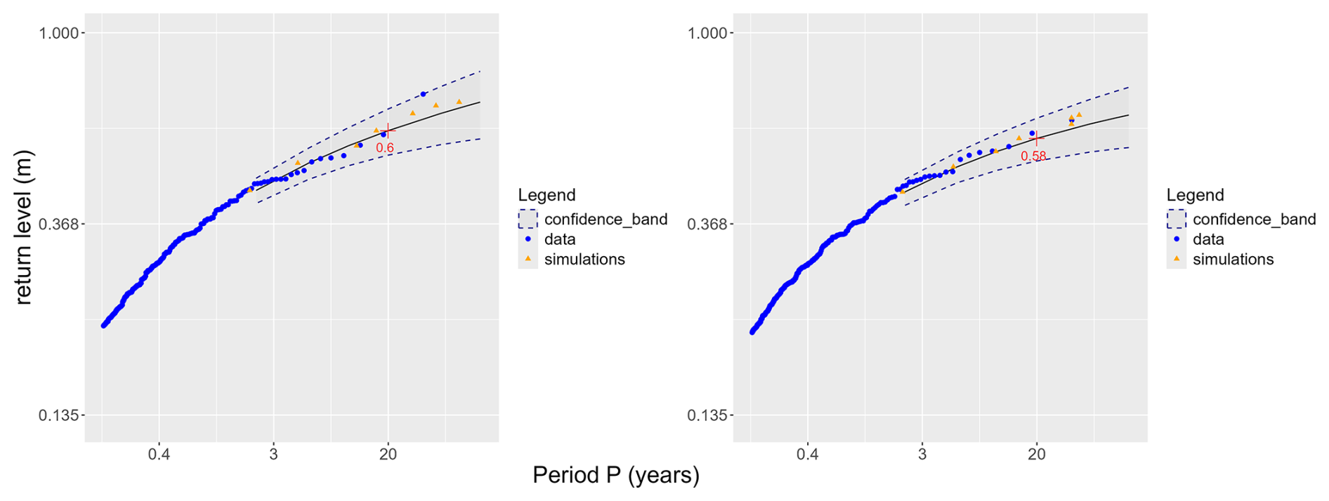
Figure 16 Return level for simulations (orange triangles) and observations (blue dots), for two different values of t. Left panel: t=19 (tidal peak), right panel: t=13 (one hour before). The dotted lines represent 95 % confidence bands.

5.3.4 Comparison of predictions with classification algorithms.

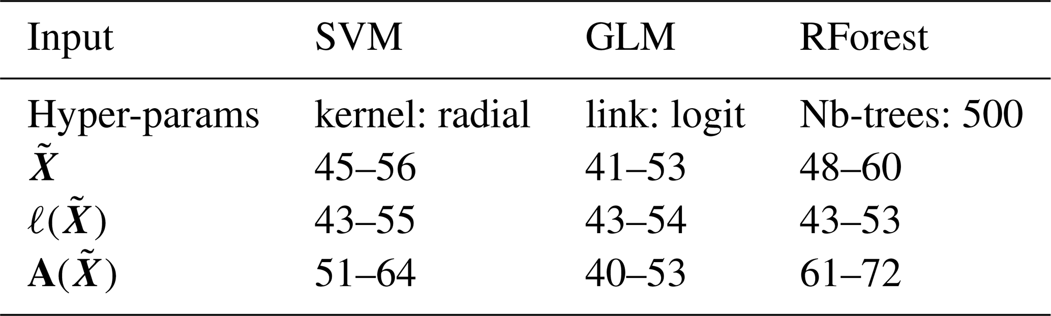
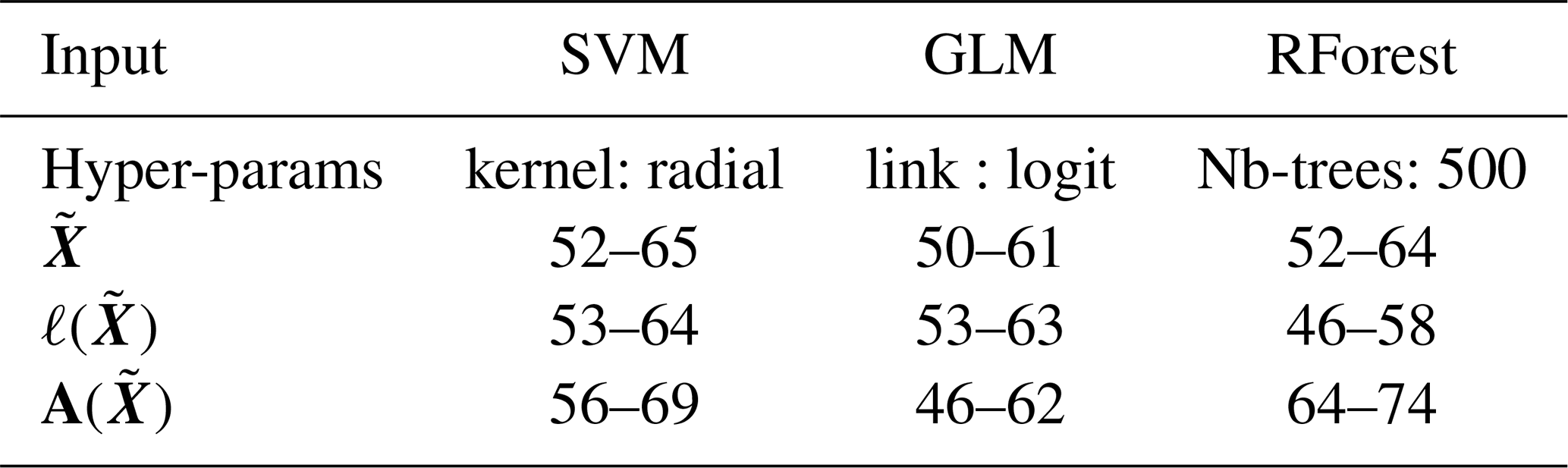
Finally, following the same idea as two-sample classification tests (Lopez-Paz and Oquab, 2016; Watson et al., 2023), we rely on a classification-based approach to determine whether the generated extreme time series differ from the original dataset. We define a binary classification problem, where the target variable y equals 1 if the input x is a simulated time series, 0 otherwise. The goal is to learn a function g that, given the input x, predicts the correct class y. If the simulations behave like the extreme observations, such classifier should hardly identify the simulated time series, resulting in an accuracy close to 50 %. To address this question, we begin by randomly drawing n=259 simulated time series without replacement (Step 1) since the number of simulated time series n_sim=2000 differs from n. We construct a dataset composed of these sampled time series and extreme observations, ensuring that simulated time series make up 50 % of the data. Then, after splitting this dataset into training and testing subsets, we train our model on the training part (Step 2). Finally, we evaluate the model's overall accuracy on the test set (Step 3). To account for the influence of the sampling used in Step 1, we repeat 100 times these three steps and provide a confidence interval of order 90 % for the overall accuracy. We use three classifiers with this approach: a support-vector machine (SVM) with a radial kernel, a generalized linear model (GLM), and a random forest (Hastie et al., 2009). We apply this procedure with different types of input features: the time series, its norm and its angle. If we provide the time series, all classifiers achieve an overall accuracy close to 50 % (see Table 1), meaning that the ML models struggle to identify simulated time series. This suggests that our simulations are quite consistent with the observed data. For example, the distributions of $\mathrm{\ell }\left({\stackrel{\mathrm{̃}}{\mathit{X}}}_{\mathrm{sim}}\right)$ and $\mathrm{\ell }\left({\stackrel{\mathrm{̃}}{\mathit{X}}}_M\right)$ are quite similar (see Appendix D4), with differences appearing for the largest values as the simulations better explore the extremes of $\mathrm{\ell }\left({\stackrel{\mathrm{̃}}{\mathit{X}}}_M\right)$. In contrast, when using the angle as input feature, the models are better able to distinguish between simulations and observations but the accuracy still remains low on the order of 60 % in average.

Table 1 Confidence intervals at order 90 % for the global accuracy.

This approach also reveals the influence of ${\stackrel{\mathrm{̃}}{\mathit{X}}}_{M-\mathrm{\Delta }}$ as the attained accuracy depends on the sampling method, which is discussed in Appendix E. The classifiers identify more easily the simulated time series when an unconditional sampling is used. For instance, the overall accuracy exceeds 50 % when the time series itself is used as input.

6 Conclusion

Motivated by the modeling of surge-induced coastal flooding, our goal is to develop a simulator for extreme time series. To this end, we align our time series with the framework of regular variations. As the observations do not meet standard assumptions, we get back to the framework setting by applying an autoregressive model and marginal transformation to the time series. It allows us to obtain a probabilistic model and to develop a simulation method capable of simulating data-like extreme time series, following the same law as extreme observations, but also consecutive extremes.

We apply this method to a hindcast database (Idier et al., 2020) from the site of Gâvres in Brittany, which is considered as a set of observations in our developments. To evaluate the quality of our simulations, we provide several approaches, including a classification task where the goal is to distinguish between observed and simulated time series. Our results support the validity of our simulation approach as machine learning algorithms struggle to reliably distinguish the two groups.

We rely on dimension reduction and parametric copula models to simulate new extreme time series. However, alternatives approaches can be considered to model the distribution of the angular component without departing from the proposed framework, such as Gaussian mixture (Nanty et al., 2017) or generative deep learning approaches (Wessel et al., 2025). Moreover, although this paper focuses on simulating univariate extreme time series, real-world forcing conditions evolve in a multivariate context (Rohmer et al., 2022; Gouldby et al., 2014) as other variables such as wind speed also intervene at each time step. Therefore, extending the approach to the multivariate case (Kim and Kokoszka, 2024) represents a promising direction for effectively modeling extreme forcing conditions.

Appendix A: Complements on data analysis

A1 Cross-correlations

Figure A1 shows that there are several significant correlation peaks for the pair $(X_M^t,X_{M+h}^{t^{\prime }})$ with t=1, $t^{\prime }=\mathrm{2}$. As a consequence, the joint vectors $\left(\right(X_M^t{)}_{t=\mathrm{1},\mathrm{\dots },\mathrm{37}},\left(X_{M+h}^t{)}_{t=\mathrm{1},\mathrm{\dots },\mathrm{37}}\right)$ are not independent.

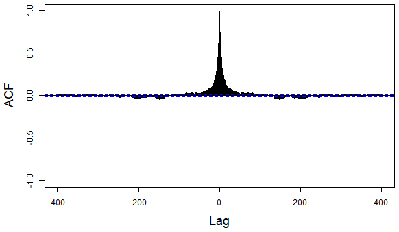
Figure A1 ACF for the pair $(X_M^{\mathrm{1}},X_{M+h}^{\mathrm{2}})$. The peak at lag h=0 corresponds to the correlation between the measures observed during the same tidal cycle.

A2 Seasonality

We present here the evolution of the surge at tidal peak, t=19, according to the month considered (Fig. A2). The extremes of Winter values are much higher than the extremes of summer values, which is explained by a higher frequency of storms in Winter.

Figure A2 Seasonal evolution of the distribution of the surge at tidal peak.

Appendix B: Whitening and marginal transformation

B1 Effect of the autoregressive models

We present here the effect of applying the autoregressive models on ${\stackrel{\mathrm{̃}}{X}}_M^t$. We can first use the ACF and the PACF on the residuals ε_M (Fig. B1).

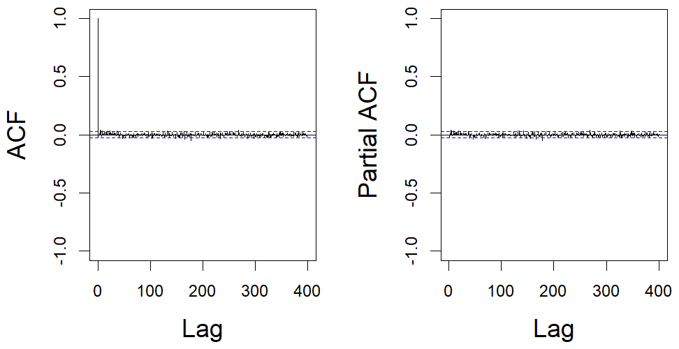
Figure B1 Pearson's correlations observed for S at t=19. Left panel: ACF, right panel: PACF. The dotted blue lines correspond to the confidence interval in case of a Gaussian white noise.

Besides, since we aim at retrieving the assumptions of the framework, we analyse the cross-correlations of the joint vectors $\left(\right({\mathit{\epsilon }}_M^t{)}_{t=\mathrm{1},\mathrm{\dots },\mathrm{37}},\left({\mathit{\epsilon }}_{M+\mathrm{\Delta }h}^t{)}_{t=\mathrm{1},\mathrm{\dots },\mathrm{37}}\right)$. Figure B2 shows that we obtain for instance non significant correlations for the pair $({\mathit{\epsilon }}_M^{\mathrm{1}},{\mathit{\epsilon }}_{M+\mathrm{\Delta }h}^{\mathrm{2}})$.

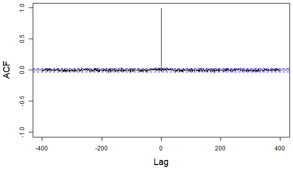
Figure B2 ACF for the pair $({\mathit{\epsilon }}_M^{\mathrm{1}},{\mathit{\epsilon }}_{M+\mathrm{\Delta }h}^{\mathrm{2}})$. The peak at lag h=0 corresponds to the correlation between the measures observed during the same tidal cycle.

Correlations of extremes

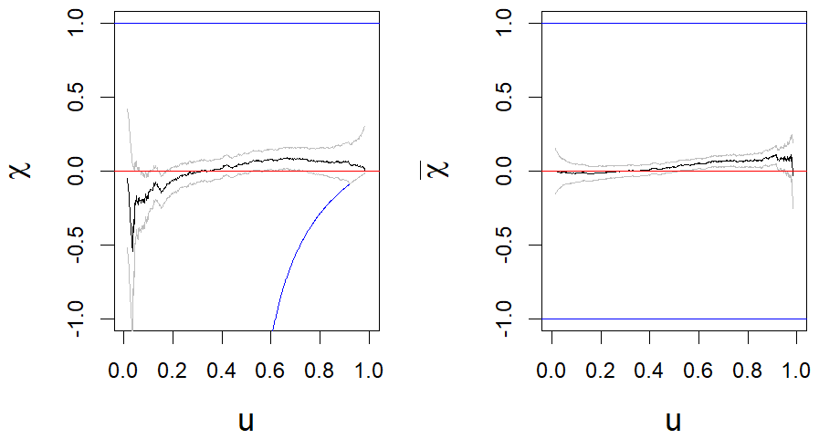
Figure B3 Measures of asymptotic dependence for the surge for (t=19, h=1) with confidence band (grey lines). The blue lines represent the theoretical bounds of the correlation coefficient.

Figure B4 Graphic diagnostics for the residual of S at tidal peak (t=19).

We recall the definition of the χ measure (Coles et al., 2001). Let U and V be two variables with uniform distributions and we note $\mathit{\chi }\left(u\right)=\mathbb{P}(V>u\mid U>u)$ with $(\mathrm{0}<u<\mathrm{1})$. They are asymptotically independent if χ(u)→0 when u→1. In this case, $\stackrel{\mathrm{‾}}{\mathit{\chi }}$ measures the dependence between the two variables. In our case, the pair (U,V) corresponds for a given t and h to the pair (${\mathit{\epsilon }}_M^t,{\mathit{\epsilon }}_{M+\mathrm{\Delta }h}^t$) after a rank transformation. At the tidal peak (t=19), 0 belong to the confidence interval of χ(u) when u>0.9 for h=1 (Fig. B3). As a consequence, we cannot reject the hypothesis of asymptotic independence.

B2 Marginal transformation

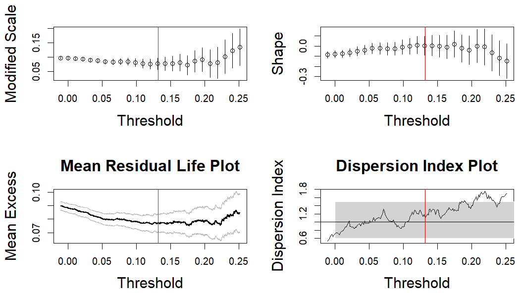
We describe the evolution of diagnostic statistics when u^t is between the median of ${\mathit{\epsilon }}_M^t$ and its 98 % quantile. We observe the evolution of the MRL and the updated parameter (Fig. B4). We represent with the red line the threshold chosen for the marginal transformation. We do have a stable couple (${\mathit{\sigma }}^{\prime },{\mathit{\gamma }}^{\prime }$) (top left and top right) and the MRL (lower left corner) seems to be a linear function.

We show the evolution of the dispersion index in the lower right corner. This tool is based on the link between extreme values and Poisson point process. u^t is a consistent threshold if the index is around 1, which is the case for the threshold we chose.

Appendix C: Complements on the simulation of extreme time series

C1 Choice of the extreme individuals

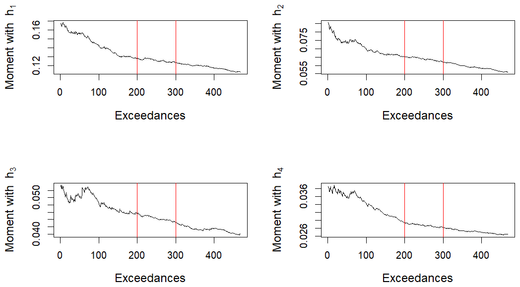
The convergence of Ω_M is closely related to the stability of GPD parameters (Sect. 5.1.1) as we seek a convergence regime of $\mathbb{E}\left(\right|\langle {\mathbf{\Omega }}_M,h_j\rangle \left|\right)$. Here, we take h_j(t)=sin (2πjt) with $j\in \mathit{\{}\mathrm{1},\mathrm{\dots },\mathrm{8}\mathit{\}}$. We examine the evolution of the mean of $|\langle \mathit{f}/\mathrm{\ell }(\mathit{f}),h_j\rangle |\mid \mathrm{\ell }\left(\mathit{f}\right)>u_{\mathrm{\ell }}$ as the threshold u_ℓ increases. Figure C1 shows that there is a stability region for the mean projection across several functions when the number of extreme time series lies between 200 and 300.

Figure C1 Evolution of the mean projection for Ω_M.

C2 Choice of the number J

As we increase the number J used in the truncated expression of Ω_M, we analyze the evolution 1−R_J (Fig. C2).

Figure C2 Evolution of the unexplained inertia of Ω_M for S.

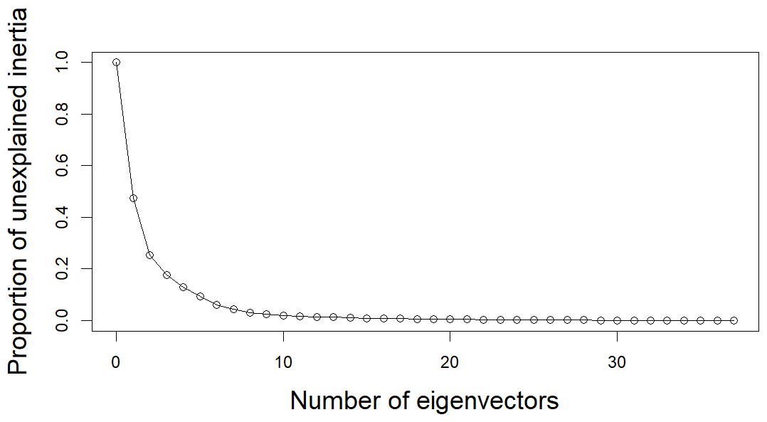
After choosing J=3, we simulate n_sim=2000 angles and compare our simulations with the angles of the extreme observations (Fig. C3).

Figure C3 Comparison of the angles Ω_M (left panel) and Ω_sim for S (right panel).

C3 Details on the copula family

We describe here the parameters estimated for the copula (Table C1).

Table C1 Modeling of Ω_M's coordinates with copulas: the first row explains the modeling of the law of the first two coordinates while the last one presents the modeling of the conditional law of (C₁,C₃) knowing C₂.

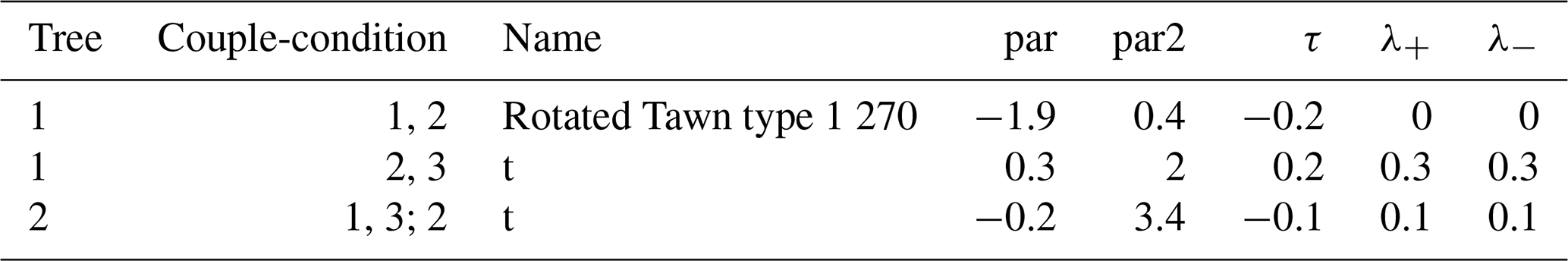
As detailed in Sect. 5.2.1, although the t copula is selected as the best model for the pair (C₁,C₂) according to the BIC and AIC criteria, this pair exhibits asymptotic independence (Fig. C4). We therefore adopt the second-best model instead. We compare the fitted copula models with observed coordinates by looking at the relationship between the two dimensions. In Figs. C5 and C6, we compare the data observations with the iso-density curves of the model respectively in the uniform scale and in the data scale. Figure C5 shows that we are able to capture the most of the dependence structure as the distribution of data points is coherent with the levels found. However, if we return to the original scale of the coordinates, we see on Fig. C6 the limits of our modeling as some data points do not coincide with the iso-density curves of our model.

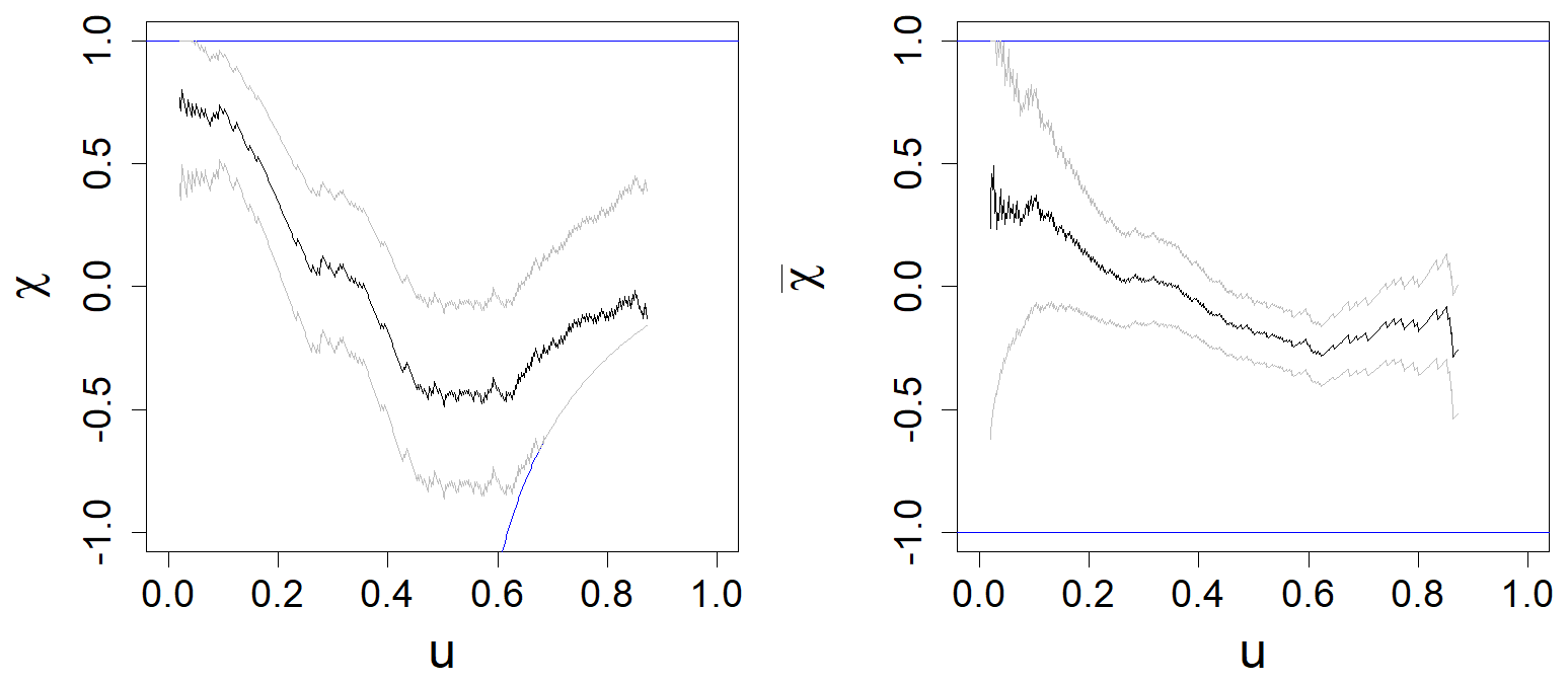
Figure C4 Measures of asymptotic dependence for the pair (C₁,C₂) with confidence band (grey lines). The blue lines represent the theoretical bounds of the correlation coefficient.

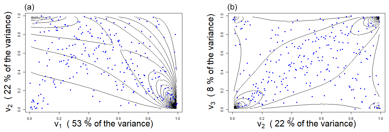
Figure C5 Iso-density curves (dark lines) of the copula with the data coordinates (blue points): (a) (v₁,v₂), (b) (v₂,v₃).

We also use statistical tests to compare our model with the law of the observations. The null hypothesis H₀ is that the observations follow the model. We reject H₀ if we apply the White test under the asymptotic distribution of the test statistic (p value ≈0.2 %). However, when using the bootstrapped distribution, we do not reject the null hypothesis, which is consistent with the result of the Kolmogorov–Smirnov (KS) test on the empirical copula process.

C4 Choice of ${\stackrel{\mathrm{̃}}{\mathit{X}}}_{M-\mathrm{\Delta }}$

We apply a conditional sampling of ${\stackrel{\mathrm{̃}}{\mathit{X}}}_{M-\mathrm{\Delta }}$ knowing ε_sim. The resulting levels are quite coherent with those observed in the dataset (Fig. C7) and simulations provide as expected fill gaps where data observations are not available.

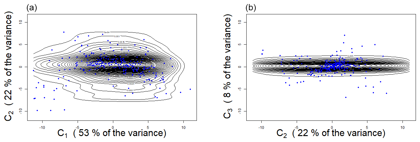
Figure C6 Iso-density curves (dark lines) of the joint law with the data coordinates (blue points): (a) (C₁,C₂), (b) (C₂,C₃).

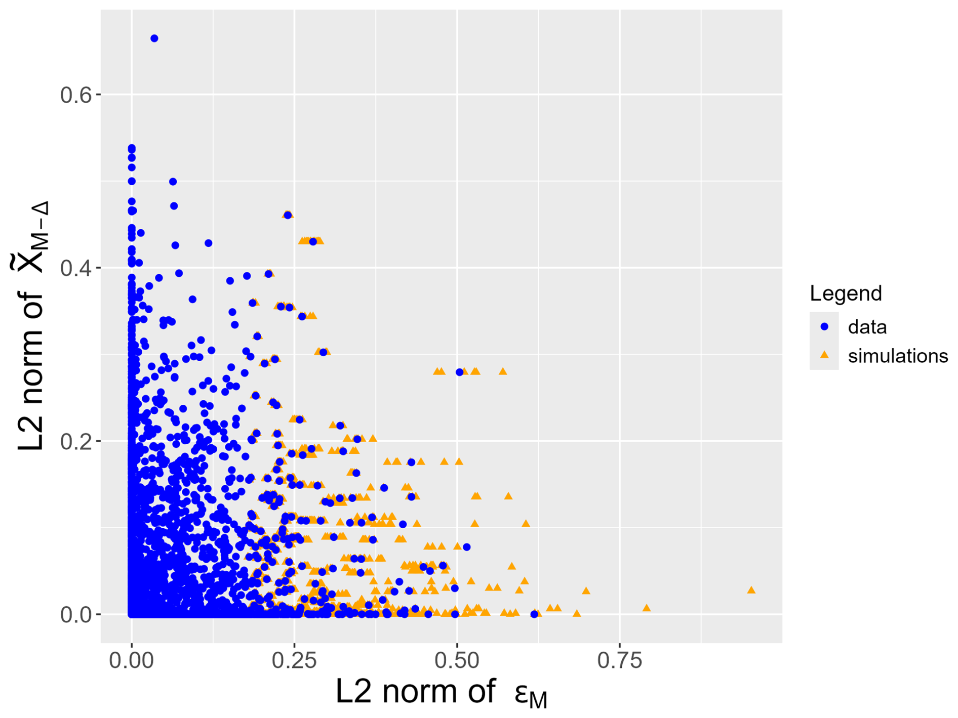
Figure C7 Relation between for S (blue dots: data points, orange triangles: coordinates obtained in the simulations).

Appendix D: Complements on the consistency of simulations with the observations

D1 Correlation of extremes

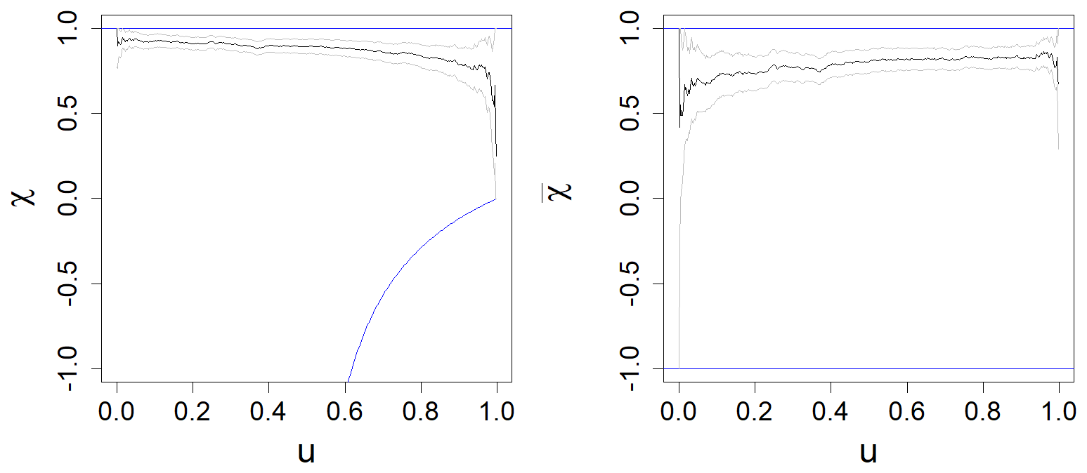
Figure D1 Measures of asymptotic dependence between ${\stackrel{\mathrm{̃}}{X}}_M^{\mathrm{1}}$ and ${\stackrel{\mathrm{̃}}{X}}_M^{\mathrm{37}}$ for the surge with confidence band (grey lines). The blue lines represent the theoretical bounds of the correlation coefficient.

The extremogram is defined for extreme time series with

$$\begin{array}{}\text{(D1)}& \mathit{\pi }(s^{\prime },s)={\lim }_{q\to \mathrm{1}}\mathbb{P}({\stackrel{\mathrm{̃}}{X}}_M^{s^{\prime }}>u_q(s^{\prime })\mid {\stackrel{\mathrm{̃}}{X}}_M^s>u_q(s\left)\right),\end{array}$$

where $u_q\left(s\right)=F_s^{-\mathrm{1}}\left(q\right)$ is the quantile function of order q of ${\stackrel{\mathrm{̃}}{X}}_M^s$. We use q=0.9 to compare our simulations with the extreme time series. This tool is based on the hypothesis of asymptotic dependence between the values of the same tidal cycle. We can see for example that the first and the last value of a time series are asymptotically dependent (Fig. D1) as χ does not converge to 0 when u goes to 1.

D2 Return level estimation

To obtain the levels obtained in the simulations, we use the formula

$$\begin{array}{}\text{(D2)}& \mathbb{P}(A\mid B)=\mathbb{P}(A\mid B,C)\mathbb{P}(C\mid B)+\mathbb{P}(A\cap \stackrel{\mathrm{‾}}{C}\mid B),\end{array}$$

with $A=({\stackrel{\mathrm{̃}}{X}}_M^t\le x)$, $B=({\stackrel{\mathrm{̃}}{X}}_M^t>u^t)$ and $C=\left(\mathrm{\ell }\right(\mathcal{T}\left({\mathit{\epsilon }}_M\right))>u_{\mathrm{\ell }})$. The first member on the right-hand side is directly estimated in the simulated time series whereas we use observations to estimate other members. Then, we use the model quantiles as x levels. The probability $p=\mathbb{P}(A\mid B)$ is associated to a return period. The link between the quantile order p and the return period P is given by the formula

$$\begin{array}{}\text{(D3)}& P={\displaystyle \frac{\mathrm{1}}{\mathrm{npy}(\mathrm{1}-p)}},\end{array}$$

where npy is the average number of extreme observations per year, chosen at 7 events per year. Thus, looking at Fig. 16 (left panel), if we observe one day a surge of 0.6 m at tidal peak (t=19 for every cycle), we will wait in average 20 years before seeing an event reaching this extreme level.

D3 Extreme aspects

We can analyze the extreme values obtained for other values of t in the simulations and in the data (Fig. D2). The levels obtained are consistent with the theoretical values.

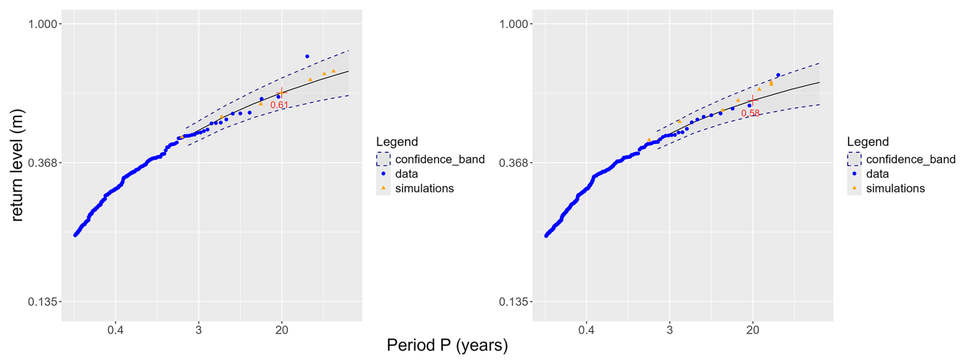
Figure D2 Return level for simulations (orange triangles) and observations (blue dots), for two different values of t. Left panel: t=25 (one hour after the tidal peak), right panel: t=31 (two hours after the peak). The dotted lines represent 95 % confidence bands.

D4 Distribution of ℓ(.) for simulated and observed extreme time series

We describe here what we obtain for the ℓ(.) function in the simulations and in the extreme time series (Fig. D3). The shape of the two distributions are quite similar but their extreme values are quite different. While the maximum value in the data is slightly above 0.6 m, the maximum value obtained in the simulation is larger than 0.8 m.

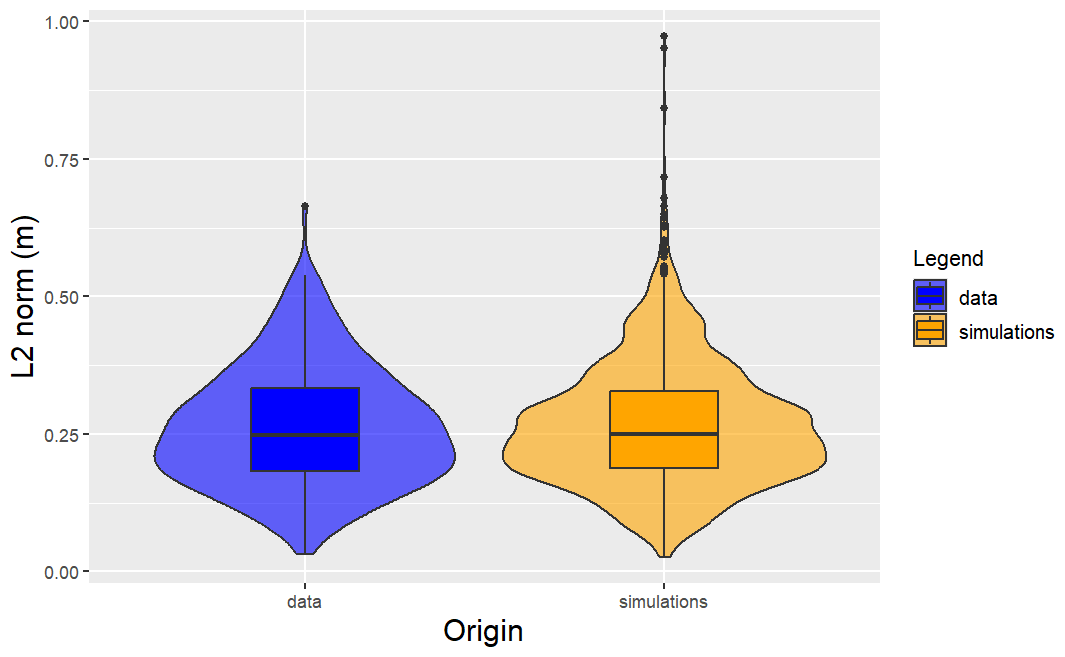
Figure D3 Distribution of ℓ(S) (orange: simulated time series, blue: recorded extreme time series).

Appendix E: Choice of ${\stackrel{\mathrm{̃}}{\mathit{X}}}_{M-\mathrm{\Delta }}$

Here, we present the effect of using an unconditional sampling of ${\stackrel{\mathrm{̃}}{\mathit{X}}}_{M-\mathrm{\Delta }}$.

E1 Comparison of percentile levels

Firstly, we analyze the quantiles obtained for each value of t in the simulated time series and in the extreme observations (Fig. E1). We see that for several orders the quantile obtained in the simulations do not belong to the confidence interval of the extreme observations.

E2 Comparison of coordinates in a PCA basis

We use the PCA decomposition of the angle ${\stackrel{\mathrm{̃}}{\mathit{X}}}_M/\mathrm{\ell }\left({\stackrel{\mathrm{̃}}{\mathit{X}}}_M\right)$ of the extreme observations with the unconditional sampling of ${\stackrel{\mathrm{̃}}{\mathit{X}}}_{M-\mathrm{\Delta }}$. Figure E2 shows that the quantiles of simulated coordinates do not behave like the observed coordinates as empirical quantiles are deviating from the bisector. As a consequence, the observations' and simulations' coordinates do not follow the same law for the first dimension with a p value of $\mathrm{6.6}\times {\mathrm{10}}^{-\mathrm{5}}$ for the KS test.

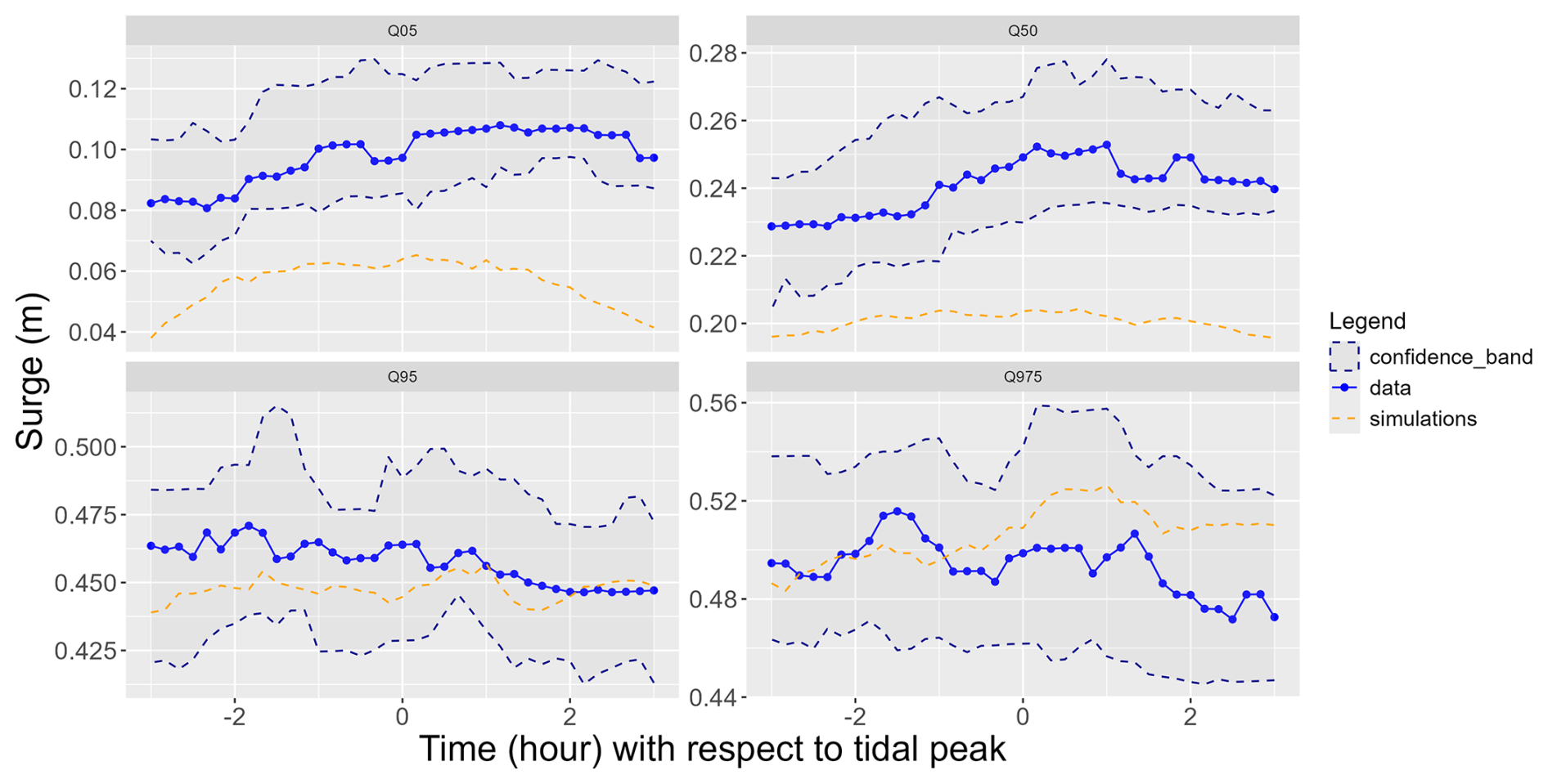
Figure E1 Percentiles obtained in the data and in the simulations without the conditional sampling (blue lines: data, orange dotted lines: simulations).

E3 Comparison of the distribution upper tails

We compare the behaviour of extreme values for the simulated and recorded extreme time series when unconditional sampling is used. We see for instance that the ℓ-extremogram estimated in the simulations is further from the data estimation with conditional sampling than what we obtain with conditional sampling (Fig. E3). Consequently, the selection method does have an impact on the result.

Table E1 Confidence intervals at order 90 % for the global accuracy.

E4 Comparison of predictions with classification algorithms

We focus on the performances of the classifiers (Table E1). The models are able to identify the simulated time series as 50 % does not belong to the confidence interval.

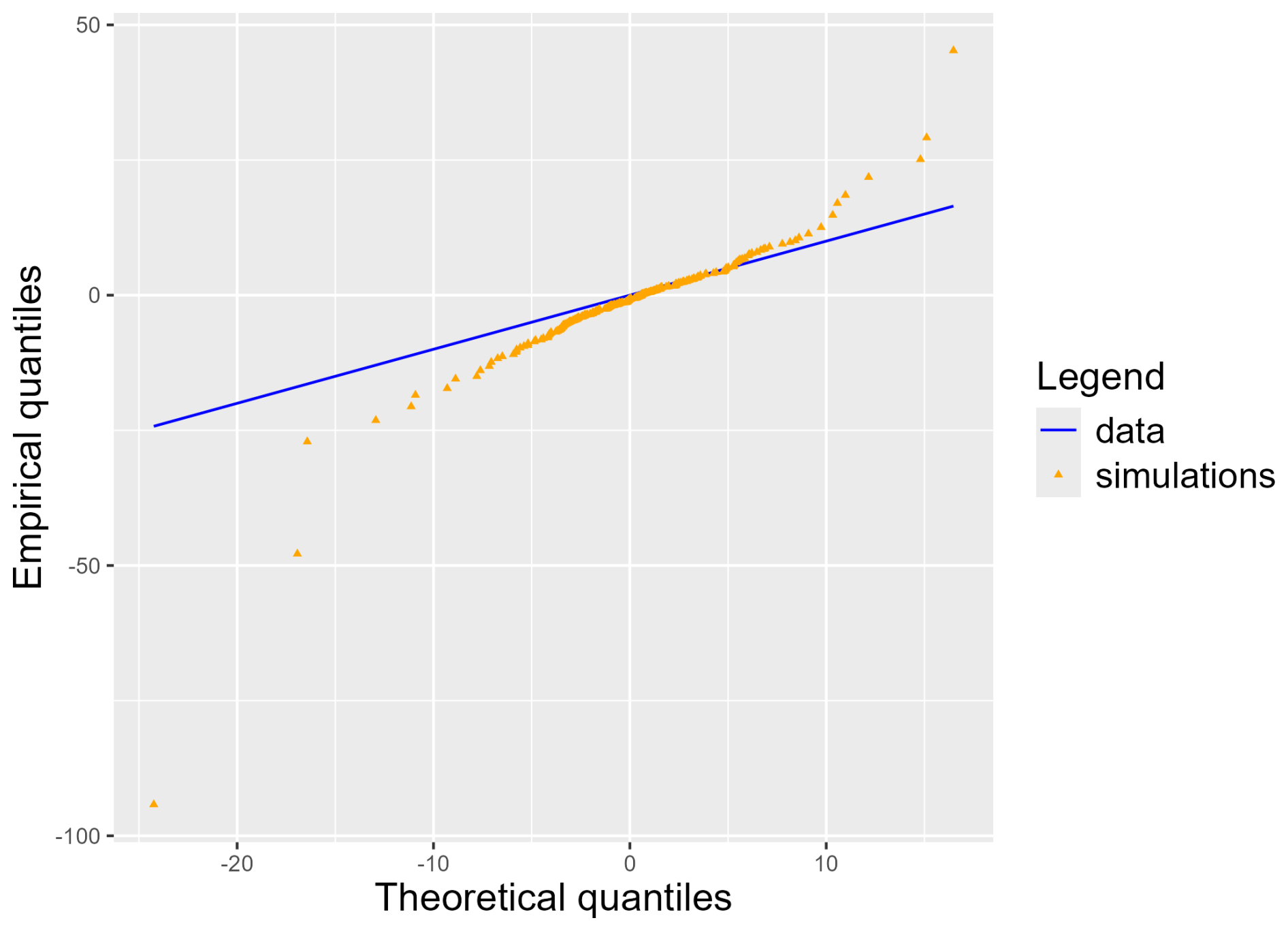
Figure E2 Q–Q plot for C_sim,1 (orange triangles) on data scale (blue line) with the unconditional sampling of ${\stackrel{\mathrm{̃}}{\mathit{X}}}_{M-\mathrm{\Delta }}$.

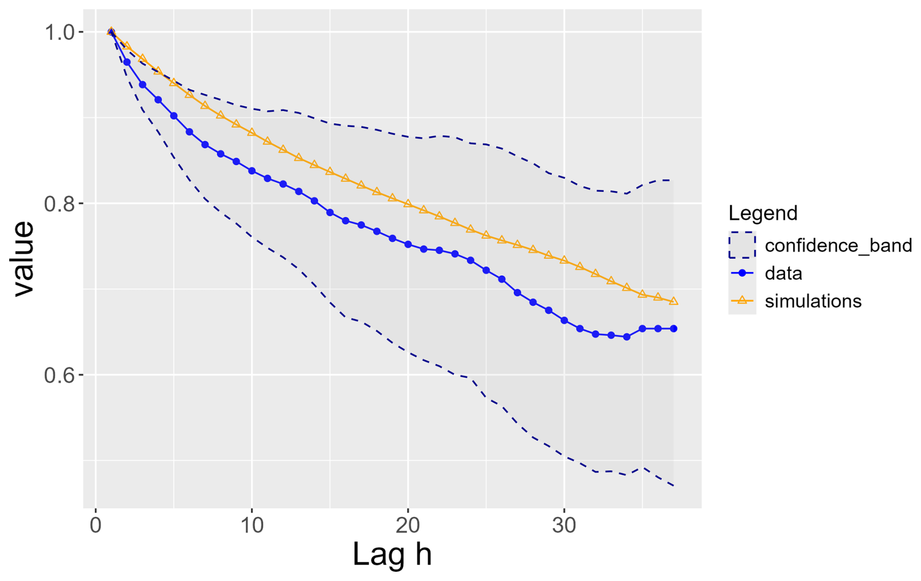
Figure E3 Extremogram for S for simulations (orange) and observations (blue) with confidence bands in dotted lines. Values obtained with the unconditional sampling.