Selecting the best distribution for modeling trends in low, medium, and extreme daily precipitation under climate change

Changes in mean precipitation and the frequency and intensity of extreme precipitation represent one of the most consequential aspects of anthropogenic climate change. This study evaluates a set of statistical distributions for modeling trends across the full precipitation spectrum (low, medium, and extreme daily quantiles). Modeling with a single flexible distribution ensures statistical consistency, thereby avoiding the artificial separation and discontinuity inherent in multi-model approaches. We used time as a covariate for dry-day frequency and sea surface temperature for the wet-day distribution parameters. We applied the methodology to a dense network of over 900 meteorological stations in France, offering a wide variety of climatic regimes, allowing for a robust conclusion. We employed a multi-criterion approach to select the best model, in the first step using the Akaike Information Criterion, and then based on their ability to flexibly capture trends across low, medium, and extreme precipitation quantiles. Our findings highlight that three-parameter distributions (generalized gamma and extended generalized Pareto distribution), particularly with evolving shape parameters, are essential for accurately capturing observed differential changes across the full precipitation spectrum, a flexibility that the two-parameter gamma distribution notably lacked. Although AIC generally favored generalized gamma, both generalized gamma and the extended generalized Pareto distribution demonstrated robust performance. This research underscores the critical need for a multi-criterion model identification framework in nonstationary trend analysis to provide reliable insights essential for hydrological and climate impact assessments.

1 Introduction

Changes in precipitation patterns, particularly in the frequency and intensity of both mean and extreme events, represent one of the most consequential aspects of anthropogenic climate change (IPCC, 2023). Detecting and modeling such changes are critical for improving hydrological forecasting, assessing flood and drought risks, and informing infrastructure planning and climate adaptation strategies.

Accurately assessing these trends requires robust statistical models that can capture the complex behavior of daily precipitation. Daily precipitation poses well-known statistical challenges. It is non-negative, skewed, exhibits a discrete-continuous nature with periods of no rainfall (dry-days) interspersed with varying intensities of rainfall (wet-day), and often shows heavy tails (Papalexiou and Koutsoyiannis, 2013; Cavanaugh et al., 2015). Traditional statistical approaches often simplify this complexity, either by focusing solely on trends in mean precipitation (e.g. Ménégoz et al., 2020), or by treating only extreme events using nonparametric approaches (e.g. Bauer and Scherrer, 2024) or parametric techniques based on Generalized Extreme Value (GEV) distribution (e.g. Blanchet et al., 2021a; Blanchet and Creutin, 2022), or generalized Pareto (GPD) (e.g. Tramblay et al., 2013). However, in applications such as stochastic simulation, where the marginal distribution of all the precipitation amounts is required, it is necessary to model the trends in the entire precipitation distribution. Additionally, employing the entire precipitation data enables trend assessment within a single statistical framework. This ensures coherence by explicitly representing trends for all quantiles and provides robustness by leveraging the full long time series of daily observations. This constitutes an advantage over methods like the Theil-Sen slope estimator (Theil, 1950; Sen, 1968) and the Mann-Kendall test (Mann, 1945; Kendall, 1975), which separately estimate trends in mean (using only time series of means) and extremes (using only annual maxima series).

Modeling the full spectrum of daily precipitation, accounting for its intermittency, can be achieved using a mixed-type distribution (Kedem et al., 1990), comprising a discrete component for dry-days and a continuous component for wet-day precipitation. The discrete component is represented by a probability mass concentrated at zero, while the continuous component is described by a parametric distribution function. Representing the marginal distribution of wet-day precipitation by a parametric distribution is essential for making extrapolations beyond the recorded values, for stochastic simulations in rainfall generators, or nonstationarity analysis. Conversely, an empirical function, based on plotting position formulas (see Cunnane, 1978), would suffice if the interest lies solely in the estimation of stationary quantiles within the bulk of the observed distribution, far from its tail.

When modeling trends in whole daily precipitation distribution, choosing the right marginal distribution is crucial not only for fitting the data but also for accurately capturing its temporal evolution. An ideal distribution for this task must meet several conditions: (i) it needs to represent the positive and skewed nature of nonzero daily precipitation; (ii) it should be capable of modeling the entire range of nonzero precipitation, not just the upper tail; (iii) it needs to be flexible enough to handle different trend magnitudes and directions across the bulk and tail; and (iv) finally, it should achieve this with the fewest possible free parameters to minimize estimation uncertainties. The first condition excludes the commonly used Gaussian distribution due to its symmetry. The second condition rules out the classical extreme value theory distributions, such as the GEV and GPD, which are tailored to the tail of the distribution. The third condition excludes one-parameter distributions, such as the exponential distribution, because they lack the flexibility to model multiple trend directions in the distribution. The last condition finally excludes distributions with many parameters, such as kappa, leading to increased complexity and estimation uncertainty.

Several parametric distributions could potentially satisfy these four conditions; however, considering them all would be impractical and computationally prohibitive. For this study, we consider three prominent candidate models with two or three parameters widely applied in hydro-climatological literature: gamma, generalized gamma (Stacy, 1962), and the extended generalized Pareto distribution (Papastathopoulos and Tawn, 2013; Naveau et al., 2016). An additional advantage of selecting these distributions is their hierarchical nature, as many other commonly used distributions are special cases. For instance, the exponential distribution is a special case of both the gamma and the extended generalized Pareto, while, depending on the parametrization, Weibull, gamma, exponential, and lognormal distributions can all be derived as special cases of the generalized gamma.

The gamma (GA) distribution is a widely adopted choice for modeling precipitation due to its simplicity and flexibility, recognized as the most popular option in the literature (Papalexiou and Koutsoyiannis, 2012, 2013; Ye et al., 2018). As a two-parameter model belonging to the exponential family, its upper tail's behavior (exponential, slightly lighter, or heavier) depends on its shape parameter. However, numerous studies have shown that the upper tail of observed precipitation often exhibits heavier characteristics than GA model can adequately capture (Cavanaugh et al., 2015), leading to an underestimation of the magnitude and frequency of heavy precipitation events (Papalexiou and Koutsoyiannis, 2016). Nevertheless, GA remains a cornerstone within the hydro-climatological community, finding extensive applications in stochastic modeling (e.g. Schoof et al., 2010; Vaittinada Ayar et al., 2016; Ayar et al., 2020), trend analysis (e.g. Groisman et al., 1999; Yoo et al., 2005), and frequency analysis (e.g. Blanchet et al., 2019).

The generalized gamma (GG) distribution is a three-parameter model that has also seen broad application in precipitation modeling (e.g. Papalexiou and Koutsoyiannis, 2012; Papalexiou, 2018; Ye et al., 2018). A comprehensive global analysis of over 15 000 daily precipitation datasets by Papalexiou and Koutsoyiannis (2016) found the GG distribution to flexibly model nonzero precipitation, leading the authors to recommend it as a primary choice for daily precipitation modeling. Unlike the two-parameter GA, the GG offers enhanced flexibility, capable of modeling heavy-tailed, light-tailed, or bounded distributions depending on the value of its shape parameter.

The extended generalized Pareto distribution (EGPD) is a family of models that extends the classical GPD, which is typically tailored for extremes above a high threshold, to model the entire range of nonzero amounts. This extension ensures the EGPD remains consistent with extreme value theory in its upper and lower tails while providing full-range applicability. Among the EGPD family, we consider the three-parameter model based on a power law that has been widely applied across various fields. Its utility has been demonstrated in modeling daily precipitation (see Le Gall et al., 2022; Rivoire et al., 2022; Haruna et al., 2022; Milojevic et al., 2023; Beneyto et al., 2024), sub-daily precipitation (e.g. Haruna, 2024), supra-daily precipitation (e.g. Evin et al., 2018; Haruna et al., 2024), sub-hourly precipitation (e.g. Haruna et al., 2023), and even in diverse applications such as wave height modeling (Legrand et al., 2023) and wildfire analysis using deep graphical regression (e.g. Cisneros et al., 2024). Furthermore, it has been successfully integrated into nonstationary frameworks (e.g. Nguyen et al., 2024; Nanditha et al., 2025; Haruna et al., 2025). More recently, Abbas et al. (2025) proposed a zero-inflated EGPD model that unifies the modeling of dry days, low, moderate, and extreme rainfall within a single framework.

The objective of this study, therefore, is to identify which of these candidate distributions most adequately models the observed trends across the entire range of daily precipitation, from its mean to its extremes. While comparisons of distributions for modeling daily precipitation have been conducted at both regional (e.g. Ye et al., 2018) and global scales (e.g. Papalexiou and Koutsoyiannis, 2013), these efforts have generally been confined to a stationary framework. Our study extends this crucial research by performing such comparisons within a nonstationary framework, explicitly addressing the temporal evolution of precipitation characteristics. Furthermore, our model selection methodology transcends typical goodness-of-fit criteria, incorporating a multi-criterion assessment of each model's flexibility in accurately capturing trends across low, medium, and extreme precipitation quantiles.

We apply the framework to a dense network of meteorological stations in France. This region provides a suitable candidate given the wide variety of climatic regimes, ranging from mountainous, oceanic, continental, and Mediterranean. In addition, it also has a dense network of more than 900 stations, with an average of 70 years of data, enabling the conclusions drawn from this study to be considered broadly generic. The remainder of this article is organized as follows: Sect. 2 presents the data and the study area. The methodology, model inference, selection, as well as uncertainty analysis, are presented in Sect. 3. The results are presented in Sect. 4 while discussion are done in Sect. 5. Finally, the conclusions and some relevant perspectives are given in Sect. 6.

2 Data

We have a daily precipitation dataset from a total of 934 rain gauges spread across metropolitan France, shown in Fig. 1. The data is sourced from the Meteo-France networks and those of Électricité de France (EDF). From the Figure, the EDF stations are primarily situated in mountainous regions, including the Alps, Pyrenees, and Massif Central, for addressing the need of dam management. The data has been screened and homogenized using an EDF-developed tool that combines Alexanderson's homogeneity test (Alexandersson, 1986), Bois Ellipse (Bois, 1986), and linear regression methods (Paquet, 2024). The length of the series ranges from 64 to 73 years from the period 1950 to 2022. In this study, we consider only data coming from the autumn season, which we define as consisting of October, November, and December. Autumn is known to be the season when heavy precipitation is observed, particularly in the southern region (Blanchet et al., 2018) where the most intense extremes occur. To distinguish between dry and wet-day, we use a threshold of 1 mm to reduce the uncertainty in the recording procedure. This threshold of 1 mm is commonly used in the literature (e.g. Rivoire et al., 2021).

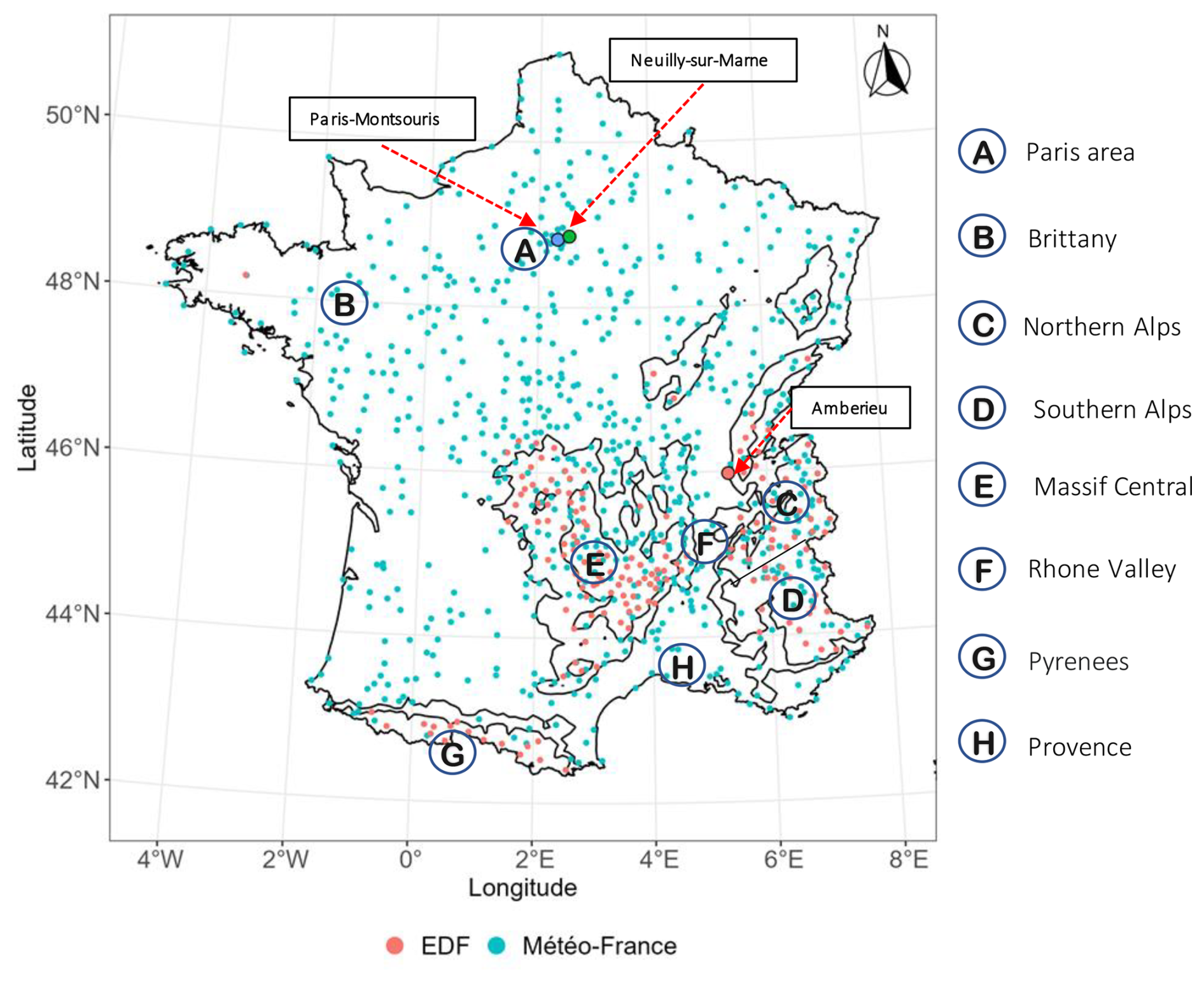
Figure 1 Map of France showing the locations of 934 rain gauges, colored by network affiliation – Météo-France and Électricité de France (EDF). Some stations and locations cited in the article are also depicted. Black solid lines correspond to French borders and the contours around mountainous regions (400 and 800 m elevation).

To explain the observed trends in wet-day precipitation, we incorporate Sea Surface Temperature (SST) anomaly as a covariate within our nonstationary models. Warm SST increases the turbulent near-surface heat fluxes that moisten and destabilize the atmosphere, thereby increasing evaporation and the intensity of convection and precipitation amounts (Funatsu et al., 2009). SST has been widely used as a covariate to explain changes in precipitation (e.g. Senatore et al., 2020) and in the south of France by Tramblay et al. (2013). While other covariates have been used in the literature (e.g. climatic covariates in  Jayaweera et al., 2024), we consider their specific selection to be largely irrelevant for the comparative analysis presented in this study, as all models use the same SST series. In any case, SST provides a stable representation of the thermodynamic changes associated with global warming, allowing for a focused comparison of the internal flexibility of the candidate distributions without the confounding effects of model-selection uncertainty across multiple predictors. A more detailed analysis of covariate selection, including potential regional variations and alternative climate drivers, will form the subject of a future communication.

The SST data we employ in the study was obtained from the NOAA-NCDC Extended Reconstructed Sea Surface Temperature Dataset Version 5 (Huang et al., 2017). We spatially averaged the SST anomalies over the Mediterranean and the proximate Atlantic, specifically spanning longitude 28° W to 19° E and latitude 36 to 58° N (see Fig. 2) . Given our focus on long-term trends, the annual SST values were smoothed using nonparametric locally weighted scatter plot smoothing (LOWESS), implemented via the lowess function in the . Figure 2 illustrates both the raw and smoothed annual SST and the window over which we take the spatial average.

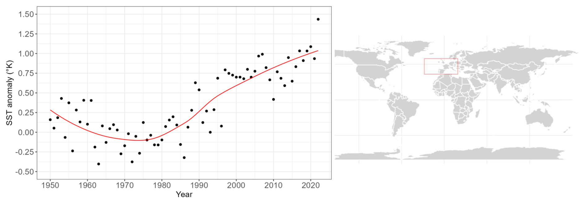
Figure 2 Smoothed sea surface temperature (SST) used as a covariate in the trend analysis. The red box shows the area over which the spatial average was taken.

3 Methodology

This section presents the statistical models that we use, the inference procedure, the comparison framework, as well as the method for uncertainty evaluations.

3.1 Nonstationary models

Let us define Y_t as the random variable of daily precipitation recorded in autumn of a given year t. Y_t can take either zero or positive values depending whether the day is dry or wet, respectively. As a result, modeling daily precipitation, Y_t, requires a mixed model for the discrete (dry-days) and continuous (wet-day intensity) components. Accordingly, the probability that Y_t=0 is $p_{{\mathrm{d}}_t}$, while the probability that Y_t doesn't exceed a given nonzero precipitation amount at a given location can be written as

$$\begin{array}{}\text{(1)}& \mathbb{P}(Y_t\le y)=p_{{\mathrm{d}}_t}+(\mathrm{1}-p_{{\mathrm{d}}_t})\times \mathbb{P}(Y_t\le y|Y_t>\mathrm{0}),\end{array}$$

where $p_{{\mathrm{d}}_t}=\mathbb{P}(Y_t=\mathrm{0})$ is the dry-day probability, and $\mathbb{P}(Y_t\le y|Y_t>\mathrm{0})$ is the wet-day precipitation distribution.

In this study, we employ the same model for the discrete part, which is obtained by fitting a logistic model to the empirical yearly proportion of dry-days in the data, using the year (t) as the covariate. A preliminary analysis (see Fig. A3) revealed time as a better covariate in comparison with SST. The model for the dry-day probability is thus given by:

$$\begin{array}{}\text{(2)}& \log \left({\displaystyle \frac{p_{{\mathrm{d}}_t}}{\mathrm{1}-p_{{\mathrm{d}}_t}}}\right)=p_{{\mathrm{d}}_{\mathrm{0}}}+p_{{\mathrm{d}}_{\mathrm{1}}}t.\end{array}$$

In the case of the continuous part, the usual approach is to make a distributional assumption, where we assume that the marginal distribution of wet-day precipitation, $\mathbb{P}(Y_t\le y|Y_t>\mathrm{0})$ can be represented by a parametric distribution G_t. The subscript (t) indicates that the parameters of the distribution change with time, based on a relationship with some temporal covariate, in our case SST. We will present the form of the relationship later.

Given a specific form for G, the cumulative distribution function (CDF) of Y_t can be written as

$$\begin{array}{}\text{(3)}& F_t\left(y\right)=\mathbb{P}(Y_t\le y)=\left\{\begin{array}{ll}{p}_{{\mathrm{d}}_t}& \text{ if }y=\mathrm{0}\\ p_{{\mathrm{d}}_t}+(\mathrm{1}-p_{{\mathrm{d}}_t})\times G_t\left(y\right),& \text{ if }y>\mathrm{0}\end{array}\right..\end{array}$$

3.1.1 Statistics of interest

From Eq. (3), several statistics of interest can be derived, allowing us to analyze their evolution according to the covariates. We enumerate these key statistics below, as their temporal changes will be a focus of our subsequent analysis.

1. Mean of wet-day distribution. (x_t). Knowing that G_t is the CDF for the wet-day precipitation, its mean, denoted as x_t, can be computed from the expectation of G_t $x_t=\mathbb{E}\left[Y_t\right|Y_t>\mathrm{0}].$

2. Mean of all-day distribution (m_t): The mean of all-day distribution (m_t) can be obtained by accounting for the dry-day probability:

   $$m_t=\mathbb{E}\left[Y_t\right]=(\mathrm{1}-p_{{\mathrm{d}}_t})\times x_t,$$

   where x_t is the mean of the wet-day precipitation as defined above.

3. Quantiles of the wet-day distribution (y_p,t). For a given probability p, the precipitation amount not exceeded in the wet-day precipitation distribution (G_t) is obtained from

   $$\begin{array}{}\text{(4)}& y_{p,t}=G_t^{-\mathrm{1}}\left(p\right).\end{array}$$

4. Return levels. (y_T,t) If the interest is in a given return level, that is an amount that is exceeded, on average, once every T−years, then we have

   $$\begin{array}{}\text{(5)}& y_{T,t}=G_t^{-\mathrm{1}}\left[\mathrm{1}-{\displaystyle \frac{\mathrm{1}}{T\times (\mathrm{1}-p_{{\mathrm{d}}_t})\mathit{\delta }}}\right],\end{array}$$

   where δ is the number of days in the specified season (e.g. δ=92 in autumn).

Finally, we express the percent relative trend for these statistics as:

$$\begin{array}{}\text{(6)}& {\displaystyle \frac{v_{\mathrm{2022}}-v_{\mathrm{1950}}}{\stackrel{\mathrm{‾}}{v}}}\times \mathrm{100},\end{array}$$

where v represents the statistic of interest for example, the mean or a given return level, and $\stackrel{\mathrm{‾}}{v}$ is the average value of that statistic over the entire period 1950 to 2022.

3.1.2 Candidates for the marginal distribution of wet-day precipitation G

The CDFs of the three distribution that we consider in this study are itemized below:

1. Gamma. The CDF of gamma with a location parameter μ>0 and a scale parameter σ>0 is giving by

   $$\begin{array}{}\text{(7)}& G\left(y\right)={\displaystyle \frac{\mathit{\gamma }\left(\frac{\mathrm{1}}{{\mathit{\sigma }}^{\mathrm{2}}},\frac{y}{\mathit{\mu }{\mathit{\sigma }}^{\mathrm{2}}}\right)}{\mathrm{\Gamma }\left({\mathit{\sigma }}^{-\mathrm{2}}\right)}},\end{array}$$

   where Γ(.) and γ(.) are the ordinary gamma and incomplete gamma functions respectively. With this parameterization, the mean is given by μ, while the σ represents the coefficient of variation, i.e the ratio of the standard deviation to the mean of the distribution. Hence, σ controls the spread of the distribution. Under this parameterization, the distribution reduces to exponential when σ=1.

2. Generalized Gamma. Similar to gamma, the CDF of generalized gamma, as implemented in gamlss (Stasinopoulos and Rigby, 2008) is given as:

   $$\begin{array}{}\text{(8)}& G\left(y\right)=\left\{\begin{array}{ll}\frac{\mathit{\gamma }\left(\mathit{\beta },\mathit{\beta }(y/\mathit{\mu }{)}^{\mathit{\nu }}\right)}{\mathrm{\Gamma }\left(\mathit{\beta }\right)}& \text{ if }\mathit{\nu }>\mathrm{0}\\ & \\ \frac{\mathrm{\Gamma }\left(\mathit{\beta },\mathit{\beta }{\left(y/\mathit{\mu }\right)}^{\mathit{\nu }}\right)}{\mathrm{\Gamma }\left(\mathit{\beta }\right)}& \text{ if }\mathit{\nu }<\mathrm{0}\end{array}\right.,\end{array}$$

   with $\mathit{\beta }=\mathrm{1}/\left({\mathit{\sigma }}^{\mathrm{2}}{\mathit{\nu }}^{\mathrm{2}}\right)$. The distribution has three parameters, μ>0, σ>0 and $\mathit{\nu }\ne \mathrm{0},\text{ and }-\mathrm{\infty }<\mathit{\nu }<\mathrm{\infty }$. μ is the location parameter (related to the mean), σ controls the spread, while ν controls the heaviness of the right tail, thereby affecting the magnitude and frequency of extreme events. The distribution is heavy-tailed when ν<1, reduces to gamma when ν=1, and ν>1 indicates a lighter than gamma-tailed model.

3. EGPD.

   $$\begin{array}{}\text{(9)}& G\left(y\right)=\left\{\begin{array}{ll}{\left[\mathrm{1}-(\mathrm{1}+\mathit{\xi }\frac{y}{\mathit{\sigma }}{)}_{+}^{-\mathrm{1}/\mathit{\xi }}\right]}^{\mathit{\kappa }}& \text{ if }\mathit{\xi }\ne \mathrm{0}\\ & \\ {\left[\mathrm{1}-\exp (-\frac{y}{\mathit{\sigma }})\right]}^{\mathit{\kappa }}& \text{ if }\mathit{\xi }=\mathrm{0}.\end{array}\right.,\end{array}$$

   where $a_{+}=max(a,\mathrm{0})$, the flexibility parameter κ>0 controls the lower tail, σ>0 is the scale parameter controlling the spread, and ξ is the shape parameter that controls the upper tail of the distribution. A positive ξ indicates a heavy-tailed distribution, a negative ξ indicates a bounded distribution, while ξ=0 indicates a light-tailed distribution.

3.1.3 Candidate nonstationary models

To account for the possibility of nonstationarity, we identify three cases of nonstationarity in the daily precipitation distribution. They are mainly classified into the following:

1. Stationary case (No trend). Both the dry and wet-day components remain constant over time, with no trend (Row 1 of Table 1).

2. Trend in dry-day frequency only. In this case, only the dry-day frequency exhibits a trend, while the distribution of wet-day precipitation remains stationary (Row 2 of Table 1).

3. Trend in wet-day distribution only. Here, the wet-day precipitation distribution shows a trend, but the dry-day frequency remains stationary (Row 3 of Table 1).

4. Trend in both dry-day frequency and wet-day distribution. Both the dry-day frequency and the wet-day precipitation distribution exhibit concurrent trends (Row 4 of Table 1).

Table 1 Candidate models: The first column indicates the type of nonstationarity. The rest of the columns show the implementation based on the choice of the marginal distribution for the wet-day distribution. In each case, the parameter(s) in the subscript are those that are modeled with a trend component, while the number of parameters to be estimated is enclosed in brackets. ℳ₀ indicates a stationary model.

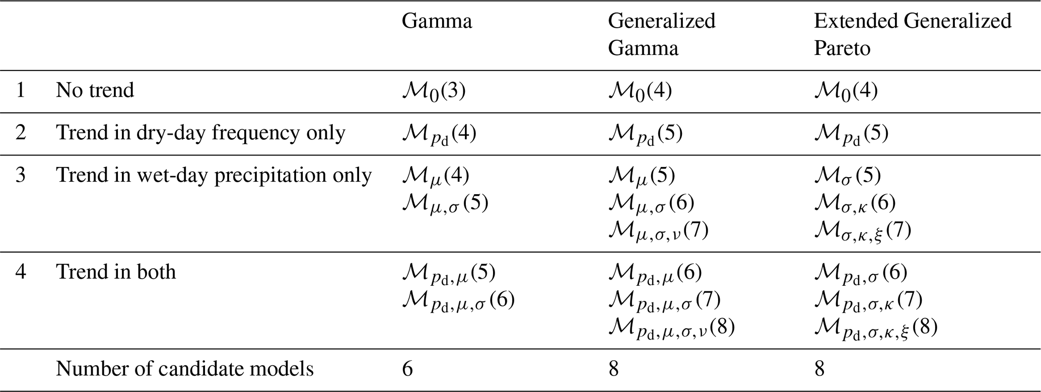
Given the three candidate models for the wet-day distribution (GA, GG, and EGPD) presented in the preceding section, Table 1 outlines the various forms of nonstationarity possible for each. This results in 6 variants for GA (ranging from 3 to 6 parameters), and 8 variants for both GG and EGPD (with parameters ranging from 4 to 8). It is worth noting that the standard practice in extreme value theory, particularly when employing GEV or GPD, often involves keeping the shape parameter ξ stationary (Tramblay et al., 2011; Blanchet et al., 2021b; Evin et al., 2025). This approach is typically justified by concerns regarding parameter instability and estimation difficulties due to data limitations. However, in our study, data quantity is not a limitation as we utilize all nonzero daily observations in our inference procedure, allowing us to explore nonstationarity in the shape parameter.

Irrespective of the model, a linear relationship is assumed between the model parameter and SST according to

$$\begin{array}{}\text{(10)}& \mathit{\eta }\left({\mathit{\alpha }}_t\right)={\mathit{\alpha }}_{\mathrm{0}}+{\mathit{\alpha }}_{\mathrm{1}}{\mathrm{SST}}_t,\end{array}$$

where α represents a given nonstationary parameter of GA, GG, or EGPD. η is a transformation applied to α, depending on its valid range; it is logarithmic for parameters defined on the positive real line and identity otherwise.

3.2 Inference

We use the method of maximum likelihood estimation to infer the parameters of our models. The likelihood of the mixed distribution for a single year t, assuming independent observations, can be written as:

$$\begin{array}{}\text{(11)}& L_t\left({\mathit{\psi }}_t\right)=\left(\prod _{j=\mathrm{1}}^{s_t}{p}_{{\mathrm{d}}_t}\right)\cdot \left(\prod _{j=\mathrm{1}}^{w_t}\left(\mathrm{1}-p_{{\mathrm{d}}_t}\right)\cdot g_t\left(y_{j,t}\right)\right),\end{array}$$

where for year t, y_j,t is the jth daily precipitation, g_t is the PDF of wet-day precipitation, ${\mathit{\psi }}_t=\mathit{\{}{p}_{{\mathrm{d}}_t},{\mathit{\theta }}_t\mathit{\}}$ is the vector of all model parameters, with θ_t the vector of parameters of g_t, D_t is the total number of days , s_t is the number of dry days, and w_t the number of wet days in year t such that $D_t=s_t+w_t$.

The corresponding log-likelihood for a single year t is then:

$$\begin{array}{}\text{(12)}& \begin{array}{rl}{\mathrm{\ell }}_t\left({\mathit{\psi }}_t\right)& =s_t\log \left(p_{{\mathrm{d}}_t}\right)+w_t\log (\mathrm{1}-p_{{\mathrm{d}}_t})\\ & +\sum _{j:y_{j,t}>\mathrm{0}}\log \left[g_t\right(y_{j,t}\left)\right].\end{array}\end{array}$$

For the total observation period across all N years, the overall log-likelihood function to be maximized is:

$$\begin{array}{}\text{(13)}& \begin{array}{rl}\mathrm{\ell }\left(\mathit{\psi }\right)& =\sum _{t=\mathrm{1}}^N{\mathrm{\ell }}_t\left({\mathit{\psi }}_t\right)=\sum _{t=\mathrm{1}}^N\mathit{\left\{}{s}_t\log \right(p_{{\mathrm{d}}_t})+w_t\log (\mathrm{1}-p_{{\mathrm{d}}_t})\\ & +\sum _{j:y_{j,t}>\mathrm{0}}\log \left[g_t\right(y_{j,t}\left)\right]\mathit{\}}\end{array}\end{array}$$

Here, ψ contains all the parameters that define nonstationary relationships (e.g. $p_{{\mathrm{d}}_{\mathrm{0}}}$, $p_{{\mathrm{d}}_{\mathrm{1}}}$ for dry-day and α₀, α₁ for wet-day parameters as introduced in Eqs. 2 and 10).

To estimate ψ by maximum likelihood, one can directly maximize the overall log-likelihood in Eq. (13). Alternatively, the parameters of the dry-day and wet-day precipitation components can be estimated separately by maximum likelihood. We have tried both and they yield similar estimates. For the remainder of this study, we adopt the second approach. The overall log-likelihood (Eq. 13) is then calculated using the estimated parameters for subsequent model comparison.

3.3 Model selection

3.3.1 AIC

The model selection is through the use of the Akaike Information Criteria (AIC) (Akaike, 1974) that rewards goodness-of-fit as measured by the likelihood as well as parsimony, in terms of the number of free parameters. We adopt AIC because our primary objective is predictive performance rather than identifying a single true model of fixed dimension (see Chakrabarti and Ghosh, 2011), an assumption that is unlikely to hold for stochastic rainfall processes. AIC has also been widely applied for model selection under nonstationarity (e.g. Kim et al., 2017; Jayaweera et al., 2024). The criterion is computed from $\mathrm{AIC}=\mathrm{2}K-\mathrm{2}\mathrm{\ell },$ where K is the number of parameters of a given model (see Table 1) and ℓ is the log-likelihood from Eq. (13). The best model among candidate models is the one with the minimum value of AIC.

3.3.2 Model Diagnostics

In addition to the AIC, we conduct a detailed diagnostic analysis to assess the performance of our candidate nonstationary models. Specifically, we evaluate how well each model captures relative trends v(%) (Eq. 6) in key precipitation statistics, compared to those estimated using established benchmark approaches. We consider the four statistics introduced in Sect. 3.1.1. They are: (i) the mean of wet-day precipitation (x_t), (ii) the mean of all-day precipitation (m_t), (iii) wet-day quantiles (y_p,t), and (iv) 10-year return level.

The benchmark methods we use as references are given below:

1. For the mean of wet-day precipitation (x_t) and the mean of all-day precipitation (m_t), we use a nonparametric approach based on the Theil-Sen slope estimator (Theil, 1950; Sen, 1968). This approach to trend estimation calculates the slopes between all possible pairs of data points in the time series and defines the overall trend as the median of all these slopes. Unlike Ordinary Least Squares (OLS), it is insensitive to outliers.

2. In the case of wet-day quantiles (y_p,t), we employ a nonparametric quantile regression (QR) with total variation roughness penalties (Koenker and Mizera, 2004). While standard regression models the trend in the mean, QR estimates the trend at specific quantiles (e.g., the 0.5, 0.95, or 0.99). We use the quantreg R package to fit these trends, using the same SST covariate used in our parametric models. To assess the performance of our candidate model in both low, medium, and high quantiles, we extract the trends at $p\in \mathit{\{}\mathrm{0.2},\mathrm{0.3},\mathrm{0.4},\mathrm{0.5},\mathrm{0.6},\mathrm{0.7},\mathrm{0.8},\mathrm{0.9},\mathrm{0.95},\text{and }\mathrm{0.98}\mathit{\}}$ and compare them to those obtained using QR.

3. For the 10-year return level, we consider the estimated trends from a nonstationary GEV model fitted to the seasonal block maxima. At each station, we fit three versions of the NS-GEV and selected the one with the lowest AIC. The versions are: GEV-ℳ_μ, GEV-ℳ_σ and GEV-ℳ_μ,σ, where μ and σ are the GEV location and scale parameters. In each case, we use SST as the covariate, as is the case in our candidate models.

This process yields, for each model and each statistic, a set of 934 trend estimates, one per station, which are then compared directly to the 934 benchmark estimates for the same stations. A well-performing model is expected to closely match the benchmark trends across stations, both in direction and magnitude. To quantify the agreement, we utilize the Concordance Correlation Coefficient (CCC)

$$\begin{array}{}\text{(14)}& \mathrm{CCC}={\displaystyle \frac{\mathrm{2}\mathit{\rho }{\mathit{\sigma }}_x{\mathit{\sigma }}_y}{{\mathit{\sigma }}_x^{\mathrm{2}}+{\mathit{\sigma }}_y^{\mathrm{2}}+{\left({\mathit{\mu }}_x-{\mathit{\mu }}_y\right)}^{\mathrm{2}}}}\end{array}$$

where ρ is the Pearson correlation.

This metric provides a comprehensive measure of the agreement in both the direction and magnitude of the trends. Being a correlation measure, it takes values from −1 to 1, with 1 indicating perfect correlation. While classical correlation measures like Pearson's and Spearman's coefficients measure the linear or monotonic relationship, they are insensitive to bias or scale differences in the two variables. This is why we employ CCC, which measures the agreement, penalizing both scale and bias differences (the ${\left({\mathit{\mu }}_x-{\mathit{\mu }}_y\right)}^{\mathrm{2}}$ term).

3.4 Trend significance and uncertainties

We assess the uncertainty and significance of a given trend through nonparametric bootstrap as done in Haruna et al. (2025); Evin et al. (2025). To implement this, the trend for a given statistic of interest is re-estimated from bootstrap samples, which are generated by sampling with replacement from the original data. This resampling procedure is repeated 400 times, giving 400 sets of parameters. A trend is considered statistically significant if zero is not contained within the 2.5 % and 97.5 % empirical centiles of its bootstrap estimates. We comment here that the resampling is applied to the residuals of the original sample, rather than directly to the raw data. This approach ensures that the bootstrap samples are identically distributed. The residuals are obtained by applying the CDF of the given nonstationary model to the original sample. The bootstrap samples of residuals are then back-transformed using the quantile function of the nonstationary model to generate new precipitation series for trend estimation. For a more detailed exposition of this bootstrap procedure, readers are referred to Sect. 3.4 of Haruna et al. (2025).

4 Results

4.1 Goodness-of-fit and model selection

This section presents a graphical diagnostic of the goodness-of-fit of some of the fitted models at some randomly selected stations. Next, we show the results of the model selection based on AIC.

4.1.1 Graphical diagnostics: Quantile-Quantile plots

We start with a diagnostic analysis to rigorously assess the goodness-of-fit of the models, utilizing graphical diagnostics, in this case, residual quantile–quantile (Q–Q) plots. Compared to classical Q–Q plots, residual Q–Q plots are relevant in the case of data that are not identically distributed (Coles et al., 2001). To produce the plots, we first transform the data for each year using the CDF derived from the fitted nonstationary model. When the model is correctly specified, this transformation yields uniformly distributed data within the interval (0, 1). Next, we transform this uniformly distributed data using the inverse CDF of the exponential distribution. Consequently, the data become approximately identically distributed according to the exponential distribution. Using the exponential distribution facilitates the creation of effective Q–Q plots with a clearer visualization of the upper tail. Figure 3 showcases the exponentiated quantile residual plots at some randomly selected stations. In each case, the points are colored according to the given distribution. Note that in the figure, the most flexible variant of each distribution is considered; ${\mathcal{M}}_{p_{\mathrm{d}},\mathit{\mu },\mathit{\sigma }}$ for GA, ${\mathcal{M}}_{p_{\mathrm{d}},\mathit{\mu },\mathit{\sigma },\mathit{\nu }}$ for GG and ${\mathcal{M}}_{p_{\mathrm{d}},\mathit{\kappa },\mathit{\sigma },\mathit{\xi }}$ in the case of EGPD. For a good model, the points should lie on the diagonal, here shown by the dashed line. In general, for all the cases shown here, all the points lie reasonably close to the diagonal, showcasing a good model fit. A few exceptions can be observed, with some deviations around the tail. Note that the Q–Q plots shown here are just for illustration of the model fit, rather than a comparison, due to the difference in the number of parameters of the models. A more flexible model is in general expected to perform better in comparison to a less flexible model. The next section uses AIC, which accounts for model complexity, to compare and rank the models.

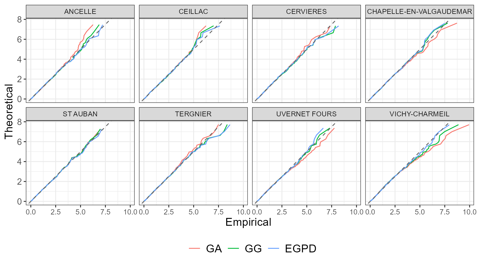
Figure 3 Illustration of model fits using exponentiated quantile residuals plots at some selected stations. The three models are gamma (GA-${\mathcal{M}}_{p_{\mathrm{d}},\mathit{\mu },\mathit{\sigma }}$), generalized gamma (GG-${\mathcal{M}}_{p_{\mathrm{d}},\mathit{\mu },\mathit{\sigma },\mathit{\nu }}$) and, extended generalized Pareto (EGPD-${\mathcal{M}}_{p_{\mathrm{d}},\mathit{\kappa },\mathit{\sigma },\mathit{\xi }}$).

4.1.2 AIC: Intramodel comparison

This section presents the model selection results based on AIC, applied separately to the variants of each candidate wet-day distribution (GA, GG and EGPD). Figure 4 illustrates these results for all three distributions. In each subplot of Fig. 4, stationary models (indicating no trend) are represented by black-filled circles. Models incorporating a trend solely in the dry-day frequency are shown with yellow-filled circles. Models with trends exclusively within the wet-day distribution are depicted by square shapes, with varying shades of maroon. The darker the color, the higher the complexity of the model in terms of the number of parameters. Lastly, models featuring trends in both dry-day frequency and wet-day distribution are indicated by triangular shapes, with various shades of green. Across all three maps, there is a strong agreement in the spatial coherence of the selected model forms for nonstationarity, particularly evident between the two three-parameter distributions (GG and EGPD). Observing the regional patterns, especially in the northern and western parts of France (excluding areas along the Pyrenees), models with either a trend in dry-day frequency (yellow) or trends in both components (green triangular shapes) are consistently selected, regardless of the chosen wet-day distribution. A similar pattern emerges along the northern Alps and some locations along the southern part of the Massif Central, where models showing trends only in the wet-day distribution (maroon-colored square shapes) are favored. Finally, there is also notable agreement in locations where stationary models (black-colored circles) are selected, specifically at some stations along the Pyrenees and near the Mediterranean. Figure 5 further summarizes the number of stations corresponding to each form of nonstationarity across the three distributions, confirming the high degree of similarity, especially between the GG and EGPD.

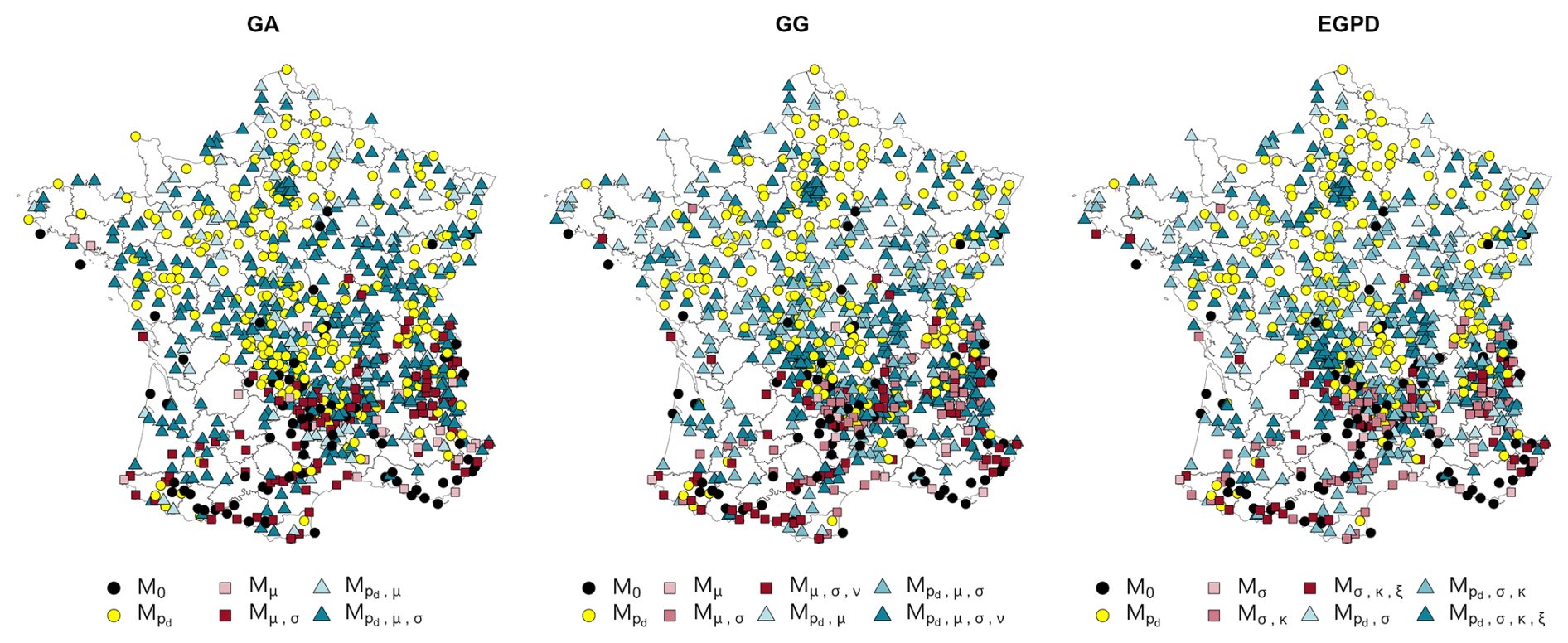
Figure 4 Maps showing the model selection results based on AIC applied to the variants of each distribution separately. Each station is colored according to the best model. Stationary models (indicating no trend) are shown by black-filled circles. Models with trend in only the dry-day frequency are shown with yellow-filled circles. Models with trends in only the wet-day distribution are depicted by square shapes, with varying shades of maroon. Lastly, models featuring trends in both dry-day frequency and wet-day distribution are indicated by triangular shapes, with various shades of green. The darker the color, the higher the complexity of the model in terms of the number of parameters.

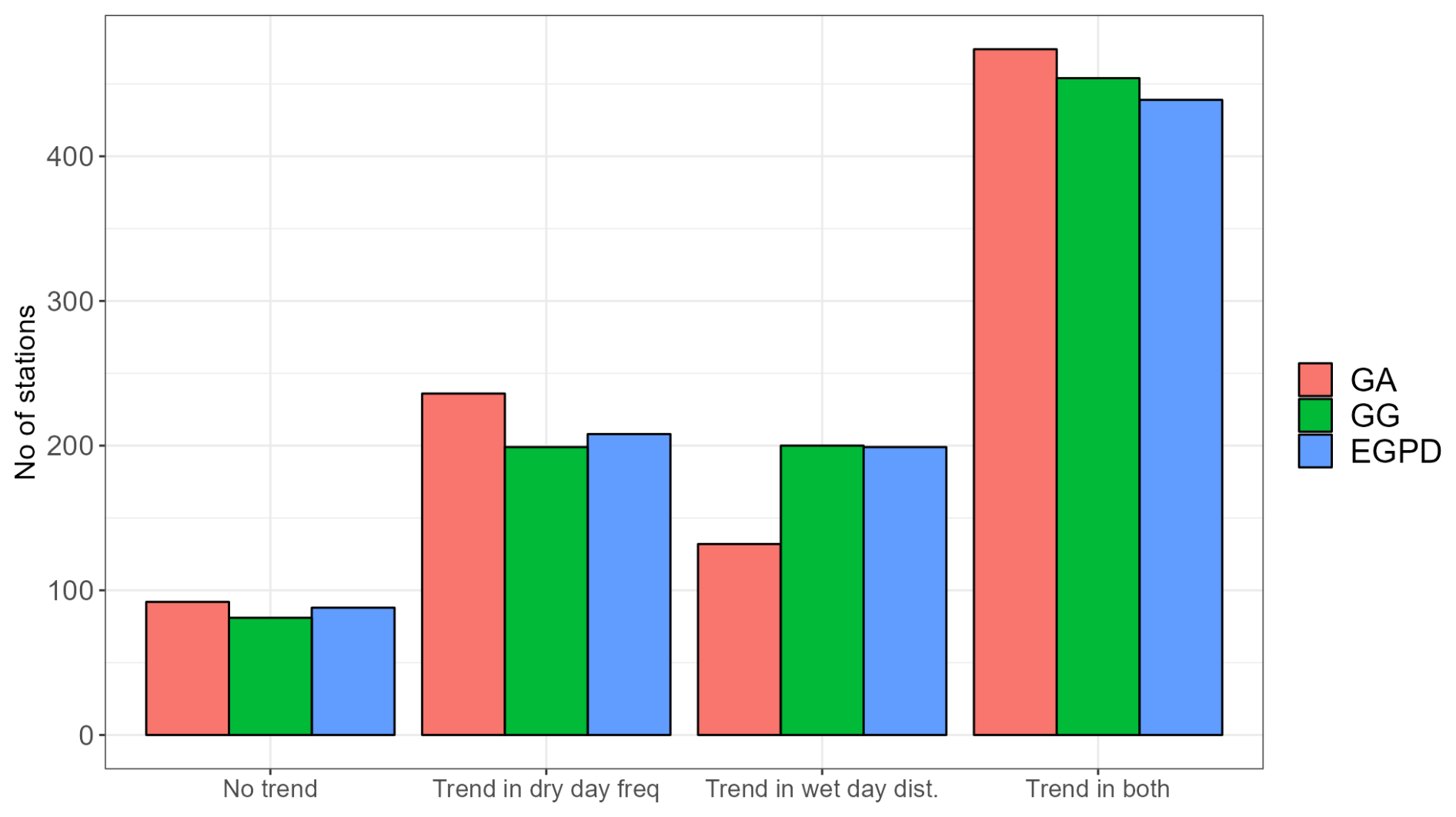
Figure 5 Number of stations with a given type of nonstationarity (horizontal axis) selected based on AIC.

4.1.3 AIC: Intermodel comparison

We now proceed with the overall model selection based on AIC, irrespective of the initial distributional family. To achieve this, we compared the AIC of the best model (chosen in the preceding “Intramodel Comparison” section) from each of the three candidate distributions – GA, GG, and EGPD. The model with the lowest AIC value among these three is then selected as the overall best-performing model for that specific station. Figure 6 showcases the result of this selection. Each station is colored according to the best-performing distribution. In summary, the GG emerges as the preferred distribution in the majority of locations (68 %), followed by EGPD in 22 % of cases, and finally, GA in 10 %. There is no clear spatial pattern for the stations where the Gamma distribution is selected. For EGPD, however, the model appears to be favored in the region around the northeast of the Massif Central.

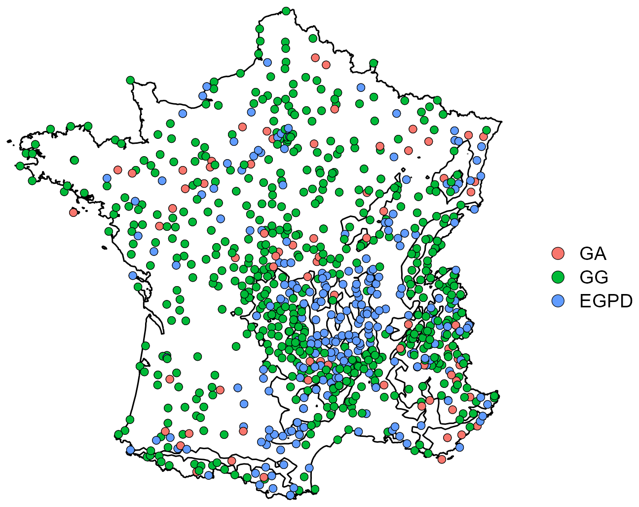
Figure 6 Model selection result based on AIC irrespective of the initial distributional family. Each station is colored according to the best-performing distribution, while shapes are used to illustrate the corresponding type of nonstationarity identified.

4.2 Model performance in capturing trends evolutions

While the AIC provides a solid theoretical justification for model selection by balancing goodness-of-fit and parsimony, we take a further step to evaluate the models based on their performance in reproducing relative trends (v(%)). We compare our models' outputs against benchmark relative trends (v(%)) obtained through nonparametric QR and nonstationary GEV models, as detailed in Sect. 3.3.2. This evaluation involves checking the trends in: (i) the mean of wet-day and all-day precipitation; (ii) low, medium, and high quantiles of the wet-day distribution; and (iii) extreme precipitation. The results are presented in the following subsections.

4.2.1 Trend in wet-day quantiles

Given that a reliable model should accurately capture trends across the entire wet-day precipitation distribution, including low, medium, and high quantiles, we compare the performance of our candidate models using QR as a nonparametric benchmark. Figure 7 shows the scatter plots (top row) of the nonzero precipitation (points) at three stations (see locations in Fig. 1), along with time-evolving wet-day quantiles (y_p,t) estimated with QR, for $p\in \mathit{\{}\mathrm{0.2},\mathrm{0.5},\mathrm{0.8},\mathrm{0.9},\mathrm{0.95},\mathrm{0.98}\mathit{\}}$ (colored-lines). The three stations exhibit contrasting behaviors in terms of the trend direction. Neuilly-sur-Marne has all the quantiles decreasing with time (unidirectional behavior), Amberieu has its low quantiles decreasing and the high quantiles increasing with time (bidirectional), while Paris-Montsouris has a negative trend in the lowest quantiles, transitioning to positive trends in the medium quantiles, and then reverting to negative in the highest quantiles (tridirectional). A good model among our candidate models should be able to reproduce all this behavior.

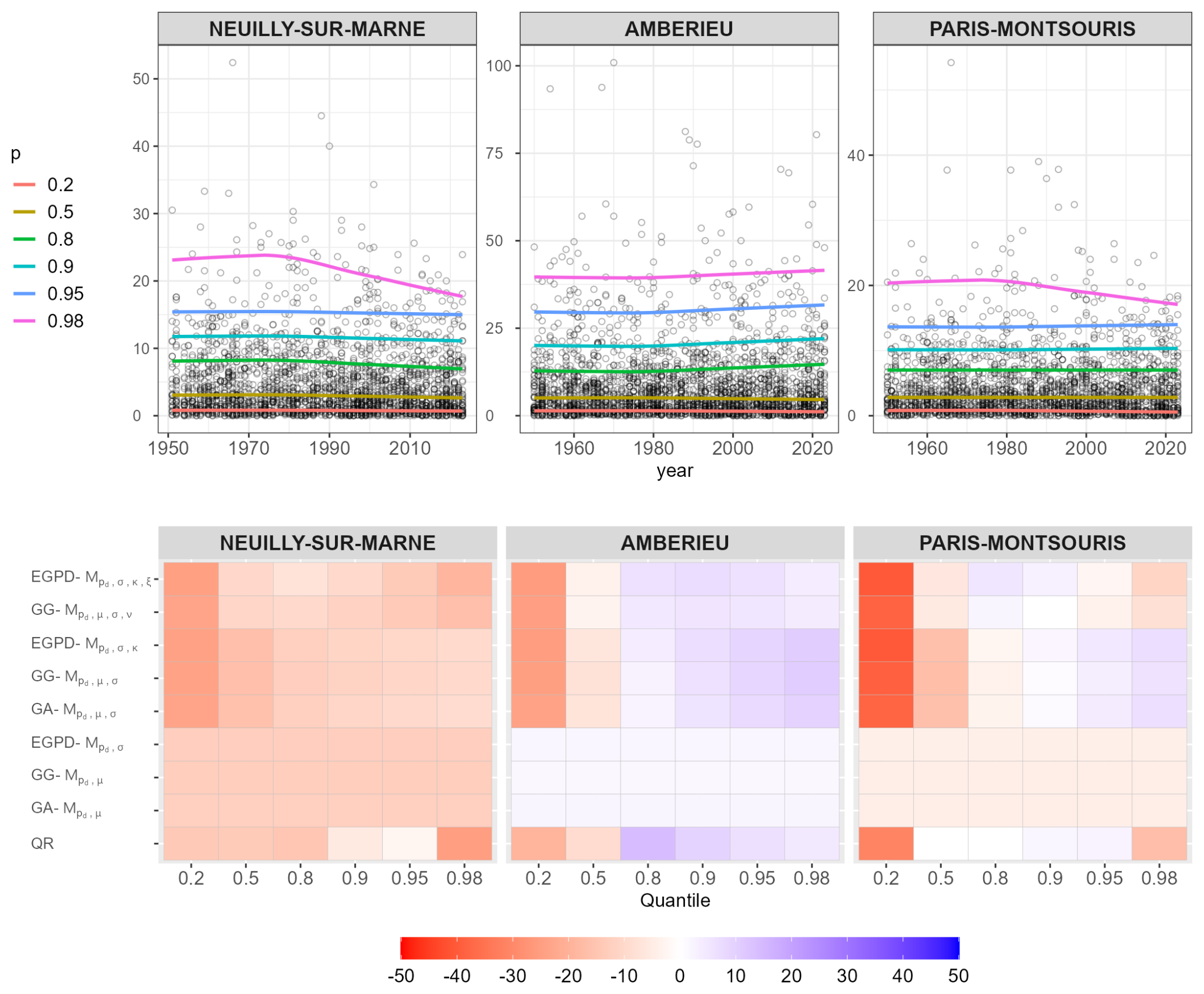
Figure 7 Comparison of quantile trend evolutions for selected stations. The top row shows the time series plot of nonzero precipitation along with time-evolving quantiles predicted with nonparametric QR. The bottom row depicts the tile plots of relative trends (v(%)), estimated with QR and the candidate model, colored according to the trend direction (blue for positive trends, red for negative trends). The horizontal axis represents the quantile.

The second row presents the tile plots of relative trends (v(%)) estimated with QR and the candidate models for the three stations, colored according to the trend direction (blue for positive, red for negative). The quantiles are given on the horizontal axis, while the candidate models are depicted on the vertical axis, arranged from bottom to top, in order of complexity (number of free parameters). The models with the lowest flexibility, having only a single wet-day parameter varying with SST (GA-${\mathcal{M}}_{p_{\mathrm{d}},\mathit{\mu }}$, GG-${\mathcal{M}}_{p_{\mathrm{d}},\mathit{\mu }}$, and EGPD-${\mathcal{M}}_{p_{\mathrm{d}},\mathit{\sigma }}$), resulted in a single trend irrespective of the quantile and station. Notice in the case of Neuilly-sur-Marne with unidirectional behavior, although these models predicted a decreasing trend, the trends are independent of the quantile level. The models with two wet-days parameters evolving with SST (GA-${\mathcal{M}}_{p_{\mathrm{d}},\mathit{\mu },\mathit{\sigma }}$, GG-${\mathcal{M}}_{p_{\mathrm{d}},\mathit{\mu },\mathit{\sigma }}$, and EGPD-${\mathcal{M}}_{p_{\mathrm{d}},\mathit{\sigma },\mathit{\kappa }}$) are able to show a bidirectional behavior, with negative trends for the smallest quantiles, and positive trends for the highest quantiles in the case of Amberieu which show a bidirectional behavior. The tridirectional behavior in the case of Paris-Montsouris is only reproduced with the most flexible models (GG-${\mathcal{M}}_{p_{\mathrm{d}},\mathit{\mu },\mathit{\sigma },\mathit{\nu }}$, and EGPD-${\mathcal{M}}_{p_{\mathrm{d}},\mathit{\sigma },\mathit{\kappa },\mathit{\xi }}$) as revealed by QR.

To generalize the result across all the stations, we use the Concordance Correlation Coefficient (CCC) (detailed in Sect. 3.3.2) to quantitatively assess the agreement between the relative trends (v(%)) from our models and those from QR. For each quantile p, we compute the CCC between the trends estimated with QR and each of the candidate models. The best model among the candidate models should have CCC = 1, signifying a perfect agreement with QR for that quantile level. The results is presented in Fig. 8. In the figure, GA models are depicted in shades of maroon, GG models in shades of green, and EGPD models in shades of blue; in each case, a darker shade denotes a more flexible model (i.e., more parameters changing with SST). Analyzing result, the GG model ${\mathcal{M}}_{p_{\mathrm{d}},\mathit{\mu },\mathit{\sigma },\mathit{\nu }}$ demonstrated the highest agreement with QR for virtually all quantiles. It is closely followed by the EGPD model ${\mathcal{M}}_{p_{\mathrm{d}},\mathit{\kappa },\mathit{\sigma },\mathit{\xi }}$. The least flexible models, with only one parameter changing with SST, irrespective of the distribution, have the lowest correlation. It is worth noting that, irrespective of the criterion, all the models have nearly similar performance within the bulk of the distribution (around p=0.7), but the disparity appears around the tails, especially the upper tail. The most flexible models GG model ${\mathcal{M}}_{p_{\mathrm{d}},\mathit{\mu },\mathit{\sigma },\mathit{\nu }}$ and the EGPD model ${\mathcal{M}}_{p_{\mathrm{d}},\mathit{\kappa },\mathit{\sigma },\mathit{\xi }}$ in particular standout in their exclusive performance in the upper tail, where the other less flexible models have much lower performance. This strongly suggests that the increased flexibility of these models is indeed justified for accurately capturing the complex trend evolutions observed across the entire range of the precipitation dataset.

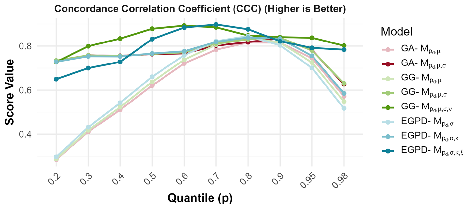
Figure 8 Comparison of model performance in reproducing relative trend in wet-day quantiles. The figure shows the Concordance Correlation Coefficient (CCC) computed between the relative trends estimated with QR and each of the candidate models at all the stations. Gamma (GA) models are in shades of maroon, Generalized Gamma (GG) models in shades of green, and Extended Generalized Pareto Distribution (EGPD) models in shades of blue. Darker shades indicate more flexible models (more parameters evolving with SST).

4.2.2 Trend in mean precipitation

The maps of the relative trends in mean wet-day precipitation (x_t) from our candidate models alongside a nonparametric benchmark based on Theil-Sen slope estimator are shown in Fig. 9. The top row showcases trends predicted by the three GG model variants. The second row corresponds to the three EGPD model variants, while the first two maps in the bottom row represent the two GA model variants. The map on the bottom-right illustrates trends derived using the Theil-Sen slope estimator. In general, all the models exhibit a similar spatial pattern in both the magnitude and direction of trends when compared to those obtained with the Theil-Sen slope method. This strong agreement is quantitatively confirmed by a Concordance Correlation Coefficient (CCC) close to one for all the models. While all models yield very satisfying results, GA-${\mathcal{M}}_{p_{\mathrm{d}},\mathit{\mu }}$ notably demonstrates the best performance. This can be attributed to its direct parametrization, where the evolving parameter μ is precisely the mean of the Gamma distribution itself. For the case of the mean of all-day precipitation (m_t), the performance of the models is nearly indistinguishable. The maps of the trends for this statistic are provided in Fig. A1.

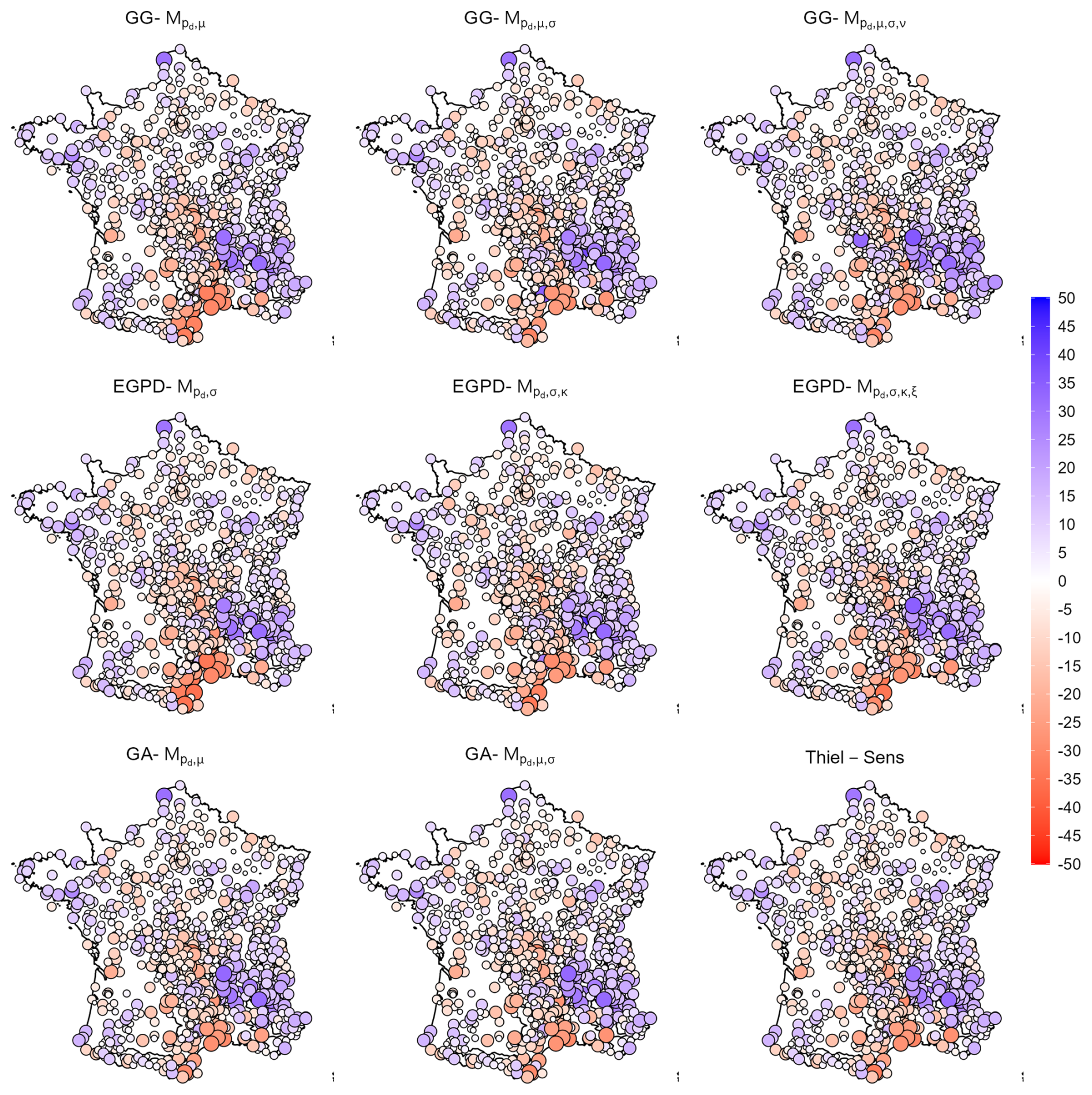
Figure 9 Maps of relative trends (%) in mean wet-day precipitation (x_t) for various nonstationary models and the Theil-Sen benchmark. Top row: GG models. Second row: EGPD models. Bottom row (first two maps): GA models. Bottom-right map: Trends obtained using the nonparametric Theil-Sen slope estimator (benchmark).

4.2.3 Trend in extreme precipitation

In this section, we compare the performance of the models in terms of the relative trends in extreme precipitation, specifically focusing on the 10-year return level (y_10,t). To serve as a benchmark, we use a nonstationary GEV model (NS-GEV) by parameterizing μ and/or σ as linear functions of SST to estimate these trends. Figure 10 illustrates some return level plots at three stations (the same stations shown in Fig. 7), comparing the trends obtained with GEV benchmark and the most flexible version of each of the three distributions (GA-${\mathcal{M}}_{p_{\mathrm{d}},\mathit{\mu },\mathit{\sigma }}$, GG-${\mathcal{M}}_{p_{\mathrm{d}},\mathit{\mu },\mathit{\sigma },\mathit{\nu }}$, and EGPD-${\mathcal{M}}_{p_{\mathrm{d}},\mathit{\sigma },\mathit{\kappa },\mathit{\xi }}$). For all the stations, the least agreement is obtained with GA-${\mathcal{M}}_{p_{\mathrm{d}},\mathit{\mu },\mathit{\sigma }}$. This is more apparent in the case of Paris-Montsouris, where the model predicts an opposing trend evolution compared to the other models, both for the 2-year and 10-year return level.

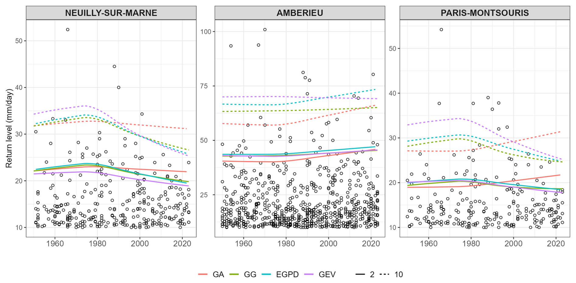
Figure 10 Comparison of 2-year and 10-year return levels evolution for selected stations. Each panel displays return levels from the GEV benchmark (purple line) and the most flexible variant of each candidate distribution: GA-ℳ_μ,σ (orange line), GG-${\mathcal{M}}_{\mathit{\mu },\mathit{\sigma },\mathit{\nu }}$ (lime-green line), and EGPD-${\mathcal{M}}_{\mathit{\sigma },\mathit{\kappa },\mathit{\xi }}$ (cyan line). The horizontal axis indicates the year, vertical axis is the precipitation amount.

Figure 11 shows the maps of the relative trends (%) in a 10-year return level estimated by our candidate models and the GEV over all the stations in the study area. Similar to Fig. 9, the top rows show the trend predicted with the three GG models, the second row corresponds to the three EGPD models, while the first two maps in the bottom row correspond to the two GA models. The map on the bottom right corresponds to the trends obtained using the GEV. A first look at the spatial pattern reveals a column-wise similarity. The first column corresponds to models with only one nonstationary parameter. With these models, the trend is generally positive or close to zero in the north and the southwest. Negative trends are mainly observed near the Provence in the south and the northwest of the Massif Central. The second column, which represents models with nonstationarity in two parameters, exhibits spatial patterns similar to those in the first column but with generally higher magnitudes of trends. A significant increase in the contrast of the spatial pattern of trends is observed in the last column, which corresponds to the most flexible models with three parameters (GG-${\mathcal{M}}_{p_{\mathrm{d}},\mathit{\mu },\mathit{\sigma },\mathit{\nu }}$, and EGPD-${\mathcal{M}}_{p_{\mathrm{d}},\mathit{\sigma },\mathit{\kappa },\mathit{\xi }}$). This column reveals a distinct cluster of stations with negative trends around the Parisian area and the northeast, a pattern not as pronounced in less flexible variants. Furthermore, stronger negative trends are now evident in the southeastern and western sides of the Massif Central. This pattern is in close agreement with the trends modeled using the GEV benchmark.

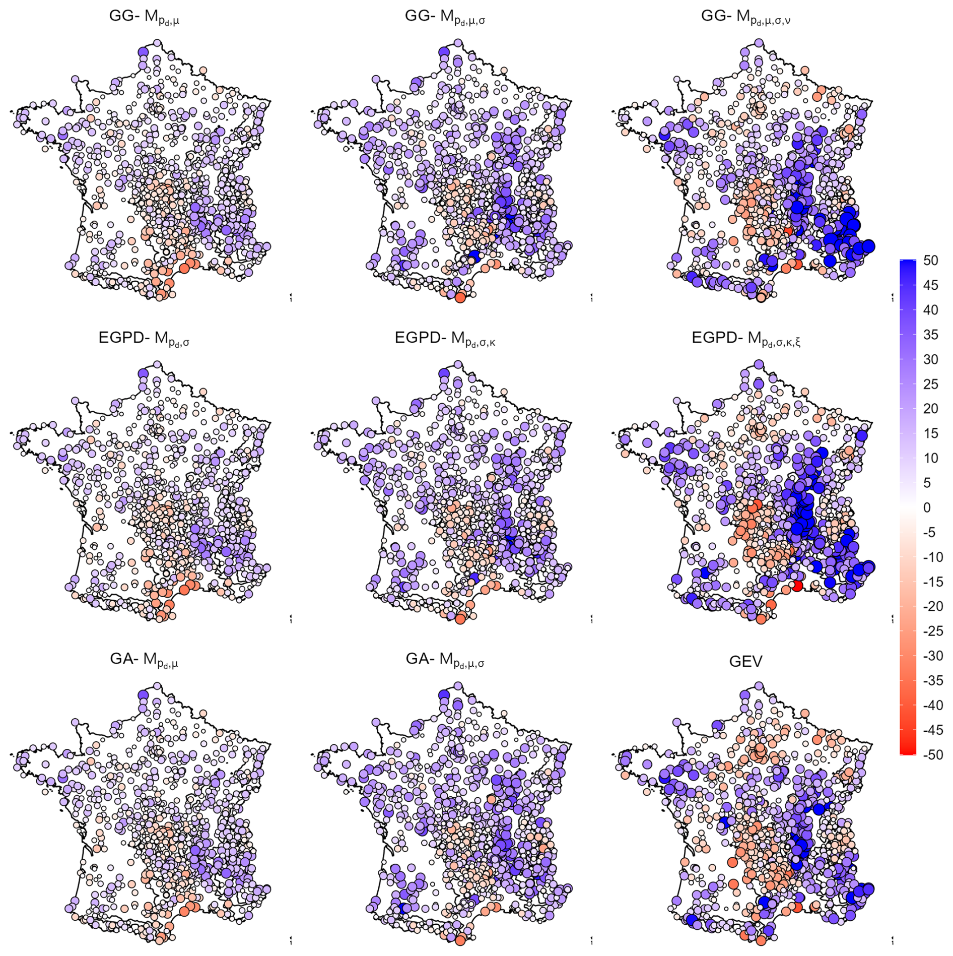
Figure 11 Maps of relative trends (%) in the 10-year return level (y_10,t) for various nonstationary models and the GEV benchmark. Top row: GG models. Second row: EGPD models. Bottom row (first two maps): GA models. Bottom-right map: Trends obtained using the nonstationary GEV model (benchmark).

Finally, to obtain a quantitative measure of the model's performance, we apply the Concordance Correlation Coefficient between the relative trend estimates obtain with the GEV and each of the candidate models. The results show that the GG-${\mathcal{M}}_{p_{\mathrm{d}},\mathit{\mu },\mathit{\sigma },\mathit{\nu }}$, and EGPD-${\mathcal{M}}_{p_{\mathrm{d}},\mathit{\sigma },\mathit{\kappa },\mathit{\xi }}$ have the closest agreement with GEV (CCC = 0.8) compared to the other models with CC ranging from 0.4 to 0.55.

4.3 Observed trends and uncertainties with the best model

Our two complementary model comparison approaches, AIC-based selection and models' ability to capture trends, consistently point to similar conclusions regarding the most suitable distribution and its most effective nonstationary variant. The first approach, based on AIC, revealed GG as the favored distribution at 68 % of the stations compared to 22 % for the EGPD and 20% for the GA. The second approach, which rigorously assesses the models' ability and flexibility in capturing trends across the entire precipitation spectrum, also largely favored GG, and in particular the most flexible variant GG-${\mathcal{M}}_{p_{\mathrm{d}},\mathit{\mu },\mathit{\sigma },\mathit{\nu }}$. It is important to note that EGPD performed very similarly to GG in terms of trend reproduction. For instance, even when AIC more frequently selected GG variants, the spatial patterns of the best-performing variants for both GG and EGPD were strikingly similar (Figs. 4 and 5). More interestingly, both the GG-${\mathcal{M}}_{p_{\mathrm{d}},\mathit{\mu },\mathit{\sigma },\mathit{\nu }}$ and EGPD-${\mathcal{M}}_{p_{\mathrm{d}},\mathit{\sigma },\mathit{\kappa },\mathit{\xi }}$ models exhibited very similar, strong performances across the CCC, especially across wet-days quantiles and extreme preciptation. In contrast, the Gamma distribution, even its most flexible variant (GA-${\mathcal{M}}_{p_{\mathrm{d}},\mathit{\mu },\mathit{\sigma }}$), consistently proved unable to adequately reproduce the observed complex trends.

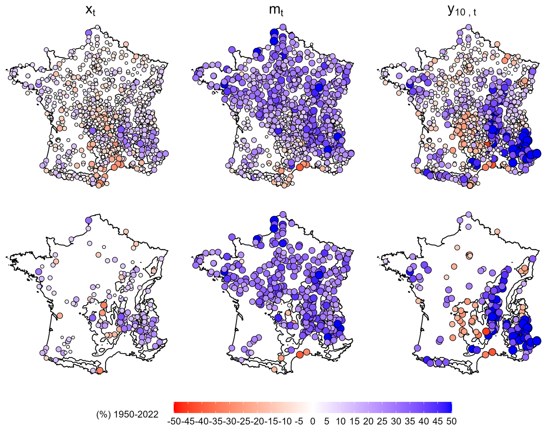
Figure 12 Maps of relative trends and their significance for the selected best model (GG-${\mathcal{M}}_{p_{\mathrm{d}},\mathit{\mu },\mathit{\sigma },\mathit{\nu }}$). The top row shows trends in the mean of wet-day precipitation (x_t), the mean of all-day precipitation (m_t), and the 10-year return level (y_10,t). Negative trends are shown in red, while positive trends are in blue. The bottom row shows the same maps, but only where the trends are statistically significant based on the nonparametric bootstrap procedure (Sect. 3.4).

Based on the results, therefore, we consider GG as the best distribution and, in particular, the variant GG-${\mathcal{M}}_{p_{\mathrm{d}},\mathit{\mu },\mathit{\sigma },\mathit{\nu }}$ to be a viable choice for modeling nonstationary daily precipitation in this region. The top row of Fig. 12 shows the relative trends obtained in the case of the mean of wet-day precipitation (x_t), the mean of all-day precipitation (m_t), and a 10-year return level y_10,t. Negative trends are shown in red, while positive trends are shown in blue. The bottom row shows the same trends, but masking the nonsignificant trends based on the bootstrap procedure described in Sect. 3.4. The figure reveals a significant increase in the mean of wet-day precipitation, notably in the southeastern part. The mean of all-day precipitation, on the other hand, shows a significant increase everywhere, except the southwestern region. In terms of extreme precipitation, significant positive trends in the 10-year return level appear along the Rhone valley, the southeast, and some locations around Brittany. Significant negative trends are obtained at some locations in the northern Alps and the western side of the Massif Central. While this illustrates the modeled trends, a more detailed spatial and seasonal analysis of these trends and a deeper investigation of covariate selection will be the subject of subsequent communications.

5 Discussion

This study presents a comprehensive comparison framework for selecting the best nonstationary model of daily precipitation using a mixed discrete-continuous distribution, driven by SST and time as a key covariates. By evaluating various distributional families (GA, GG, EGPD) and their nonstationary variants, our approach moves beyond traditional stationary or simpler nonstationary methods to provide a more refined understanding of precipitation trends. We have chosen France as a case study due to its wide diversity of climates with different influences (Atlantic in the West, Mediterranean in the South, continental in the East) and a complex topography (Pyrenees, Massif Central, Alps). It also presents a dense network of long time series of observed precipitation, which enables the regional characterization of the trends. The multi-criteria model selection process, combining AIC with rigorous diagnostic comparisons of trend evolutions, has revealed critical insights into the best-performing models and the nature of precipitation nonstationarity across France.

A central finding of our AIC-based model selection is the evidence for nonstationarity in autumnal french daily precipitation (either in the dry-day frequency, wet-day distribution or both), with the stationary case being rarely selected (Fig. 4). This shows the inadequacy of the stationary model and the need to incorporate evolving hydro-climatic conditions in climate impact studies and assessments. Furthermore, our intramodel comparisons revealed a strong spatial coherence in the form of nonstationarity, irrespective of the wet-day distribution assumed. The prevalence of trends in dry-day frequency (in isolation or alongside wet-day intensity trends) in northern and western France, contrasting with wet-day intensity-only trends in the southwest, suggests the possibility of geographically distinct climate drivers. This regional heterogeneity reinforces the need for localized nonstationary modeling rather than applying a single, uniform model across diverse climatic zones. For a regional study where continuous parameter maps are required, the most flexible model that accounts for all scenarios of nonstationarity, might be more appropriate.

The intermodel comparison conclusively demonstrated the superior performance of the GG distribution, which was selected by AIC at 68 % of stations. This widespread preference for GG can be attributed to its optimal balance of flexibility and parsimony. As a three-parameter distribution, GG offers greater adaptability to capture a wider range of shapes (e.g., varying skewness and kurtosis, inclusive of heavy tails) inherent in precipitation data compared to the two-parameter GA distribution. The absence of a clear spatial pattern for GA selections implies that where it is preferred, it likely reflects highly localized data characteristics that do not consistently align with broader geographical or climatic influences, rather than a systematic regional fit. This finding aligns with growing evidence in hydrological modeling that more flexible distributions, like the GG, are often better suited for complex environmental data (e.g., Papalexiou and Koutsoyiannis, 2016), especially precipitation with its high skewness.

While EGPD is also a three-parameter model designed for robust tail modeling (with κ controlling the lower tail, σ the spread, and ξ the upper tail), its lower overall selection rate by AIC compared to GG, despite similar flexibility, suggests that the GG's family of shapes may better represent the overall characteristics of daily precipitation in most French regions. This is supported by Fig. 8 where the EGPD showed slightly lower performance compared to GG in the lower tails. However, the concentrated selection of EGPD in specific areas like the northeast of the Massif Central indicates that its unique tail-capturing capabilities, particularly through its ξ parameter, are indeed necessary for regions with distinct extreme precipitation characteristics. Figure B1 highlight that precipitation in these regions is heavy-tailed, as measured by the shape parameters of stationary GG, EGPD, and GEV.

Beyond AIC, our diagnostic evaluations of trend reproduction further corroborated these findings. The ability of the most flexible GG-${\mathcal{M}}_{p_{\mathrm{d}},\mathit{\mu },\mathit{\sigma },\mathit{\nu }}$ and EGPD-${\mathcal{M}}_{p_{\mathrm{d}},\mathit{\sigma },\mathit{\kappa },\mathit{\xi }}$ variants to accurately reproduce the complex, often non-monotonic, trends in mean, quantile, and return level evolutions, especially in the tails, provides compelling empirical support for their increased flexibility. This was particularly evident in the tri-directional quantile trends observed at stations like Paris-Montsouris (Fig. 7), which only the most flexible models could capture, while less flexible or simpler distributions like GA often exhibited significant biases. The strong agreement of these models with nonparametric QR and nonstationary GEV benchmarks underscores their robustness. This comprehensive validation addresses a crucial gap in many nonstationary studies that rely solely on information criteria for model selection.

It is pertinent to discuss our findings on parameter nonstationarity in the context of traditional extreme value theory applications. In many studies employing the GEV or GPD for extreme precipitation analysis, trends are often modeled by allowing nonstationarity in only the location (μ) or scale (σ) parameters, or both (e.g., Tramblay et al., 2013; Blanchet et al., 2021b). The shape parameter (ξ) is frequently kept stationary, partly due to concerns about its estimation stability given limited extreme data points. However, in our mixed-distribution framework, the entire wet-day distribution is modeled, implying that the location and scale parameters (e.g., of the GG or EGPD) are heavily influenced by the bulk of the distribution, not just the extremes. Consequently, to adequately capture complex trends specifically in the extremes of the distribution, allowing for nonstationarity in the shape parameter (e.g., ν for GG, and particularly ξ for EGPD) becomes crucial. Our results, particularly the superior performance of the most flexible models GG-${\mathcal{M}}_{p_{\mathrm{d}},\mathit{\mu },\mathit{\sigma },\mathit{\nu }}$ and EGPD-${\mathcal{M}}_{p_{\mathrm{d}},\mathit{\sigma },\mathit{\kappa },\mathit{\xi }}$ in accurately reproducing trends in the upper quantiles and return levels, empirically support the necessity of this additional flexibility in the shape parameter to adequately characterize nonstationary in the upper tail of the precipitation distribution.

The observed trends with the best-performing GG-${\mathcal{M}}_{p_{\mathrm{d}},\mathit{\mu },\mathit{\sigma },\mathit{\nu }}$ model reveal significant and spatially heterogeneous changes in daily precipitation characteristics across France. The widespread significant increase in wet-day frequency and mean all-day precipitation across most of the study area, coupled with a notable increase in wet-day intensity in the southeast, points towards a general moistening trend. However, the significant positive trends in the 10-year return levels in regions like the Rhône Valley and the southeast are particularly concerning. These findings indicate an intensification of extreme precipitation events, which carries substantial implications for flood risk management, agricultural planning, and water resource infrastructure in these vulnerable regions.

6 Conclusions

Our study aimed to identify a suitable distribution that can flexibly model the observed trends in the entire range of daily precipitation distribution. Given the discrete-continuous nature of daily precipitation, resulting from the occurrence of dry and wet-day, we employ a mixed distribution of discrete type for the dry component, and continuous type for the nonzero component. We identify three distributions commonly used in the literature for modeling nonzero precipitation: gamma, generalized gamma, and extended generalized Pareto (EGPD). Using these distributions, we form a number of nonstationary models, accounting for three main forms of nonstationarity: (i) Trend in only the dry-day frequency, (ii) Trend in only the wet-day distribution, and (iii) Trend in both the dry-day frequency and the wet-day distribution. Irrespective of the given distribution, we employ time as a covariate for the dry-day component, and sea surface temperature for parameters of the wet-day precipitation distribution.

We employ an approach based on information theory, utilizing AIC to select the best nonstationary model, complemented by an assessment of each model's capacity to flexibly capture trends across low, medium, and extreme quantiles of the precipitation distribution. As a case study, we consider autumnal daily precipitation in France at over 900 stations. The main findings of the study can be summaried below:

1. Irrespective of the chosen distribution, the resulting form of nonstationarity identified by AIC was regionally coherent, with the models involving a trend in the dry-day frequency selected in most of the study area.

2. The two-parameter gamma distribution, commonly employed, lacked the flexibility to model the observed trends across the entire distribution, even when both parameters evolve with the covariates.

3. The three parameter models, generalized gamma and EGPD, sufficiently capture the trends across the distribution, only after their shape parameters are allowed to evolve with the covariate.

4. AIC favored the generalized gamma, although both EGPD has similar performance at capturing the trends. This suggests both distributions offer robust alternatives to the simpler gamma, especially when nonstationary modeling is paramount.

These findings underscore the importance detailed and multi-criterion approach to model identification in trend analysis, particularly under changing climatic conditions, due to the resulting implications for both hydrological and climate impact assessments. Our study contributes to the critical challenge of flexibly modeling observed trends across the entire distribution of daily precipitation, a task complicated by its inherent discrete-continuous nature. With regards to stochastic weather generators, a major challenge is the seamless representation of both frequent low-intensity events and rare extremes. By using a single flexible distribution (like the EGPD or GG) that maintains statistical consistency across the full spectrum, these models avoid the artificial discontinuities often found in “split-model” generators (e.g., Gamma for the bulk and GPD for the tail). Because our model parameters are conditioned on covariates, these models are uniquely capable of generating non-stationary synthetic series. By forcing the models with GCM-derived SST or other relevant covariates projections, they can produce future stochastic rainfall realizations that account for thermodynamically and dynamically driven shifts in both mean and extreme intensities. Building on these results, the next phase of our research will involve a detailed trend analysis of French daily precipitation using the generalized gamma model. This will include comprehensive covariate selection, involving additional large-scale climate indices or local drivers, and evaluation of regionally varying influences, ultimately contributing to more robust climate adaptation strategies for critical sectors such as water resource management, agriculture, and flood risk assessment.

Appendix A: Trends in some metrics

Figure A1 shows the trends in mean of all-day precipitation from our candidate models alongside a nonparametric benchmark. The top row showcases trends predicted by the three GG model variants. The second row corresponds to the three EGPD model variants, while the first two maps in the bottom row represent the two GA model variants. The map on the bottom-right illustrates trends derived using the Theil-Sen slope estimator, which serves as our nonparametric benchmark for mean trends.

Figure A2 depicts the map of the dry-day component parameters. For interpretability, we show $p_{{\mathrm{d}}_{\mathrm{1}}\mathrm{950}}$, the dry day frequency at the beginning of the period, 1950, instead of the intercept term $p_{{\mathrm{d}}_{\mathrm{0}}}$, which is the log-odds of a dry day in a year. The map shows that the probability of rain is lowest in the southeast region, particularly the Mediterranean area. The map of $p_{{\mathrm{d}}_{\mathrm{1}}}$, the change in the log-odds per year, shows that most of the region is experiencing a decrease in the log-odds of dry frequency, signifying an increase in the wet-day frequency.

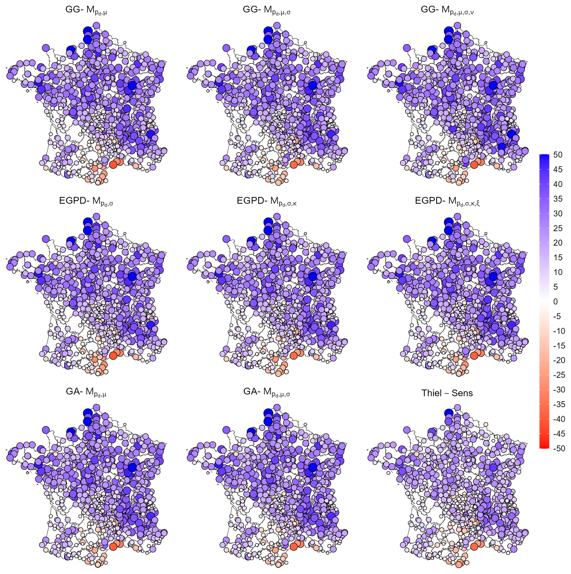
Figure A1 Maps of relative trends (%) in mean all-day precipitation (m_t for various nonstationary models and the Theil-Sen benchmark. Top row: GG models. Second row: EGPD models. Bottom row (first two maps): GA models. Bottom-right map: Trends obtained using the nonparametric Theil-Sen slope estimator (benchmark).

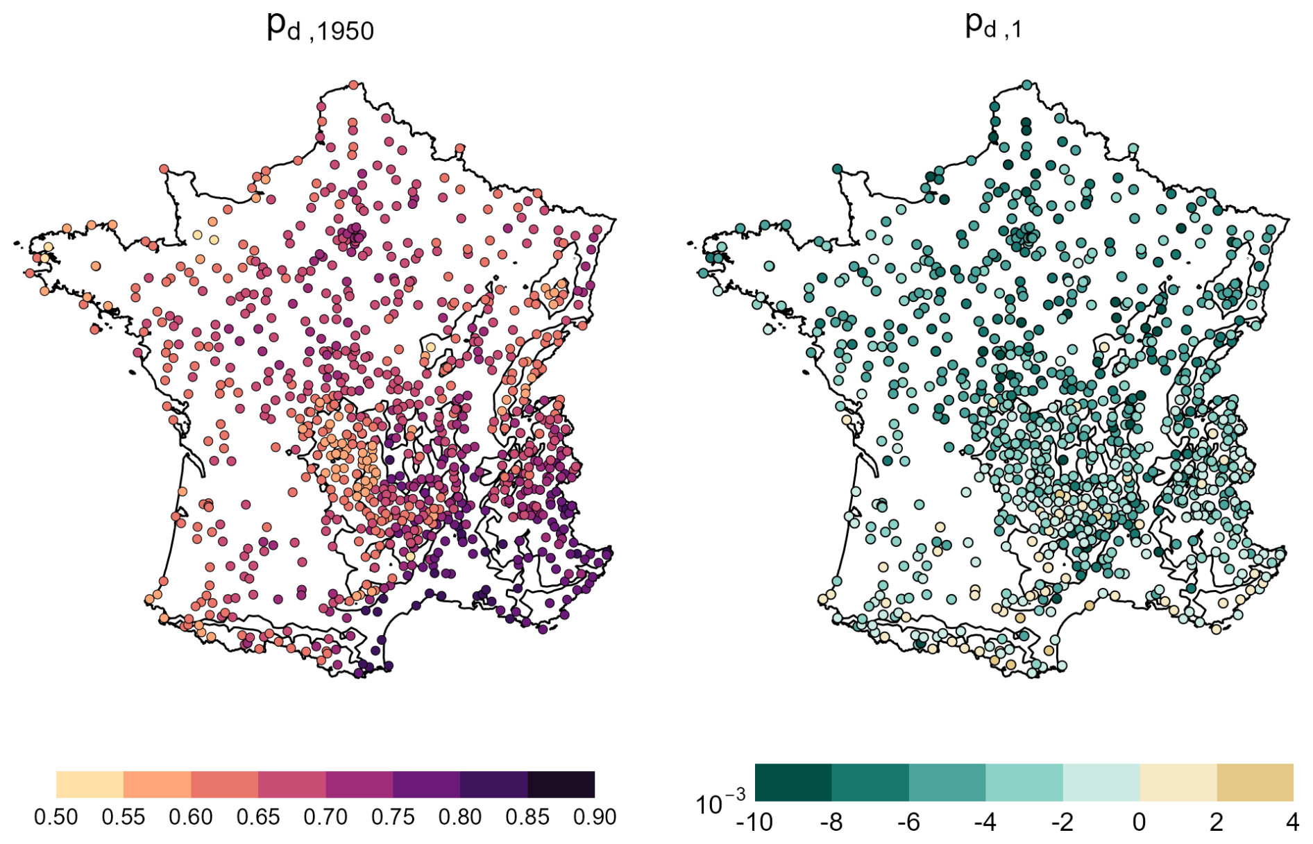
Figure A2 Dry-day component parameters from the logit model.

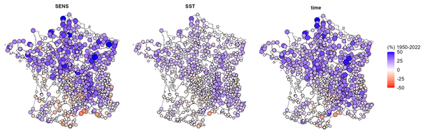
Figure A3 Changes in Wet-day frequency (1−p_d) in autumn using Sen’s slope (reference, left), and two regression models with SST (center) and time (right) as covariates.

Appendix B: Shape parameters

Figure B1 shows the map of shape parameters obtained with GEV and the nonstationary EGPD and GG (ξ₀ and ν₀ in EGPD-${\mathcal{M}}_{p_{\mathrm{d}},\mathit{\sigma },\mathit{\kappa },\mathit{\xi }}$ and GG-${\mathcal{M}}_{p_{\mathrm{d}},\mathit{\mu },\mathit{\sigma },\mathit{\nu }}$ respectively). In the case of GEV and EGPD, the tail is heavy when ξ>0, light when ξ=0 and bounded when ξ<0. For GG, the tail is heavy when ν<1, gamma like when ν=1, and lighter than gamma when ν>1.

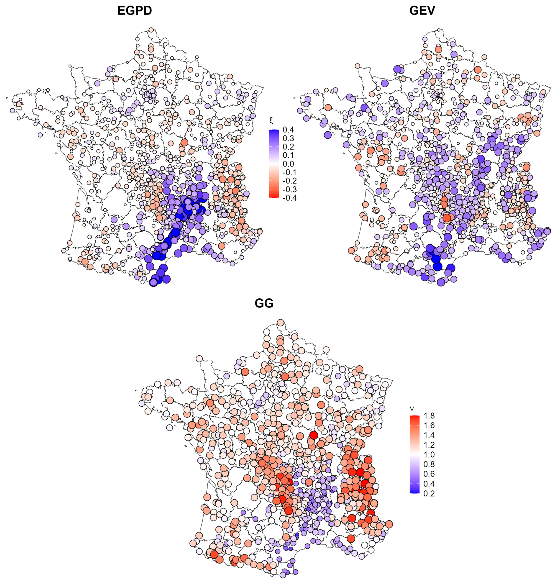
Figure B1 Map of upper tail shape parameters obtained with GEV and the nonstationary EGPD and GG (ξ₀ and ν₀ in EGPD-${\mathcal{M}}_{p_{\mathrm{d}},\mathit{\sigma },\mathit{\kappa },\mathit{\xi }}$ and GG-${\mathcal{M}}_{p_{\mathrm{d}},\mathit{\mu },\mathit{\sigma },\mathit{\nu }}$ respectively). Red color shows locations with bounded tails, blue colors show heavy tails, while light tails are shown in white.