Bivariate Gaussian models for wind vectors in a distributional regression framework

A new probabilistic post-processing method for wind vectors is presented in a distributional regression framework employing the bivariate Gaussian distribution. In contrast to previous studies, all parameters of the distribution are simultaneously modeled, namely the location and scale parameters for both wind components and also the correlation coefficient between them employing flexible regression splines. To capture a possible mismatch between the predicted and observed wind direction, ensemble forecasts of both wind components are included using flexible two-dimensional smooth functions. This encompasses a smooth rotation of the wind direction conditional on the season and the forecasted ensemble wind direction.

The performance of the new method is tested for stations located in plains, in mountain foreland, and within an alpine valley, employing ECMWF ensemble forecasts as explanatory variables for all distribution parameters. The rotation-allowing model shows distinct improvements in terms of predictive skill for all sites compared to a baseline model that post-processes each wind component separately. Moreover, different correlation specifications are tested, and small improvements compared to the model setup with no estimated correlation could be found for stations located in alpine valleys.

1 Introduction

Accurate forecasts of wind speed and direction are of great importance for decision-making processes and risk management in today's society and will likely become more important in the future. This is not only because of the rapid change in climate and the resulting increase in severe storms (e.g., Kunkel et al., 2012; Vose et al., 2013), but is also due to the change in the society itself and its technical revolution. As an example, the European Union is aiming to increase the amount of wind energy by 2030 to 35 %, which would be more than double the capacity installed at the end of 2016 (WindEurope, 2017). In the field of aviation and air traffic control for instance, more flexible landing procedures with a so-called time-based separation are currently being tested at Heathrow Airport and are planned to go operational in the near future (EuropeanCommission, 2018). In both cases, wind (power) forecasts are of fundamental importance; probabilistic wind forecasts are in particular advisable as they permit optimal risk assessment and decision making (Gneiting, 2008).

Probabilistic weather forecasts are usually issued in the form of ensemble predictions. To account for the underlying uncertainty in the atmosphere, numerical ensemble prediction systems (EPSs) provide a set of weather forecasts using slightly perturbed initial conditions and different model parameterizations (Palmer, 2002). Despite recent advances in the development of EPSs, the resulting forecasts still often show displacement errors and usually capture only part of the forecast uncertainty, especially when comparing EPS forecasts and point measurements (Buizza et al., 2005; Gneiting and Katzfuss, 2014). This often results from structural model deficiencies and insufficient resolution or unresolved topographical features. To remove systematic biases and to provide corrected variance information, statistical post-processing methods are often employed. For wind, various ensemble post-processing methods have been proposed over the last decade, mainly focusing on wind speed. For a single location, parametric examples are non-homogeneous regression (Thorarinsdottir and Gneiting, 2010; Lerch and Thorarinsdottir, 2013; Baran and Lerch, 2015, 2016), kernel dressing methods with similarities to Bayesian model averaging (Sloughter et al., 2010; Courtney et al., 2013; Baran, 2014), and extended logistic regression (Messner et al., 2014a, b). A non-parametric approach based on quantile regression forests was applied by Taillardat et al. (2016). On a regular grid, ensemble post-processing based on non-homogeneous regression was performed by Scheuerer and Möller (2015).

To account for the circular characteristics of wind or utilizing information of wind speed and direction, an intuitive post-processing approach is to model a bivariate process for the zonal and meridional wind components. Gneiting et al. (2008) suggested using a bivariate Gaussian response distribution for the wind components, an idea that was implemented by Pinson (2012). He estimates a dilation and translation factor for the individual ensemble members utilizing the empirical correlation structure of the EPS. This procedure can be seen as a variant of the ensemble copula coupling (ECC) method introduced by Schefzik et al. (2013). With the ECC, both wind components are calibrated with univariate approaches and a discrete sample drawn from each univariate predictive distribution is rearranged in the rank order structure of the raw ensemble. The method introduced by Schuhen et al. (2012) also fits a bivariate Gaussian distribution for the wind components; however, in their approach the post-processed probabilistic forecast consists of a fully specified predictive distribution instead of a discrete ensemble. As their analyses show that the observed correlation between the two wind components mainly depends on wind direction, they model the correlation parameter in the bivariate Gaussian distribution as a trigonometric function of the ensemble mean wind direction. An extra group is formed for cases with low wind speeds unconditionally on their wind direction. The estimation of the correlation parameter is done offline in a pre-processing step for a separate year, either for all stations combined or for each station individually. However, according to Schuhen et al. (2012), the fitting can be critical for individual stations since wind sectors may only contain a few data points.

For stations in complex terrain, a possible drawback of the bivariate post-processing approach of Schuhen et al. (2012) is that the model cannot correct for a systematic distortion in the wind directions due to discrepancies between the model and real topography. Especially when the respective valley orientations differ, a meridional wind component might be partially rotated into a zonal wind component and vice versa. Pinson (2012) employs both forecasted wind components for the calibration of the zonal or meridional wind component, which is partly able to correct for systematic distortions in wind directions in a linear manner. In the field of post-processing deterministic weather forecasts, this approach was already suggested by Glahn and Lowry (1972).

Alternatively to bivariate calibration methods, wind direction can also be employed in univariate settings. In a post-processing approach for wind speed, Eide et al. (2017) suggest utilizing the potentially nonlinear information of the wind direction by a generalized additive model (GAM; Hastie and Tibshirani, 1986). GAMs were first applied in the meteorological context by Vislocky and Fritsch (1995) and provide a powerful statistical model framework which can capture potential nonlinear relationships between the covariates and the response by smooth functions or splines. Eide et al. (2017) employ wind direction as an additional covariate for the estimation of wind speed, by accounting for its cyclic and potential nonlinear characteristics utilizing thin-plate regression splines.

In this study, we directly model the zonal and meridional wind components, employing the bivariate Gaussian distribution as suggested by Gneiting et al. (2008) and performed by Pinson (2012) and Schuhen et al. (2012). However, we capture all distribution parameters, namely the location and scale parameters for both wind components, and also the correlation coefficient between them in a single flexible model. In the estimation of the two-dimensional location and scale parameters the information value of both ensemble wind components is utilized to allow for a smooth rotation of the forecasted wind direction accounting for unresolved topographical features. To consider the correlation characteristics detected in Schuhen et al. (2012) and to allow for possible nonlinear effects, such as, e.g., suggested by Eide et al. (2017), we model the correlation as a function of wind speed and direction utilizing cyclic regression splines. To account for potential time-varying effects, all linear predictors use a time-adaptive intercept and time-adaptive slope coefficients based on cyclic smooth splines.

The paper is structured as follows: Sect. 2 introduces the employed statistical models. The underlying data of this study are shortly described in Sect. 3. Within Sect. 4, first a model comparison and validation are presented for two weather stations with different site characteristics, followed by aggregated scores for station sites located in plains, in mountain foreland, and within an alpine valley. The article ends with a brief discussion and a conclusion given in Sect. 5.

2 Methods

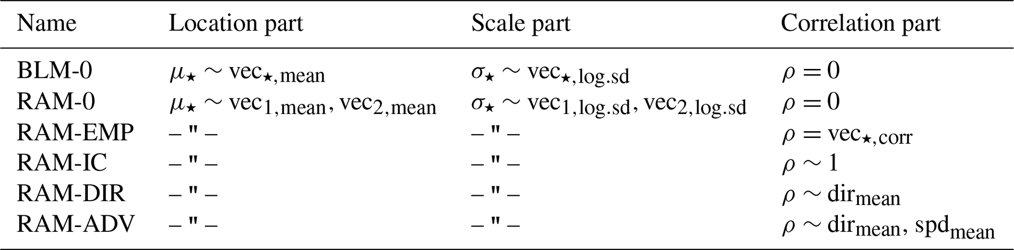
In Sect. 2.1, the bivariate Gaussian distribution is reviewed and briefly presented in a distributional regression framework. Subsequently, three broad model classes are introduced, all of which are based on a time-adaptive training scheme but employ different specifications for the location, scale, and correlation parameters of the bivariate distribution. First, the baseline model is presented in Sect. 2.2 that serves as a benchmark and simply combines two univariate heteroscedastic regression models that post-process each wind component separately. Second, the baseline model is extended in Sect. 2.3 by always adding both EPS wind components as regressors using smooth splines and thus allowing for potential misspecifications in the EPS wind direction. Finally, Sect. 2.4 also considers models with estimated correlation coefficients based on various regression specifications. Table 1 provides a synoptic summary of all bivariate Gaussian model specifications tested within this study.

Table 1 Overview of bivariate Gaussian model specifications. For the “baseline model” (BLM-0; see Sect. 2.2) and the “rotation-allowing model” (RAM-0; see Sect. 2.3) no correlation is employed, i.e., fixed at zero. For all tested correlation specifications, the RAM-0 setup is employed for the location and scale part (see Sect. 2.4). In all setups for each distribution parameter, a seasonally varying intercept effect is estimated. For BLM-0, a seasonally varying slope coefficient is fitted for the two wind components in the location and scale parts. For the RAM-0 setup, the slope coefficients are additionally dependent on the wind direction. In the RAM-ADV correlation model, the wind speed is modeled conditional on the wind direction. The equal sign expresses “the response is set to” and the tilde signals “the response is modeled by” the term(s) on the right-hand side of the equation. The symbol “– " –” implies that the same configuration as in the line above is employed.

2.1 Distributional regression for a bivariate Gaussian response

The zonal and meridional components of the horizontal wind vector are represented by a bivariate Gaussian distribution. Its likelihood function L is given by

$$\begin{array}{}\text{(1)}& \begin{array}{rl}& L(\mathit{\mu },\mathbf{\Sigma }|\mathit{y})=\\ & {\displaystyle \frac{\mathrm{1}}{\sqrt{\left(\mathrm{2}\mathit{\pi }{)}^{\mathrm{2}}\right|\mathbf{\Sigma }|}}}\exp \left(-{\displaystyle \frac{\mathrm{1}}{\mathrm{2}}}(\mathit{y}-\mathit{\mu }{)}^{\top }{\mathbf{\Sigma }}^{-\mathrm{1}}(\mathit{y}-\mathit{\mu })\right),\end{array}\end{array}$$

where $\mathit{y}=(y_{\mathrm{1}},y_{\mathrm{2}}{)}^{\top }$ are bivariate observations and $\mathit{\mu }=({\mathit{\mu }}_{\mathrm{1}},{\mathit{\mu }}_{\mathrm{2}}{)}^{\top }$ are the distributional location parameters with ${\mathit{\mu }}_{\star }\in \mathbb{R}$; the subscript asterisk acts as a placeholder for the zonal and meridional wind components from here on. The covariance matrix is defined as

$$\begin{array}{}\text{(2)}& \mathbf{\Sigma }=\left(\begin{array}{cc}{\mathit{\sigma }}_{\mathrm{1}}^{\mathrm{2}}& \mathit{\rho }{\mathit{\sigma }}_{\mathrm{1}}{\mathit{\sigma }}_{\mathrm{2}}\\ \mathit{\rho }{\mathit{\sigma }}_{\mathrm{1}}{\mathit{\sigma }}_{\mathrm{2}}& {\mathit{\sigma }}_{\mathrm{2}}^{\mathrm{2}}\end{array}\right),\end{array}$$

with correlation parameter $\mathit{\rho }\in [-\mathrm{1},\mathrm{1}]$ and scale parameters ${\mathit{\sigma }}_{\star }>\mathrm{0}$. In the framework of distributional regression, link functions provide the relationship between unrestricted linear predictors and the respective distribution parameters by ensuring their appropriate co-domain. For the bivariate Gaussian distribution, the location parameters μ_⋆, the scale parameters σ_⋆, and the correlation parameter ρ are linked to their additive predictors by an identity, logarithm and rhogit link, respectively (Klein et al., 2014).

To be able to utilize the information of cyclic covariates, such as, e.g., wind direction in addition to linear covariates, we follow Eide et al. (2017) and fit a GAM but utilize cubic smooth functions with cyclic constraints for all cyclic covariates (Wood, 2017; see Appendix A1). In the context of distributional regression, additive models with smooth effects are typically referred to as “generalized additive models for location, scale and shape” (GAMLSS, Rigby and Stasinopoulos, 2005). In this study, we utilize GAMLSS in a Bayesian framework, which allows us to examine the estimated effects based on Markov chain Monte Carlo (MCMC) simulations and ensures stable estimation of the regression coefficients. The key steps involved in the estimation can be summarized as follows. The parameters of the bivariate Gaussian distribution are linked to the set of additive predictors containing potentially nonlinear transformations of the covariates according to the model specifications described later on in this section. The model fitting is performed by a derivative-based MCMC sampling using iteratively weighted least squares (IWLS, Gamerman, 1997) proposals. Hence, the estimated effects are based on 1000 independent realizations of the regression coefficients drawn from the Markov chains and for subsequent predictions the means of these samples are used as point estimators for the regression coefficients. A comprehensive summary of the method is given in Umlauf et al. (2018).

2.2 Baseline model (BLM-0)

The baseline model (BLM-0) combines two univariate heteroscedastic regression models that post-process each wind component separately with correlation fixed at zero. Hence, for the location and scale part, it uses its direct counterparts of the EPS as covariates, namely EPS-forecasted zonal wind information (vec₁) to model the zonal component of the bivariate response and EPS-forecasted meridional wind information (vec₂) to model the meridional component:

$$\begin{array}{}\text{(3)}& {\displaystyle }\begin{array}{rl}& {\mathit{\mu }}_{\star }=\underset{\mathrm{intercept}}{\underbrace{{{\mathit{\alpha }}_{\star }}_{\mathrm{0}}+{f_{\star }}_{\mathrm{0}}\left(\mathrm{doy}\right)}}+\underset{\mathrm{slope}\mathrm{coefficient}}{\underbrace{({{\mathit{\alpha }}_{\star }}_{\mathrm{1}}+{f_{\star }}_{\mathrm{1}}(\mathrm{doy}\left)\right)}}\cdot {\mathrm{vec}}_{\star ,\mathrm{mean}},\\ & \log \left({\mathit{\sigma }}_{\star }\right)=\underset{\mathrm{intercept}}{\underbrace{{{\mathit{\beta }}_{\star }}_{\mathrm{0}}+{g_{\star }}_{\mathrm{0}}\left(\mathrm{doy}\right)}}+\underset{\mathrm{slope}\mathrm{coefficient}}{\underbrace{({{\mathit{\beta }}_{\star }}_{\mathrm{1}}+{g_{\star }}_{\mathrm{1}}(\mathrm{doy}\left)\right)}}\cdot {\mathrm{vec}}_{\star ,\log .\mathrm{sd}},\end{array}\end{array}$$

where α_• and β_• are regression coefficients, and f_•(doy) and g_•(doy) employ cyclic regression splines conditional on the day of the year (doy). The subscripts mean and log.sd refer to the mean and log standard deviation of the ensemble wind components, respectively. We follow Gebetsberger et al. (2017) and use the logarithm transformation for the standard deviation of the ensemble members to ensure positivity, which is preferable for the estimation process.

Equation (3) specifies a time-adaptive training scheme (with further details in Appendix A2), where the linear predictors consist of a global intercept and slope coefficient plus a seasonally varying deviation. Thus, the intercept and slope coefficients can smoothly evolve over the year in case the bias or the covariate's skill varies seasonally. If there is no seasonal variation, the nonlinear effects become zero and Eq. (3) simplifies to a regression model with a constant intercept and slope coefficient (${\mathit{\mu }}_{\star }={{\mathit{\alpha }}_{\star }}_{\mathrm{0}}+{{\mathit{\alpha }}_{\star }}_{\mathrm{1}}\cdot {\mathrm{vec}}_{\star ,\mathrm{mean}}$; $\log \left({\mathit{\sigma }}_{\star }\right)={{\mathit{\beta }}_{\star }}_{\mathrm{0}}+{{\mathit{\beta }}_{\star }}_{\mathrm{1}}\cdot {\mathrm{vec}}_{\star ,\log .\mathrm{sd}}$).

2.3 Rotation-allowing model without correlation (RAM-0)

In the second model, labeled the rotation-allowing model (RAM-0), we extend the BLM-0 setup by employing the zonal and meridional wind information of the ensemble for the linear predictors of all location and scale parameters. That means we use the ensemble information of both the zonal and meridional wind components for the two components of the response (cf. Glahn and Lowry, 1972). In case of a perfect EPS the zonal wind predictions are non-informative covariates for the meridional wind component and vice versa. However, if, e.g., the model topography is not sufficiently resolved or in the case of local shadowing effects, both EPS wind components may contain valuable information for the zonal and meridional wind components of the response. Especially in a mountain valley, when the model and real valley orientation differs, both wind components of the ensemble can potentially contain information about both location and scale parameters, respectively. Thus, we propose to employ seasonally varying effects depending on the ensemble wind direction, which allows the model to rotate the forecasted wind direction if necessary. To do so, we obtain a two-dimensional smooth function represented by a tensor product spline with a respective cyclic constraint for the day of the year (doy) and for the mean ensemble wind direction (dir_mean):

$$\begin{array}{}\text{(4)}& \begin{array}{rl}& {\mathit{\mu }}_{\star }={{\mathit{\alpha }}_{\star }}_{\mathrm{0}}+{f_{\star }}_{\mathrm{0}}\left(\mathrm{doy}\right)\\ & +\left({{\mathit{\alpha }}_{\star }}_{\mathrm{1}}+{f_{\star }}_{\mathrm{1}}\left(\mathrm{doy}\right)\cdot {f_{\star }}_{\mathrm{2}}\left({\mathrm{dir}}_{\mathrm{mean}}\right)\right)\cdot {\mathrm{vec}}_{\mathrm{1},\mathrm{mean}}\\ & +\left({{\mathit{\alpha }}_{\star }}_{\mathrm{2}}+{f_{\star }}_{\mathrm{3}}\left(\mathrm{doy}\right)\cdot {f_{\star }}_{\mathrm{4}}\left({\mathrm{dir}}_{\mathrm{mean}}\right)\right)\cdot {\mathrm{vec}}_{\mathrm{2},\mathrm{mean}},\\ & \log \left({\mathit{\sigma }}_{\star }\right)={{\mathit{\beta }}_{\star }}_{\mathrm{0}}+{g_{\star }}_{\mathrm{0}}\left(\mathrm{doy}\right)\\ & +\left({{\mathit{\beta }}_{\star }}_{\mathrm{1}}+{g_{\star }}_{\mathrm{1}}\left(\mathrm{doy}\right)\cdot {g_{\star }}_{\mathrm{2}}\left({\mathrm{dir}}_{\mathrm{mean}}\right)\right)\cdot {\mathrm{vec}}_{\mathrm{1},\log .\mathrm{sd}}\\ & +\left({{\mathit{\beta }}_{\star }}_{\mathrm{2}}+{g_{\star }}_{\mathrm{3}}\left(\mathrm{doy}\right)\cdot {g_{\star }}_{\mathrm{4}}\left({\mathrm{dir}}_{\mathrm{mean}}\right)\right)\cdot {\mathrm{vec}}_{\mathrm{2},\log .\mathrm{sd}},\end{array}\end{array}$$

where, as before, α_• and β_• are regression coefficients, and f_• and g_• employ cyclic regression splines. From a more physical perspective, the two-dimensional smooth effects rotate the ensemble wind components conditional on the day of the year and the ensemble wind direction.

2.4 Rotation-allowing models with correlation

By explicitly modeling the correlation, we further extend the RAM-0 setup within this section. For the estimation of the correlation structure different model specifications are tested. The most advanced specification, RAM-ADV, assumes that the correlation mainly depends on the mean ensemble wind direction (dir_mean) and speed (spd_mean) by modeling a linear interaction between these two covariates:

$$\begin{array}{}\text{(5)}& {\displaystyle }\begin{array}{rl}\mathrm{rhogit}\left(\mathit{\rho }\right)& ={\mathit{\gamma }}_{\mathrm{0}}+h_{\mathrm{0}}\left(\mathrm{doy}\right)+h_{\mathrm{1}}\left({\mathrm{dir}}_{\mathrm{mean}}\right)\\ & +({\mathit{\gamma }}_{\mathrm{1}}+h_{\mathrm{2}}({\mathrm{dir}}_{\mathrm{mean}}\left)\right)\cdot {\mathrm{spd}}_{\mathrm{mean}},\end{array}\end{array}$$

with $\mathrm{rhogit}\left(\mathit{\rho }\right)=\mathit{\rho }/\sqrt{(\mathrm{1}-{\mathit{\rho }}^{\mathrm{2}})}$; γ₀ is the global intercept and h₀(doy) the seasonally varying intercept. The effect h₁(dir_mean) estimates the dependence of the correlation given the wind direction and $({\mathit{\gamma }}_{\mathrm{1}}+h_{\mathrm{2}}({\mathrm{dir}}_{\mathrm{mean}}\left)\right)\cdot {\mathrm{spd}}_{\mathrm{mean}}$ employs a varying effect of wind speed conditional on the wind direction. The estimation of the underlying correlation structure is in accordance with results of Schuhen et al. (2012), who employ wind direction and an offset of wind speed as informative covariates in the estimation of the correlation parameter.

Other implementations tested for the correlation parameter are an intercept-only model (RAM-IC), a model with a cyclic effect solely depending on wind direction (RAM-DIR), the RAM-0 independent-component model (Sect. 2.3), and a model using the empirical correlation (corr) of the raw ensemble (RAM-EMP). A synoptic table of all models tested in this study is given in Table 1.

3 Data

3.1 Observational data

The validation and comparison of the different model specifications are performed for 15 measurement sites located across Austria, Germany, and Switzerland. The sites are chosen to investigate the influence of different underlying topographies or varying discrepancies between the real and model topography on the post-processing. The stations are divided into three groups representing sites located in plains, mountain foreland, and within an alpine valley. An overview of the stations is given in Fig. 1. The results for stations Hamburg and Innsbruck, which are labeled in Fig. 1, are discussed in more detail in Sect. 4. At all meteorological sites, wind speed and direction measurements are reported for the 10 m height level. The data are 10 min averages for the period 26 January 2010 to 7 March 2016, yielding a total of 2233 d.

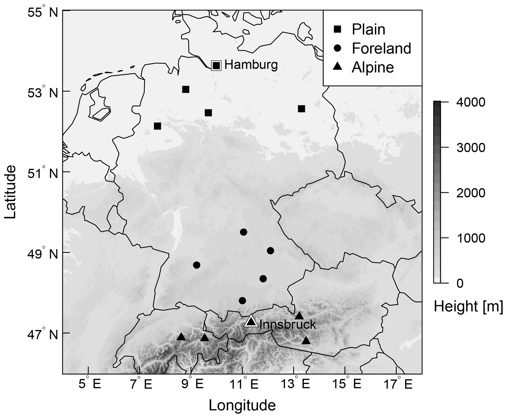
Figure 1 Overview of the study area with selected stations classified as plain, foreland, and alpine station sites. The labeled stations with a white background, Hamburg and Innsbruck, are discussed in detail in Sect. 4. Elevation data are obtained from the SRTM-30 m digital elevation model (NASA JPL, 2013).

3.2 Ensemble prediction system

Covariates are derived from the global 50-member EPS of the European Centre for Medium-Range Weather Forecasts (ECMWF). These EPS forecasts have a horizontal resolution of approximately 30 km (T639) for the time between January 2010 and March 2016 and are bilinearly interpolated to the measurement sites. Covariates employed in this study are the zonal and meridional wind components as well as the derived quantities wind speed and direction valid at 10 m above ground. For all these variables, two statistics are computed over the 50 perturbed ensemble members, namely the mean and the logarithm of the standard deviation (log.sd). Additionally, the Pearson sample correlation coefficient (corr) is computed from the raw ensemble members to capture the correlation between the two wind components. Forecasts are taken from the EPS run initialized at 00:00 UTC for forecast steps ranging from +12 to +72 h ahead at a 12-hourly temporal resolution. Figure 2 shows the empirical wind distributions of the observed and predicted winds for Innsbruck and Hamburg for forecast steps +12 and +24 h corresponding to 12:00 and 00:00 UTC.

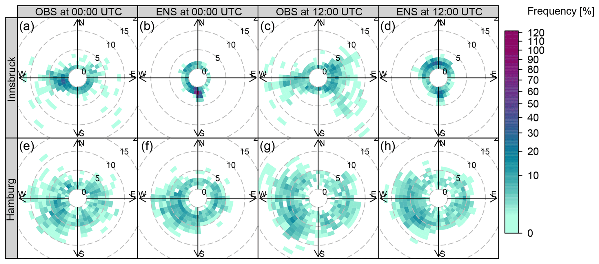
Figure 2 Empirical wind distributions of observations (OBS) and mean ensemble forecasts (ENS) for Innsbruck and Hamburg. The probability of occurrence is color-coded and the wind speed is represented by contour lines (m s⁻¹). The forecast steps +12 and +24 h, valid at 12:00 and 00:00 UTC, are shown for the validation period from 24 February 2014 to 7 March 2016.

4 Results

This section presents the results of the statistical post-processing models. The structure is as follows. First, the estimated effects of the baseline model, BLM-0 (Sect. 4.1), and the rotation-allowing model, RAM-0 (Sect. 4.2), are shown for two stations representative of one alpine valley site and of a measurement site in the plains. For both models a constant correlation of zero is employed, and their predictive performance is discussed in Sect. 4.3. Afterwards, model comparison (Sect. 4.4) and validation (Sect. 4.5) of the different correlation specifications are given for the two representative stations. In Sect. 4.6, the overall performance of the model setups is evaluated for three groups of stations classified as topographically plain, mountain foreland, and alpine valley sites.

The model estimation is performed on data of the first 4 years, leaving an out-of-sample validation data set ranging from 24 February 2014 to 7 March 2016.

4.1 Baseline model (BLM-0)

For BLM-0, the cyclic seasonal effects for stations Hamburg and Innsbruck are shown in Fig. 3 as solid and dashed lines with the respective 95 % credible intervals. The estimated effects are on the scale of the additive predictor, i.e., on the linear scale for the location parameters μ_⋆ and on the log scale for the scale parameters σ_⋆. Each of the four distribution parameters is described by a (potentially) seasonally varying effect for the intercept (panels a, c, e and g) and the slope coefficient (panels b, d, f and h) as specified in Eq. (3).

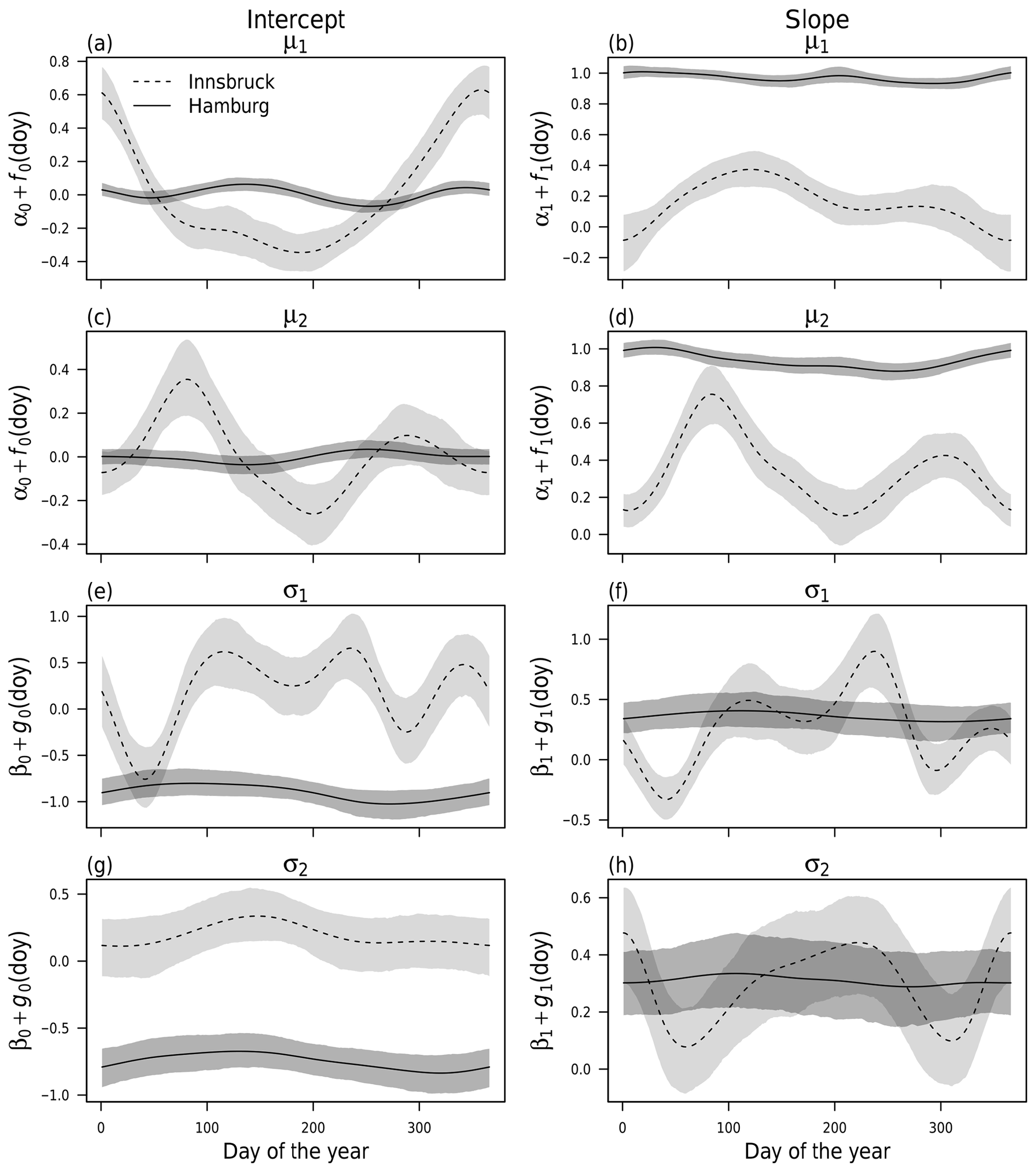
Figure 3 Cyclic seasonal intercept and slope effects according to Eq. (3) employing a constant correlation of zero for weather stations Innsbruck (dashed) and Hamburg (solid) at forecast step +12 h (valid at 12:00 UTC). The effects for the location parameters μ_⋆ (a–d) and scale parameters σ_⋆ (e–h) are shown on the linear and log scales, respectively. The shading represents the 95 % credible intervals based on MCMC sampling.

For Hamburg, for both location parameters μ_⋆, the intercept effect is almost zero (Fig. 3a, c) and the effect for the slope coefficient is close to one (Fig. 3b, d) with very little seasonal variability. This means apparently no bias correction is necessary and the ensemble mean wind components are mapped almost one-to-one to the location parameters. Similarly, barely any seasonal variation exists for the scale parameters σ_⋆ (Fig. 3e–h); however, here the intercept and slope coefficients actually post-process the EPS variances of the wind components (rather than a one-to-one mapping only), leading to an increase in the scale parameters compared to the under-dispersed ensemble. The 95 % credible intervals indicate a higher uncertainty of the estimated scale parameters compared to the location parameters. In summary, the EPS performance for Hamburg is almost constant over the year, and no time-adaptive training scheme seems to be necessary.

By contrast, for Innsbruck the estimated effects show a distinct annual cycle for the location parameters μ_⋆, which indicates a varying information content of the predictor variables ${\mathrm{vec}}_{\star ,\mathrm{mean}}$ and the need for some adaptive training scheme. For the location parameter μ₁, the intercept is rather large during winter (Fig. 3a), while, at the same time, the slope coefficient (Fig. 3b) is close to zero due to an apparently low skill of the EPS. For the location parameter μ₂ (Fig. 3c, d), the higher slope coefficients during spring and autumn suggest a higher information content of the raw EPS in the transitional seasons than for the rest of the year. For the scale parameters (Fig. 3e–h), the estimated effects show high variability; this indicates a seasonally varying skill of the EPS variance information. In summary, for the weather station in Innsbruck, the information content of the ensemble wind predictions seems to be rather low. This is in accordance with the clearly different pattern of observations and EPS forecasts shown in Fig. 2.

4.2 Rotation-allowing model without correlation (RAM-0)

Figure 4 shows the estimated mean effects of the RAM-0 setup in comparison with BLM-0 on the wind direction at Innsbruck and Hamburg for the forecast steps +12 and +24 h valid at 12:00 and 00:00 UTC, respectively. The marginal effects are non-centered and shown for the mean covariates within 10^∘ wind sectors conditional on the day of the year. The BLM-0 model for Innsbruck shows a distinct seasonal dependency of the post-processed wind direction for both times of the day (Fig. 4a, c). During winter at 12:00 and 00:00 UTC, mainly down-valley winds (approximately 280^∘) are predicted, whereas over the rest of the year, the EPS mainly forecasts up-valley wind directions. This pattern is more pronounced during night (00:00 UTC) and has less variability in summer. In general, the BLM-0 setup seems to mainly capture the climatological mean wind direction; this leads to little variations between the different wind directions issued by the EPS. In contrast, the rotation-allowing RAM-0 setup has the flexibility to post-process the wind directions conditional on the forecasted EPS wind direction, which is apparent for the Innsbruck station at both 12:00 and 00:00 UTC: for 12:00 UTC the seasonal dependency leads to either up-valley or down-valley wind conditional on the ensemble wind direction and on the day of the year (Fig. 4b), whereas at 00:00 UTC almost no seasonal variation exists and the predicted wind direction solely depends on the issued ensemble wind forecasts (Fig. 4d). At Hamburg, a completely different picture can be seen: almost no post-processing conditional on the ensemble wind direction or the day of the year is visible for both time steps and model setups (Fig. 4e–f). In other words, the predicted ensemble wind direction fits the observed wind direction quite well, and only little statistical correction is needed.

Figure 4 Estimated mean effects for the derived post-processed wind direction at Innsbruck (a–d) and Hamburg (e–h) for the forecast steps +12 and +24 h (valid at 12:00 and 00:00 UTC). The colored lines show marginal effects for the post-processed wind direction conditional on mean values within 10^∘ wide wind sectors given the training data set. The effects are non-centered and are calculated conditional on the day of the year according to model setups BLM-0 (a, c, e, g; Eq. 3) and RAM-0 (b, d, f, h; Eq. 4).

4.3 Predictive performance – models without correlation

To investigate the predictive performance of the two competing setups, Fig. 5 shows the discretized logarithmic score based on the bivariate Gaussian distribution (LS; see Appendix B) and the energy score (ES; see Appendix B) for the forecast steps from +12 to +72 h at a 12-hourly temporal resolution. In addition, skill scores are shown with the raw EPS as a reference or comparing the different setups to each other. Both multivariate scores are proper scores (Gneiting and Raftery, 2007) and evaluate the full predictive distribution returned by the statistical models. The scores for the different forecast horizons show an overall better predictive performance at Hamburg than at Innsbruck. For both stations, the forecasts valid at 00:00 UTC have more skill than those for 12:00 UTC, with higher diurnal variations at Innsbruck. In terms of the ES, the improvements of the BLM-0 model over the raw EPS are about 29 % for Innsbruck and 8 % for Hamburg (Fig. 5e, f). In terms of the LS (Fig. 5b, c), the skill scores are higher, with improvements of approximately 87 % and 33 % for Innsbruck and Hamburg, respectively. The predictive performance gain for the more flexible rotation-allowing RAM-0 setup compared to the BLM-0 specification is around 7 % for Innsbruck and 2 % for Hamburg in terms of the ES (Fig. 5e, f). The LS shows slightly less pronounced relative improvements for the more flexible setup (4 % and 1 %; Fig. 5b, c). The distinct improvements in the scores for RAM-0 are as expected for Innsbruck due to a more flexible utilization of the ensemble information. For plain areas like Hamburg, we assume the better performance is based on an enhanced adjustment of the location parameters as both wind components are included in the linear predictors and is not due to the smooth rotation (cf. Fig. 4).

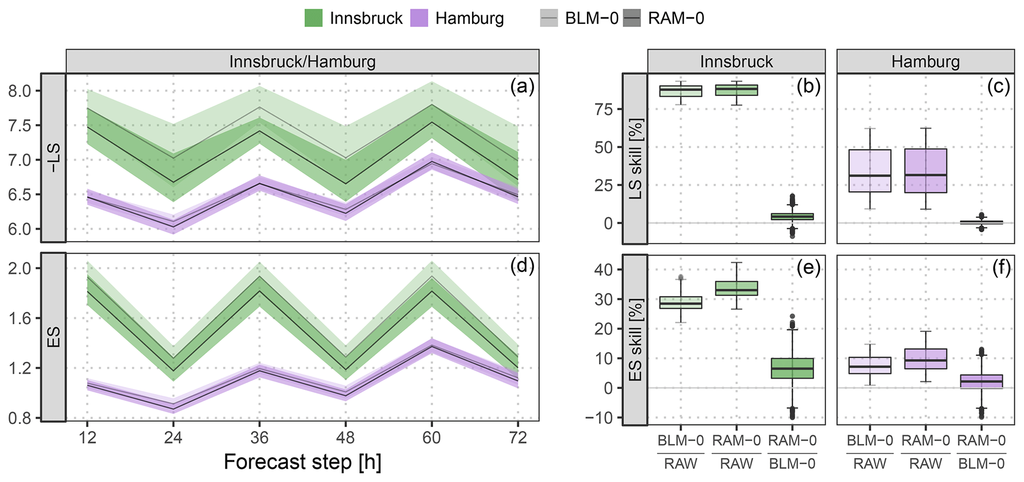
Figure 5 Predictive performance in terms of the logarithmic score (LS) and the energy score (ES) based on the full predictive bivariate distribution for the out-of-sample validation period. The two specifications BLM-0 (Eq. 3) and RAM-0 (Eq. 4) are compared. (a, d) Evolution over time for the forecast steps from +12 to +72 h at a 12-hourly temporal resolution. The solid lines represent the mean values per forecast step, the shading the respective 95 % confidence intervals based on boot-strapped mean values. To unify the orientation of both scores, the negative LS is shown (i.e., smaller is better). (b, c, e, f) Aggregated skill scores over the forecast steps, comparing the specifications BLM-0 and RAM-0 either against the raw ensemble (RAW) or against each other. Skill scores are in percent; positive values indicate improvements over the reference.

4.4 Rotation-allowing models with correlation

After investigating the two competing location or scale setups, we now focus on an extension of the RAM-0 model by explicitly estimating the underlying correlation structure. Different model specifications for the correlation parameter ρ are tested employing the same linear predictors for μ_⋆ and σ_⋆ (see Table 1).

Figure 6 shows correlation parameters predicted by different models for the forecast step +12 h for the full validation period. For comparison, the underlying correlation structure of the raw EPS is also shown. The latter is distributed similarly for Innsbruck and Hamburg and has almost the shape of a Gaussian distribution (Fig. 6a, e). The RAM-IC intercept-only model, with a varying intercept over the year, estimates correlations between −0.27 and 0.48 for Innsbruck (Fig. 6b) and values near zero without clear seasonal variations for Hamburg (Fig. 6f). At both stations, the models with varying effects conditional on the wind direction have similarly distributed correlation parameters with a slightly larger range of predicted values for the RAM-ADV model (Fig. 6d, f) than for the RAM-DIR setup (Fig. 6c, g). The predicted correlation parameters are on average larger for Innsbruck than for Hamburg.

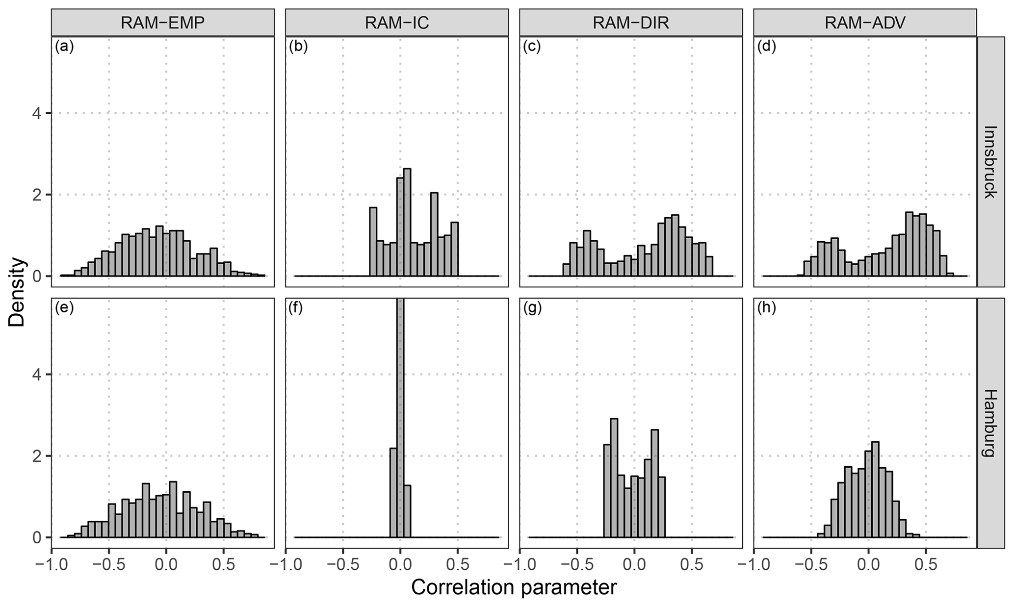
Figure 6 Distribution of the correlation parameters for the underlying dependence structure of the raw ensemble and for the fitted correlation according to the models specified in Table 1. The distributions are shown for Innsbruck (a–d) and Hamburg (e–h) at the forecast step +12 h for the out-of-sample validation period.

4.5 Predictive performance – models with correlation

Figure 7 shows the verification of bivariate wind speed predictions with an explicitly estimated correlation parameter for Innsbruck and Hamburg; the scores are aggregated over the forecast steps +12 to +72 h at a 12-hourly temporal resolution. As in Fig. 5, the predictive performance is validated in terms of the LS and the ES, based on the full predictive bivariate distributions. However, for comparing different predictive distributions with different correlation structures, the ES' discriminatory ability is limited as it mainly focuses on the location part and hardly discriminates between different correlation structures (Pinson and Tastu, 2013). In Fig. 7, skill scores are shown for the different correlation models with the RAM-0 post-processed model as a reference. The RAM-EMP model, employing the empirical correlation of the raw EPS, performs slightly worse than the reference model for both stations and both scores. This indicates that the raw dependence structure of the EPS has rather low skill. However, for all other models which explicitly model the correlation, only little additional improvement in terms of the LS and the ES is found. At Innsbruck, the RAM-IC intercept-only model performs best in terms of the ES (Fig. 7c). Regarding the LS, minor benefits are present for the most flexible model setup, RAM-ADV (Fig. 7a). For Hamburg, a similar picture is depicted in terms of the LS (Fig. 7b). For the ES (Fig. 7d), the RAM-IC model performs slightly worse than the reference model, and the RAM-ADV model setup performs best.

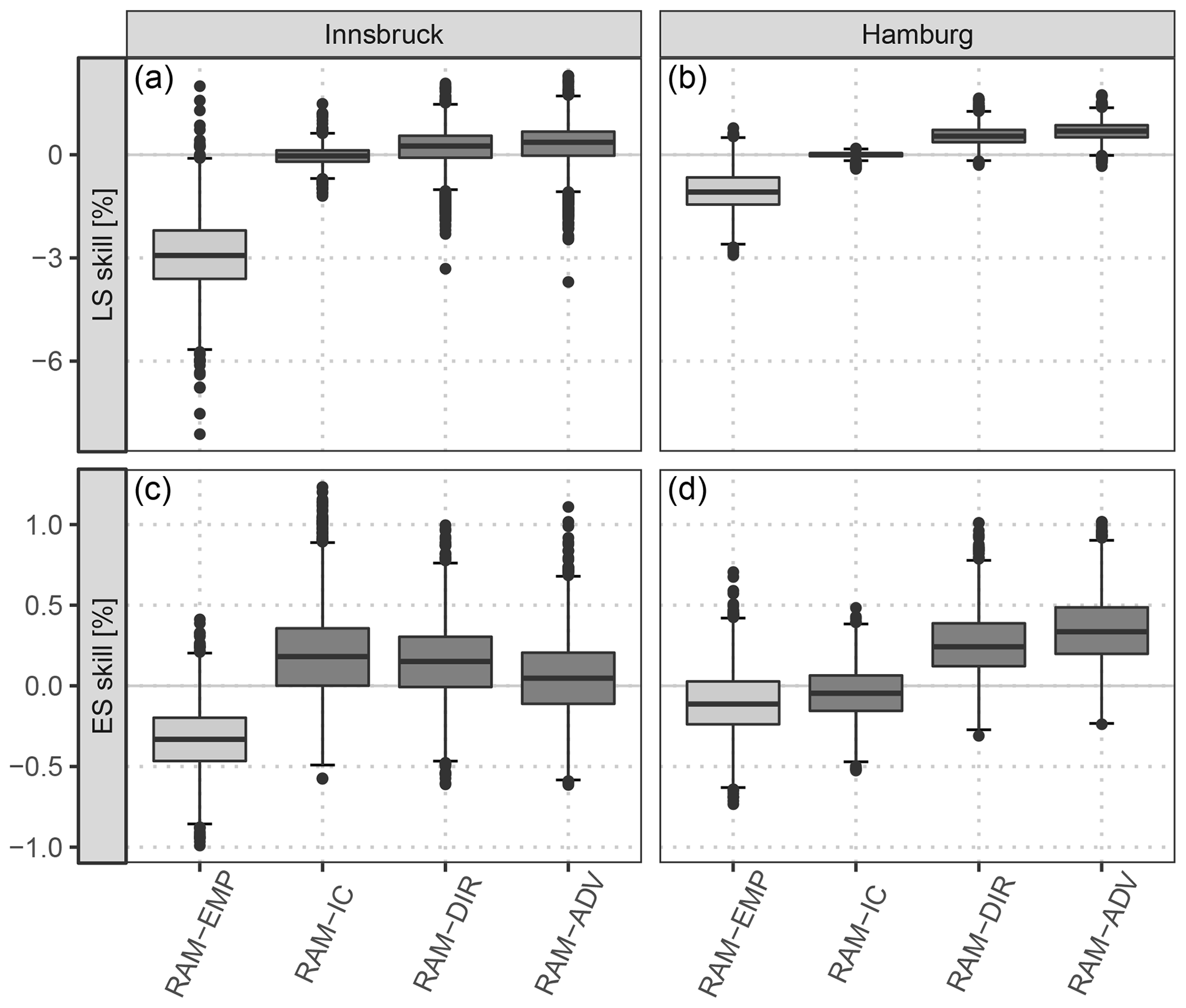
Figure 7 Skill scores aggregated over all forecast steps from +12 to +72 h at a 12-hourly temporal resolution based on the full predictive bivariate distribution for the out-of-sample validation period for Innsbruck (a, c) and Hamburg (b, d). Each box-whisker contains boot-strapped mean values per forecast step. The scores are shown for the different correlation models specified in Table 1, with the univariate post-processed model assuming a constant correlation of zero (RAM-0) as a reference. The lighter gray color for the RAM-EMP model indicates that it uses the correlation structure of the raw ensemble without further correlation. Skill scores are in percent; positive values indicate improvements over the reference.

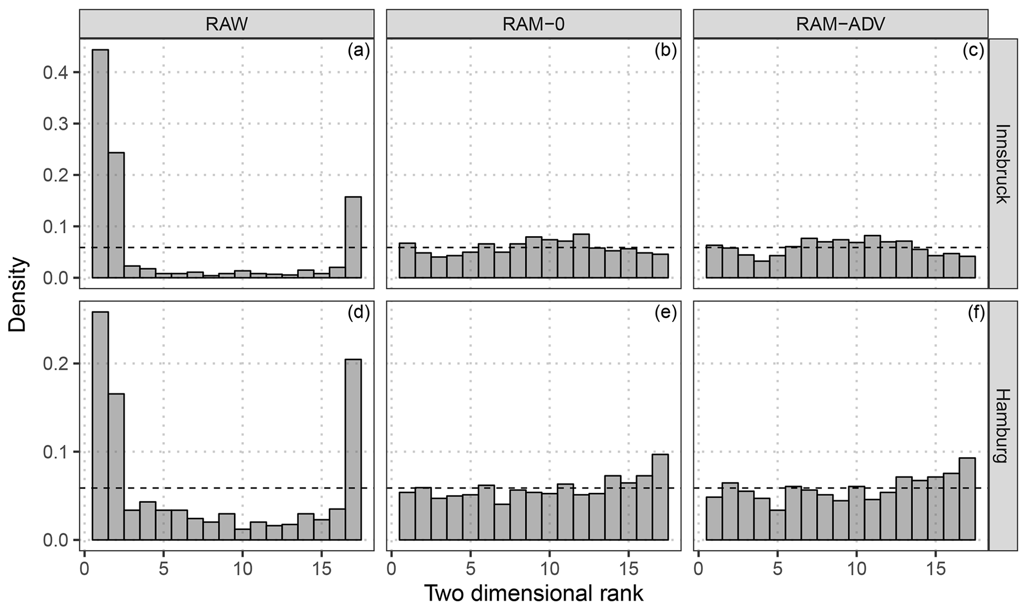
Figure 8 Multivariate rank histograms for raw and post-processed ensemble forecasts according to the correlation model setups RAM-0 and RAM-ADV. The results are shown for Innsbruck (a–c) and Hamburg (d–f) at the forecast step +12 h for the out-of-sample validation period. For purposes of presentation, three ranks of the raw EPS are combined in a single bar. To stabilize the randomness of ties in the calculation of the multivariate ranks, the median of 20 independent repetitions is plotted.

To validate the calibration of the post-processed predictions, multivariate rank histograms (Gneiting, 2008) are exemplarily shown for the model with no correlation RAM-0 and for the model with the most flexible regression splines in comparison to the raw EPS (Fig. 8). Although the latter is valid for the grid cell rather than for a single location, both model setups tested are clearly better calibrated than the highly under-dispersive raw ensemble. However, for Innsbruck the multivariate rank histograms of the post-processed forecasts are slightly over-dispersive (Fig. 8b, c) and for Hamburg slightly negatively skewed (Fig. 8e, f). The RAM-ADV flexible model setup shows no significant difference compared to the model with assumed zero correlation (RAM-0).

4.6 Evaluation for all sites

After the previous model comparison at two weather stations, Fig. 9 shows aggregated skill scores for groups of the respective five stations classified as topographically plain, mountain foreland, and alpine valley sites (see Fig. 1). For the location or scale models, two comparisons are shown: the BLM-0 model is compared to the raw EPS as a reference (Fig. 9a, d), and the more flexible rotation-allowing setup, RAM-0, is compared to BLM-0 (Fig. 9b, e). For the correlation specification, the most flexible model, RAM-ADV, is compared to the RAM-0 correlation model employing a constant correlation of zero (Fig. 9c, f).

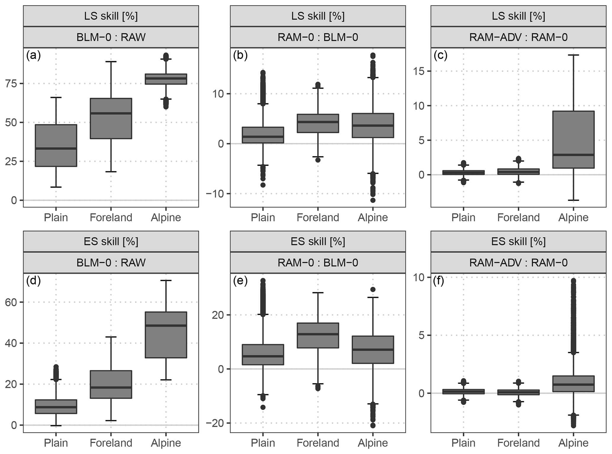
Figure 9 Aggregated skill scores (LS: a–c, ES: d–f) for groups of respective five weather stations which are located in the plain, in the mountain foreland near the Alps, or within an alpine valley. Each box-whisker contains boot-strapped mean values of the forecast steps from +12 to +72 h at a 12-hourly temporal resolution for all included stations. The scores are based on the full predictive bivariate distribution for the out-of-sample validation period. Compared are the BLM-0 model with the raw EPS as a reference, setup RAM-0 with setup BLM-0 as a reference, and the RAM-ADV correlation specification with the RAM-0 correlation model as a reference. Skill scores are in percent; positive values indicate improvements over the reference.

The post-processing employed by the simplest model, BLM-0, already shows a distinct improvement over the raw EPS with the largest values for alpine valley sites. In terms of the ES, the skill scores range between mean values of 10 % for the plain sites and 45 % for the alpine valley sites (Fig. 9d). A similar picture with an overall larger magnitude is shown for LS (Fig. 9a). In the comparison of the two different setups for the location or scale part (Fig. 9b, e), the more flexible setup is better regarding both scores for all station types; the largest improvements are found for stations located in the foreland, followed by stations within alpine valleys. The validation of the correlation models (Fig. 9c, f) shows that the flexible estimation of the correlation dependence structure is clearly superior only for station sites within an alpine valley.

5 Discussion and conclusion

In this study, we model the zonal and meridional wind components employing the bivariate Gaussian distribution in a distributional regression framework. In contrast to previous studies all distribution parameters, namely the location and scale parameters for both wind components but also the correlation coefficient between them, are estimated simultaneously. The overall performance of the models is evaluated for three groups of station types classified as topographically plain, mountain foreland, and alpine valley sites.

Section 5.1 discusses the benefits of the rotation-allowing model setup, RAM-0, over the baseline model, BLM-0. In Sect. 5.2, the different correlation models are discussed regarding the potential reason why the improvement of the predictive performance obtained with the more flexible correlation model is relatively small. At the end, in Sect. 5.3, a recommendation is given for which statistical model should be used in matters of simplicity and performance.

5.1 Rotation-allowing model setup

The rotation-allowing model (RAM-0) utilizes the zonal and meridional ensemble wind forecasts for both components of the two-dimensional location and scale parameters. This allows the statistical model to adjust for potential misspecifications in the ensemble wind direction by a smooth rotation conditional on the day of the year and the forecasted wind direction. For stations in complex terrain, this may be particularly advantageous due to unresolved topographical features.

The estimated effects confirm a distinct wind rotation for the valley site (Innsbruck), while for the station in the plain (Hamburg) barely any adjustments of the forecasted wind direction are needed (see Fig. 4). In terms of predictive performance, the more flexible model, RAM-0, outperforms the baseline model, BLM-0, for almost all times and stations (see Fig. 9b, e). However, the increase in predictive skill is similar for all three station types. This indicates that – even if no or only little rotation is needed – additional covariates usually yield a better adjustment of the distribution parameters and therefore an increased predictive skill. Furthermore, the results indicate that EPS wind forecasts in complex terrain are not solely tilted due to unresolved valley topographies, but show little skill on average. Thus, for alpine valley sites the rotation-allowing model mainly captures climatological properties conditional on the forecasted EPS wind direction. In accordance with this analysis, larger improvements can be found for stations located in the mountain foreland where the EPS has a higher information content and a certain rotation might be necessary.

These findings are supported by an additional comparison against the model inspired by Pinson (2012), which only uses a linear transformation of both wind components for the location parameters. The results show that a more flexible rotation-allowing specification is required to capture strong wind distortions; the full comparison is shown in Appendix C2.

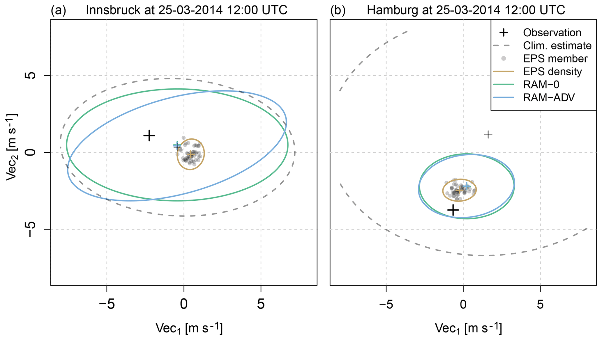
Figure 10 Two exemplary forecasts showing the respective observation (black cross), the climatological estimate (gray dashed line), the EPS member forecasts (gray points) and their empirical density (brown line), and the estimated bivariate distributions for the setups RAM-0 and RAM-ADV, without (green line) and with (blue line) modeled correlation, respectively. The climatological estimate uses the mean, the standard deviation, and the correlation of the observed wind components as bivariate distribution parameters. The lines show the 95 % percentiles of the respective bivariate distribution, the small crosses the ellipsoid centers or the location parameters. The shown observations and forecasts are valid at Innsbruck (a) and Hamburg (b) for 25 March 2014 12:00 UTC (forecast step +12 h). The forecasts are characteristic for (a) a valley station and (b) a station in the plain within our study.

5.2 Correlation specifications

Several different model specifications for the correlation parameter have been tested, among others a flexible setup employing wind direction and speed as potential covariates for the correlation parameter by nonlinear smooth effects following the idea of Schuhen et al. (2012). The estimated correlation parameters seem to be reasonable, and show, on average, larger values for Innsbruck than for Hamburg (see Fig. 6 for forecast step +12 h). In terms of predictive skill, all models tested show only minor improvements compared to the models with zero correlation. The improvements are highest for stations located inside alpine valleys, with a mean improvement of 1 % in terms of ES and 5 % in terms of LS skill scores (see Fig. 9c, f). The relatively small benefits due to the explicit estimation of the correlation are confirmed by the results of an additionally tested model based on Schuhen et al. (2012) (Appendix C1).

As an illustration of the potential reasons for no more pronounced enhancements by an explicit estimation of the dependence structure, Fig. 10 shows exemplary forecasts for a station located within an alpine valley (Innsbruck; Fig. 10a) and in the plains (Hamburg; Fig. 10b). The figure shows the raw EPS members (gray points) plus the respective observations (black crosses), climatological estimates (gray dashed lines), and the corresponding post-processed bivariate distributions without (green lines) and with (blue lines) an explicitly estimated correlation parameter. For the valley station, the raw EPS has only little skill and the uncertainty of the post-processed bivariate distributions tends towards the climatological estimate. Although a distinct correlation is estimated by the RAM-ADV model, the variance is still in the same range as for the RAM-0 model. In contrast, for the station in the plain the uncertainty of the post-processed predictions is much smaller than the uncertainty of the climatological estimate due to a higher information content of the EPS. The estimated correlation is close to zero and the predictions of RAM-0 and RAM-ADV look almost identical with a similar elliptic shape as the raw EPS. This means that for locations where the ensemble provides only little information, the post-processed uncertainty is rather large and the statistical model tries to capture unexplained features by the correlation parameter. For stations where the predictive skill of the raw ensemble is already high, the statistical models get valuable information about the expected wind situation and are able to accurately specify the location and scale parameters. Thus, the correlation of the residuals becomes less important and typically smaller. This interpretation is supported by the probabilistic scores used in this study which show improvements in the RAM-ADV models mainly for alpine valley sites where the skill of the raw ensemble is rather low.

5.3 Proposed model specification

The study shows that the flexible rotation-allowing models bring significant performance benefits for stations located in complex terrain as well as for stations in the plain. Therefore, we propose using a similar setup employing both EPS wind components by a smooth rotation-allowing framework. For correlation, we have not found a clear distinction between the different correlation models tested for stations located in the plain and the foreland. For stations located within an alpine valley, minor improvements could be found. Despite these somewhat unexpected findings, this has clear advantages for operational usage: estimating a single bivariate response distribution forcing the correlation dependence structure to zero is the same as post-processing each wind component separately in a univariate setup with marginal Gaussian response distributions. A univariate post-processing approach for each respective wind component simplifies the estimation process in terms of complexity of the required statistical models and reduces computational time with only little loss of predictive skill, at least for the stations tested in this study.

Appendix A: Model specification complements

A1 Smooth functions

Generalized additive models (GAMs, Hastie and Tibshirani, 1986) and generalized additive models for location, shape, and scale (GAMLSS, Rigby and Stasinopoulos, 2005) are generalizations of linear regression models which allow one to include potentially nonlinear (and even multi-dimensional) effects in the linear predictors η. Nonlinear terms are frequently approximated by smooth functions, also referred to as regression splines. These regression splines are directly linked to the model parameters as additive terms in η and allow the statistical model to include nonlinear transformations of a specific covariate, if needed. For further details a comprehensive introduction to GAMs is given in Wood (2017). An example of an additive predictor η with a smooth function is

$$\begin{array}{}\text{(A1)}& \mathit{\eta }={\mathit{\alpha }}_{\mathrm{0}}+\underset{\text{linear effect for }{x}_{\mathrm{1}}}{\underbrace{f_{\mathrm{1}}\left(x_{\mathrm{2}}\right){\mathit{\alpha }}_{\mathrm{1}}\cdot x_{\mathrm{1}}}}+\underset{\text{pot. nonlinear effect for }{x}_{\mathrm{2}}}{\underbrace{f_{\mathrm{1}}\left(x_{\mathrm{2}}\right)}},\end{array}$$

where α_• are regression coefficients, x_• the covariates, and α₁⋅x₁ and f₁(x₂) a linear and a potentially nonlinear one-dimensional effect, respectively. Generally, f₁ can be any transformation of the covariate x₂ dependent on the specification of f₁. For periodic values smooth “cyclic” splines are often applied, meaning that the function has the same value at its upper and lower boundaries. This is similar to applying a linear combination of (several) trigonometric functions, as, e.g., performed by Schuhen et al. (2012). In this study, we utilize “cubic” smooth functions with cyclic constraints. A detailed description of cyclic cubic regression splines is given in Wood (2017, chap. 4.1.3).

A2 Time-adaptive training scheme

To account for seasonal variations of the intercept and the linear coefficients, seasonal cyclic splines are used. If the covariates provide sufficient information, a time-adaptive training scheme might not be required. However, if the bias and/or the slope coefficient are not constant throughout the year or the covariate's skill varies over the year, these terms are mandatory to allow the statistical model to depict seasonal features.

We therefore fit one statistical model over a training data set including several years of data, but allow the coefficient included in the linear predictor(s) η to smoothly evolve over the year:

$$\begin{array}{}\text{(A2)}& \begin{array}{rl}\mathit{\eta }& =\underset{\begin{array}{c}\text{seasonally varying}\\ \text{intercept}\end{array}}{\underbrace{{\mathit{\alpha }}_{\mathrm{0}}+{f_{\star }}_{\mathrm{0}}\left(\mathrm{doy}\right)}}+\underset{\begin{array}{c}\text{seasonally varying}\\ \text{coefficient for }{x}_{\mathrm{1}}\end{array}}{\underbrace{({\mathit{\alpha }}_{\mathrm{1}}+f_{\mathrm{1}}(\mathrm{doy}\left)\right)}}\cdot x_{\mathrm{1}}+\mathrm{\cdots }\\ & +\underset{\begin{array}{c}\text{seasonally varying}\\ \text{coefficient for }{x}_n\end{array}}{\underbrace{({\mathit{\alpha }}_n+f_n(\mathrm{doy}\left)\right)}}\cdot x_n.\end{array}\end{array}$$

As before, α_• are the regression coefficients, x_• are the covariates, and f_•(doy) employ cyclic regression splines conditional on the day of the year (doy). Within this study, we refer to the regression coefficients α_• also as global intercept or slope coefficients to emphasize that they are unconditional on the day of the year.

Appendix B: Skill scores used for verification

To compare the different bivariate Gaussian models of this study, we employ skill scores. A skill score shows the improvements over a reference. For all measures with a perfect score of zero, the skill score simplifies to

$$\begin{array}{}\text{(B1)}& \mathrm{skill}\mathrm{score}={\displaystyle \frac{{\mathrm{score}}_{\mathrm{fcst}}-{\mathrm{score}}_{\mathrm{ref}}}{{\mathrm{score}}_{\mathrm{opt}}-{\mathrm{score}}_{\mathrm{ref}}}}=\mathrm{1}-{\displaystyle \frac{{\mathrm{score}}_{\mathrm{fcst}}}{{\mathrm{score}}_{\mathrm{ref}}}},\end{array}$$

where score_fcst is the forecast's score, score_opt=0 refers to a hypothetical optimal or perfect score, and score_ref is the score for the reference (Gneiting and Raftery, 2007).

In this study we use the logarithmic score (LS, Good, 1952) and the energy score (ES, Gneiting and Raftery, 2007) to validate the probabilistic performance of the bivariate Gaussian predictions of the statistical post-processing models. Both multivariate scores evaluate the full predictive distribution returned by the statistical models.

The calculation of the ES is based on the R package scoringRules (Jordan et al., 2019). For a predictive distribution f on ℝ^d given through m discrete samples ${\mathit{X}}_{\mathrm{1}},\mathrm{\dots },{\mathit{X}}_m$ from f with ${\mathit{X}}_i=(X_i^{\left(\mathrm{1}\right)},\mathrm{\dots },X_i^{\left(d\right)})\in {\mathbb{R}}^d,i=\mathrm{1},\mathrm{\dots },m$, the ES can be written as

$$\begin{array}{}\text{(B2)}& \mathrm{ES}(f,\mathit{y})={\displaystyle \frac{\mathrm{1}}{m}}\sum _{i=\mathrm{1}}^m\Vert {\mathit{X}}_i-\mathit{y}\Vert -{\displaystyle \frac{\mathrm{1}}{\mathrm{2}{m}^{\mathrm{2}}}}\sum _{i=\mathrm{1}}^m\sum _{j=\mathrm{1}}^m\Vert {\mathit{X}}_i-{\mathit{X}}_j\Vert ,\end{array}$$

where $\Vert \cdot \Vert$ denotes the Euclidean norm on ℝ^d and $\mathit{y}=(y^{\left(\mathrm{1}\right)},\mathrm{\dots },y^{\left(d\right)})\in {\mathbb{R}}^d$ the multivariate observation. The calculation of the ES for all post-processed forecasts is based on m=1000 random draws from the bivariate Gaussian distribution.

The logarithmic score is defined based on the log-density (or log-likelihood):

$$\begin{array}{}\text{(B3)}& \mathrm{LS}(f,\mathit{y})=\log \left(f\right(\mathit{y}\left)\right),\end{array}$$

where the probabilistic forecast on ℝ^d is given by the probability density function f, and $\mathit{y}=(y^{\left(\mathrm{1}\right)},\mathrm{\dots },y^{\left(d\right)})\in {\mathbb{R}}^d$ is the multivariate observation (Jordan et al., 2019). However, it is not possible to compute skill scores based on the LS from Eq. (B3). The reason is that the LS for a perfect prediction is not zero but actually diverges to infinity. To mitigate this shortcoming we follow Lindsey (1996, chap. 3.2.1) and define the likelihood based on the cumulative distribution function F on an interval of length Δ rather than the density at a single point:

$$\begin{array}{}\text{(B4)}& f\left(\mathit{y}\right)\approx {\displaystyle \frac{F(\mathit{y}+\mathbf{\Delta }/\mathrm{2})-F(\mathit{y}-\mathbf{\Delta }/\mathrm{2})}{\mathbf{\Delta }}},\end{array}$$

where Δ is set to the precision of reporting y. Employing this idea, the LS can be approximated (up to a constant) by

$$\begin{array}{}\text{(B5)}& \mathrm{LS}(f,\mathit{y})\propto \log \left(F\right(\mathit{y}+\mathbf{\Delta }/\mathrm{2})-F(\mathit{y}-\mathbf{\Delta }/\mathrm{2}\left)\right).\end{array}$$

This representation has the advantage that for a perfect fit the LS is zero as $F(\mathit{y}+\mathbf{\Delta }/\mathrm{2})=\mathrm{1}$ and $F(\mathit{y}-\mathbf{\Delta }/\mathrm{2})=\mathrm{0}$ so that $\mathrm{LS}=\log (\mathrm{1}-\mathrm{0})=\mathrm{0}$. Consequently, the corresponding skill scores can be computed as shown in Eq. (B1). In this study, we use $\mathbf{\Delta }/\mathrm{2}=\mathrm{0.1}$ m s⁻¹; the computation of the bivariate cumulative distribution function is based on the R package mvtnorm (Genz and Bretz, 2009). For the discrete raw ensemble forecasts of wind vectors, the empirical mean and covariance matrix of the ensemble are used to calculate the LS as in Eq. (B5). This implicitly assumes that the raw ensemble wind forecasts follow a bivariate Gaussian distribution.

Appendix C: Further model comparisons

To benchmark the models as presented in this study, we compare our specifications to those of Schuhen et al. (2012) and Pinson (2012).

C1 Comparison with Schuhen et al. (2012)

Schuhen et al. (2012) fit a bivariate Gaussian model for the wind components in three phases. First, they fit the correlation parameter as a trigonometric function of the ensemble mean wind direction by weighted nonlinear least squares. They estimate the regression coefficients for the correlation parameter offline in a pre-processing step for a separate year, either for a single site or a group of stations. The adjustment for a suitable number of trigonometric cycles must be done manually, which can be prone to errors according to Schuhen et al. (2012, p. 3207). Second, univariate models are fitted for the components of the two-dimensional location parameter by standard linear regression. Third, the two-dimensional variance parameter of the bivariate Gaussian distribution is estimated by maximum likelihood keeping all other parameters fixed. In contrast to the first phase, the estimation within the second and third phases is performed online using a rolling training period, either for a single site or a group of stations.

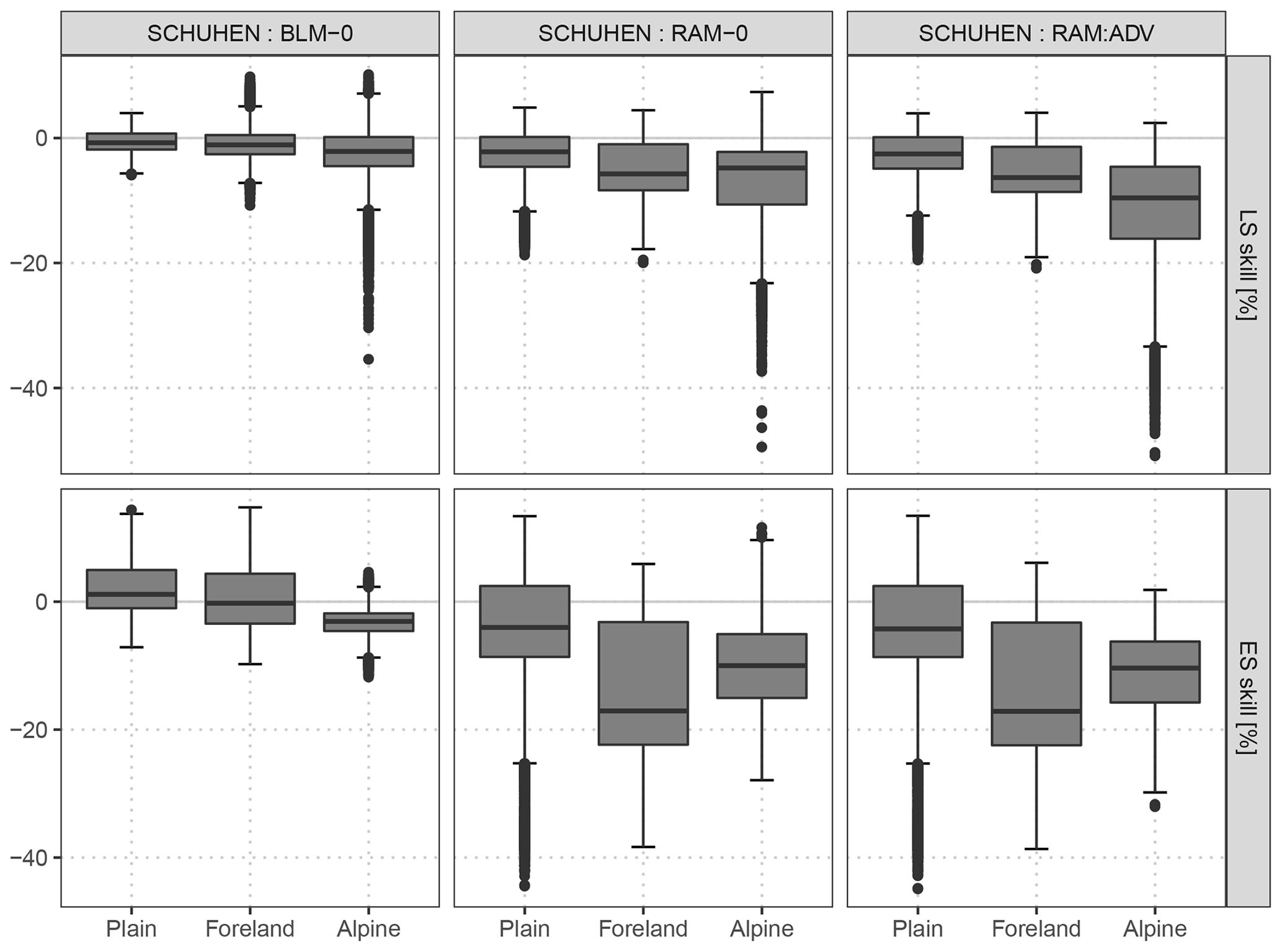
Figure C1 As Fig. 9, but an adaption of the Schuhen et al. (2012) model is compared to the baseline model BLM-0, to the rotation-allowing model without correlation RAM-0, and to the rotation-allowing model with correlation RAM-ADV.

In this study, we apply Schuhen et al. (2012) using the implementation of Lerch (2019). As the focus of the current paper is on post-processing wind vector forecasts for stations with different site characteristics, we perform the estimation for each station separately. We use a rolling training period of 40 days and employ two periods for the trigonometric function in the estimation of the correlation parameter on the training data set. Figure C1 shows the comparison to the baseline model BLM-0, to the rotation-allowing model without correlation RAM-0, and to the rotation-allowing model with correlation RAM-ADV for the out-of-sample validation period of this study. The predictive performance of Schuhen et al. (2012) is overall comparable to the BLM-0 setup. Accordingly, the comparison to RAM-0 and RAM-ADV confirms that within this study the largest potential for improvement lies in the correct specification of the location and scale parameters of the bivariate Gaussian distribution.

C2 Comparison with the Pinson (2012)-type model

Since one of the major aspects within this study is the rotation of the wind direction, we compare our models to a model inspired by Pinson (2012), which also uses both wind components of the raw ensemble as predictors for both components of the bivariate location parameter. We define the two-dimensional location and scale part according to Pinson (2012), but employ our model framework and fix the correlation to zero, i.e., by

$$\begin{array}{}\text{(C1)}& \begin{array}{rl}& {\mathit{\mu }}_{\star }={{\mathit{\alpha }}_{\star }}_{\mathrm{0}}+{f_{\star }}_{\mathrm{0}}\left(\mathrm{doy}\right)+({{\mathit{\alpha }}_{\star }}_{\mathrm{1}}+{f_{\star }}_{\mathrm{1}}(\mathrm{doy}\left)\right)\cdot {\mathrm{vec}}_{\mathrm{1},\mathrm{mean}}\\ & +({{\mathit{\alpha }}_{\star }}_{\mathrm{2}}+{f_{\star }}_{\mathrm{2}}(\mathrm{doy}\left)\right)\cdot {\mathrm{vec}}_{\mathrm{2},\mathrm{mean}},\\ & \log \left({\mathit{\sigma }}_{\star }\right)={{\mathit{\beta }}_{\star }}_{\mathrm{0}}+{g_{\star }}_{\mathrm{0}}\left(\mathrm{doy}\right)+({{\mathit{\beta }}_{\star }}_{\mathrm{1}}+{g_{\star }}_{\mathrm{1}}(\mathrm{doy}\left)\right)\\ & \cdot {\mathrm{vec}}_{\star ,\log .\mathrm{sd}},\\ & \mathrm{rhogit}\left(\mathit{\rho }\right)=\mathrm{0},\end{array}\end{array}$$

where, as before, α_• and β_• are regression coefficients and f_• and g_• are cyclic regression splines. The location part employs a linear transformation of the wind components, which is able to rotate the wind direction but in a restricted linear manner.

Figure C2 As Fig. 9, but the model specification inspired by Pinson (2012) (Eq. C1) is compared to the baseline model BLM-0, to the rotation-allowing model without correlation RAM-0, and to the rotation-allowing model with correlation RAM-ADV.

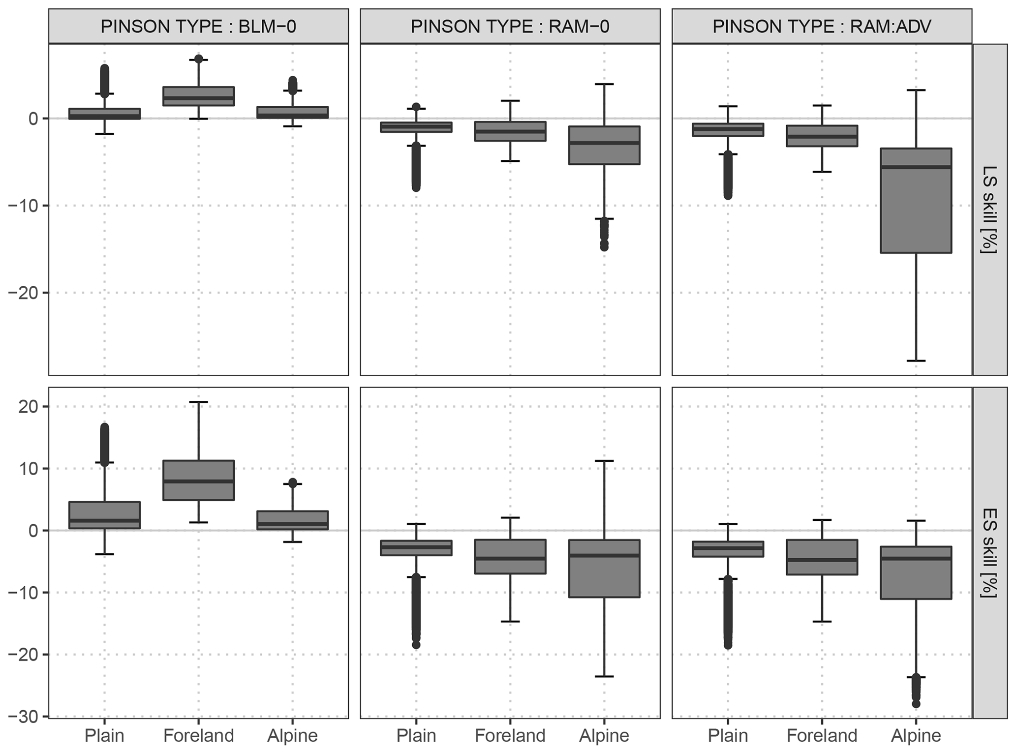
Figure C2 shows the comparison of the Pinson-type model to this study's baseline model BLM-0, to the rotation-allowing model without correlation RAM-0, and to the rotation-allowing model with correlation RAM-ADV for the out-of-sample validation period. The results show that the Pinson-type model is apparently a mixture of the BLM-0 and RAM-0 models. Hence, for minor distortions in wind directions, such as in the foreland, the Pinson-type model is already sufficient and has clear benefits when compared to the non-rotation-allowing BLM-0 model. For stations in complex terrain, the RAM-0 model shows clear advantages over the less flexible Pinson-type model. This indicates that a more flexible rotation-allowing specification is required to capture strong wind distortions, e.g., due to discrepancies between the model and real topography. The explicit estimation of the correlation (RAM-ADV) further increases the performance, but mainly for alpine stations (see Sect. 5.2).