the Creative Commons Attribution 4.0 License.
the Creative Commons Attribution 4.0 License.
 | 21 Nov 2019
Automated detection of weather fronts using a deep learning neural network
Kenneth E. Kunkel
Deep learning (DL) methods were used to develop an algorithm to automatically detect weather fronts in fields of atmospheric surface variables. An algorithm (DL-FRONT) for the automatic detection of fronts was developed by training a two-dimensional convolutional neural network (2-D CNN) with 5 years (2003–2007) of manually analyzed fronts and surface fields of five atmospheric variables: temperature, specific humidity, mean sea level pressure, and the two components of the wind vector. An analysis of the period 2008–2015 indicates that DL-FRONT detects nearly 90 % of the manually analyzed fronts over North America and adjacent coastal ocean areas. An analysis of fronts associated with extreme precipitation events shows that the detection rate may be substantially higher for important weather-producing fronts. Since DL-FRONT was trained on a North American dataset, its extensibility to other parts of the globe has not been tested, but the basic frontal structure of extratropical cyclones has been applied to global daily weather maps for decades. On that basis, we expect that DL-FRONT will detect most fronts, and certainly most fronts with significant weather. However, where complex terrain plays a role in frontal orientation or other characteristics, it might be less successful.
- Article
(8965 KB) - Full-text XML
- BibTeX
- EndNote


Fronts are defined as the interface or transition zone between two air masses of different density (American Meteorological Society, 2018). Almost invariably, these air masses are characterized by contrasting temperature, pressure, moisture, and wind fields. The canonical structure of an extratropical cyclone (ETC) is distinguished by fronts demarcating the different air masses that provide the potential energy for such systems.
Fronts are centrally important because they are usually formed by lower tropospheric horizontal convergence and associated upward vertical motion arising from large-scale dynamical pressure forces in the atmosphere. The upward vertical motion is associated with a variety of significant weather events, including severe thunderstorms and a wide spectrum of precipitation types and amounts. Thus, front locations are also areas of enhanced probability of significant weather. Kunkel et al. (2012) found that in the US more than half of extreme precipitation events exceeding the threshold for a 1-in-5-year average recurrence interval occurred in the vicinity of fronts.
Manual front identification by weather map analysis is a labor-intensive process. This provides a strong motivation for developing accurate automated approaches for operational applications. When considering the analysis of climate model simulations, such as the Coupled Model Intercomparison Project Phase 5 (CMIP5) and upcoming Phase 6 (CMIP6) suites, manual analysis is not feasible because of the large number of simulated days (requiring analysis of hundreds of thousands of individual days or hours). Automated approaches are essential. The immediate motivation for this work was the need to evaluate frontal occurrences in CMIP5 climate model simulations with a specific interest in extreme precipitation events related to fronts.
Fronts are elongated in one dimension. Thus, the simple representation of a front often used by meteorologists is a curved line. As such, the development of automated methods differs from those of certain other important phenomena such as ETC centers and tropical cyclones, where a point minimum in pressure is a suitable simplification of location. Several automated methods have been developed to identify fronts with varying degrees of success. In this paper we describe a novel approach using a deep learning neural network (DLNN). Section 2 is a discussion of previously published automated algorithms. Section 3 is a description of our algorithm. Section 4 is a presentation of the training results and the results of comparing fronts detected using the algorithm with fronts that were manually identified by National Weather Service (NWS) meteorologists as part of their operational forecasting activities. Section 5 describes climatological information derived from the application of the algorithm. In Sect. 6 we discuss the effective use of the algorithm.
Previous efforts to develop automated front detection algorithms have generally calculated horizontal fields of the Laplacian of a surface parameter. Fronts are associated with high values of the Laplacian, i.e., areas where the parameter gradient is changing rapidly in space. In most cases, the parameter includes a thermal element, but not always. Hewson (1998) used the wet bulb potential temperature, θw, which incorporates atmospheric water vapor content along with temperature. Berry et al. (2011) and Catto et al. (2012) also used θw. Jenkner et al. (2010) and Schemm et al. (2015) used equivalent potential temperature, θe, which incorporates atmospheric water vapor differently. It is not clear on first principles whether there would be substantial differences between θw and θe in frontal detection. Since atmospheric water vapor content is usually directly correlated with temperature (e.g., higher absolute moisture associated with higher temperature) in the vast majority of atmospheric conditions at the surface, the use of potential temperature metrics that incorporate moisture will lead to higher numeric differences between cold and warm air masses. By contrast, Simmonds et al. (2012), Schemm et al. (2015), and Huang et al. (2017) examined the use of surface wind as the sole variable. They found this approach to be successful, although such an approach would be more vulnerable to labeling areas with no density gradients as fronts. Parfitt et al. (2017) defined a parameter as the product of the relative vorticity (ζ) and potential temperature (θ). In this case, the identification of a front is more stringent, requiring both a wind shift and a temperature change.
In each of these previous studies, it was necessary to choose a single parameter, which can be a combination of individual state variables, on which to perform the analysis. The parameter can be chosen/constructed to best reflect a physical understanding of the characteristics of fronts, but there is no obvious flexible way to incorporate other atmospheric fields to improve performance. Wong et al. (2008) used a genetic algorithm to identify a set of weather system types; this approach in principal can incorporate a large set of fields, although as they applied it, a limited choice of variables is still necessary to identify a feature as a particular type of meteorological system. Also, the performance of an algorithm was typically evaluated based on qualitative comparisons of the objectively identified fronts with manually drawn fronts, usually for a small number of situations. Quantitative performance metrics were not provided in any of these studies.
It should be noted that Sanders and Hoffman (2002) draw a distinction between the fronts that are analyzed on surface weather maps and baroclinic zones, showing that the former are often not characterized by a density difference. Sanders (2005) argues that it is not acceptable to label such areas as fronts since density differences are required to produce key dynamical characteristics of ETCs. However, the drawing of fronts where there are wind shifts and/or pressure troughs, but no temperature difference, remains common practice among national meteorological services because of the accompanying weather changes, e.g., winds, sky conditions.
3.1 Deep learning neural network (DLNN)
In operational meteorological analysis, fronts are identified visually based on the approximate spatial coincidence of a number of quasi-linear localized features: a trough (relative minimum) in air pressure in combination with gradients in air temperature and/or humidity and a shift in wind direction (Stull, 2015). Fronts are categorized as cold, warm, stationary, or occluded, with each type exhibiting somewhat different characteristics. The DLNN described herein is designed to mimic the visual fronts recognition task performed by meteorologists.
The goal for the DLNN front detection algorithm (DL-FRONT) differs from that in many visual recognition problems. Front detection does not involve identification of whole-image characteristics or distinct, bounded regions. Instead, the goal is to estimate the likelihood that each cell in a geospatial data grid lies within a frontal zone of a particular category – cold, warm, stationary, occluded, or none. The “none” category allows the algorithm to positively identify cells that do not appear to lie within any front region. These results are then used to identify paths along which there is a maximum likelihood that a front of a particular type is present in order to produce front lines similar to those drawn by meteorologists.
As explained by Goodfellow et al. (2016), “deep learning” (DL) refers to machine learning algorithms that use multiple layers of non-linear transformations to derive features from input fields. Each successive layer learns to transform the output from one or more previous layers into ever more abstract, conceptual representations of the original inputs. The outputs of a layer are called feature maps in recognition of their conceptual character. Most of these DL algorithms are composed of artificial neural networks (NNs), with 2-D convolutional neural networks (CNNs) in common use for learning to detect features in image arrays. Our network uses a technique known as supervised learning, where a “labeled” dataset containing the desired network outputs for each input is compared with the network outputs, and the differences between them are used to modify the non-linear transformations in the different layers (Deng and Yu, 2014).
Our DL-FRONT network is built using five different types of layers, which are described below. They are: 2-D convolution layers, rectified linear unit (ReLU) layers, 2-D dropout layers, 2-D zero-padding layers, and a softmax layer. A network layer operates on a data grid composed of a set of 2-D spatial arrays (dimensions indicated by the indices i and j in the equations that follow), where each spatial array in the set contains values for a different measurement type or feature (indicated by the indices k and/or l). This third dimension is the “feature” dimension in the discussion below.
The 2-D convolution layer is a core component of most 2-D CNNs. Spatial filters are convolved with an input data grid to produce an output data grid as shown in Eq. (1).
The kth feature map of the output data grid, Ok, is produced by summing the convolutions of a set of filter kernels, fkl, with the feature maps, Il, of the input data grid and adding a bias, bk, to each cell of the result. Each filter kernel, fkl, is an M×N grid of convolution weights. The number of input feature maps, L, is not usually mentioned when describing 2-D convolution layers, so a layer is described as having an M×N kernel and K filters.
The ReLU layer and the softmax layer are examples of activation layers. An activation layer produces an output by applying a nonlinear function to an input, and it is critical to the function of any NN. A NN without nonlinear activation layers would be limited to producing linear superpositions of its inputs. The introduction of nonlinearity makes it possible for a NN to approximate any continuous real function of multiple variables (Kolmogorov, 1957) (Cybenko, 1989). Neilsen (2015) describes how activation functions allow the different elements, or neurons, within a NN to interact with one another to produce arbitrary functions of the inputs.
The ReLU layer function in Eq. (2) is piecewise continuous. It produces nonlinearity by setting the output to zero when the input value is negative and setting the output value to the input value when the input value is positive. The ReLU layer applies this function element-wise to the input data grid.
The softmax layer function in Eq. (3), unlike the ReLU layer function, is applied to each feature vector in an input data grid, I, producing an output data grid, O, of the same dimensions.
The softmax function transforms the elements of a feature vector from activation intensities into probability estimates for each feature. It scales the elements of each feature vector to a range of zero to one, increases the dynamic range between the largest and smallest values, and makes the elements sum to a value of 1. The softmax layer is typically used as the last layer in a network when the desired output is category labels instead of continuous function values.
The 2-D dropout layer is used to help prevent overfitting (Hinton et al., 2012). An overfit network will show high accuracy on the training set, but it will perform poorly on data it has not seen during training. The 2-D dropout layer function transforms an input data grid into an output data grid by setting a fraction of the feature maps to zero. The feature maps to set to zero are chosen at random in each training iteration. The feature maps that have been set to zero make no contribution to the next layer, which forces the network as a whole to find a more general solution that is robust to missing information. Dropout layers make it more difficult for the network to encode an exact response to each training input and are only functional during network training. No feature maps are set to zero when the network is not being trained.
The zero-padding layer transfers an input data grid to an output data grid that has the same size in the feature dimension but is larger by some number of rows and columns of cells in the spatial dimensions. The unfilled cells in the output data grid contain values of zero. The input data grid is usually centered within the output data grid. A zero-padding layer is often used to counteract the spatial shrinking effect produced by a 2-D convolution layer, which produces an output data grid that is M−1 rows and N−1 columns smaller than its input, where M and N are the spatial dimensions of the 2-D convolution filter. The zero-valued elements make no contribution to the next layer.
The DL-FRONT 2-D CNN is trained by iteratively optimizing the values of the weights and biases in the convolution filters to minimize the difference between a labeled dataset and a “predicted” dataset produced by the network from a corresponding input dataset. The difference is measured using a cost, or loss, function. We use the categorical cross-entropy loss function (Eq. 4) for training the network, which has the form
where H(pt) is the magnitude of the loss, p is a set of category vectors taken from the network output, t is a corresponding set of category vectors from the labeled dataset, w is a per-category weight, I is the number of vectors, and C is the number of categories. Each predicted and label vector has five elements, one for each of the five possible cold, warm, stationary, occluded, and none categories. Each label vector is assigned one and only one category by giving the appropriate element a value of 1 and the others a value of 0. The elements of each predicted vector contain values between 0 and 1, inclusive, which are the estimated category likelihoods for that cell. The lower the likelihood value in the predicted vector for the category marked as correct in the label vector, the larger the contribution to the loss. The per-category weights are used to adjust the relative significance of the contributions from the different categories. Approximately 88 % of our data grid cells have no front present, so the loss function is at risk of being dominated by the contribution of the none category. Reducing the weight for the none category relative to the weights for the other categories will make the loss function less sensitive to that category. Similarly, increasing the weight for a seldom-seen category will make the loss function more sensitive to that category.
The Adam adaptive moment estimation technique (Kingma and Ba, 2015) is the loss minimization strategy used when training the network. Adam is a form of stochastic gradient descent (SGD) that has been shown to perform well in a variety of networks. As with most SGD techniques, Adam has a primary initial learning rate parameter. The learning rate sets the initial magnitude range of the changes to the network weights and biases.
We implemented the DL-FRONT network in Python using numpy (van der Walt et al., 2011) and the Keras deep learning library (Chollet, 2015) on both Tensorflow (Abadi et al., 2015) and The Theano Development Team et al. (2016) (Bergstra, 2010) computational backends. The training application made use of the scikit-learn package (Pedregosa et al., 2011) to provide k-fold cross-validation and hyperparameter search. The “outer” network parameters such as learning rate, number of layers, etc. are referred to as hyperparameters. A significant part of the time spent developing a NN is devoted to optimizing the hyperparameters.
We initially chose a network based on 2-D convolution layers with 5×5 kernels because of the structural similarity we saw between a layer of this sort and a finite-difference second-order spatial derivative function. The visual front detection task described at the beginning of this section, if expressed mathematically, can be thought of as synthesizing the results of various spatial derivatives of the different input measurements at each point in the data grid.
We experimented with the basic architecture with a series of hyperparameter searches using training runs of 100–200 epochs over a 1-year batch of data. An epoch is one full pass through the training data. The experiments used the scikit-learn GridSearchCV function to perform multiple training runs, each with a different combination of learning rate, category weights, number of 2-D convolution layers, sizes of layer kernels, and numbers of filters in layer kernels. The hyperparameter combination from these experiments that produced the best validation accuracy and loss was chosen for training for 1200 epochs over 5 years of data. The details of these experiments are outside the scope of this paper. The amount of time required to do an exhaustive search of all hyperparameter combinations and ranges makes such a task impractical. The highest accuracy and lowest loss in training and validation out of the experiments we performed was with the network described below.
Figure 1 shows a schematic of the resulting DL-FRONT 2-D CNN architecture. At the far left of the figure is the input data grid, which is composed of five “feature maps” of 2-D meteorological fields (as compared to three feature maps of 2-D color fields for an RGB image) on a 1∘ geospatial grid. These meteorological fields are 3-hourly instantaneous values of air temperature at 2 m, specific humidity at 2 m, air pressure reduced to mean sea level, the east–west (u) component of wind velocity at 10 m, and the north–south (v) component of wind velocity at 10 m. The meteorological fields were obtained from the Modern-Era Retrospective Analysis for Research and Applications, Version 2 (MERRA-2; Gelaro et al., 2017) and were sampled on a 1∘ latitude–longitude grid over a domain of 10–77∘ N and 171–31∘ W. We obtained 37 984 sets of grids for the time span 2003–2015.
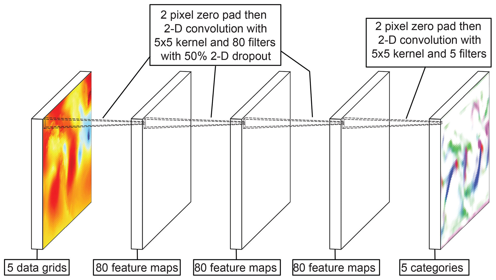
Figure 1Schematic of the DL-FRONT 2-D CNN architecture. The five category input data grid on the left contains the five input surface meteorological 2-D fields (temperature, humidity, pressure, u-component of wind, v-component of wind). The five-category output data grid on the right contains five 2-D likelihood estimates for the five front categories (cold, warm, stationary, occluded, and none).
The first network layer is a composite of a 2-D zero-padding layer, a 2-D convolution layer with a 5×5 kernel and 80 filters, a ReLU activation layer, and a 50 % 2-D dropout layer. The output of this layer is a data grid that has the same spatial extent and 80 abstract feature maps. The next two layers have the same basic structure, producing output data grids with 80 feature maps that have the same spatial extent as the original input data grid.
The fourth network layer is different from the other three. This layer is a composite of a 2-D zero-padding layer, a 2-D convolution layer with a 5×5 kernel and 5 filters, and a softmax activation layer. The output is a data grid with 5 categories (cold, warm, stationary, occluded, and none) that has the same spatial extent as the original input data grid.
We found through our experiments that, compared to no weighting, setting the category weight for the none category to 0.35 and the other weights to 1.0 improved the network accuracy for the other four categories without reducing the performance for the none category. Inverse weighting based on category frequency produced results that were worse than that for no weighting. We also found that learning rates in the range of 0.00005 to 0.0005 produced nearly identical network loss and accuracy. The final learning rate chosen was 0.0001.
3.2 Front polyline extraction
The output of the DL-FRONT 2-D CNN is a set of spatial grids that are, in essence, maps of likelihood of the presence of the five different front categories (cold, warm, stationary, occluded, and none). In order to use these results in follow-on studies, we needed to obtain polylines describing the locations of the front boundaries. We developed an application using numpy (van der Walt et al., 2011) and scikit-image (van der Walt et al., 2014) that traces out “ridgelines” of the likelihood fields for the different front types and reduces them to a set of latitude–longitude polylines labeled by front type.
The extraction of front polylines from a front likelihood data grid was initiated by creating a “one-hot” version of the data grid and an “any front” likelihood data grid. The one-hot data grid is of the same dimensions as the front likelihood data grid where each category vector in the data grid is altered to set the largest likelihood value to 1 and the other likelihood values to 0. This assigns a single front type (or “no front”) to each cell of the data grid. The 2-D “any front” likelihood data grid has the same spatial dimensions as the front likelihood data grid. The value for a cell in the “any front” data grid is the maximum likelihood value from the cold, warm, stationary, and occluded front elements of the corresponding category vector. Cells where the maximum likelihood in the corresponding category vector is for “no front” are set to 0. The “any front” likelihood data grid describes networks of fronts which are often connected and is used in the steps that follow because it helps ensure continuity in cases where the front category may change along a continuous boundary. For example, it is not uncommon for a front boundary to oscillate between cold and stationary.
Next, the divergence of the “any front” data grid at each cell in the grid is calculated using multiple applications of the numpy gradient function. All values in the divergence data grid greater than −0.005 are then set to zero, and a “mask” data grid is created that has a value of 1 wherever the modified divergence data grid is non-zero. The resulting divergence data grid has narrower features than the original data grid and tends to have sharp minima lines running down the centers of the front boundary regions.
The scikit-image medial_axis function from the morphology module is applied to produce a data grid of skeletonized front networks. The skeletonized front networks have the same structure as seen in the mask data grid, but they have been reduced to a width of one cell.
At this point, the one-hot data grid is used to segment the skeletonized front networks and divergence data grids, producing a pair of 3-D data grids with a category dimension. Each skeletonized front network cell and divergence value is now, in effect, labeled as belonging to a particular front type.
Each front type is processed in turn. For a given front type we use the scikit-image label function from the measure module to identify each separate contiguous piece of the skeletonized front network. For each piece just found we find the endpoints of the segment and then find the set of least-cost paths between those endpoints in the segmented divergence data grid using scikit-image minimum cost path (MCP) functions from the graph module. The result in each instance is a raster representation of a polyline. We then convert the raster to a polyline with the minimum number of vertices needed to reproduce the raster. Finally, the latitude and longitude values for the vertices are obtained to produce latitude–longitude polylines.
Once this process is completed for the front likelihood data grid for a single time step, we have a set of front boundary polylines for each front in that data grid. We write the polylines for each time step into a separate JSON file, identifying the time and organizing by front type. We now have a dataset similar to the original form of our labeled dataset, which is described in Sect. 3.3.
3.3 Labeled dataset
Our labeled dataset was extracted from an archive of NWS Coded Surface Bulletin (CSB) messages (National Weather Service, 2019). Each CSB message contains lists of latitudes and longitudes that specify the locations of pressure centers, fronts, and troughs identified by NWS meteorologists as part of the 3-hourly operational North American surface analysis they perform at the Weather Prediction Center (WPC). Each front or trough is represented by a polyline. We obtained a nearly complete archive of 37 709 CSBs for 2003–2015 from the WPC and produced a data grid for each time step by drawing the front lines into latitude–longitude grids that matched the resolution and spatial extents of the MERRA-2 input data grids with one grid per front category. Each front was drawn with a transverse extent of 3∘ (3 grid cells) to account for the fact that a front is not a zero-width line, and to add tolerances for possible transverse differences in position between the CSB polylines and front signatures in the MERRA-2 dataset. The training, validation, and evaluation described in the Results section were restricted to a region around North America (Fig. 2) where the rate of front crossings recorded by the CSBs was at least 40 per year in order to account for the focal nature of the WPC surface analyses.

Figure 2The mask applied to the data grids during training and evaluation. The area in dark red is the envelope of the areas where the CSB dataset shows that there are more than 40 front boundary crossings on average in each spatial grid cell each year over the 2003–2015 time span of the CSB dataset.
Initial algorithm development was done using the North American Regional Reanalysis (NARR; Mesinger et al., 2006) data with a resolution of ∼32 km on a Lambert conformal conic coordinate reference system (CRS) grid centered on North America. Because fronts are inherently characterized by large spatial gradients normal to the front, our initial hypothesis was that the best results would be achieved with the highest available spatial resolution data. However, tests indicated that better results were obtained by using a subset of grid points at a coarser resolution of ∼96 km (three NARR grid cells). We speculate that the analysis of a larger spatial region is better able to detect the differences between the two air masses demarcated by a front, particularly when state variables change gradually across a frontal boundary. In such cases, the natural spatial heterogeneity may mask the frontal signal at the 96 km (three NARR grid cells) spatial scale. We then trained with the MERRA-2 dataset, and found that the validation accuracy and loss when training were better than what we found with the NARR dataset. As a result, we switched to using MERRA-2. We continued to use the NARR projected CRS grid for some later analyses because the grid is centered on North America where the CSB data coincide and the grid cells vary less in area.
3.4 Front crossing rate determination
Frontal boundary crossing rates (the frequency of days on which fronts pass a point location) were used as practical metrics for determining how well DL-FRONT performs in comparison to the CSB labeled dataset. Comparisons of monthly or seasonal front crossing rates over a spatial grid are much less subject to minor differences in front location than comparisons of polylines at individual time steps. These comparisons can also be used to analyze any variations in results that depend on geographic location or time. The rates were calculated for each front type and for the aggregate case of all front types.
The monthly front crossing rate for a given front type and month was calculated by selecting the appropriate front polylines from the 3-hourly time steps for the month and accumulating front crossing counts in a spatial grid with cells of approximately 96 km in size (three NARR grid cells). At each time step, we determined which grid cells were intersected by the selected front polylines and incremented counts for those grid cells. To keep slow-moving or stationary frontal boundaries from exaggerating the counts, we implemented a 24 h blanking period. When the count in a grid cell was incremented in a time step, any following intersections for that grid cell were ignored for the next seven 3-hourly timesteps, the counts thus representing “front days”. Once the month of counts was accumulated, the rate in crossings per day for each grid cell was determined by dividing the count by the number of time steps used and multiplying by 8. We calculated “all fronts” rates by selecting the front polylines for all types in each time step. We followed the same overall process to calculate seasonal rates as well, using the standard meteorological seasons of December–January–February, March–April–May, June–July–August, and September–October–November.
By studying initial results using the CSB front polylines, we determined that grid cells were regularly skipped when the polylines from successive time steps were rasterized with a width of one grid cell. The rate at which frontal boundaries move transverse to their length is often high enough that two sets of width-one rasterized polylines from adjacent 3 h time steps do not cover adjacent grid cells. This led to coverage gaps when accumulating the front crossings for a single day where it was clear that the fronts should be sweeping out contiguous regions. These gaps produced spatial striping in the monthly and seasonal front crossing rate data grids, with repeated bands of lower rate values visible in various locations across the data grid. We found that if we rasterized our polylines with a width of three grid cells the spatial striping effect disappeared. The 24 h blanking period in our counting algorithm prevents overcounting if fronts are moving slowly enough that the wider rasterized polylines overlap.
4.1 Training
The final DL-FRONT network was trained with 14 353 input and labeled data grid pairs (the number of time steps over the period with available CSB data) covering the years 2003–2007 using 3-fold cross-validation. Each of the three folds used 9568 (two-thirds of total) data grid pairs randomly chosen from the full set and randomly ordered in time. Training stopped when the loss did not improve for 100 epochs (passes through the training dataset), leading to training that lasted 1141, 1142, and 1136 epochs, respectively. Figure 3 shows loss and accuracy results of the training. The training and accuracy curves indicate that the network training appears to be converging on solutions that are not overfit to data and have an overall categorical accuracy of near 90 % (percentage of CSB fronts identified by DL-FRONT). Fold 3 produced the lowest loss and highest accuracy so those weights were selected as the final result. We used the final result network to generate 37 984 3-hourly front likelihood data grids covering the entire 2003–2015 time span.

Figure 3The training loss (a) and training accuracy (b) for each training epoch of the DL-FRONT NN over three cross-validation folds.
A sample output of the DL-FRONT algorithm and the corresponding CSB front locations for 1 August 2009 at noon UTC (a period not used in training) is shown in Fig. 4. The DL-FRONT results are very similar to the CSB fronts in terms of the general locations. There are spatial discrepancies that are sometimes large enough that the front locations do not overlap, and there are several discrepancies regarding the type of front. The DL-FRONT results are missing a Pacific coast cold front and a western mountains stationary front from the CSB observations. DL-FRONT identifies additional fronts in the Pacific Ocean and on Baffin Island in the Arctic; these are beyond the areas regularly analyzed for fronts by the National Weather Service shown in Fig. 2.
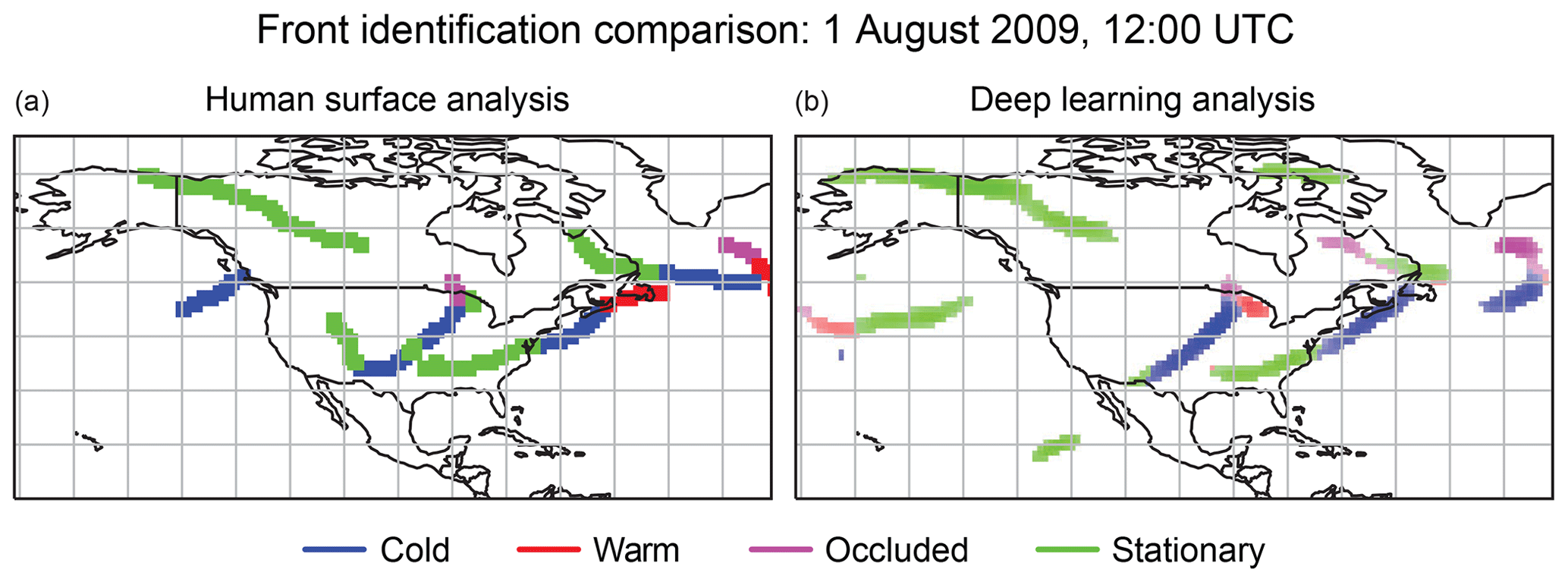
Figure 4Side-by-side comparison of CSB (a) and DL-FRONT (b) front boundaries for 1 August 2009 12:00:00. The CSB fronts were drawn three grid cells wide. The intensities of the colors for the different front types in the DL-FRONT image represents the likelihood value (from 0.0 to 1.0) associated with each grid cell.
4.2 Metrics
The trained network was evaluated by calculating the metrics discussed below for both the 2003–2007 training data and the 2008–2015 validation data. We combined the results for the four different front types to produce a two-category front/no-front dataset and produced metrics for the same two date ranges. The same region mask used for training was used when calculating the metrics.
4.2.1 Actual and predicted grid cell counts
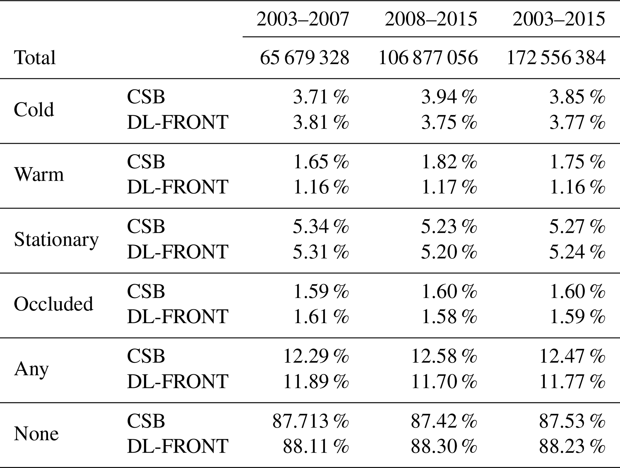
The percentage of grid cells in the five different types is shown in Table 1 for the CSB and DL-FRONT. In the CSB, the percentage of grid cells categorized as front is in the range of 12.3 %–12.6 % for the training and validation periods. The DL-FRONTS algorithm identifies fronts in 11.7 %–11.9 % of the grid cells. Thus, there is a slight undercount but little difference between the training and validation periods. The percentage of the different frontal types is similar between the CSB and DL-FRONT except for warm fronts, which are undercounted by DL-FRONT. Table 1 also shows that there is a major asymmetry between the front type categories, with ∼88 % of the grid cells falling into the no-front category.
Table 1Counts of CSB and DL-FRONT grid cells within the region mask over the training and validation time ranges and fraction of grid cells occupied by different front types.
4.2.2 Categorical accuracy
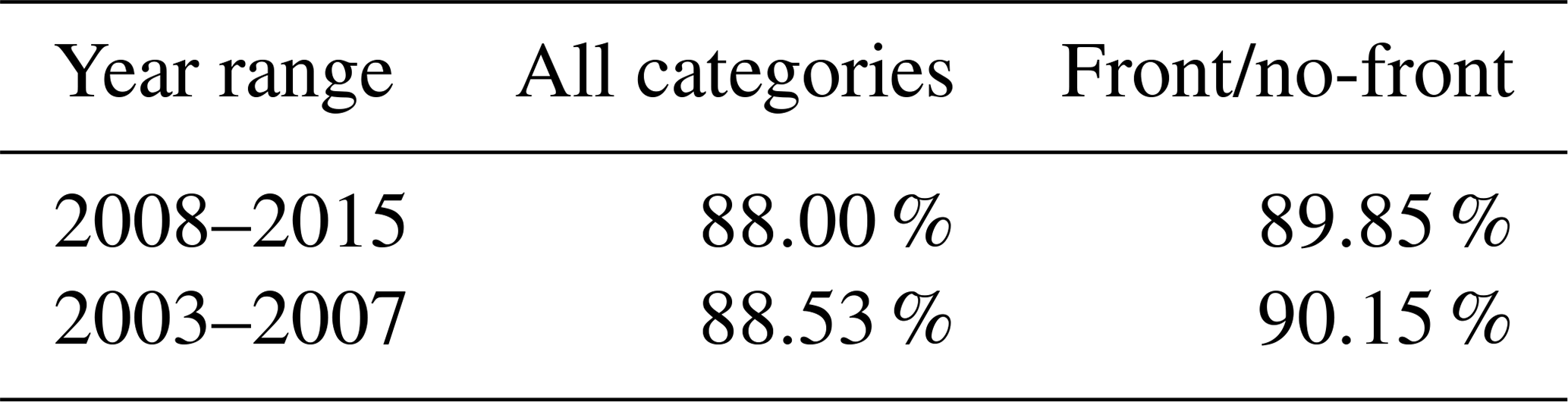
The categorical accuracy is a measure of the fraction of instances where the neural network predicted category matches the actual category for some set of samples. This is the sum of the diagonal elements of the confusion matrix (see below) divided by the total number of cells. The results for the full output and front/no-front output for the two time ranges are shown in Table 2. The results appear to indicate that there is no appreciable reduction in neural network performance with the validation dataset compared to the training dataset.
The large asymmetry between the no-front category and the other categories reduces the utility of this metric, since a network that identified all grid cells as falling in the no-front category would achieve a categorical accuracy of ∼87.7 % (the same values seen in the “None” column in Table 1). Comparison of the per-category counts in Table 1 shows that this is not the case.
Table 2Categorical accuracy values over the training and validation time ranges for the case where all categories are considered independent and the simplified front/no-front case.
4.2.3 Confusion matrices
Confusion matrix statistics were collected for both date ranges for the full results and the simplified front/no-front results. Table 3a and b show the full results presented as fractions of total cells for each front category and both date ranges. Table 4a and b show the front/no-front results as fractions of total cells for both date ranges.
The confusion matrices confirm the results found in Tables 1 and 2. The most prominent type of confusion is identifying a cell which is an actual front cell as no-front. This occurs at a similar frequency as the correct identification of an actual front cell. While this level of misidentification seems high, further analysis indicates that many of these erroneous classifications are due to differences in the location of fronts rather than not detecting the front. In addition, in those cases in which an actual front cell is identified as a front but of the wrong type, the mistyping is found in two clusters: confusion between stationary fronts and warm fronts and between stationary fronts and cold fronts.
Table 3(a) The confusion matrix as percentages of total grid cells for all front categories over the 2008–2015 validation time range. (b) The confusion matrix as percentages of total grid cells for all front categories over the 2003–2007 training time range.

Table 4(a) The confusion matrix as percentages of total grid cells for the simplified front/no-front categories over the 2008–2015 validation time range. (b) The confusion matrix as percentages of total grid cells for the simplified front/no-front categories over the 2003–2007 training time range.

4.2.4 Receiver operating characteristic (ROC) and precision–recall curves
The receiver operating characteristic (ROC) curve is a plot of the true positive rate (TPR) as a function of the false positive rate (FPR) as the threshold for a network output to qualify as positive is varied. The TPR is the number of correctly predicted positives divided by the number of actual positives, and the FPR is the number of incorrectly predicted positives divided by the number of actual negatives. ROC curves were developed for binary solutions, ones where there are only two categories, so the curves displayed here were produced using the simplified front/no-front categories.
Figure 5a shows the ROC curve for the DL-FRONT network for both the 2003–2007 training and 2008–2015 validation periods. The curves were produced by multiplying the no-front category likelihood values by a factor that varied from 0 to large enough that all grid cells were labeled as no-front. The multiplying factor is displayed next to the corresponding points on the curves.
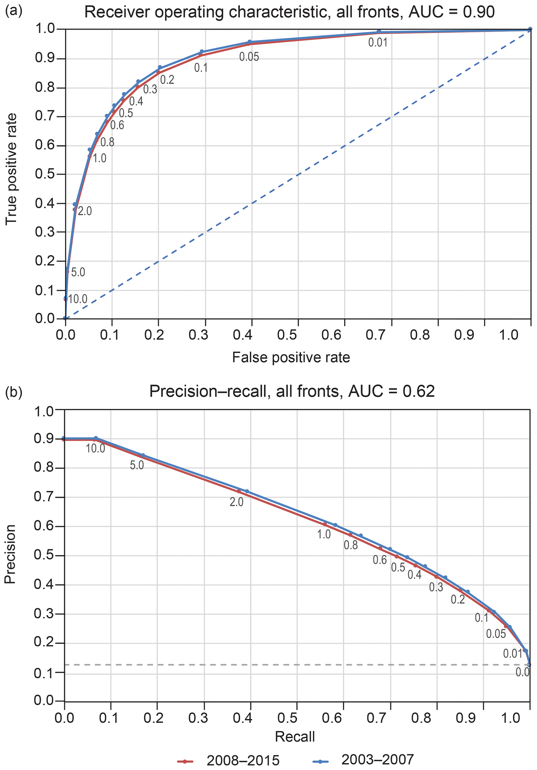
Figure 5Receiver operating characteristic curves (a) and precision–recall curves (b) for the simplified front/no-front categories over the 2008–2015 validation and 2003–2007 training time ranges.
An ideal ROC curve would rise with near infinite slope from the origin to a true positive value of 1 as the threshold is reduced from infinite (which causes all cells to be marked as no-front) to any finite value, then changing immediately to a slope of zero and remaining at a true positive rate value of 1 as the threshold is reduced to zero (which causes all cells to be marked as front). Such a curve has an area under the curve (AUC) of 1. The closer an ROC curve comes to that ideal, the better the overall performance of the network. A network producing random results would have an ROC curve like the blue dashed line in Fig. 5a, with the number of false positives matching the number of true positives for all threshold values.
The ROC curves (Fig. 5a) again confirm that the performance of the network on the validation dataset is quite similar to the performance on the training dataset. They also show that the native performance of the network (threshold value of 1.0) lies on the conservative side of the ROC curves, with a true positive rate that is relatively high while maintaining a small false positive rate. The AUC value of 0.90 is considered to indicate good system performance.
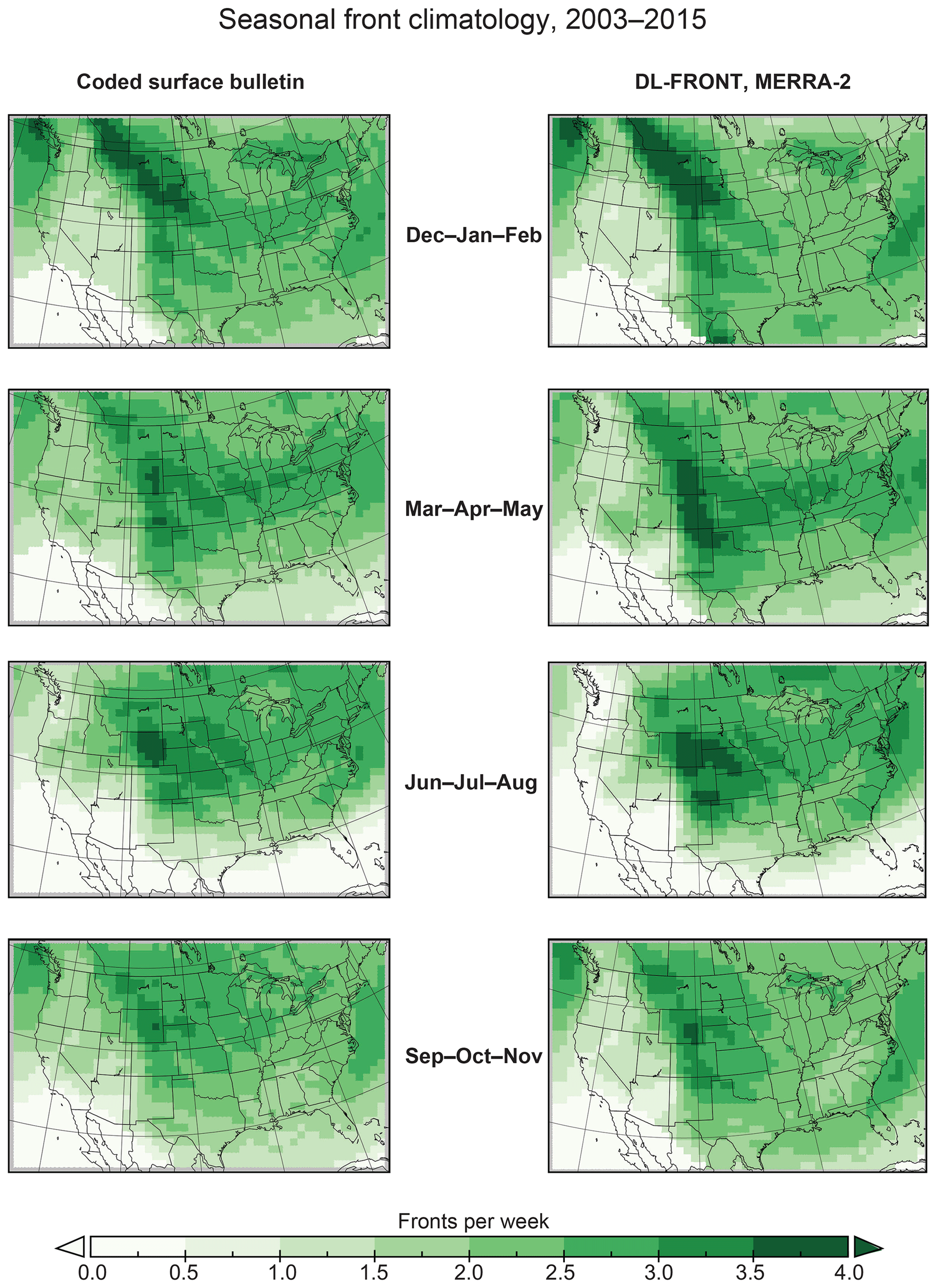
Figure 6Maps of seasonal front crossing rate climatologies (2003–2015) for the CSB and DL-FRONT datasets.
Precision–recall curves are another way to characterize the performance of binary machine learning solutions. In this case, the precision (the number of correctly predicted positives divided by the number of predicted positives) is plotted against the recall (the number of correctly predicted positives divided by the number of actual positives) as the threshold for marking a grid cell as positive is varied. The precision for the infinite threshold case cannot be measured, as the denominator will go to zero, so the precision for the largest practical threshold is typically reused for the infinite threshold case. An ideal precision–recall curve would have a precision value of 1 for all recall values. Precision–recall curves are considered to be less biased by large asymmetry between the categories, as opposed to ROC curves, which tend to present overly optimistic views of system performance when the categories are asymmetric.
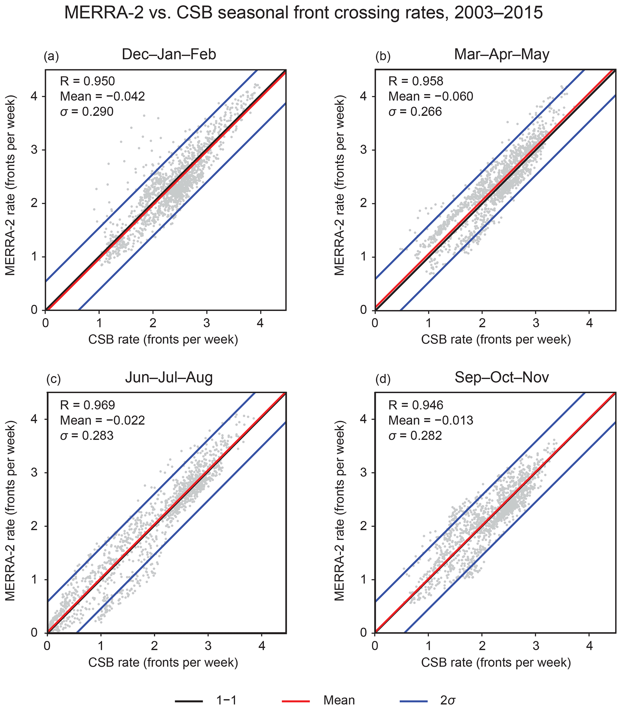
Figure 7Scatter plots comparing the DL-FRONT and CSB seasonal front rate climatologies over the CONUS-centered ROI.
Figure 5b shows the precision–recall curves for the validation and training datasets for the simplified front/no-front categories. The dashed blue line indicates the “no skill” random performance curve. If the categories were symmetric, the “no skill” level would be at a precision of 0.5. The curves are, again, almost identical, and the native network solution (threshold of 1) is in the region of the curve that maximizes both precision and recall. The network appears to be performing well.
The polyline extraction application was run to obtain front polylines from the full DL-FRONT front likelihoods dataset. The result was a front polyline dataset covering the same 2003–2015 time span as the CSB dataset. The CSB and DL-FRONT polylines were then used to calculate corresponding sets of monthly front crossing rates on the NARR Lambert Conformal Conic CRS 96 km × 96 km spatial grid. Monthly and seasonal front crossing rates were calculated for both datasets for each front type and for the simplified front/no-front case. The front crossing rates were used to calculate monthly and seasonal climatologies using the entire 13-year span. Figure 6 shows maps of the CSB and DL-FRONT MERRA-2 seasonal front/no-front rate climatologies for a rectangular region of interest (ROI) centered over the contiguous United States (CONUS). The use of this region minimizes edge effects produced by the uneven spatial coverage of the CSB dataset. The regions of zero rate in the southwest and southeast corners of the maps are the result of applying the mask shown in Fig. 2. The maps show a large degree of similarity between the seasonal front crossing rates calculated using the human-created and DLNN-generated fronts.
Figure 7 shows scatter plots comparing the values shown in each pair of maps in Fig. 6. Each scatter plot displays the one-to-one correlation line, a line displaying the mean of the differences between the paired DL-FRONT and CSB front crossing rate values, and a pair of lines that delineate ±2 standard deviations of the differences. The Pearson's correlation coefficient for each distribution is greater than 0.94 in every case, indicating a high degree of correlation. While most paired grid point values are within 10 % of each other, some pairs differ by considerably more. The ±2 standard deviation limits, which encompass 98 % of DL-FRONT MERRA-2 grid point climatology values, are ∼0.5 front crossings every week, compared to CSB climatology values centered around 2–3 fronts every week, indicating that some grid point pairs differ by about 20 % or more.
Kunkel et al. (2012) performed an analysis of the meteorological causes of daily extreme precipitation events at individual stations. One of their categories was fronts. Trained meteorologists categorized each event visually from a set of weather maps. They found that about half of all events occurred near fronts. In that study (led by the second author of this paper), the distance from event to front was not quantified because the judgments were all made visually. However, we estimate that an event within 300 km of a front would have usually been classified as a frontal event. There were 3191 frontal events for the period of overlap between that study and the MERRA-2 DL-FRONT data generated here: 1980–2013. For each of the 3191 events, the distance to the nearest MERRA-2 event was determined. Figure 8 shows the cumulative distribution function of the distances to fronts. Approximately 97 % of the events are within 200 km of a MERRA-2 front. The results are very similar for all seasons. While these results are not purely quantitative because of the “expert judgment” nature of the Kunkel et al. (2012) study, they do suggest that DL-FRONT is effective at identifying the “weather-producing” fronts.
Figure 9 compares the results of taking spatial averages of the CSB and DL-FRONT MERRA-2 monthly front/no-front rate climatologies over the CONUS ROI of Fig. 6. The spatial averages track each other quite closely, with the values always falling within ±1 standard deviation of each other.
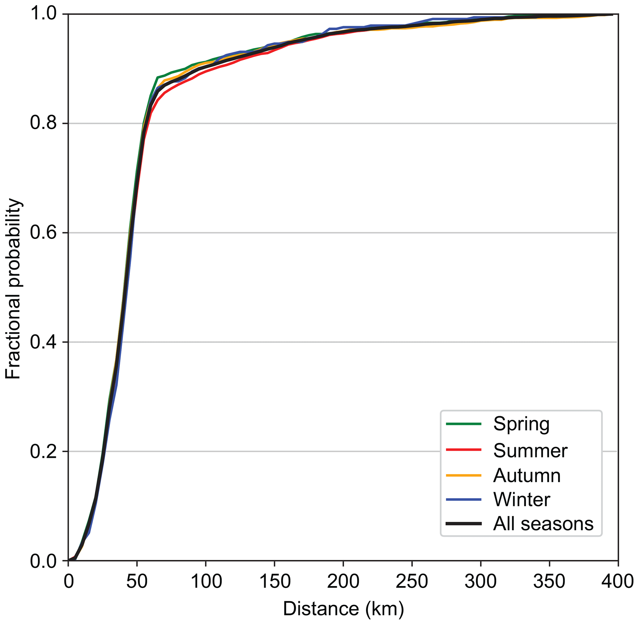
Figure 8The cumulative distribution of the number of extreme precipitation events caused by fronts from Kunkel et al. (2012) as a function of the distance to the nearest front identified by DL-FRONT in MERRA-2 for 1980–2013.
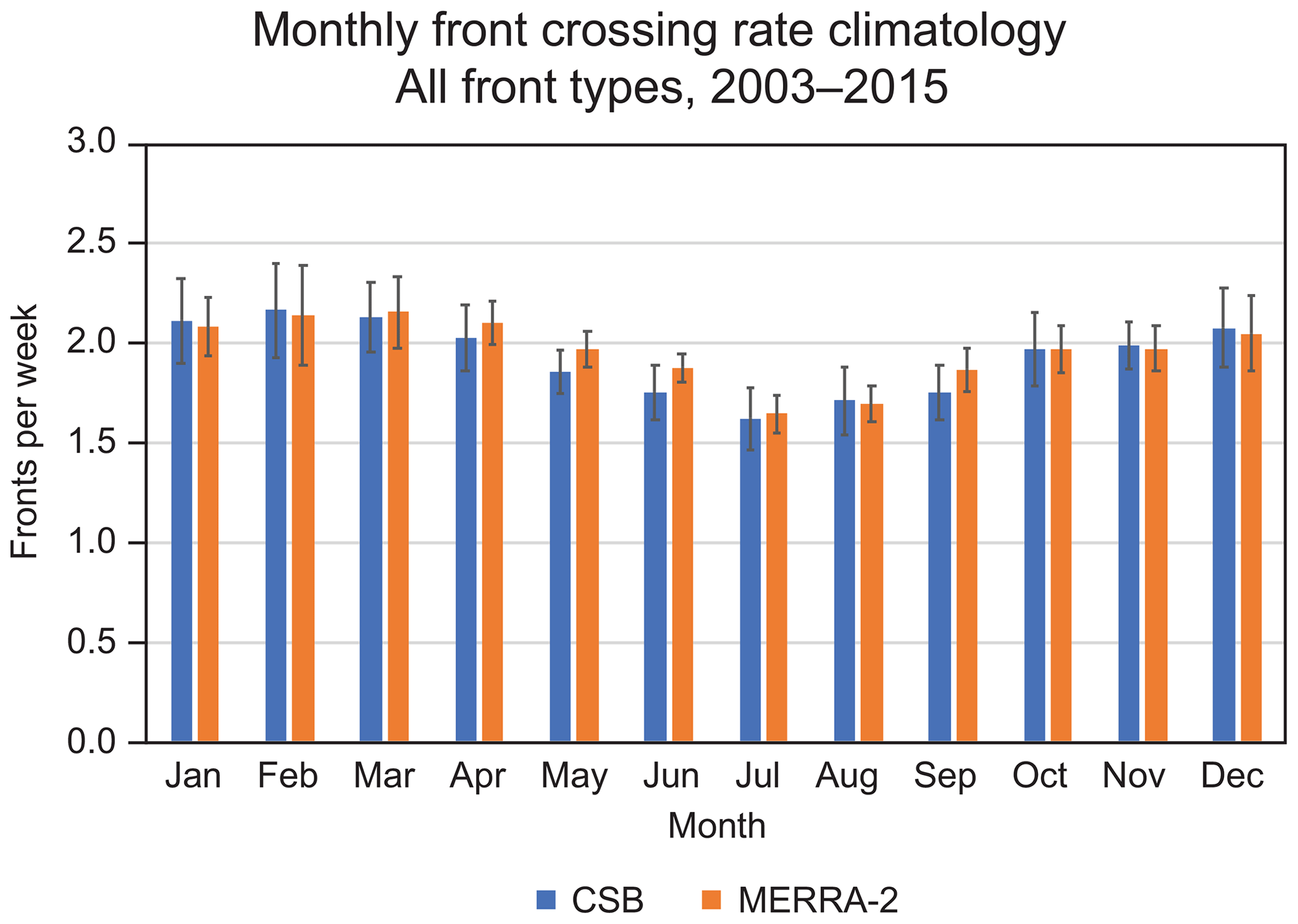
Figure 9Comparison of the front/no-front CSB and DL-FRONT MERRA-2 monthly front crossing rate climatologies spatially averaged across the entire CONUS ROI.
Temporal variability was assessed by averaging the monthly front/no-front crossing rates over the entire CONUS ROI. Monthly crossing rates were expressed as anomalies from the monthly climatology values. A comparison of the time series of monthly crossing rates (Fig. 10) indicates good agreement with an r value of 0.70 (p<0.01). Both time series have relatively low values during 2008–2010 with higher values on either side of that time period. However, the CSB time series has a statistically significant (p<0.01) upward trend while the MERRA-2 trend is essentially zero. Since 2012, the CSB has been higher than MERRA-2 in most months. The reasons for this are not known and beyond the scope of this study.
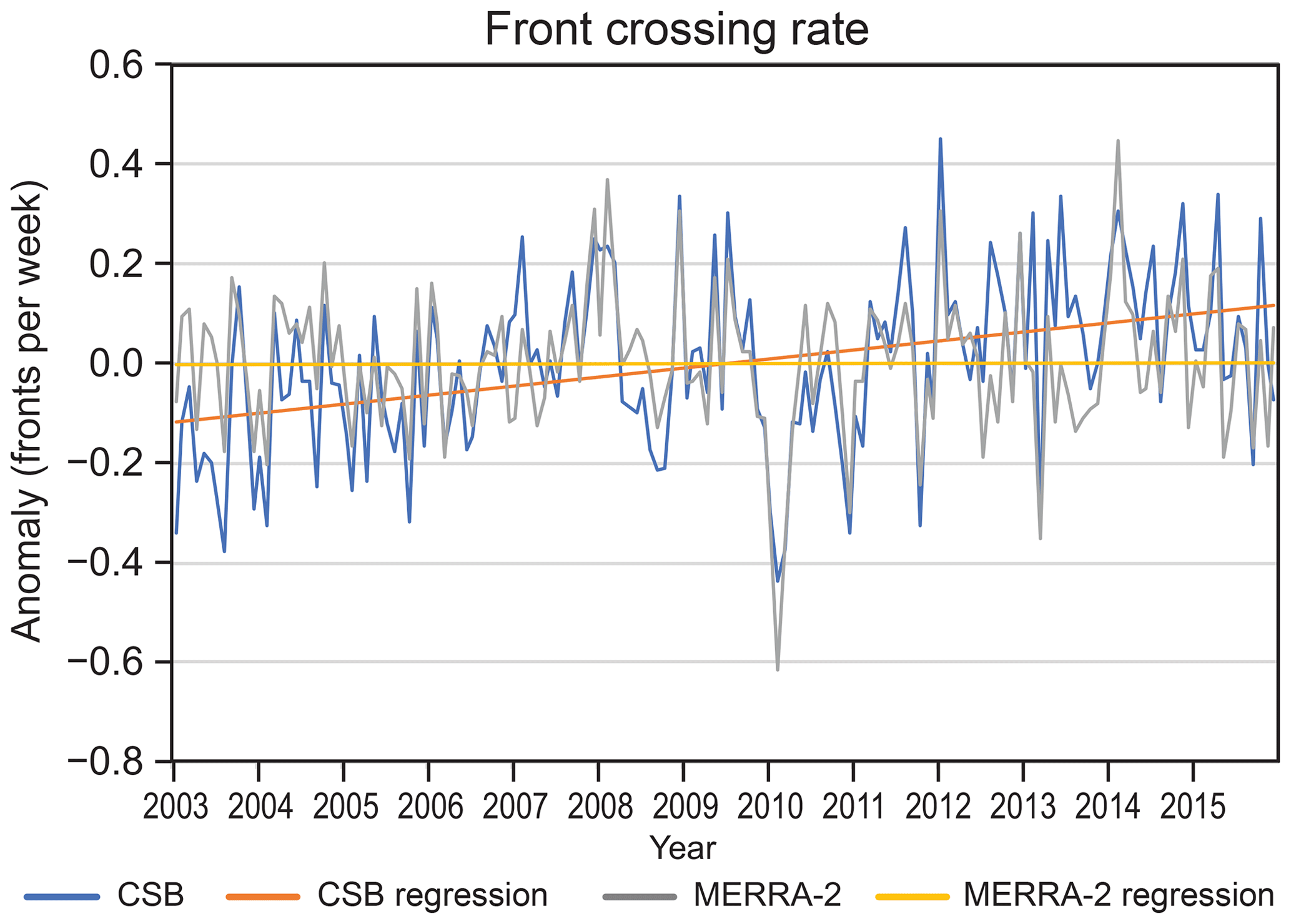
Figure 10Monthly time series of the domain-average frontal crossing rate anomalies for CSB and for MERRA-2 analyzed by DL-FRONT.
A two-dimensional convolutional neural network (CNN) was trained with 5 years (2003–2007) of manually analyzed fronts to develop an algorithm (DL-FRONT) for the automatic detection of fronts from surface fields of five atmospheric variables: temperature, specific humidity, pressure, and the two components of the wind vector. An analysis of the period 2003–2015 indicates that DL-FRONT detects nearly 90 % of the manually analyzed fronts over North America and adjacent coastal ocean areas. An analysis of fronts associated with extreme precipitation events suggests that the detection rate may be higher for important weather-producing fronts. Our immediate application for this algorithm is the detection of fronts that are associated with extreme precipitation. The superior performance for that subset of fronts gives us confidence that it is appropriate for application to our project needs.
One advantage of using deep learning methods to develop a fronts detection algorithm is that it is straightforward to add additional fields. Training the algorithm is computationally intensive, making it impractical to change the input fields often, but it does not require any fundamental restructuring of the problem. An additional advantage is that this approach can capitalize on future advances in the field of deep learning. One potential disadvantage is that the algorithm does not explicitly incorporate a physical understanding in the form of an equation, as most previous methods do. Thus, it is difficult to diagnose poor performance from fundamental principles.
Since DL-FRONT was trained on a North American dataset, its level of suitability for global applications is untested. However, the basic frontal structure of extratropical cyclones is global. On that basis, we expect that DL-FRONT will detect most fronts, and certainly most fronts accompanied by significant weather. However, where local topography plays a role in frontal orientation or other characteristics, its performance may be worse. An example of topographic influence is the front range of the Rocky Mountains where fronts often “hang up”. Noteworthy in this regard, our training dataset contains this region and it performs quite well in detecting these (Fig. 6). However, in other parts of the globe where topography affects front characteristics in other ways, this may not be the case. Early attempts to include a static elevation map in each input data grid did not provide any improvement in training, so its use was abandoned.
As noted earlier, Sanders (2005) argues that the identification of features with no horizontal density difference as fronts is not acceptable since density differences are required to produce key dynamical characteristics of ETCs. Since CSB will include some unknown percentage of such fronts and since our input fields include wind and pressure, DL-FRONT will not exclude the detection of such boundaries.
A comparison of the results of this method with one or more of the other methods that have been proposed and developed was beyond the scope of this project. The expanding number of approaches suggests that an intercomparison project of different algorithms would be potentially fruitful. A barrier to such a project is the lack of a curated labeled dataset that is global in extent. While users should be cognizant of its potential limitations, the CSB could serve that purpose for North America.
The data used in this study can be obtained through a few different channels. The MERRA-2 datasets used may be obtained from the NASA Goddard Earth Sciences (GES) Data and Information Services Center (DISC). The URL for the GES DISC is https://disc.gsfc.nasa.gov/ (last access: April 2019; Global Modeling and Assimilation Office, 2019). The specific subset of MERRA-2 used is the 2d, 1-Hourly, Instantaneous, Single-Level, Assimilation, Single-Level Diagnostics V5.12.4. We used the variables QV2M, SLP, T2M, U10M, and V10M remapped by bicubic interpolation to a 1∘ × 1∘ latitude–longitude grid.
The CSB dataset that we obtained from the NWS has been deposited in Zenodo in three different forms. It is available in its original ASCII form at https://doi.org/10.5281/zenodo.2642801, in JSON format at https://doi.org/10.5281/zenodo.2646544 (Biard, 2019a), and as rasterized data grids in netCDF format at https://doi.org/10.5281/zenodo.2651361 (Biard, 2019b). This dataset is available under the Creative Commons Attribution-ShareAlike 4.0 international license.
The fronts dataset produced by applying the trained DL-FRONT NN to the MERRA-2 dataset has been deposited in Zenodo. It is available in a number of different forms in multiple deposits. The front likelihood data grids and the one-hot version of the data grids in netCDF format are available at https://doi.org/10.5281/zenodo.2641072 (Biard and Kunkel, 2019a), the front polylines in JSON format at https://doi.org/10.5281/zenodo.2669180 (Biard and Kunkel, 2019b), and the front polylines as rasterized data grids in netCDF format at https://doi.org/10.5281/zenodo.2669505 (Biard and Kunkel, 2019c). These datasets are available under the Creative Commons Attribution-NonCommercial-ShareAlike 4.0 international license.
Various front processing and analysis artifacts, such as spreadsheets containing the values used to produce various graphs, have also been deposited in Zenodo. They are available at https://doi.org/10.5281/zenodo.2712481 (Biard and Kunkel, 2019d). This includes a movie showing the rasterized CSB fronts side-by-side with DL-FRONT front likelihoods for each 3-hourly time step in the year 2009. This dataset is available under the Creative Commons Attribution-NonCommercial-ShareAlike 4.0 international license.
KEK conceived the research goal of developing an automated means to find front boundaries and provided management and scientific supervision with support from Michael Wehner. JCB developed the software and carried out the bulk of the data processing, analysis, and visualization. JCB and KEK prepared the paper.
The authors declare that they have no conflict of interest.
This project took advantage of netCDF software developed by UCAR/Unidata (https://doi.org/10.5065/D6H70CW6). The work benefited from discussions with Evan Racah, Mr Prahbat, and Michael Wehner. Scott Stevens also provided valuable assistance.
This research has been supported by the Strategic Environmental Research and Development Program (grant no. W912HQ-15-C-0010) and by NOAA through the Cooperative Institute for Climate and Satellites – North Carolina under cooperative agreement NA14NES432003.
This paper was edited by William Hsieh and reviewed by Orhun Aydin and one anonymous referee.
Abadi, M., Agarwal, A., Barham, P., Brevdo, E., Chen, Z., Citro, C., Corrado, G. S., Davis, A., Dean, J., Devin, M., and Ghemawat, S.: TensorFlow: Large-scale machine learning on heterogeneous systems, available at: https://www.tensorflow.org/ (last access: April 2019), 2015.
American Meteorological Society Glossary of Meteorology: Front, available at: http://glossary.ametsoc.org/wiki/Fronts, last access: 27 March 2019.
Biard, J. C.: Coded Surface Bulletin (JSON format), Zenodo, https://doi.org/10.5281/zenodo.2646544, 2019a.
Biard, J. C.: Coded Surface Bulletin (netCDF format), Zenodo, https://doi.org/10.5281/zenodo.2651361, 2019b.
Biard, J. C. and Kunkel, K. E.: DL-FRONT MERRA-2 weather front probability maps over North America, Zenodo, https://doi.org/10.5281/zenodo.2641072, 2019a.
Biard, J. C. and Kunkel, K. E.: DL-FRONT MERRA-2 vectorized weather fronts over North America (JSON format), Zenodo, https://doi.org/10.5281/zenodo.2669180, 2019b.
Biard, J. C. and Kunkel, K. E.: DL-FRONT MERRA-2 vectorized weather fronts over North America (netCDF format), Zenodo, https://doi.org/10.5281/zenodo.2669505, 2019c.
Biard, J. C. and Kunkel, K. E.: DL-FRONT MERRA-2 weather front processing and analysis artifacts, Zenodo, https://doi.org/10.5281/zenodo.2712481, 2019d.
Bergstra, J., Breuleux, O., Bastien, F., Lamblin, P., Pascanu, R., Desjardins, G., Turian, J., Warde-Farley, D., and Bengio, Y.: Theano: A CPU and GPU Math Expression Compiler. Proceedings of the Python for Scientific Computing Conference (SciPy) 2010, 2010.
Berry, G., Reeder, M. J., and Jakob, C.: A global climatology of atmospheric fronts, Geophys. Res. Lett., 38, L04809, https://doi.org/10.1029/2010GL046451, 2011.
Catto, J. L., Jakob, C., Berry, G., and Nicholls, N.: Relating global precipitation to atmospheric fronts, Geophys. Res. Lett., 39, L10805, https://doi.org/10.1029/2012GL051736, 2012.
Chollet, F.: Keras: The Python Deep Learning library, available at: https://keras.io (last access: April 2019), 2015.
Cybenko, G.: Approximation by Superpositions of a Sigmoidal Function, Math. Control Sig. Syst., 2, 303–314, https://doi.org/10.1007/BF02551274, 1989.
Deng, L. and Yu, D.: Deep learning: methods and applications, Found. Trends® Sig. Process., 7, 197–387, https://doi.org/10.1561/2000000039, 2014.
Gelaro, R., McCarty, W., Suárez, M. J., Todling, R., Molod, A., Takacs, L., Randles, C. A., Darmenov, A., Bosilovich, M. G., Reichle, R., Wargan, K., Coy, L., Cullather, R., Draper, C., Akella, S., Buchard, V., Conaty, A., da Silva, A. M., Gu, W., Kim, G., Koster, R., Lucchesi, R., Merkova, D., Nielsen, J. E., Partyka, G., Pawson, S., Putman, W., Rienecker, M., Schubert, S. D., Sienkiewicz, M., and Zhao, B.: The Modern-Era Retrospective Analysis for Research and Applications, Version 2 (MERRA-2), J. Climate, 30, 5419–5454, https://doi.org/10.1175/JCLI-D-16-0758.1, 2017.
Global Modeling and Assimilation Office: MERRA-2 inst1_2d_asm_Nx: 2d,1-Hourly,Instantaneous,Single-Level,Assimilation,Single-Level Diagnostics V5.12.4, Goddard Earth Sciences Data and Information Services Center, https://doi.org/10.5067/3Z173KIE2TPD, 2019.
Goodfellow, I., Bengio, Y., and Courville, A.: Deep Learning, MIT press, Cambridge, MA, USA, 2016.
Hewson, T. D.: Objective Fronts, Meteorol. Appl., 5, 37–65, https://doi.org/10.1017/S1350482798000553, 1998,
Hinton, G. E., Srivastava, N., Krizhevsky, A., Sutskever, I., and Salakhutdinov, R. R.: Improving neural networks by preventing co-adaptation of feature detectors, arXiv preprint, arXiv:1207.0580v1 [cs.NE], 2012.
Huang, Y., Li, Q., Fan, Y., and Dai, X.: Objective Identification of Trough Lines Using Gridded Wind Field Data, Atmosphere, 8, 121, 2017.
Jenkner, J., Sprenger, M., Schwenk, I., Schwierz, C., Dierer, S., and Leuenberger, D.: Detection and climatology of fronts in a high-resolution model reanalysis over the Alps, Meteorol. Appl., 17, 1–18, https://doi.org/10.1002/met.142, 2010.
Kingma, D. and Ba, J.: Adam: a method for stochastic optimization, arXiv preprint, arXiv:1412.6980, 15, 2015.
Kolmogorov, A. N.: On the representation of continuous functions of many variables by superposition of continuous functions of one variable and addition, Dokl. Akad. Nauk SSSR, 114. 953–956, 1957.
Kunkel, K. E., Easterling, D. R., Kristovich, D. A. R., Gleason, B., Stoecker, L., and Smith, R.: Meteorological causes of the secular variations in observed extreme precipitation events for the conterminous United States, J. Hydromet., 13, 1131–1141, 2012.
Mesinger, F., DiMego, G., Kalnay, E., Mitchell, K., Shafran, P. C., Ebisuzaki, W., Jović, D., Woollen, J., Rogers, E., Berbery, E. H., Ek, M. B., Fan, Y., Grumbin, R., Higgins, W., Li, H., Lin, Y., Manikin, G., Parrish, D., and Shi, W.: North American Regional Reanalysis, B. Am. Meteorol. Soc., 87, 343–360, https://doi.org/10.1175/BAMS-87-3-343, 2006.
National Weather Service: Coded Surface Bulletin, Zenodo, https://doi.org/10.5281/zenodo.2642801, 2019.
Neilsen, M. A.: Neural Networks and Deep Learning, Determination Press, available at: http://neuralnetworksanddeeplearning.com (last access: 7 July 2019), 2015.
Parfitt, R., Czaja, A., and Seo, H.: A simple diagnostic for the detection of atmospheric fronts, Geophys. Res. Lett., 44, 4351–4358, https://doi.org/10.1002/2017GL073662, 2017.
Pedregosa, F., Varoquaux, G., Gramfort, A., Michel, V., Thirion, B., Grisel, O., Blondel, M., Prettenhofer, P., Weiss, R., Dubourg, V., Vanderplas, J., Passos, A., Cournapeau, D., Perrot, M., and Duchesnay, É.: Scikit-learn: Machine Learning in Python, J. Machine Learn. Res., 12, 2825–2830, 2011.
Sanders, F. and Hoffman, E. G.: A Climatology of Surface Baroclinic Zones, Weather Forecast., 17, 774–782, https://doi.org/10.1175/1520-0434(2002)017<0774:ACOSBZ>2.0.CO;2, 2002.
Sanders, F.: Real Front or Baroclinic Trough?, Weather Forecast., 20, 647–651, https://doi.org/10.1175/WAF846.1, 2005.
Schemm, S., Rudeva, I., and Simmonds, I.: Extratropical fronts in the lower troposphere – global perspectives obtained from two automated methods, Q. J. Roy. Meteorol. Soc., 141, 1686–1698, 2015.
Simmonds, I., Keay, K., and Bye, J. A. T.: Identification and climatology of Southern Hemisphere mobile fronts in a modern reanalysis, J. Climate, 25, 1945–1962, https://doi.org/10.1175/JCLI-D-11-00100.1, 2012.
Stull, R.: Practical Meteorology: An Algebra-based Survey of Atmospheric Science, University of British Columbia, Vancouver, British Columbia, Canada, 2015.
The Theano Development Team, Al-Rfou, R., Alain, G., Almahairi, A., Angermueller, C., Bahdanau, D., Ballas, N., Bastien, F., Bayer, J., Belikov, A., and Belopolsky, A.: Theano: A Python framework for fast computation of mathematical expressions, arXiv preprint, arXiv:1605.02688, 2016.
van der Walt S. S., Chris Colbert, S. C., and Varoquaux, G.: The NumPy Array: A Structure for Efficient Numerical Computation, Comput. Sci. Eng., 13, 22–30, https://doi.org/10.1109/MCSE.2011.37, 2011.
van der Walt, S., Schönberger, J. L., Nunez-Iglesias, J., Boulogne, F., Warner, J. D., Yager, N., Gouillart, E., and Yu, T.: scikit-image: image processing in Python, PeerJ, 2, e453, https://doi.org/10.7717/peerj.453, 2014.
Wong, K. Y., Yip, C. L., and Li, P. W.: Automatic identification of weather systems from numerical weather prediction data using genetic algorithm, Expert Syst. Appl., 35, 542–555, https://doi.org/10.1016/j.eswa.2007.07.032, 2008.