the Creative Commons Attribution 4.0 License.
the Creative Commons Attribution 4.0 License.
 | 12 Mar 2019
Influence of initial ocean conditions on temperature and precipitation in a coupled climate model's solution
Robin Tokmakian
Peter Challenor
This paper describes results of an experiment that perturbed the initial conditions for the ocean's temperature field of the Community Earth System Model (CESM) with a well defined design. The resulting 30-member ensemble of CESM simulations, each of 10 years in length, is used to create an emulator (a nonlinear regression relating the initial conditions to various outcomes) from the simulators. Through the use of the emulator to expand the output distribution space, we estimate the spatial uncertainties at 10 years for surface air temperature, 25 m ocean temperature, precipitation, and rain. Outside the tropics, basin averages for the uncertainty in the ocean temperature field range between 0.48 ∘C (Indian Ocean) and 0.87 ∘C (North Pacific) (2 standard deviation). The tropical Pacific uncertainty is the largest due to different phasings of the ENSO signal. Over land areas, the regional temperature uncertainty varies from 1.03 ∘C (South America) to 10.82 ∘C (Europe) (2 standard deviation). Similarly, the regional average uncertainty in precipitation varies from 0.001 cm day−1 over Antarctica to 0.163 cm day−1 over Australia with a global average of 0.075 cm day−1. In general, both temperature and precipitation uncertainties are larger over land than over the ocean. A maximum covariance analysis is used to examine how ocean temperatures affect both surface air temperatures and precipitation over land. The analysis shows that the tropical Pacific influences the temperature over North America, but the North America surface temperature is also moderated by the state of the North Pacific outside the tropics. It also indicates which regions show a high degree of variance between the simulations in the ensemble and are, therefore, less predictable. The calculated uncertainties are also compared to an estimate of internal variability within CESM. Finally, the importance of feedback processes on the solution of the simulation over the 10 years of the experiment is quantified. These estimates of uncertainty do not take into consideration the anthropogenic effect on warming of the atmosphere and ocean.
- Article
(14480 KB) - Full-text XML
- BibTeX
- EndNote


Uncertainty in climate models occurs due to various sources. Multimodel and single-model ensembles of varying size can give a rough estimate of the uncertainty in some quantity of interest or outcome in a 10-year period, the point in time at which the influences from the initial conditions are thought to reach a minimum (e.g., Branstator and Teng, 2012). Previous studies using fully coupled ocean–atmosphere–land coupled general circulation models (GCMs), such as Pohlmann et al. (2013), Smith et al. (2007), Yeager et al. (2012), Deser et al. (2012), Kay et al. (2015), Troccoli and Palmer (2007), Sriver et al. (2015), and Kröger et al. (2012), vary initial conditions in a variety of ways. The ensemble sizes are small (10 or less) in most of these studies, making it difficult to estimate a probability density function (pdf) for any model outcome. In some experiments (e.g., Yeager et al., 2012), all ensemble members are initialized with the same ocean, and it is the variation in the atmosphere and land components that uniquely determines an ensemble member. For example, Yeager et al. (2012) use 10 different days and/or differing hindcast runs for January of a specific year to initialize the atmospheric component for the 10-member ensemble, while Troccoli and Palmer (2007) use two different expressions of greenhouse gases (GHGs) for their 6-member ensemble. The one study (Kröger et al., 2012) that does modify the ocean's initial conditions only has three realizations of the outcomes. There are several larger member ensembles (Sriver et al., 2015) which vary the initial conditions of all the GCM components. Such a study makes it impossible to separate out the effects of one component's influence on the outcomes over the others. Kay et al. (2015) and Deser et al. (2012) vary only the atmospheric component. However, they all provide useful insight into the internal variability of a GCM.
A previous experiment that examines the uncertainty in submodel (e.g., models of mixing) process parameter values (Tokmakian and Challenor, 2014) tests and shows the usefulness of emulators as a method to expand the sampling space for the determination of uncertainty. A companion paper to this one, Tokmakian and Challenor (2019), examines the initial-condition uncertainty using an ocean-only model and related emulators, 10 years in the future, without considering feedbacks between the ocean and atmosphere. The results from this companion study show that after 10 years, the uncertainty in the near-surface temperature is on the order of ±0.4 ∘C, with 95 % of the spatial areas having an uncertainty of less than ±0.9 ∘C. In general, there is low uncertainty in the tropical regions and higher uncertainty in areas such as the Antarctic circumpolar current and western boundary currents, where there is high variability. The initial ocean state becomes less and less important in an ocean-only model as time proceeds, especially in the near-surface region of the ocean. The result is consistent with many studies, extending back to Stammer et al. (1996) and Tokmakian (1996), that show that surface fields of an ocean simulation are driven largely by the forcing of the atmosphere at the ocean's surface and, with no feedback, the initial conditions' influence on the solution decays in time. Stammer et al. (1996) and Tokmakian (1996), however, do not quantify the uncertainty. When there is no reaction of the ocean back to the atmosphere, its realism is dependent on the atmospheric forcing product used. Any perturbation in the initial fields decays with time, but as the study of Tokmakian and Challenor (2019) shows, a small, residual uncertainty remains.
In this paper, we take the next step using our set of experiments and examine how uncertainty in the ocean's initial conditions contributes to the uncertainty in various prognostic and diagnostic quantities (metric) of a coupled climate model. This model includes the feedbacks that occur between the ocean and atmosphere. We ignore anthropogenic effects. This is deliberate. This paper determines the uncertainty in 10-year predictions with a model in the absence of any anthropogenic effect as a baseline. This baseline is needed for future work with anthropogenic forcing included. Having the baseline is essential for seeing how additional uncertainty is introduced into the system by the anthropogenic component. The approach in this paper is to take a relatively small ensemble (30 members) and apply a statistical methodology to achieve a reasonable probability distribution of the uncertainty for a chosen metric. That is, for any given metric, we first determine a posterior probability distribution for an outcome, at a given time, using a 30-member GCM ensemble and robust statistical methods. In a separate but related analysis, we then examine the temporal evolution of the metric across the ensemble to ascertain where the uncertainty, arising from the initial-condition perturbation, produces predictable patterns of variability or more chaotic behavior. The two analyses have separate but related mathematical frameworks.
In a mathematical framework, first consider an ensemble of simulations with some outcome, y, at a time t, and where the outcome for each ensemble member (i) is defined as follows:
where yi is the estimate of the metric given by one member of a forward model ensemble with some set of initial conditions, xi. We assume that if a very large ensemble (many thousands) of simulations of the GCM could be conducted with different initial conditions, then the mean of those many simulations would converge on ytruth (assuming no bias in the model). The ϵ terms are random variables representing different sources of uncertainty: ϵinitial identifies the uncertainty related to the initial condition and the focus of this research.
In addition, there is another source of uncertainty that needs to be addressed, ϵnumerical, which is the uncertainty due to the numerical scheme and model structure, including the uncertainty due to missing dynamics. A GCM with a different structure and/or different process dynamics may have a different ϵnumerical that results in a different temporal variability with different amplitudes or phasing. Because the same GCM is being used for all ensemble members, the uncertainty ϵnumerical is the same for each ensemble member. Even when the same model is run on different computers (Hong et al., 2013), the outcomes are the same.
The initial-condition uncertainty over all possible initial conditions is defined as follows:
where N is the number of all possible initial conditions and is the mean of all .
The second mathematical framework describes the ensemble variability, temporally. For any one ensemble member i, then
yinternal is what is described as internal variability by many (e.g., Sriver et al., 2015). yt,seasonal and yt,trend are the portion of the signal due to seasonal forcing and any long-term trend that is present. T is the total time period for the simulation and t is time, making the first term on the right side the long-term mean for the simulation. In this framework, areas of similar patterns can be identified, but with each ensemble member having distinct phasing arising from the initial-condition perturbation. These areas of similarity may help with identifying regions that can be used for prediction.
The paper is structured to first describe the experiment and its components and data that are fundamental to the experiment. It is followed by showing the estimation of uncertainty for various outcomes (first framework, Sect. 3). To help understand how the uncertainty manifests itself temporally, Sect. 4 (second framework) explores time-varying aspects of the ensemble and how the initial-condition perturbation contributes to the phasing of similar patterns. The section also explores how one field may or may not have an influence on other fields given its uncertainty pattern. How the two frameworks jointly contribute to a better understanding of a model's evolution and usefulness in prediction is discussed. In addition, the question of how the estimates of uncertainty relate to other variances or uncertainty is also discussed. Finally, the last section summarizes the findings of the experiment described in this paper.
The experiment is briefly described in an overview here, with details in the following paragraphs. A schematic of the experiment, Fig. 1 illustrates the sequence of events that lead to the creation of a robust uncertainty estimate. An ensemble (Fig. 1a) of GCM simulations is created such that only the initial ocean conditions vary (sampled from a distribution derived from reanalyses products). The experiment is designed such that a decomposition (b) of the initial conditions will allow for a robust statistical determination of the uncertainty (2σic, Eq. 2) of some outcome (e). The uncertainty determination is achieved by relating the ensemble outcomes to parameters associated with the initial field (i.e., the principle component (PC) loadings). The relationship, referred to as an emulator, can then be used to estimate outcomes for initial conditions not used by the complex climate model or GCM (d). Thousands of possible outcomes from possible initial conditions can be estimated quickly and efficiently, resulting in robust uncertainty estimates for a particular simulator quantity. As this is a Bayesian perspective, there is no difference between aleatoric and epistemic uncertainty.
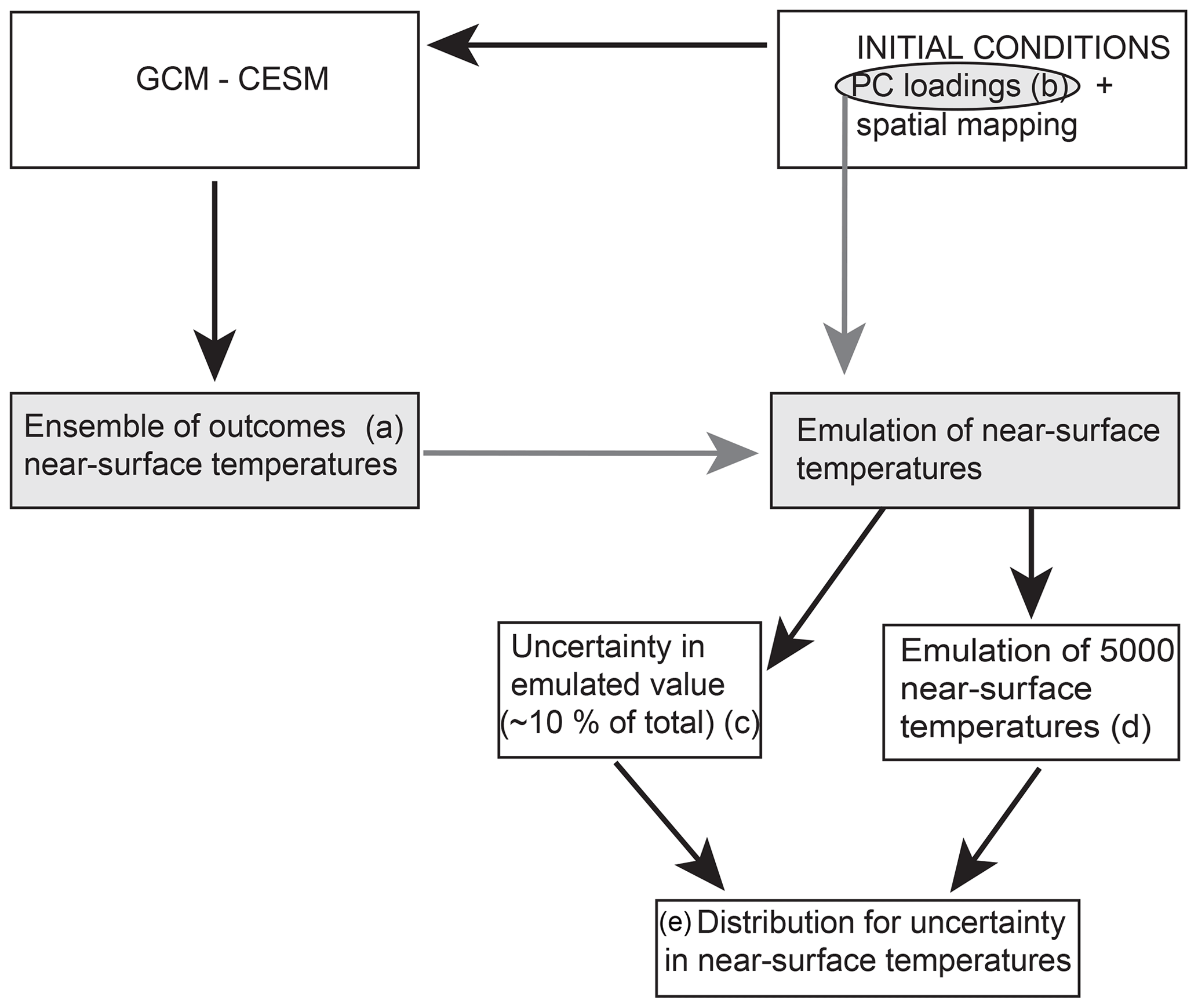
Figure 1Schematic describing the sequence of events undertaken in this study. The gray boxes and circle indicate the elements related to the emulator creation. The letters in parentheses are used in the text for identification.
We will also use the ensemble to quantify yinternal to understand temporal relationships to the uncertainty as described in Sect. 1 using Eq. (3).
In the following sections, we first describe the forward or GCM simulator and the source data for the initial fields. Next, the methods used for the sampling and creation of the initial fields and the emulator are explained. Two distinct statistical methodologies are used in this study to allow for the robust assessment of the uncertainty. The first method creates the distribution and sampling of initial value fields, while the second method is used to build a posterior distribution for some metric based on outcomes from a relatively small ensemble of forward simulations of the deterministic model. The posterior distribution is the basis for inferences about a metric's uncertainty.
2.1 Forward model
The forward model or simulator being used in this experiment is the Community Earth System Model (CESM) (Collins et al., 2006). With a horizontal resolution of approximately 1∘ (110 km), the vertical structure is represented by 60 levels, with the top 20 levels covering about 5 to 200 m. The ocean component model is POP2 (Smith and Gent, 2002), while the sea ice model is CICE (Hunke and Dukowicz, 2003; Bitz and Lipscomb, 1999). The atmospheric model in CESM is the Community Atmosphere Model (CAM5 Neale et al., 2010; Gent et al., 2010; Kiehl et al., 1998; Collins, 2001; Collins et al., 2006). Each ensemble member is restarted from the same previous spun-up simulation with a different perturbation of the initial ocean temperature field. A 30-day relaxation term on the temperature field nudges the model towards the initial field over the first month to reduce the shock of the introduction of the varied initial conditions to the simulation.
A total of 10 years of monthly averaged 3-D prognostic ocean fields (e.g., temperature, salinity, and velocity) along with 2-D monthly fields (e.g., sea surface height) are stored for later analysis. Similar prognostic quantities for the atmosphere are also stored on a monthly basis (e.g., velocities, temperatures, water vapor). Along with the prognostic variables, a large number of diagnostic quantities are available for analyses. The end result is an almost inexhaustible set of quantities which can be examined using the methods described in Sect. 2.4 to understand uncertainty in the model's processes due to differences in the initial conditions. For this paper we examine how perturbing the ocean's initial conditions affect the related fields of near-surface temperature (25 m) in the ocean, the surface air temperature, and the precipitation fields. Other fields, such as wind and current velocities and ocean overturning, may be explored in future research.
2.2 Initial fields
The initial fields are generated from a number of ocean reanalyses. Six ocean reanalyses contribute to the set of anomaly fields: the German Estimating the Circulation and Climate of the Ocean (GECCO; Köhl and Stammer, 2008), the Geophysical Fluid Dynamics Laboratory's Ensemble Coupled Data Assimilation (GFDL-ECDA; Chang et al., 2013), the Predictive Ocean Atmosphere Model for Australia (POAMA; Stone and Partridge, 2003), the European Centre for Medium-Range Weather Forecasting operational ocean reanalysis system (ECMWF ORAS4; Balmaseda et al., 2013), the University of Reading analysis (URA025.4; Valdivieso et al., 2012), and the Simple Ocean Data Assimilation (SODA; Carton and Giese, 2008). Anomalies are computed by differencing monthly fields from a reference reanalysis, URA025.4, for 2001 to the end of the particular reanalysis product (2009 or 2010). URA025.4, chosen as the reference field, has the highest resolution. Any long-term trend in the difference and any residual seasonal signals are also removed. This process results in an ensemble of 564 anomaly fields. Only potential temperature is used due to computational considerations.
The base initial field is extracted from one of the 20th century CESM large ensemble experiment data sets (Kay et al., 2015). For each of the 30 simulations, an anomaly or perturbation field is added to the base field creating the total initial value field. The method for determining the anomaly fields is described next.
2.3 Input distribution and sampling
Initial conditions include two sources of uncertainty. The first is the uncertainty related to observational measurement error combined with any reanalysis error. Uncertainty (or variance) also relates to the state of the ocean relating to yt,seasonal, yt,trend, and yt,internal in Eq. (3). For example, in some cases, the ocean may be in a temporal state that is more stable in the short term (for example, a strong El Niño) compared to a more unstable state (an eddy-rich region). These regions may be spatially distinct. Thus, the interannual to decadal uncertainty or variance depends upon the physical state of the ocean and how intrinsically variable a region is. This paper focuses on the first, the uncertainty that is related to the initial condition given the state of the ocean. At simulation time t=0, yt,seasonal, yt,trend, and yt,internal are the same at the large scales. All the anomalies are created from temporally consistent fields. Because we are sampling anomalies to add to a base field, the large-scale spatial structure of all initial fields is similar (e.g., the ENSO and seasonal phasing are the same).
Because a complex climate model cannot be run the number of times required to produce a believable and representative probability distribution, the set of all possible initial fields needs to be wisely subsampled. There are several possibilities for sampling strategies. One possible solution might be to create a large number of initial fields (O500) and sample a small number (30) from the distribution in a nonrandom way to ensure adequate coverage of the set of initial conditions. However, the problem remains of how to create a valid distribution for the outcomes, given only 30 members of some spatial field. It would be difficult, if not impossible, to find a regression relationship between the initial value spatial field and an outcome because of the size of the spatial field. However, such a regression is necessary to form a convincing posterior pdf. Kernel density methods (Silverman, 1986) might help but are unlikely to be informative with such small numbers.
A solution to the problem can be found if the initial-condition space can be reduced substantially to allow for the determination of such a relationship. The four-dimensional space (three spatial locations – latitude, longitude, depth – and also the sample number) can be decomposed into a set of principal components (PCs), thus reducing its dimensions. The PC loadings, rather than the full spatial fields, are sampled. The loadings are then used with the associated PC spatial maps to rebuild an initial value anomaly spatial field which, in turn, when added to the base field, is used to initialize the forward model. The sampled loadings are used as the independent variables (x) (rather than the fields themselves) for a multivariate regression process (the emulator; see Sect. 2.4, Fig. 1b) that relates the initial value fields to outcomes from the forward deterministic simulations (the GCM).
The size of the data set (described in Sect. 2.2) is large (76 641 spatial points by 30 levels by 564 samples) and it is necessary to divide the data set into regions before the decomposition. The regions are defined as the ocean basins: Indian, Pacific, Atlantic and Southern oceans.
Once decomposed, 30 samples are chosen from the 564 samples for each of 120 PCs using a Latin Hypercube scheme (McKay et al., 1979). Once the loadings are identified, they are combined with the appropriate spatial field to create a reconstituted initial anomaly field. These anomaly fields are then added to the base field (Sect. 2.2). In a companion paper, Tokmakian and Challenor (2019), details and examples of the sampling are given and we have chosen not to repeat the information in this paper.
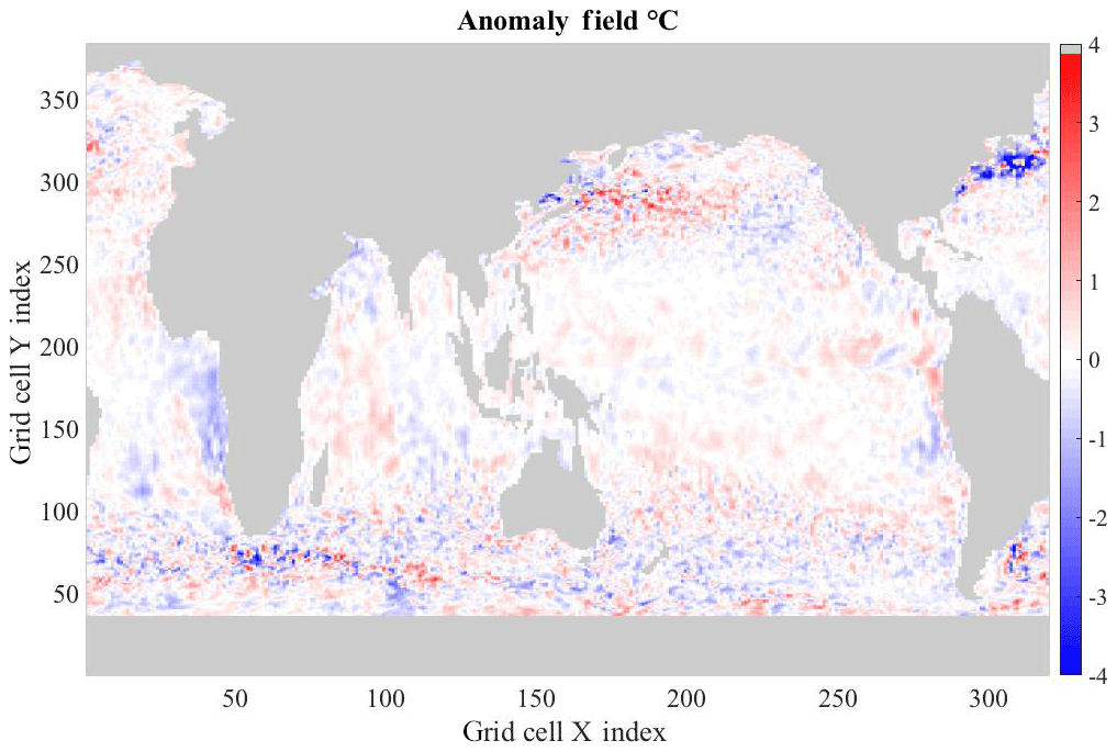
Figure 2 shows an example of one of the initial value anomaly temperature fields, reconstituted from the PCs. It contains large patches of similarly sized anomalies as well as areas that have changes on much smaller spatial scales. These are, generally, in the regions of the observed ocean that are highly energetic with much eddy activity and, hence, uncertainty. The reconstructed fields are similar to the original anomaly fields.
2.4 Posterior or outcome distribution
The method for creating the emulator, necessary for constructing the posterior uncertainty distribution, is a form of nonlinear regression, known as a Gaussian process regression. Given some input or independent variable (x), the value of the dependent variable can be determined. Having created the forward model ensemble with different initial conditions, sampled outcomes (where the outcome, y, is some metric of interest) form the set of the dependent variables for the uncertainty quantification. The statistical machinery conditioned on the relationship between the independent variable (the initial condition) and the dependent variable (the GCM outcome) define what is meant by an emulator. By providing the emulator with a large number of initial conditions, the posterior distribution is found for possible outcomes. In other words, the emulator allows for the determination of an outcome at locations where the simulator (the GCM) has not been run. Thus, through the use of the emulator, an ensemble for 5000 inputs can be created.
In its simplest form (two dimensions), the emulator is a regression fit of the input data (e.g., the loadings used to build initial conditions, Fig. 1b) to some output metric. Based on Gaussian process (GP) regression, an emulator has the advantage that it is more flexible than linear regression methods (and handles nonlinear relationships) and is as adaptable as neural networks but easier to interpret. GP methods also give estimates of the emulator uncertainty. A good, general reference for GPs is Rasmussen and Williams (2006). Challenor et al. (2010), Urban and Fricker (2010), Rougier and Sexton (2007), and Holden and Edwards (2010) provide examples of GPs for use with complex numerical models of oceanic and atmospheric processes. Previously, the authors used emulators based on GPs to understand the parameter space of imbedded physical models within geophysical deterministic models (Tokmakian et al., 2012; Tokmakian and Challenor, 2014). Full details of GP emulators are found in Appendix A.
Statistical inference about a quantity of interest for the simulator is carried out not by using the simulator but by using the emulator.
The 30 simulations of the forward model are run with varying initial conditions. After the simulation ensemble has been generated, an emulator, using the ensemble outcomes, is constructed such that it allows for the determination of a set of possible outcomes of sufficient size (5000). From the possible outcomes, an uncertainty pdf is generated. In the following sections, the maps of uncertainty for surface temperature, precipitation, and rain are described. Uncertainties are given as the 2σic value.
3.1 Uncertainty in the ocean's near-surface temperature field
The spatial map of the uncertainty, 2σic, for December of the 10th year for the ocean's near-surface (25 m) temperatures (Fig. 3a) shows large, cohesive, areas that have an uncertainty range of ±1 ∘C or greater (green-yellow areas). The uncertainty is largest in the tropical Pacific, with uncertainties reaching 10 ∘C. The amount of uncertainty is clearly a reflection of different phasing of the El Niño–Southern Oscillation (ENSO) signal in the various ensemble members. In areas where the ocean is more energetic, such as in the Southern Ocean and the western boundary currents, the uncertainty is reflecting both the intrinsic nature of the flow in these regions as well as differences induced by the initial conditions. In the discussion in Sect. 5, these two characterizations of the flow are explored.
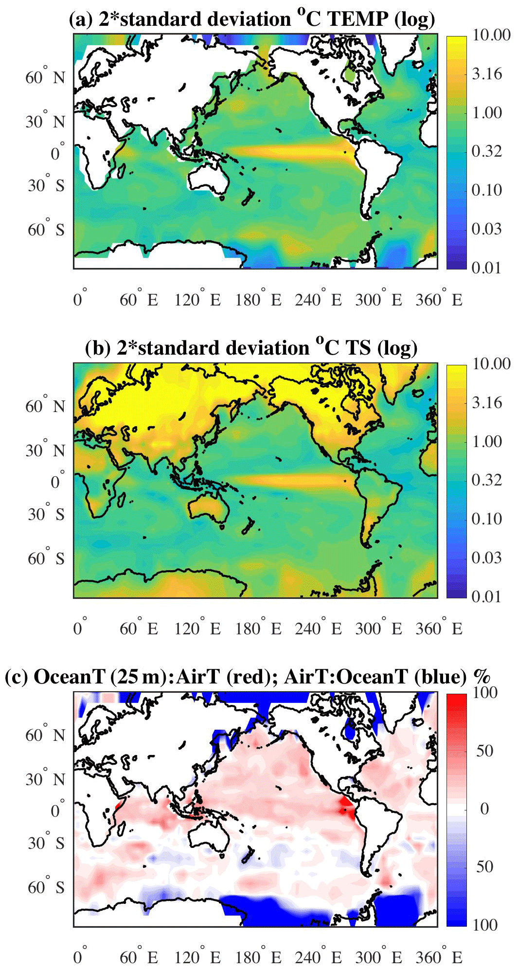
Figure 3Maps of 2 standard deviations for representing uncertainty (2σic) for December of the 10th year of the simulations in (a) ocean near-surface temperature field at 25 m and (b) surface atmospheric temperature in ∘C. (The shading is in terms of a log 10 value with tick marks labeled with unlogged values.) The ratio between the two fields is shown in (c), in which the ratio of the ocean temperature to the atmospheric temperature is given in red as a percentage. The inverse ratio is given in blue.
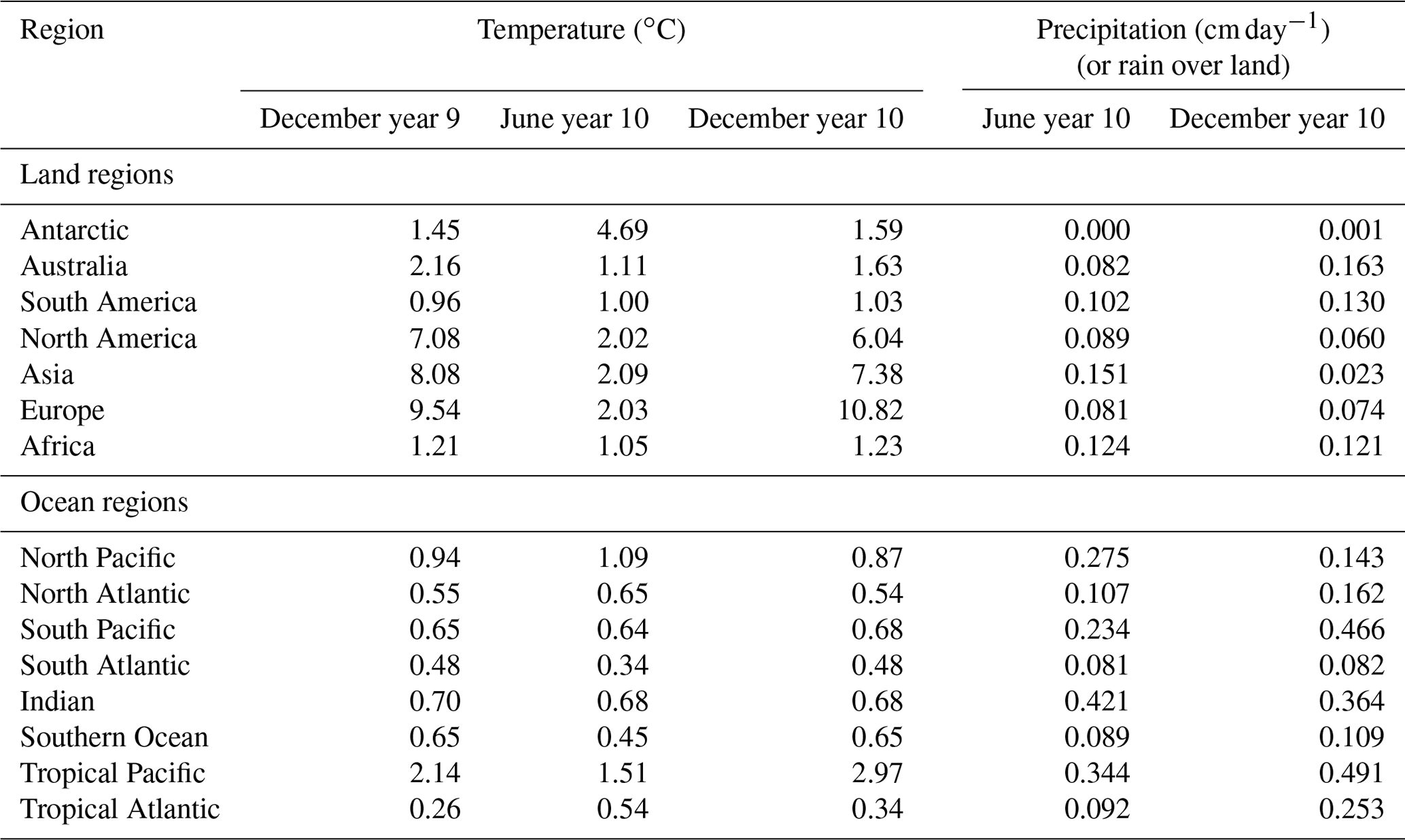
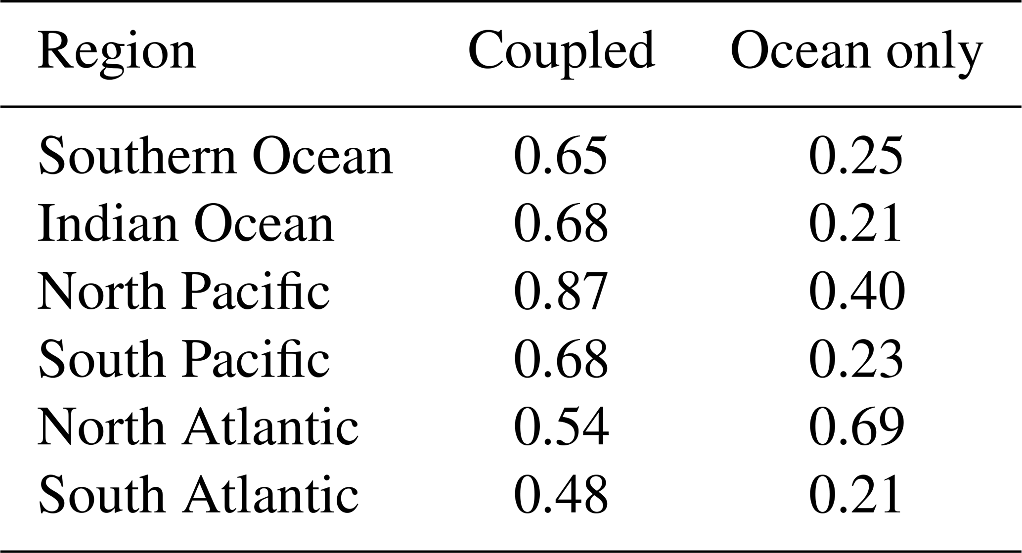
Basin averages for December year 10, outside of the tropics, north or south of ±10∘ N or S respectively, are as follows: North Pacific: 0.87 ∘C; North Atlantic: 0.54 ∘C; South Pacific: 0.68 ∘C; South Atlantic: 0.48 ∘C; Indian Ocean (including tropics): 0.68 ∘C; and the Southern Ocean: 0.65 ∘C (see Table 1, column 4). The tropical Pacific has the largest regional average at 2.97 ∘C. In contrast, the tropical Atlantic uncertainty is the smallest at 0.34 ∘C. For comparison, similar patterns of uncertainty can be calculated for any month of the simulation (not shown). The uncertainty maps for December of year 9 and June of year 10 exhibit similar spatial patterns as the December year 10 map. That is, the uncertainty in the tropical Pacific is the largest and the North Pacific uncertainty is larger than the North Atlantic, for example. The areal averages for these two additional months are also given in Table 1, columns 2 and 3 (ocean region). Generally, the two Decembers are of the same order for all regions. The June year 10 values are also generally of the same order. In the two tropical regions, the uncertainty in June is slightly higher than the December values in the tropical Atlantic sector and reversed for the tropical Pacific. In the Southern Ocean, the June uncertainty is slightly smaller.
3.2 Uncertainty in the atmospheric surface temperature field
The spatial map of uncertainty in the air surface temperature (December of the 10th year of simulation) field is shown in Fig. 3b. Over the ocean, as might be expected, the uncertainties are similar in size to uncertainties in the ocean temperatures at a depth of 25 m. Over land, especially at latitudes greater than 30∘ N, the uncertainty in the atmosphere is as large as or larger than the uncertainty in outcomes for the ocean's near-surface temperature. In the Southern Ocean, the atmospheric uncertainty is slightly larger than that for the near-surface ocean temperature.
The December uncertainty (2σic) values for land regions are listed in Table 1, column 4. The December average for year 9 and for June year 10 are also provided. As a consistency check. the two December uncertainty averages are of the same order for all regions. However, there is a difference in the average uncertainty values calculated for June of year 10 in the areas of the Antarctic, North America, Asia, and Europe. The differences between the two Decembers and June uncertainties imply that the winter months have a larger spread of temperatures in those areas than during summer.
The full extent of the differences in the uncertainties can be seen in a map of the ratios of the ocean temperature uncertainty to surface air temperature. Figure 3c illustrates the relationship between the ocean and atmosphere temperatures. The reddish areas are where the ocean temperature uncertainty is larger than the atmospheric temperature uncertainty and the areas where the atmospheric surface temperature uncertainty is greater are represented by the bluish colors. At latitudes greater than about 65∘ N or S (blue areas) the atmosphere uncertainties are greater by over 100 %. At the very eastern side of the tropical Pacific, the uncertainty in the ocean's temperature field is over twice the size of the atmospheric temperature uncertainty, hinting at more active oceanic processes in this region. In general, the Northern Hemisphere's ocean temperature uncertainties are on the order of 25 %–40 % greater than the atmospheric temperature (but still relatively small as compared to land temperature uncertainties). In the region between 30 and 60∘ S, there are areas where the atmospheric temperature uncertainty is larger than the ocean's and vice versa. But over this region, the percentages are relatively small (less than 20 %). If processes in both the ocean and the atmosphere are contributing to the uncertainties, then regions with equal contributions from both spheres (e.g., ocean or atmosphere) will have uncertainties of the same order. In regions where there is an imbalance (e.g., >25 %), then the processes related to the sphere (atmosphere or ocean) with the greatest uncertainties are dominant.
3.3 Uncertainty in atmospheric precipitation and rain fields
The uncertainty patterns of two related model fields, total precipitation (atmospheric component output) and rain (land component output), are shown in Fig. 4. The maps are for June (a, c) and December (b, d) of the 10th year of simulation. It can be seen, in the Northern Hemisphere, the spatial distributions of uncertainty are lower over the inner regions of the continents versus the coastal regions. In general, the tropical uncertainties are low. The June maps are similar in the Northern Hemisphere (Fig. 4a and c), while the December maps (Fig. 4b and d) differ from each other when comparing the land-based uncertainty over southern Africa, Australia and South America. The difference in the uncertainties for December are largely due to snow not being included in Fig. 4b for the Northern Hemisphere. In the Antarctic, the difference again is because most of the precipitation falls as snow.

Figure 4Maps of 2 standard deviations for representing uncertainty (2σic) for June (a, c) and December (b, d) of the 10th year of the simulations in (a, b) rain (land) field (cm day−1) and (c, d) total precipitation (cm day−1). (The shading is in terms of a log 10 value with tick marks labeled with unlogged values.)
In December, both the rain and precipitation maps show relatively large uncertainty for the west coast region of the United States, in the south central to northeastern regions of the United States, and over eastern Greenland. Over the tropical Pacific ocean, Fig. 4c and d, the region has relatively high uncertainty for precipitation in both June and December. Most of the uncertainty arises from the variability of the convective processes (as compared to the uncertainty map of large-scale precipitation, not shown).
The December area averages are listed in Table 1, column 6 and the June values are in column 5. For December, the average regional land values, given in the table, show the highest uncertainty for the regions of South America, Australia and Africa (dominated by the area in the Southern Hemisphere). Over land, the seasonal difference in uncertainty shows that, in general, it is the summer months with the larger uncertainty (December for Antarctic and Australia, and June for North America, Asia, and Europe). Over the ocean, the uncertainties in the Pacific also follow this pattern, with the North Pacific uncertainty higher in June than December and reversed for the South Pacific. The reason for the tropical Atlantic's difference in the seasonal uncertainty is unknown, and needs further investigation that is outside the scope of this paper.
The atmosphere–ocean coupled system is so complex that it is difficult to determine cause-and-effect relationships. In the experiment, the ocean fields are perturbed over the full model, rather than at just one location, which complicates how to perform a cause-and-effect analysis. In an effort to understand how the 30 simulations are similar (or not) to each other and how ocean patterns relate to land patterns, a maximum covariance analysis (MCA) (e.g., Bretherton et al., 1992; Frankignoul et al., 2011) is performed for several regions of the model's domain. Others (e.g., Li et al., 2012) have used other methods to find correlations between a specific ocean location and land areas. Such methods are comprised due to the smaller scales of variability over land. The MCA method filters out these smaller scales. In this section, we are considering the mathematical framework as described with Eq. (3).
Prior to the analysis, a seasonal cycle (determined by averaging monthly values for each simulation) and a long-term trend (determined via linear regression) are removed from the fields for each of the 30 simulations. In this temporal analysis, ϵnumerical is included in the anomaly. The signal removals are done to highlight the interannual relationships in the data and what we are referring to as yinternal. MCA is designed to extract dominant patterns of variability and gives the percentage of covariance described by the patterns. Mathematically, given two data sets, X and Y, of size m×t and n×t, where m and n are the size of the spatial field and t is the time sampling, then the covariance matrix σ is as follows:
where U and V are the optimal, maximum patterns of covariance (or eigenvectors of Cxy) and Cxy is the covariance matrix. The percent covariance for the kth mode is defined as
Monthly fields for years 2 through 10 are included in the analysis. For each simulation, a separate MCA is performed, resulting in spatial maps for each mode along with associated time series, scaled to allow for comparison between land and ocean values. All analyses within this section are performed using the ocean temperature fields at 25 m and the land surface air temperature field, except for the last section, where the precipitation over land replaces the land temperature field. Stationarity is assumed over the period of the model simulation. The discussion for the North Pacific explores the analysis extensively to illustrate, in detail, how maps of the differences in ensemble members can be summarized. The discussions for the North Atlantic and tropical Pacific relationships are limited to just the summary figures because the details of how these are created are similar to the North Pacific analysis.
4.1 North Pacific
Figure 5 shows the first spatial mode (U over the ocean and V over land) for all 30 simulations using North Pacific near-ocean temperature fields and North America land surface temperature. In the top left corner is the simulation number. The percent of covariance (, Eq. 5) is in the bottom left corner for each simulation, representing the amount of covariance explained by the pattern. The maps are oriented such that each ocean pattern is positively correlated with all the other maps. That is, the sign of the maps (and associated time series) for a simulation are reversed when the majority of the ocean region's correlation value signs do not match 15 or more of the other simulations' sign orientation at the same location. The ocean patterns of the first mode for most of the simulations are similar, with positive values along the eastern edge of the basin and negative values to the west. The pattern is very similar to the Pacific Decadal Oscillation (PDO) spatial pattern found using observations of sea surface temperature (Mantua et al., 1997). It also allows for the exploration of how the land temperatures relate to similar or different ocean conditions. For example, in some of the 30 simulations (1, 2, 4, 7, 8, 15, 20), the region south of approximately the US–Canadian border is positive, while in other maps (3, 17, 21, 24, 27, 28, 30) that pattern is reversed. The different responses of the land temperatures given the ocean temperatures field in a similar state suggests that it would be difficult to use the ocean's state as a predictive guide for the land temperatures.
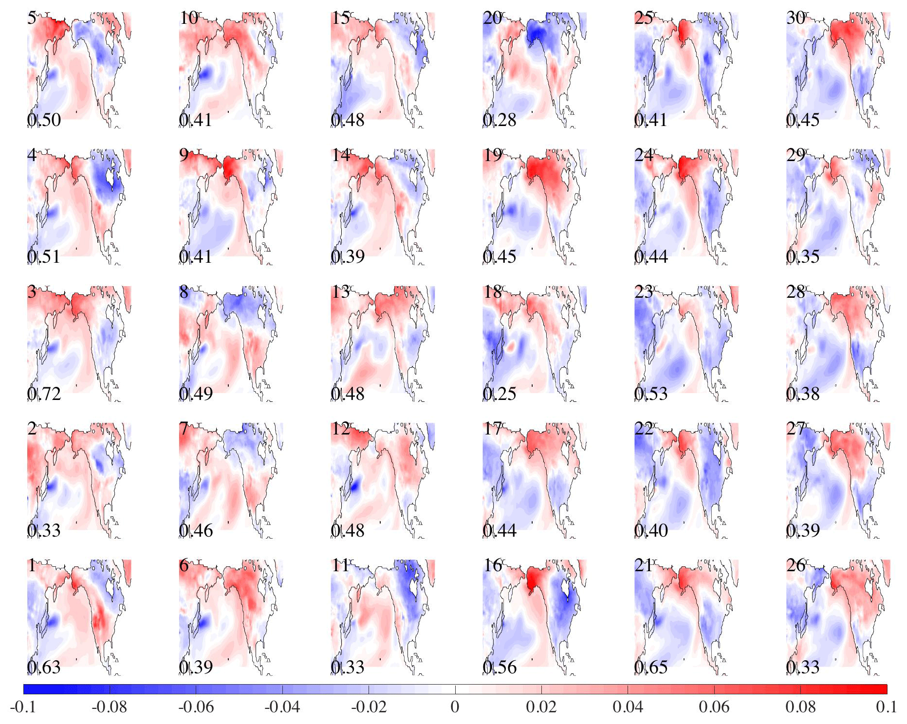
Figure 5MCA between ocean temperature at 25 m depth and land surface temperature. North Pacific Mode 1 for 30 simulations. Number in left-top corner is model number. The bottom-left-corner number is the percentage of covariance explained by pattern.
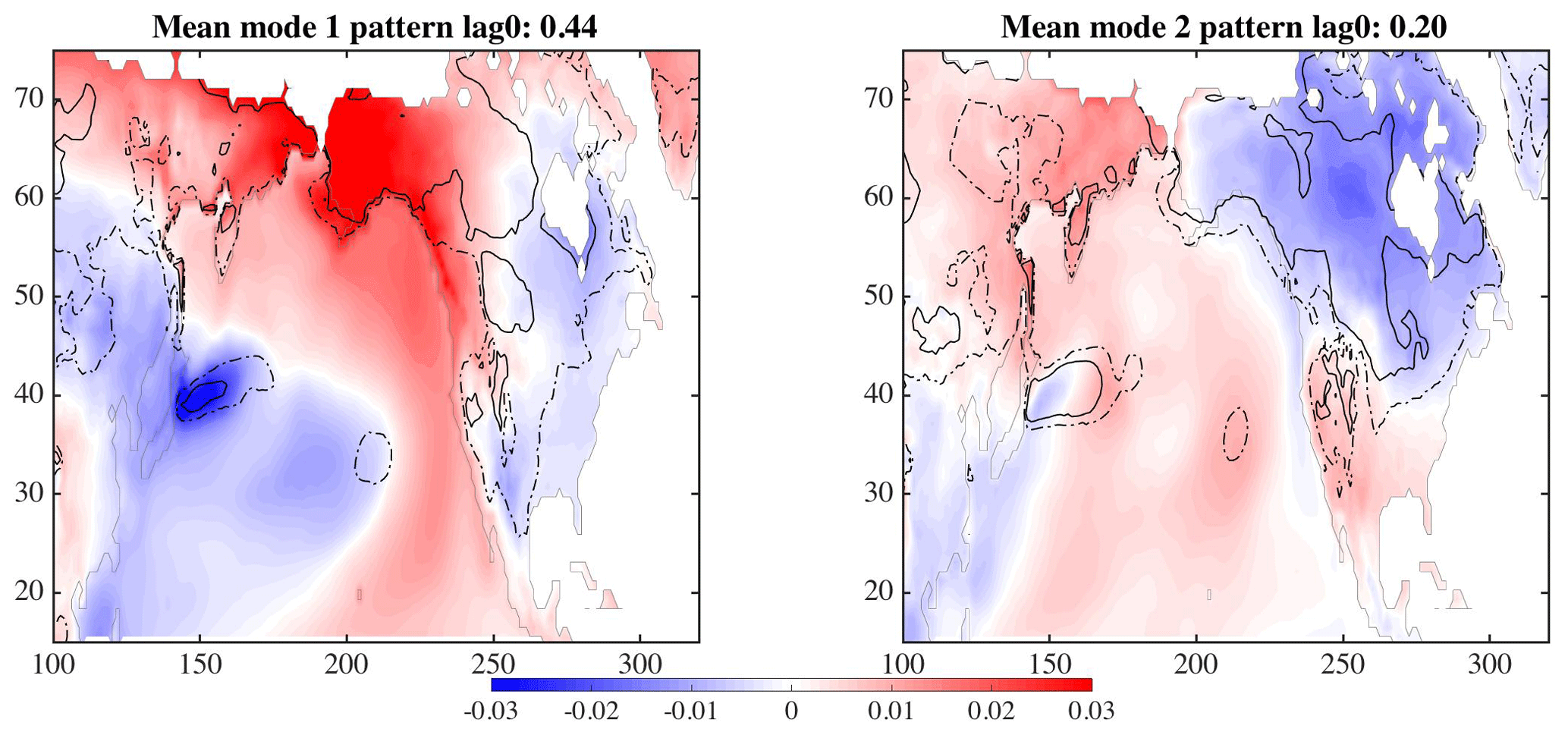
The mean and variance of the 30 maps shown in Fig. 5 for the first two modes are displayed in Fig. 6. The color represents the mean of the 30 maps, while the variance between the maps is shown as the dashed and solid lines (contours are 0.0008 for solid and 0.0004 for dashed lines). The largest uncertainties are in the regions of the Kuroshio Extension in the western Pacific Ocean, where different model simulations will have different paths for the current, and a location at about 35∘ N, 210∘ E. The land temperatures (concentrating on North America) have much greater uncertainty in northern Canada and the area west of the United States Rockies than in the eastern region of the United States. The area between 55 and 45∘ N along the west coast of North America also has relatively low variance for both the first and second modes, with respect to the eastern area. The low variance can be interpreted to mean that given a pattern, such as that seen in the North Pacific, the land temperatures, with low variance, respond similarly across all ensemble members and may be predictable.
The time series of these two modes for each of the areas – ocean (UTX) and land (VTY) – are shown in Fig. 7. The ocean series are on the left and the land series on the right. The first mode is in the top row and below is the second mode. The simulation run number is along the bottom, with time on the y axis. Within the ellipses, both the ocean and land regions for the first mode generally show a positive amplitude, but with the land time series much more variable. The first mode time series suggests a low-frequency signal on the order of 5 years. The time series show the signal of the dominant pattern in a different phase. The second mode's time series are much more complicated, again with the land series more variable. These plots also show how each of the 30 simulations, with perturbed ocean initial conditions, results in variation of the phasing of the interannual signal.
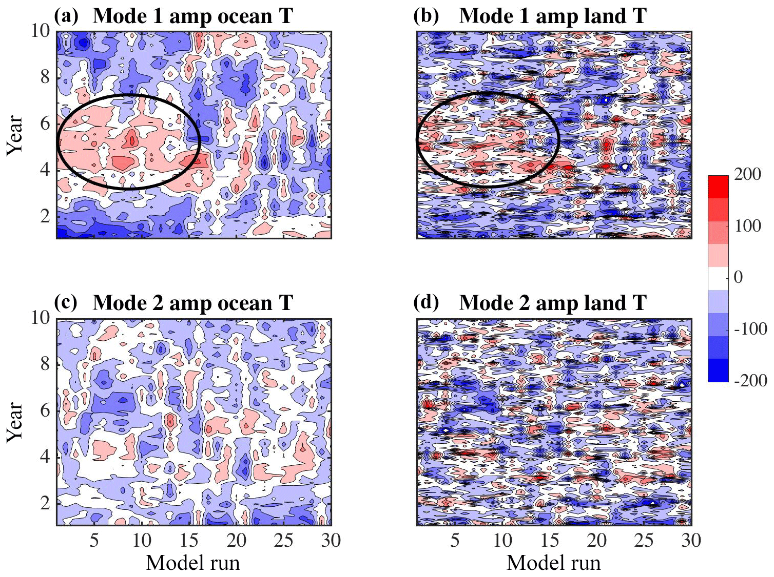
Figure 7Time series for MCA analysis associated with maps in Fig. 5 for modes 1 (a) and 2 (b), with ocean time series in column 1 and land time series in column 2. The model numbers are along the x axis with time on the y axis. The ellipses are used for identifying a region of interest in the text.
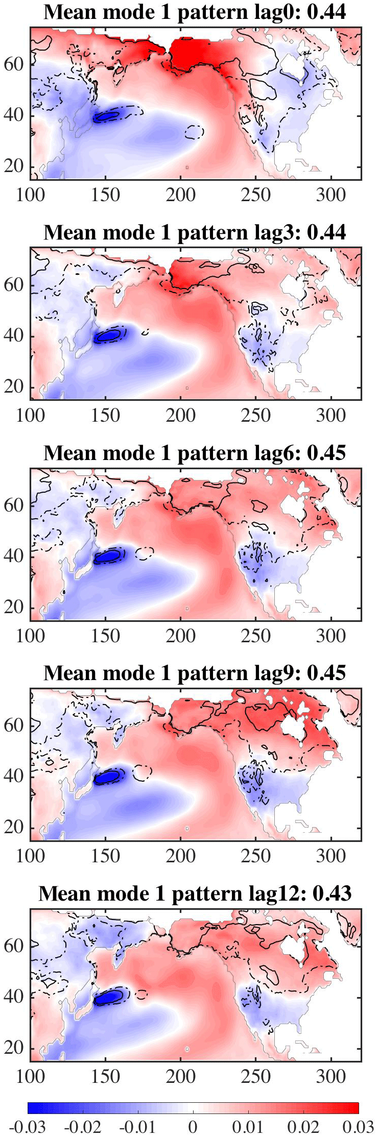
The previous paragraphs describe the analyses of the data at zero lag between the ocean temperatures and land temperatures. The same analysis can be done for lags of 3, 9, and 12 months. The spatial patterns of the mean and variance over 30 simulations (Fig. 8) shows that as the lag increases, the area of the largest uncertainty (dashed and solid lines) over North America is reduced over the 12 months. The analyses show that the North Pacific ocean temperature field increases its influence over the land temperature as the time difference progresses.
4.2 North Atlantic
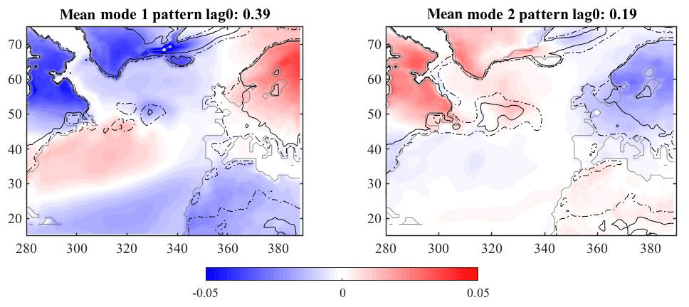
A similar MCA analysis can be performed for the North Atlantic ocean temperature with European land temperatures. Figure 9, resembling the well known (Hurrell et al., 2013) North Atlantic Oscillation (NAO) pattern, shows the mean pattern of covariance for modes one and two overlaid with the contours of variance. At zero lag, the relationship between the ocean and land temperatures is similar in the magnitude of covariance explained to that seen in the Pacific. There is relatively high variance (represented by the dashed and solid lines) over all 30 simulations in the Scandinavian region and low variance between simulations over northern Africa, Britain and Spain. The second mode also shows large variance between simulations over the ocean, meaning that there is not one ocean pattern over all simulations that can be used to describe the covariance patterns between the ocean and land temperatures. Covariance maps computed when lagging the land by several months behind the ocean do not result in substantially different patterns.
4.3 Tropical analysis
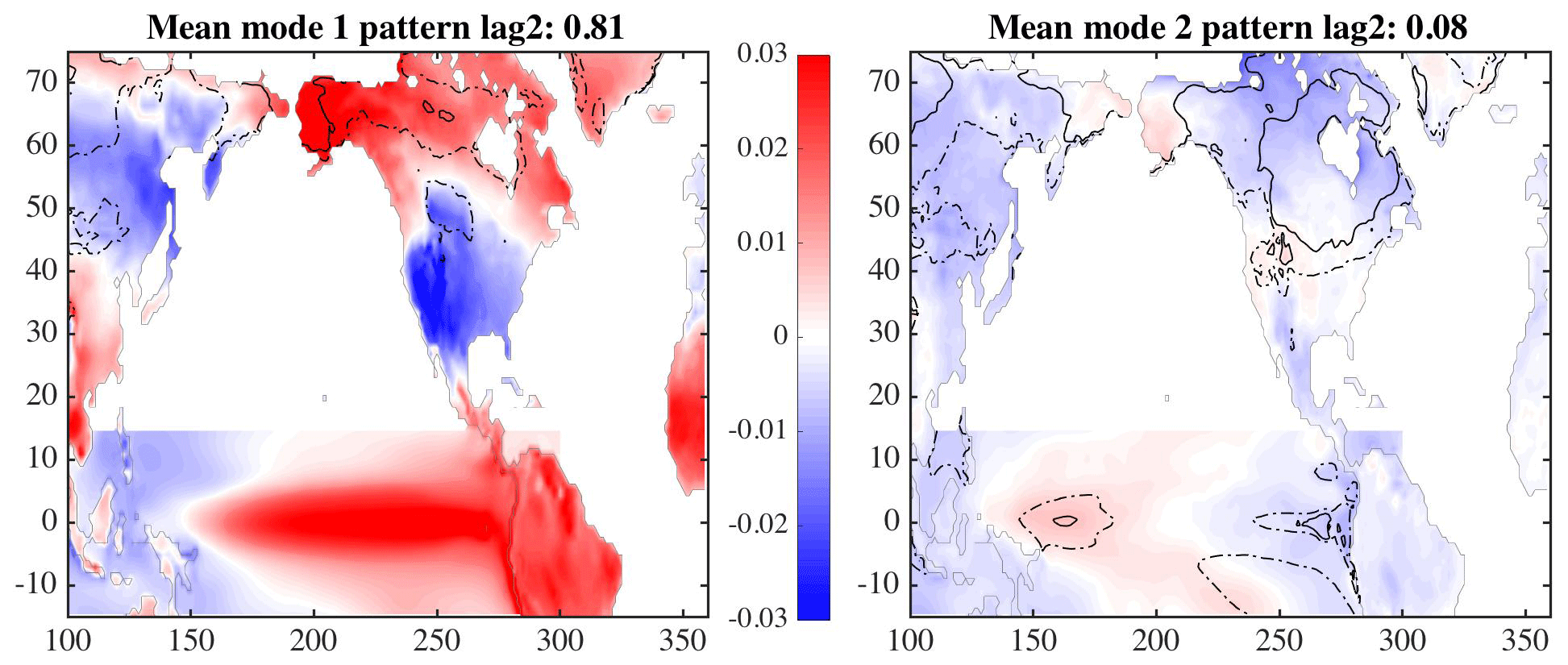
The tropical Pacific ocean temperatures, when analyzed with the land temperatures (Fig. 10), show a primary mode that explains 81 % of the covariance between the two fields. Rather than show many versions of the pattern at different lags, only the pattern at a lag of 2 months is shown (the patterns for other lags are similar). The variance (shown by the dashed and solid contours) is the lowest over all 30 simulations for this lagged period and the percent of covariance is the highest. Spatially, the variance is lowest for the United States region and increases northward into Canada. This pattern is consistent with the analysis of van Oldenborgh et al. (2012) (their Fig. 9b), showing ENSO teleconnections (note that the method of analysis differs, as well as the model configurations). The large areas with relatively low covariance values over the land show that the tropical ocean is influencing large areas of North America much more than the midlatitudes in the Pacific (see Sect. 4.1). A similar analysis using the tropical Atlantic rather than the tropical Pacific only explains 40 % of the covariance over Europe, similar to the midlatitude Atlantic percentage. This analysis is consistent with others such as Rodríguez-Fonseca et al. (2016) and Davey et al. (2014).
4.4 Precipitation analysis
To evaluate how the Pacific Ocean's near-surface temperatures influence the precipitation field over North America, an MCA is performed twice, once using the tropical Pacific Ocean temperatures and the second time using the area north of 15∘ N. The results are shown in Fig. 11. There is low variance across the 30 simulations in the interior of the continent in the analysis when using the tropical Pacific (Fig. 11a) for the mapping. The maps indicate that the tropical Pacific covaries in these simulations with the land temperatures to a degree twice as much as the North Pacific region (0.76 vs. 0.37 covariance values), which is in agreement with previous work. However, Fig. 11b suggests that the North Pacific midlatitude region does contribute to the uncertainty and the unpredictable nature of the land precipitation due to the high land variance between the simulations exhibited given a similar ocean temperature map.

The goal of this research is to understand how uncertainty (2σic) manifests itself in an ensemble of simulations based on the same numerics but differing only in the initial ocean conditions, the differences having been introduced by perturbations that represent our ignorance in the initial conditions. In Sect. 3 spatial maps of this uncertainty for various quantities for a given time (December) (Figs. 3 and 4) are produced, and in Sect. 4, the evolution of the initial conditions was analyzed in terms of yt,internal. Included in the analysis of the simulator ensemble was how the ocean temperatures influence land temperatures and precipitation (Sect. 4). Below the relationship to the simulator's internal variability (yt,internal) and how the uncertainty defined by 2σic can be used jointly to assess prediction possibilities is provided.
Secondly, we discuss what the maps of initial-condition uncertainty (2σic) mean with respect to a similar experiment without feedbacks between the ocean and atmosphere.
5.1 Uncertainty introduced by initial conditions
5.1.1 Internal variability
To understand how the uncertainty, 2σic, introduced by perturbing the initial conditions, relates to the internal variability of the system (yinternal, Eq. 3), the following is computed. From each of the 30 model simulations, a long-term mean and the seasonal cycle are removed from the surface air temperature field, y. The standard deviation is then found for the Decembers over all simulations and all years. December fields are used because we are making a comparison to the estimate for the uncertainty in December of year 10. Equation (6) represents the computation for the standard deviation, Z. One might think of this internal variability as the variability within an individual simulation.
where ym,n represents a monthly spatial field; is the mean of each simulation, n; m is the month in the model simulation from 1 to 120 (10 years); and n represents the simulation run or model number from 1 to nt, where nt=30. Further, let md equal the month of December (i.e., k=12, 24, 36, etc.), with 10 being the total number of Decembers per simulation. It is again noted that the uncertainty, 2σic, arising from ϵinitial in Eq. (1) is separate from yinternal as defined in Eq. (3) and the variance of yinternal is approximately the same for all members of our sample.
The field, shown in Fig. 12a, represents an estimate of the average variability in surface air temperature exhibited by the CESM simulator and shows twice as much Z′ as defined above to give an approximate 90 % confidence interval. The map represents what we refer to as the average internal variation of a quantity (in this case, temperature) across the simulations. Any model biases between the ensemble members have been excluded from the calculation (i.e., the standard deviation is calculated separately for each simulation and then averaged over all the simulations). The assumption is made that because all the simulations are using the same numerical code, with the only difference being a unique perturbation of the ocean's initial conditions, the variance represents the underlying variability due to the dynamics. The mapped variance is in contrast to the uncertainty seen in Fig. 3b, which represents the differences in phasing of signals between the simulations.

Figure 12(a) Represents the uncertainty within the simulations (“internal”, Z′) for surface air temperature over all Decembers. (The shading is in terms of a log 10 value with tick marks labeled with unlogged values; compare to Fig. 3b.) (b) Ratio temperature uncertainty in Fig. 12a (Z′) and Fig. 3b (Z*).
The map given in Fig. 12a shows, in general, an enhanced variability over the higher latitudes in surface air temperature. The temperature variability is much higher over land than over the ocean, as expected. Over the ocean, there is relatively high variability in the surface air temperatures in the tropical Pacific, and in regions of the Gulf Stream Extension and Kuroshio Extension (currents flowing northwestward of Cape Hatteras and Toyko, respectively) where the currents are highly variable.
To compare the estimate, Z′, with the estimate of uncertainty between the simulations shown in Fig. 3, ratios have been computed and are displayed in Fig. 12b (call this field Z*). The scale is in terms of percentages. In the reddish areas (), the ratio is computed as , while the blueish areas () show the inverse . Only in a few areas, such as along Antarctica and in the Greenland Sea, is the internal (or within-simulation) uncertainty greater than the between-simulation uncertainty. The relative uncertainty from introducing perturbations in the initial ocean fields is strongest at the high latitudes and in the tropical Pacific. The tropical signal is due to the phasing of the ENSO processes. It is noted that the sample size for the “within” or internal variability (O100) is much smaller than the sample size for the initial-condition uncertainty (O1000). Longer runs of the simulator would address the sample size difference, however, we did not have the computer resources available.
5.1.2 Comments related to the ocean-only ensemble
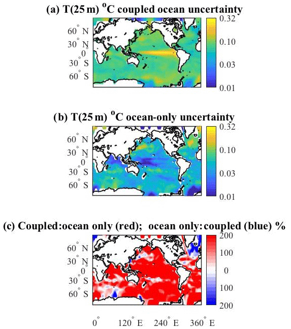
In a previous, related, experiment (Tokmakian and Challenor, 2019) the response to perturbing the initial ocean conditions without feedback processes between the ocean and atmosphere is examined. In the experiment, all 30 ensemble members of the ocean- or ice-only components of CESM are forced with the same atmospheric reanalysis product. Figure 13b shows the uncertainty field for the ocean temperature at 25 m for the December field of year 10 in the ocean-only ensemble. The ocean-only field is compared to the same field from the coupled ensemble, Fig. 13a (a repeat of Fig. 3a). Figure 13c is the ratio of Fig. 13a (red shades) to Fig. 13b (blue shades). Generally, the coupled response field is higher than the ocean-only ensemble uncertainty field (see Table 2), most notably in the tropical Pacific. As discussed above, the high tropical uncertainty is due to the phasing of the tropical signal in the coupled simulation. The ocean-only ensemble temperature uncertainty indicates slightly larger values for the areas centered about 55∘ N, 320∘ E in the North Atlantic, in the Kuroshio Extension region of the North Pacific, and parts of the Southern Ocean. An explanation for these enhancements has not been discovered. We suggest that in these regions the feedbacks between the ocean and atmosphere may dampen the variability of the ocean's temperature.
To look in detail at the differences between the two ensembles and to help in understanding the role of feedbacks in the simulations, the differences between pairs of monthly maps are summarized in Fig. 14 for ocean temperature at 25 m. Let , where X represents the spatial field for a month from the coupled ensemble and Y represents the same for the ocean-only ensemble. In all cases the atmospheric initial conditions are the same. In each pair, both the ocean-only and coupled members have the same ocean initial conditions. For each simulation, , the average difference for a given year is calculated. Table 3 column 2 gives the average over the 30 pairs for each year and column 3 is the standard deviation over the 30 pairs. The values show a steady increase in the spread through year 8, and then a small drop in year 9. The variance across the ensemble (column 3) indicates that for the first 5 years the spread increases and between years 6 and 9 the variance is approximately the same.

Figure 14Yearly averages of pair differences between monthly ocean temperature derivatives vs. pair differences , where X is the coupled simulation and Y is the ocean-only simulation. The color indicates the year, and each dot represents an ensemble pair.
Table 3Average mean differences () and average mean derivative () (∘C).
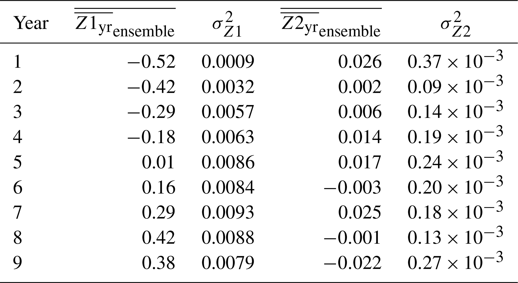
The second quantity calculated from the simulation outcomes is the difference in the temporal derivative, , where “it” represents the month. The average of these derivative values is then computed for each year, . Table 3 column 4 lists the averages over the 30 pairs for each year, with twice the ensemble standard deviation given in column 5.
vs. is plotted in Fig. 14. Each color represents a different year and each dot represents a different simulation pair (30 for every color). From bottom to top, it is clear that the differences show, as time progresses, the two ensembles diverging as increases, confirmed by column 2 of Table 3. Looking left to right in the figure, the spread of does not have a trend over time (summarized in column 4 and 5 of Table 3). Generally, is more positive than negative. The values of in time can be interpreted to mean that the feedback processes within the CESM model account for, on average, 0.008 ∘C globally (average of the over 30 models and 9 years). And after 9 years, the feedback contributes to about 0.4 ∘C globally (average of at 25 m over 30 models).
5.2 Two distinct uncertainty quantities
There are two distinct uncertainty (or variance) quantities described in this paper. The first relates to the initial conditions (Sect. 3, Eq. 1) and the second relates to the relationships between two metrics (Sect. 4) (e.g., temperature and precipitation) and how predictable one metric is given the other. The following paragraphs expand on the meaning of these two uncertainties.
The uncertainty represented by the variance contours in Figs. 5 and 9–11 allows us to make a statement about how well the metric over land (i.e., temperature or precipitation) is knowable, given the ocean's near-surface temperature pattern. For example, from Fig. 10a, with high confidence, all the models, no matter what the initial conditions are, will produce a similar ENSO-like pattern. The phasing of the ENSO signal may differ, as shown by the high uncertainty values in the tropics in Fig. 3b. And if the state of the tropical ocean is known and if a perfect model existed, there would still be significant uncertainty in the over land surface air temperatures in the regions at high latitudes in Canada and Alaska.
However, we do not have perfect knowledge of the ocean, and therefore an additional uncertainty, ϵinitial, is introduced by the perturbation of the initial conditions. If North America is used as an example, the yellow-orange area extending down into the United States in Fig. 3b illustrates the additional uncertainty.
We can use an equation with the same framework as Eq. (1) to describe the combination of these two uncertainties. Let y1 be the first metric, such as ocean temperature, and let y2 represent the second metric, for example land temperature.
where ϵinitial and ϵnumerical are as described in Eq. (1) and ϵpredictability is a third uncertainty related to the influence of one field on another.
The MCA maps, shown in Fig. 5, give a sense of understanding the land uncertainty (ϵpredictability) assuming low variance over ocean regions of the dominant pattern. The between-model uncertainty (ϵinitial) gives a sense of how important it is to know the state of the ocean. So, while it is well known that the tropical Pacific state reduces the ϵpredictability in temperature over large land areas, it is also clear that small perturbations in the ocean's initial field lead to relatively large ϵinitial in the outcomes, including the phasing of dynamical processes, such as ENSO.
This paper has described the results of an experiment that perturbed the initial conditions for the ocean's temperature field of the CESM with a well defined design. The experiment resulted in a 30-member ensemble of CESM simulations, each of 10 years in length. We estimated two types of uncertainty: (i) a robust estimate of uncertainty in a metric (temperature or precipitation) at a location and (ii) an estimate of uncertainty over land dependent upon the state of the ocean (MCA analysis).
Using outcomes of temperatures and precipitation from each ensemble member combined with statistical machinery known as an emulator, spatial maps of uncertainty have been calculated for air surface temperature, precipitation, and the ocean's near-surface temperature (25 m) fields for year 10 of the simulations. Basin averages, outside the tropics, for the uncertainty in the ocean temperature field range between 0.48 ∘C (Indian Ocean) and 87 ∘C (North Pacific). The tropical Pacific uncertainty dominates due to the different phasing of the ENSO signal. Over land areas, the regional averages vary from 1.03 ∘C (South America) to 10.82 ∘C (Europe). Similarly, the regional averages in precipitation vary. In general, both temperature and precipitation uncertainties are larger over land than over the ocean.
The MCA analysis for several regions showed how the ocean temperature state relates to the land temperatures and precipitation. The regions examined were the North Pacific outside the tropics and North America, the tropical Pacific and North America, and the North Atlantic and Europe and eastern North America. These regions were chosen to examine how the CESM simulations reflected the NPO, ENSO, and NAO climate indices and patterns. The analysis showed that the tropical Pacific dominates the predictability of the temperature in North America, which is also moderated by the state of the North Pacific outside the tropics. There are significant land regions that show a high degree of variance between the simulations in the ensemble and are unpredictable given the analysis described here.
Finally, we discussed how our estimate of uncertainty compares to the internal variability of the CESM model framework along with a discussion on the importance of feedback processes on the solution of the simulation over the 10 years of the experiment. In short-term climate forcing it is often said that the initial-condition uncertainty is an important part of the final uncertainty in the forecast; we have shown that in certain regions this uncertainty is in fact less than the internal variability and so can effectively be ignored.
By jointly examining the uncertainties, we have a better understanding about how the model evolves temporally, arriving at a different state introduced by perturbations in the initial temperature field of the ocean. While the end states of each ensemble member (at December of year 10, tied to the initial conditions) may differ, there are identifiable relationships between ocean and land regions that can be exploited to help understand the predicability of land metrics. In other words, ocean areas of relatively low initial-condition uncertainty (e.g., North Pacific) (Fig. 3a) can be used to predict land precipitation along the west coast of the US about 40 % of the time (Fig. 11b). While, as Fig. 11a shows, in this model, the state of the tropical Pacific can be used to discern the west coast of US rain pattern a few months in advance, the uncertainty introduced by initial-condition perturbations makes this difficult on a decadal scale. The addition of how ocean initial-condition uncertainty influences the temporal variability is unique in this research.
The analyses in this paper can be extended to simulations of any length. Care needs to be taken as to how the experiment is designed, initially. A future experiment would be to introduce anthropogenic forcing. Two approaches could be examined using the methods described in this paper. First, using the methods described in this paper, one could create a separate emulator for each scenario. Second, a single emulator with additional parameters to quantify changes in temporal forcing could be created if continuous anthropogenic forcing to one ensemble is used.
Model output and software code are available through a request to the authors.
Bayesian analysis, in essence, combines a prior distribution (informative or not) with the likelihood of a data set to produce a conditioned posterior distribution for the data. Formally,
where the term on the left-hand side is the posterior pdf of the metric of interest (denoted θ) given the x, the data (in this case, the initial field loadings). The pdf is equal to the likelihood of observing the data, x, given the metric (θ, e.g., temperature) multiplied by the prior pdf of θ. It is divided by the prior pdf for the data. The prior pdf is a normalizing constant and can be estimated because the posterior pdf has to integrate to 1.
Using the Bayesian framework, a prior defines the form of the GP. The general form of the GP for the prior mean function is given by m0=h(x)Tβ , where h(x)T is a vector of q regression functions and β is a vector of q parameters. For this study the mean prior function is a linear function with a zero mean. This means the joint distribution of any two points is Gaussian with the covariance given by , where χ is a correlation function.
The posterior mean function is not equal to the prior mean function. Rather, it combines the prior covariance function and the data. The formal expression for the posterior mean is as follows:
where . A is an n-by-n covariance matrix of the data (outcomes of forward model) with itself and t is the n-by-1 covariance matrix between the data and any new value x, in this case a Matérn covariance function. The general form is
where xj,i is the ith parameter for a given location j, bii is the smoothing parameter in that dimension, q is the number of parameters, Kν is a modified Bessel function (with its arguments following in the brackets), and Γ is the gamma function. The emulators in this paper use . H is the matrix of the prior mean function. The first term on the right-hand side of Eq. (A2), determined from the prior mean with respect to the outcomes, is a regression function. The relationships between the different members of the model response, Z, and the initial conditions, x, of the second term modify the regression function. As used for emulating complex numerical models and because the simulator is a deterministic model, the outcomes from the simulator are exactly interpolated. A “nugget” term, reflecting a misfit between the data and the GP at small scales, is included. Away from the data points, the second term converges to zero and the fitted model reverts to the form of the prior.
A posterior covariance term that gives us the uncertainty in the predictions is defined as follows:
where . This posterior covariance term gives information about the difference in form between the mean posterior and the mean prior functions. The first term within the brackets on the right side of the equation, χ(x1,x2), represents the correlation function dependent upon the different inputs. The second term, t(x1)TA−1t(x2), arises from the correlation of Y at an input location and its associated predicted emulator outcome with the training set. The third term, , is a covariance quantity related to the residuals from the mean posterior function, the regression function.
RT performed the experiment including executing the simulations and conducting the data analysis. RT and PC interpreted the results. PC advised on the statistical approach.
The authors declare that they have no conflict of interest.
This work was completed with funding under NSF grant no. 0851065. We thank
the contributions from the CESM Large Ensemble Group and the various ocean
reanalyses projects: GECCO, GFDL-ECDA, POAMA, ECMWF ORAS4, URA025.4, and
SODA. The National Center for Atmospheric Research contributed the
computational resources necessary to complete this research. We thank the
anonymous reviewers for their constructive comments.
Edited by: William Kleiber
Reviewed by: two anonymous referees
Balmaseda, M. A., Mogensen, K., and Weaver, A. T.: Evaluation of the ECMWF ocean reanalysis system ORAS4, Q. J. Roy. Meteorol. Soc., 139, 1132–1161 https://doi.org/10.1002/qj.2063, 2013. a
Bitz, C. M. and Lipscomb, W. H.: An energy-conserving thermodynamic model of sea ice, J. Geophys. Res., 104, 15669–15677, 1999. a
Branstator, G. and Teng, H.: Potential impact of initialization on decadal predictions as assessed for CMIP5 models, Geophys. Res. Lett., 39, L12703, https://doi.org/10.1029/2012GL051974, 2012. a
Bretherton, C. S., Smith, C., and Wallace, J. M.: An intercomparison of methods for finding coupled patterns in climate data, J. Climate, 5, 541–560, 1992. a
Carton, J. A. and Giese, B. S.: A reanalysis of ocean climate using Simple Ocean Data Assimilation (SODA), Mon. Weather Rev., 136, 2999–3017, 2008. a
Challenor, P., McNeall, D., and Gattiker, J.: Assessing the probability of rare climate events, The Oxford handbook of applied Bayesian analysis, p. 403, 2010. a
Chang, Y.-S., Zhang, S., Rosati, A., Delworth, T. L., and Stern, W. F.: An assessment of oceanic variability for 1960–2010 from the GFDL ensemble coupled data assimilation, Clim. Dynam., 40, 775–803, https://doi.org/10.1007/s00382-012-1412-2, 2013. a
Collins, W., Bitz, C., Blackmon, M., Bonan, G., Bretherton, C., Carton, J., Chang, P., Doney, S., Hack, J., Henderson, T., Kiehl, J., Large, W., McKenna, D., Santer, B., and Smith, R.: The Community Climate System Model: CCSM3, J. Climate, 19, 2122–2143, https://doi.org/10.1175/JCLI3761.1, 2006. a, b
Collins, W. D.: Parameterization of generalized cloud overlap for radiative calculations in general circulation models, J. Atmos. Sci., 58, 3224–3242, 2001. a
Davey, M., Brookshaw, A., and Ineson, S.: The probability of the impact of ENSO on precipitation and near-surface temperature, Clim. Risk Manage., 1, 5–24, https://doi.org/10.1016/j.crm.2013.12.002, 2014. a
Deser, C., Knutti, R., Solomon, S., and Phillips, A. S.: Communication of the Role of Natural Variability in Future North American Climate, Nat. Clim. Change, 2, 775–779, https://doi.org/10.1038/nclimate156212, 2012. a, b
Frankignoul, C., Chouaib, N., and Liu, Z.: Estimating the observed atmospheric response to SST anomalies: maximum covariance analysis, generalized equilibrium feedback assessment, and maximum response estimation, J. Climate, 24, 2523–2539, 2011. a
Gent, P. R., Yeager, S. G., Neale, R. B., Levis, S., and Bailey, D. A.: Improvements in a half degree atmosphere/land version of the CCSM, Clim. Dynam., 34, 819–833, https://doi.org/10.1007/s00382-009-0614-8, 2010. a
Holden, P. B. and Edwards, N. R.: Dimensionally reduced emulation of an AOGCM for application to integrated assessment modelling, Geophys. Res. Lett., 37, L21707, https://doi.org/10.1029/2010GL045137, 2010. a
Hong, S.-Y., Koo, M.-S., Jang, J., Kim, J.-E., Park, H., Joh, M., Kang, J. H., and Oh, T.-J.: An Evaluation of the Software System Dependency of a Global Atmospheric Model, Mon. Weather Rev., 141, 4165–4172, 2013. a
Hunke, E. C. and Dukowicz, J. K.: The sea ice momentum equation in the free drift regime, Los Alamos National Laboratory,Tech. Rep. LA-UR-03-2219, 2003. a
Hurrell, J. W., Holland, M. M., Gent, P. R., Ghan, S., Kay, J. E., Kushner, P. J., Lamarque, J.-F., Large, W. G., Lawrence, D., Lindsay, K., Lipscomb, W. H., Long, M. C., Mahowald, N., Marsh, D. R., Neale, R. B., Rasch, P., Vavrus, S., Vertenstein, M., Bader, D., Collins, W. D., Hack, J. J., Kiehl, J., and Marshall, S.: The Community Earth System Model: A Framework for Collaborative Research, B. Am. Meteorol. Soc., 94, 1339–1360, https://doi.org/10.1175/BAMS-D-12-00121.1, 2013. a
Kay, J. E., Deser, C., Phillips, A., Mai, A., Hannay, C., Strand, G., Arblaster, J. M., Bates, S. C., Danabasoglu, G., Edwards, J., Holland, M., Kushner, P., Lamarque, J., Lawrence, D., Lindsay, K., Middleton, A., Munoz, E., Neale, R., Oleson, K., Polvani, L., and Vertenstein, M.: The Community Earth System Model (CESM) Large Ensemble Project: A Community Resource for Studying Climate Change in the Presence of Internal Climate Variability, B. Am. Meteorol. Soc., 96, 1333–1349, https://doi.org/10.1175/BAMS-D-13-00255.1, 2015. a, b, c
Kiehl, J., Hack, J., Bonan, G., Boville, B., Williamson, D., and Rasch, P.: The national center for atmospheric research community climate model: CCM3, J. Climate, 11, 1131–1149, 1998. a
Köhl, A. and Stammer, D.: Variability of the meridional overturning in the North Atlantic from the 50-year GECCO state estimation, J. Phys. Oceanogr., 38, 1913–1930, 2008. a
Kröger, J., Müller, W. A., and von Storch, J.-S.: Impact of different ocean reanalyses on decadal climate prediction, Clim. Dynam., 39, 795–810, 2012. a, b
Li, W., Forest, C. E., and Barsugli, J.: Comparing two methods to estimate the sensitivity of regional climate simulations to tropical SST anomalies, J. Geophys. Res., 117, D20103, https://doi.org/10.1029/2011JD017186, 2012. a
Mantua, N., Hare, S., Zhang, Y., MWallace, J. M., and Francis, R. C.: A Pacific Interdecadal Climate Oscillation with Impacts on Salmon Production, B. Am. Meteorol. Soc., 78, 1069–1079, 1997. a
McKay, M. D., Beckman, R. J., and Conover, W. J.: A Comparison of Three Methods for Selecting Values of Input Variables in the Analysis of Output from a Computer Code, Technometrics, 21, 239–245, 1979. a
Neale, R. B., Gettelman, A., Park, S., Conley, A. J., Kinnison, D., Marsh, D., Smith, A. K., Vitt, F., Morrison, H., Cameron-Smith, P., Collins, W. D., Iacono, M. J., Easter, R. C., Liu, X., Taylor, M. A., Chen, C.-C., Lauritzen, P. H., Williamson, D. L., Garcia, R., Lamarque, J.-F., Mills, M., Tilmes, S., Ghan, S. J., and Rasch, P. J.: Description of the NCAR community atmosphere model (CAM 5.0), NCAR Tech. Note NCAR/TN-486+ STR, 2010. a
Pohlmann, H., Smith, D. M., Balmaseda, M. A., Keenlyside, N. S., Masina, S., Matei, D., Müller, W. A., and Rogel, P.: Predictability of the mid-latitude Atlantic meridional overturning circulation in a multi-model system, Clim. Dynam., 41, 775–785, https://doi.org/10.1175/JCLI-D-11-00633.1, 2013. a
Rasmussen, C. and Williams, C.: Gaussian processes for machine learning, MIT Press, 2006. a
Rodríguez-Fonseca, B., Suárez-Moreno, R., Ayarzagüena, B., López-Parages, J., Gómara, I., Villamayor, J., Mohino, E., Losada, T., and Castaño-Tierno, A.: A Review of ENSO Influence on the North Atlantic, A Non-Stationary Signal, Atmosphere, 7, 87, https://doi.org/10.3390/atmos7070087, 2016. a
Rougier, J. and Sexton, D. M.: Inference in ensemble experiments, Phil. Trans. Roy. Soc. A, 365, 2133–2143, 2007. a
Silverman, B. W.: Density Estimation for Statistics and Data Analysis, Chapman & Hall, London, 1986. a
Smith, D. M., Cusack, S., Colman, A. W., Folland, C. K., Harris, G. R., and Murphy, J. M.: Improved surface temperature prediction for the coming decade from a global climate model, Science, 317, 796–799, https://doi.org/10.1126/science.1139540, 2007. a
Smith, R. D. and Gent, P. R.: Reference manual for the Parallel Ocean Program (POP), ocean component of the Community Climate System Model (CCSM2.0 and 3.0), Technical Report LA-UR-02-2484, 2002. a
Sriver, R. L., Forest, C. E., and Keller, K.: Effects of initial conditions uncertainty on regional climate variability: An analysis using a low-resolution CESM ensemble, Geophys. Res. Lett., 42, 5468–5476, https://doi.org/10.1002/2015GL064546, 2015. a, b, c
Stammer, D., Tokmakian, R., Semtner, A., and Wunsch, C.: How well does a 1/4∘ global circulation model simulate large-scale oceanic observations?, J. Geophys. Res.-Oceans, 101, 25779–25811, https://doi.org/10.1029/96JC01754, 1996. a, b
Stone, R. and Partridge, I. (Eds.): POAMA: Bureau of Meteorology operational coupled model seasonal forecast system, Vol. Science for Drought, National Drought Forum, POAMA: Bureau of Meteorology operational coupled model seasonal forecast system, 2003. a
Tokmakian, R.: Comparison of time series from two global models with tide-gauge data, Geophys. Res. Lett., 25, 3759–3762, 1996. a, b
Tokmakian, R. and Challenor, P.: Uncertainty in Modeled Upper Ocean Heat Content Change, Clim. Dynam., 42, 1–20, 2014. a, b
Tokmakian, R. and Challenor, P.: Near surface ocean temperature uncertainty related to initial condition uncertainty, Clim. Dynam., in review, 2019. a, b, c, d
Tokmakian, R., Challenor, P., and Andrianakis, I.: An extreme non-linear example of the use of emulators with simulators using the Stommel Model, J. Atmos. Ocean. Technol., 29, 1704–1715, 2012. a
Troccoli, A. and Palmer, T.: Ensemble decadal predictions from analysed initial conditions, Phil. Trans. Roy. Soc. A, 365, 2179–2191, https://doi.org/10.1098/rsta.2007.2079, 2007. a, b
Urban, N. M. and Fricker, T. E.: A comparison of Latin hypercube and grid ensemble designs for the multivariate emulation of an Earth system model, Comput. Geosci., 36, 746–755, https://doi.org/10.1016/j.cageo.2009.11.004, 2010. a
Valdivieso, M., Haines, K., and Zuo, H.: MyOcean Scientific Validation Report (ScVR) for v2.1 Reprocessed Analysis and Reanalysis, Tech. Rep. WP04 GLO U Reading v2.1, GMES Marine Core Services, 2012. a
van Oldenborgh, G. J., Doblas-Reyes, F. J., Wouters, B., and Hazeleger, W.: Decadal prediction skill in a multi-model ensemble, Clim. Dynam., 38, 1263–1280, https://doi.org/10.1007/s00382-012-1313-4, 2012. a
Yeager, S., Karspeck, A., Danabasoglu, G., Tribbia, J., and Teng, H.: A decadal prediction case study: Late twentieth-century North Atlantic Ocean heat content, J. Climate, 25, 5173–5189, 2012. a, b, c