Future climate emulations using quantile regressions on large ensembles

The study of climate change and its impacts depends on generating projections of future temperature and other climate variables. For detailed studies, these projections usually require some combination of numerical simulation and observations, given that simulations of even the current climate do not perfectly reproduce local conditions. We present a methodology for generating future climate projections that takes advantage of the emergence of climate model ensembles, whose large amounts of data allow for detailed modeling of the probability distribution of temperature or other climate variables. The procedure gives us estimated changes in model distributions that are then applied to observations to yield projections that preserve the spatiotemporal dependence in the observations. We use quantile regression to estimate a discrete set of quantiles of daily temperature as a function of seasonality and long-term change, with smooth spline functions of season, long-term trends, and their interactions used as basis functions for the quantile regression. A particular innovation is that more extreme quantiles are modeled as exceedances above less extreme quantiles in a nested fashion, so that the complexity of the model for exceedances decreases the further out into the tail of the distribution one goes. We apply this method to two large ensembles of model runs using the same forcing scenario, both based on versions of the Community Earth System Model (CESM), run at different resolutions. The approach generates observation-based future simulations with no processing or modeling of the observed climate needed other than a simple linear rescaling. The resulting quantile maps illuminate substantial differences between the climate model ensembles, including differences in warming in the Pacific Northwest that are particularly large in the lower quantiles during winter. We show how the availability of two ensembles allows the efficacy of the method to be tested with a “perfect model” approach, in which we estimate transformations using the lower-resolution ensemble and then apply the estimated transformations to single runs from the high-resolution ensemble. Finally, we describe and implement a simple method for adjusting a transformation estimated from a large ensemble of one climate model using only a single run of a second, but hopefully more realistic, climate model.

1 Introduction

While numerical simulations of the Earth's climate capture many observed features of daily temperature, they cannot capture all details of observed temperature distributions with perfect fidelity. Studies of climate impacts that require detailed simulation of future climate on fine temporal and spatial scales therefore often make use of a combination of model output and observations. There are two fundamental approaches to combining model output and observations to simulate future climate: bias correction, which adjusts future model output based on the difference between present model output and observations, and delta change, which adjusts present observations based on the difference between present and future model output (e.g., Wood et al., 2004; Teutschbein and Seibert, 2012; Gudmundsson et al., 2012).

Any method for simulating future climate under forcing levels for which no observational data are available (e.g., elevated CO₂ concentrations) must make some assumptions about the relationship between the climate model and the observations. With the bias correction method we would effectively assume that the error between model and observations is invariant over time (see for example Li et al., 2010; Wang and Chen, 2014; Cannon et al., 2015). In contrast, with the delta change method we assume that observations and climate model would follow the same relationship between the current and future. Thus, in this latter case, we assume that a map between present and future that applies to the model output is also appropriate to apply to the observational data. Specifically, the delta change method only uses the model output to learn about how the climate will change, not the absolute state of the climate in either the present or the future (Déqué, 2007; Graham et al., 2007; Olsson et al., 2009; Willems and Vrac, 2011; Themeßl et al., 2012; Leeds et al., 2015). As a consequence, future simulations corrected with the delta change method will largely retain properties such as spatiotemporal dependence in the observations that models may have trouble capturing, insofar as observations and gridded data products capture the true climate (Dee et al., 2014). To the best of our knowledge, there is no strong empirical evidence showing when one method or the other will give more realistic future climate simulations, but we believe that the current dependencies in the observational record will often provide a more accurate representation of future dependencies than will future climate model output. Accordingly, in this work, we focus on methods for simulating future climate, such as delta change, that adhere to the principle of using model output only to learn about changes in climate, avoiding any reliance on the model accurately capturing detailed characteristics of joint distributions of many climate variables (e.g., Leeds et al., 2015; Poppick et al., 2017). Nevertheless, we recognize that bias correction methods are also worth pursuing and consider their strengths and weaknesses relative to delta change when one has a large ensemble. For either approach, it is critical to have tools for assessing how well models do in estimating these changes.

The emergence of large initial-condition ensembles opens up many possibilities for the use of more complex statistical analyses to describe the climate in greater detail. The availability of large ensembles has important, but different, impacts on bias correction and delta change approaches. We can think of both methods as having two steps: estimation of a transformation and then application of that estimated transformation to some set of data to obtain a simulated future. The estimation step for bias correction does not benefit much from the large ensemble because it requires estimation of the distribution of the observations as a function of season and year from the limited observational record, which will remain the weak link in the estimated transformation no matter the size of the ensemble. The simulation step does benefit from the large ensemble, because now we can trivially simulate many futures by applying the estimated bias correction transformation to each member of the ensemble. The situation is reversed for delta change. Now, estimation of the transformation is greatly enhanced by the large ensemble because the transformation is from the model present to the model future and we have both for every ensemble member. On the other hand, for the simulation step, we have to apply the transformation to the observational record, so we have no direct way of producing multiple simulated futures. Which method will be more useful may depend on the available information, the quantity being simulated, and the use to which the simulation will be put. When considering far tails of climate variable distributions, there is some value in being able to make many simulations. Nevertheless, we maintain that it will often be more important to have fewer projections with a well-estimated transformation than more projections with a poorly estimated transformation.

The availability of more than one large ensemble of the same forcing scenario under different models or versions of a model is particularly valuable for multiple reasons. Obviously, but importantly, we can look at how estimated transformations differ across ensembles as a measure of potential model bias. We can also provide a more direct evaluation of the delta change method by using one of the ensembles to estimate the transformations and the other as repeated realizations of a set of pseudo-observations. Specifically, we can apply the transformation estimated from one model to the present data of a second model (i.e., pseudo-observations) and then directly compare their statistical characteristics to the observed future pseudo-observations from this second model. Here, we have two ensembles for the same forcing scenario, both using the Community Earth System Model (CESM, Hurrell et al., 2013), and treat the higher-resolution ensemble as pseudo-observations on which we validate a statistical model built using the other ensemble. This approach is similar to one described in Vrac et al. (2007), which is called the “perfect model” approach in Dixon et al. (2016) and has mainly been used to evaluate statistical downscaling methods. Using two models with one model as pseudo-observations also allows for the estimation of the long-term changes in the bias between models, as discussed in Maraun (2012). The large volume of pseudo-observations allows for detailed evaluations even for fairly extreme quantiles.

One common approach for producing projections of future climate is to use transformations of quantiles (Hayhoe et al., 2004; Li et al., 2010; Swain et al., 2014). For $\mathrm{0}\le p\le \mathrm{1}$, a pth quantile for a random quantity X is a value x for which the probability that X does not exceed x equals p, so we will call p a non-exceedance probability. The quantile function of X is then just a function from these non-exceedance probabilities p to values for X and equals the inverse of the cumulative distribution function (CDF) of X. Quantiles of climate variables are often modeled as fixed within a certain seasonal range and time span and are assumed to vary smoothly with the non-exceedance probabilities, either through a linear fit of the quantile–quantile plot (qq-plot) (Stoner et al., 2013; Räisänen and Räty, 2013) or through a parametric or non-parametric fit of the CDF (Watterson, 2008; McGinnis et al., 2015; Miao et al., 2016; Diffenbaugh et al., 2017). To study seasonality, it is common to apply this approach separately to each season (Boberg and Christensen, 2012; Maraun, 2013), which can lead to a discontinuous trend estimate, whereas the true trend should change smoothly in time. Although efforts have been made to eliminate unrealistic jumps at certain time points (Piani et al., 2010; Themeßl et al., 2012), we present an approach that does not require breaking up the data into seasons or time periods. Specifically, we develop a quantile estimation technique that accounts for seasonality by exploiting the expectation that quantiles vary smoothly (both across days within a year and across years for a given day). In other words, the smoothness constraint is explicitly applied across time rather than across probabilities. As in prior work by Haugen et al. (2018), for each quantile, we fit a single model to all ensemble members, but we extend on that work to better fit extreme quantiles by modeling them as exceedances over less extreme quantiles. This nesting allows the use of simpler functions of time for these exceedances, with smoothness across non-exceedance probabilities still exploited through a linear interpolation between the estimated quantiles. Combined with the wealth of information available in a large ensemble, using simpler functions with fewer degrees of freedom allows for stable estimates even in the extremes of the temperature distribution, where the number of exceedances (or effective observations) is lower than in the bulk.

Using this new approach to quantile estimation, we then develop an algorithm for transforming available observations to produce a future simulation. Importantly, given the limited observational record, the algorithm requires only minimal processing of the observational data, just a simple linear rescaling to make the ranges of the observational data comparable to that of the model output. Although the primary algorithm we show is a delta method approach, we describe how the quantile estimation method could be modified to estimate the transformations needed in a bias correction approach. We describe this modification in Sect. 3.1, but, as already noted, such estimates will have much larger variability due to the limited observational record.

In the present study, the two ensembles are of comparable sizes, but it could commonly happen that lower-resolution models would have larger ensembles. This situation is reminiscent of the problem of multi-fidelity surrogate modeling in the computer modeling literature (Kennedy and O'Hagan, 2000). In this case, if one were to assume that the higher-resolution model did a better job of capturing changes in climate, it would be natural to use the results from the limited number of higher-resolution runs to adjust quantile transformations estimated from the larger, lower-resolution ensemble. We develop a simple method for carrying out such an adjustment and apply it using our entire lower-resolution ensemble and a single run from the higher-resolution ensemble.

In the following sections, we describe our data, methods, and results. Section 2 describes the model output and observational data used in this work. Section 3 gives details on our approach to quantile mapping using regression quantiles and how we estimate uncertainties by treating the multiple runs in an ensemble as independent and using jackknifing. Section 4.1 describes the results of our methods for eight cities in the United States, focusing on comparing the estimated transformations for the two ensembles. Section 5 summarizes what we see as the advantages of the proposed methodology over alternative approaches and discusses further thoughts and challenges for producing accurate simulations of future climate.

2 Data

We consider surface temperature from two climate model ensembles, both generated with the CESM (Hurrell et al., 2013). The first is the CESM Large Ensemble (LENS) (Kay et al., 2015) which is composed of 40 simulations at ∼1^∘ horizontal resolution from 1920 to 2100 with historical atmospheric forcings until 2005 and Representative Concentration Pathway 8.5 (RCP 8.5) beyond (Van Vuuren et al., 2011). The second ensemble, described in Sriver et al. (2015) and referred to here as SFK15, uses the same forcing scenario and is composed of 50 simulations each at ∼3.75^∘ horizontal resolution. For simplicity, we demonstrate our approach using only a subset of the data, from the locations of eight major US cities (Seattle, Denver, Chicago, New York City, Los Angeles, Phoenix, Houston, and Atlanta). Parts of both of these ensembles run from 1850 to 2100, but we only use the period after 1920. For each ensemble, the only difference between the multiple runs within an ensemble are the initial conditions. As is common practice, we will assume that the initial-condition sensitivity of the climate models yields statistically independent runs. There are known issues with the independence between the LENS simulations, as discussed in Sriver et al. (2015), along with other minor differences between the ensembles, but for the purposes of our study, we will assume that all simulations can be treated as statistically independent. For more information on the variability in model ensembles, see Deser et al. (2012), Deser et al. (2014), Vega-Westhoff and Sriver (2017), and Hogan and Sriver (2017).

For the observational record, we use the ERA reanalysis data product (Dee et al., 2011), which is derived from a combination of observations and data assimilation. This reanalysis uses a forecast model run at 12-hourly intervals and is validated against observations. We use the ERA-Interim dataset for the period 1979–2016, since 1979 is when satellite data became available, greatly improving the quality of reanalysis products. For each day we average the 06:00, noon, 18:00, and midnight temperature values (UTC). The daily averages for the model output are averages over 48 30 min time steps across each day.

Figure 1 Comparison of marginal distributions of daily mean temperatures in LENS and SFK15 ensembles and ERA-Interim reanalysis. We show data for the whole year during the time period 1979–2016.

In this work, we show results for eight cities in the United States with widely varying climate characteristics. To give some idea of how results for the two models compare to each other and to the reanalysis data, Fig. 1 shows average daily temperature distributions over the entire year for these eight cities. The aggregation across all seasons can produce some unusual patterns but, generally speaking, the LENS ensemble provides a better match to the reanalysis than does the SFK15 ensemble. The agreement with reanalysis is perhaps the worst in Los Angeles and Phoenix, both of which have dry climates.

3 Methods

We present a method that projects observed climate variables into the future by building a quantile map from the ensemble data and avoids complex modeling of the observations due to their relative sparsity compared with the ensemble data. The only processing of the observational data is a linear normalization to put it on approximately the same scale as the model output. The climate model output is also first normalized, but is then nonlinearly transformed by using estimated quantiles from a statistical model of the quantiles as functions of two temporal dimensions, seasonal and long-term, including interactions between them to allow for slowly changing seasonal patterns. Finally, the initial normalizations are inverted to obtain the simulated future temperatures. In the end, every observed temperature is subject to a monotonic transformation into a future temperature so that the transformed temperature time series will largely retain the temporal and spatial dependencies of the observational data.

3.1 Quantile mapping

We first describe the quantile mapping procedure through which we project a set of observations into the future. For now, assume that all relevant quantile functions and normalizing functions are known; see the next subsection for details on how we estimate these functions.

The basic goal of the transformation is to shift each quantile of the present time series to its corresponding future quantile value. Let X(d,t) be the observed temperature on the dth day of the year in year t and write F_d,t for the corresponding CDF. Similarly, let Y_j(d,t) be the equivalent model value obtained from simulation j in an ensemble of simulations and write G_d,t for the corresponding CDF, which is the same for all j. Assume that t_p is a year for which the observational record is available, in which case, the model output would also be generally available, and t_f is some future year for which only the model output is available. To transform X(d,t_p) to the year t_f, we would ideally use $F_{d,t_{\mathrm{f}}}^{-\mathrm{1}}\left(F_{d,t_{\mathrm{p}}}\left(X_{d,t_{\mathrm{p}}}\right)\right)$. Unfortunately, we do not have any direct information about $F_{d,t_{\mathrm{f}}}$. Following the principle of using the model output only to learn about how the climate changes rather than the absolute state of the climate, we could instead project X(d,t_p) into the future by using $G_{d,t_{\mathrm{f}}}^{-\mathrm{1}}\left(G_{d,t_{\mathrm{p}}}\left(X_{d,t_{\mathrm{p}}}\right)\right)$. This approach is especially attractive in the current setting in that we do not need to make any inferences about F_d,t for either the present or the future, but instead only have to estimate G_d,t, which we should be able to estimate well for t=t_p and t_f using the large ensemble. However, because the ranges of the observations and model output may differ substantially at some locations, we choose to first normalize the observations and model output to put them on comparable scales. Specifically, we first normalize both observed and model distributions by their respective median and scale as a function of d and t, using as a scale measure the difference between the 0.9 and 0.1 quantiles. We choose a scale measure based on quantiles somewhat far out into the tails because we wish to make the ranges of the observations and the model output to be similar, but other measures of scale could be used. After having transformed the normalized temperature from t_p to t_f, we undo the original rescaling, taking into account information from the model output on changes in median and scale.

We now describe this procedure mathematically. Write m_x(d,t) and r_x(d,t) for, respectively, the estimated median and scale of the observations as functions of (d,t). Define the normalized observations

$$\begin{array}{}\text{(1)}& \stackrel{\mathrm{̃}}{X}(d,t)={\displaystyle \frac{X(d,t)-m_x(d,t)}{r_x(d,t)}}\end{array}$$

and write ${\stackrel{\mathrm{̃}}{F}}_{d,t}$ for the corresponding CDF. Denote the equivalent median and scale functions for the model output by m_y(d,t) and r_y(d,t) and write ${\stackrel{\mathrm{̃}}{G}}_{d,t}\left(y\right)$ for the CDF of the normalized model output. Using the rescaled observation $\stackrel{\mathrm{̃}}{X}(d,t_{\mathrm{p}})$, our projection to year t_f is given by

$$\begin{array}{ll}{\displaystyle }\widehat{X}(d,t_{\mathrm{f}})& {\displaystyle }=r_x(d,t_{\mathrm{p}}){\displaystyle \frac{r_y(d,t_{\mathrm{f}})}{r_y(d,t_{\mathrm{p}})}}{\stackrel{\mathrm{̃}}{G}}_{d,t_{\mathrm{f}}}^{-\mathrm{1}}\left({\stackrel{\mathrm{̃}}{G}}_{d,t_{\mathrm{p}}}\left(\stackrel{\mathrm{̃}}{X}(d,t_{\mathrm{p}})\right)\right)\\ \text{(2)}& {\displaystyle }& {\displaystyle }+m_x(d,t_{\mathrm{p}})+m_y(d,t_{\mathrm{f}})-m_y(d,t_{\mathrm{p}}).\end{array}$$

As we will describe in the next subsection, the quantile function is estimated at a discrete set of non-exceedance probabilities and the quantiles at other probabilities are estimated by linear interpolation. The estimated CDF is then obtained by inverting this estimated quantile function. If an observation is located outside the range of discrete non-exceedance probabilities, we transform it according to the nearest estimated non-exceedance probability. For example, if 0.001 is the lowest non-exceedance probability directly estimated and $\stackrel{\mathrm{̃}}{X}(d,t_{\mathrm{p}})<{\stackrel{\mathrm{̃}}{G}}_{d,t_{\mathrm{p}}}^{-\mathrm{1}}\left(\mathrm{0.001}\right)$, then we would define $\widehat{X}(d,t_{\mathrm{f}})$ by using Eq. (2) with ${\stackrel{\mathrm{̃}}{G}}_{d,t_{\mathrm{f}}}^{-\mathrm{1}}\left({\stackrel{\mathrm{̃}}{G}}_{d,t_{\mathrm{p}}}\left(\stackrel{\mathrm{̃}}{X}\right(d,t_{\mathrm{p}}\left)\right)\right)$ replaced by $\stackrel{\mathrm{̃}}{X}(d,t_{\mathrm{p}})+{\stackrel{\mathrm{̃}}{G}}_{d,t_{\mathrm{f}}}^{-\mathrm{1}}\left(\mathrm{0.001}\right)-{\stackrel{\mathrm{̃}}{G}}_{d,t_{\mathrm{p}}}^{-\mathrm{1}}\left(\mathrm{0.001}\right)$. Other schemes could also be employed outside the quantile domain. For example, an extreme value distribution could be incorporated outside some threshold. The large ensemble allows us to obtain stable estimates of fairly extreme quantiles without making specific assumptions about the tail behavior of the distributions as required by methods based on extreme value theory, so we choose to avoid these methods here. For temperature distributions, which generally follow distributions with thin tails (Brown et al., 2008) so that ${\stackrel{\mathrm{̃}}{G}}_{d,t_{\mathrm{p}}}^{-\mathrm{1}}\left(\mathrm{0.001}\right)-\stackrel{\mathrm{̃}}{X}(d,t_{\mathrm{p}})$ will be very small with high probability, we believe our approach should work well.

This procedure implicitly makes the assumption that the observational quantile map from the present to the future is the same as the climate model's map from the present to the future, which can be broken down into the following three components:

$$\begin{array}{}\text{(3)}& {\stackrel{\mathrm{̃}}{F}}_{d,t_{\mathrm{f}}}^{-\mathrm{1}}\left({\stackrel{\mathrm{̃}}{F}}_{d,t_{\mathrm{p}}}(\cdot )\right)={\stackrel{\mathrm{̃}}{G}}_{d,t_{\mathrm{f}}}^{-\mathrm{1}}\left({\stackrel{\mathrm{̃}}{G}}_{d,t_{\mathrm{p}}}(\cdot )\right),\end{array}$$

$$m_x(d,t_{\mathrm{f}})-m_x(d,t_{\mathrm{p}})=m_y(d,t_{\mathrm{f}})-m_y(d,t_{\mathrm{p}}),$$

and

$${\displaystyle \frac{r_x(d,t_{\mathrm{f}})}{r_x(d,t_{\mathrm{p}})}}={\displaystyle \frac{r_y(d,t_{\mathrm{f}})}{r_y(d,t_{\mathrm{p}})}}.$$

We see that all three of these assumptions only require that the model correctly describes changes in distributions between the present and future, with the first corresponding to changes in shape, the second to changes in location and the third to changes in scale. We have no direct empirical method for checking these assumptions. However, by treating the higher-resolution ensemble as pseudo-observations, we will be able to gain indirect evidence on their accuracy.

A pictorial representation of the steps of the transformation for the LENS pixel including Chicago is given in Fig. 2. The first panel of this figure shows a set of wintertime observations from the reanalysis in black, so essentially a set of X(d,t_p) values for a range of days and years. LENS values for this same range of days and years are shown in red, or Y_j(d,t_p) values, and LENS values for the same days but a set of future years, or Y_j(d,t_f) values, are shown in green. The middle panel pictures normalized temperature values. The black histogram in the middle panel shows the normalized reanalysis values, or the $\stackrel{\mathrm{̃}}{X}(d,t_{\mathrm{p}})$ values. The histogram of transformed normalized temperature, or ${\stackrel{\mathrm{̃}}{G}}_{d,t_{\mathrm{f}}}^{-\mathrm{1}}\left({\stackrel{\mathrm{̃}}{G}}_{d,t_{\mathrm{p}}}\left(\stackrel{\mathrm{̃}}{X}\right(d,t_{\mathrm{p}}\left)\right)\right)$ values, is given in dark blue. The dark blue and black histograms are difficult to distinguish, suggesting that the estimated shape of the transformed observations does not greatly change, at least for the bulk of the distribution. The light blue curve adjusts for changes in location and scale, viz. ${\stackrel{\mathrm{̃}}{G}}_{d,t_{\mathrm{f}}}^{-\mathrm{1}}\left({\stackrel{\mathrm{̃}}{G}}_{d,t_{\mathrm{p}}}\left(\stackrel{\mathrm{̃}}{X}\right(d,t_{\mathrm{p}}\left)\right)\right)r_y(d,t_{\mathrm{f}})/r_y(d,t_{\mathrm{p}})+m_y(d,t_{\mathrm{f}})-m_x(d,t_{\mathrm{p}})$, and shows a substantial warming as well as some increase in spread in normalized temperature. The right panel shows, in dark green, the transformed temperature distribution, or $\widehat{X}(d,t_{\mathrm{f}})$ values. The qq-plot for $\widehat{X}(d,t_{\mathrm{f}})$ vs. X(d,t_p) values in the right panel shows the coldest temperatures increasing substantially more than the rest of the distribution, so that in fact there is a noticeable nonlinear aspect to the transformation.

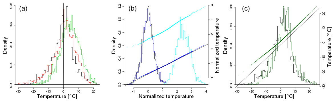
Figure 2 (a) Histograms of initial (black) reanalysis data (Dee et al., 2014) from 1979–2016 winter (DJF) from the location that includes Chicago. The initial LENS model data from the same period are shown in red. The final years, 2059–2096, of LENS model data are shown in green. (b) Normalized temperature distributions. The distribution of normalized reanalysis temperature is shown in black. The distribution after applying the shape transformation ${\stackrel{\mathrm{̃}}{G}}_{d,t_{\mathrm{f}}}^{-\mathrm{1}}\left({\stackrel{\mathrm{̃}}{G}}_{d,t_{\mathrm{p}}}\left(\stackrel{\mathrm{̃}}{X}\right(d,t_{\mathrm{p}}\left)\right)\right)$ is shown in dark blue. These values are shifted by $m_y(d,t_{\mathrm{f}})-m_y(d,t_{\mathrm{p}})$ and scaled by $\frac{r_y(d,t_{\mathrm{f}})}{r_y(d,t_{\mathrm{p}})}$ (light blue). (c) The initial normalization to the reanalysis is undone, yielding a distribution for the transformed observations (dark green) and are compared to the untransformed reanalysis (black). Panels (b) and (c) also show qq-plots on the right y axis to make it easier to see changes in the tails of the distributions.

Our procedure for carrying out this transformation is novel in several ways. First, for any given day of the year, it naturally allows a separate transformation from any one year during which both model output and observations are available to any year in which model output is available. Second, it separately accounts for linear transformations in both the observations and model output, with the consequence that if the results from the model output only show linear transformations in temperature between the present and the future, then the transformation applied to the observations will also be linear. Third, it transforms even highly extreme observations in a natural way without making strong assumptions about the tails of temperature distributions.

Although outside the scope of this paper, our technique can be modified to swap the assumptions in Eq. (2) with the assumption that the discrepancy between model and observations is time-independent, as would be the case in a bias correction approach. That is, following Li et al. (2010) for example, we would replace the assumption of Eq. (2) with ${\stackrel{\mathrm{̃}}{F}}_{d,t_{\mathrm{p}}}^{-\mathrm{1}}\left({\stackrel{\mathrm{̃}}{G}}_{d,t_{\mathrm{p}}}(\cdot )\right)={\stackrel{\mathrm{̃}}{F}}_{d,t_{\mathrm{f}}}^{-\mathrm{1}}\left({\stackrel{\mathrm{̃}}{G}}_{d,t_{\mathrm{f}}}(\cdot )\right).$ The transformation recommended by Li et al. (2010) is, leaving out normalization,

$$\begin{array}{ll}{\displaystyle }\widehat{X}(d,t_{\mathrm{f}})& {\displaystyle }=Y(d,t_{\mathrm{f}})+F_{d,t_{\mathrm{p}}}^{-\mathrm{1}}\left(G_{d,t_{\mathrm{f}}}\right(Y(d,t_{\mathrm{f}}))\\ \text{(4)}& {\displaystyle }& {\displaystyle }-G_{d,t_{\mathrm{p}}}^{-\mathrm{1}}\left(G_{d,t_{\mathrm{f}}}\left(Y\right(d,t_{\mathrm{f}}\left)\right)\right)).\end{array}$$

The fundamental difference in these two approaches is that in Eq. (3), we modify model output instead of projecting observations as is done in Eq. (2). When a large ensemble of model output is available, a drawback of Eq. (3) is the need to estimate the observational CDF F, which has fewer data to support its estimation. Nevertheless, both techniques Eqs. (2) and (3) allow for a smooth seasonal trend fitted on all data simultaneously. As discussed in Leeds et al. (2015), another important difference between these two approaches is that Eq. (2) retains characteristics of spatial and temporal dependence in the observations, whereas Eq. (3) assumes model output captures these dependencies appropriately. Leeds et al. (2015) and Poppick et al. (2017) describe methods for transforming observed daily temperature time series that allows for changes in means, variances, and temporal correlations in the future, but does not consider changes in the shapes of distributions. We discuss the possibility of combining this approach with the methods described here to allow for changes in both marginal distributions and temporal dependence of daily temperatures in Sect. 5.

3.2 Estimating the quantiles

A large body of work has been dedicated to fitting quantiles (Koenker, 2005), mostly from a frequentist perspective (Koenker, 2004; McKinnon et al., 2016; Rhines et al., 2017), although there is a Bayesian literature for quantile regression (Yu and Moyeed, 2001; Reich et al., 2011; Kozumi and Kobayashi, 2011; Geraci and Bottai, 2014). We are particularly interested in fitting quantiles while imposing a smoothness constraint on the estimates (Koenker and Schorfheide, 1994; Yu and Jones, 1998; Oh et al., 2011; Reiss and Huang, 2012).

The methods for estimating quantiles used here expand on the approach used in Haugen et al. (2018), where a fixed set of spline functions were used as a basis for fitting each quantile, similar to Wei et al. (2006). The main novelty over Haugen et al. (2018) is to estimate more extreme quantiles as exceedances beyond less extreme quantiles. The idea of using estimates at less extreme quantiles to constrain estimates at more extreme quantiles also appears in Liu and Wu (2009), with the added constraint that estimated quantiles should not cross. Subject to this non-crossing constraint, Liu and Wu (2009) use the same set of regressors for all quantiles, whereas we reduce the number of regressors for estimating exceedances beyond certain quantiles. Due to the large number of observations available (180 years and 50 simulations), the quantiles are fairly well estimated for the number of spline functions used and we did not have any problems with estimated quantiles crossing. Nevertheless, especially when estimating a large number of quantiles, methods that guarantee no crossings may be advisable. For a more in-depth discussion of quantiles crossing, see for example Bondell et al. (2010) and references therein.

We model the CDF of temperature by assuming each quantile is smoothly varying in both temporal dimensions, day of the year $d\in [\mathrm{1},\mathrm{365}]$ (there is no leap year in the CESM), and year $t\in [\mathrm{1920},\mathrm{2099}]$, using splines of different complexity as predictors of the quantiles. The seasonal basis functions are constrained to periodic splines, while the long-term basis functions are constrained to natural splines (Friedman et al., 2001). We also include historical zonal volcanic forcings as a regressor, Z_volc (Sriver et al., 2015). For quantiles between 0.1 and 0.9, we largely follow the approach taken in Haugen et al. (2018). Specifically, we find that seasonal effects for quantiles between 0.1 and 0.9 are well described by a periodic spline with 14 degrees of freedom, and long-term yearly effects are modeled by a natural spline with 6 degrees of freedom. We include interaction terms between seasonal and long-term effects to allow seasonal patterns to change slowly over time, but only use 3 seasonal basis functions with the same 6 long-term basis functions resulting in $\mathrm{6}\times \mathrm{3}=\mathrm{18}$ degrees of freedom to capture this effect.

Write $Z=[Z_{\mathrm{1}},Z_{\mathrm{2}},\mathrm{\dots },Z_k,Z_{\mathrm{volc}}]$ for the matrix whose columns are the values for these spline basis functions for each day and year. Each row of Z corresponds to a day of the year, d, and a year, t, and is denoted $Z(d,t)\in {\mathbb{R}}^{k+\mathrm{1}}$. If we denote each temperature observation as X(d,t), then quantiles are estimated by $Z{\widehat{\mathit{\beta }}}_p$ at the pth percentile where β_p is obtained by solving the following optimization problem (Koenker and Bassett, 1978),

$$\begin{array}{ll}{\displaystyle }{\widehat{\mathit{\beta }}}_p& {\displaystyle }=\underset{\mathit{\beta }}{\text{min}}\left\{\sum _{d,t:X(d,t)\ge Z(d,t)\mathit{\beta }}p\left|X\right(d,t)-Z(d,t\left)\mathit{\beta }\right|\right.\\ \text{(5)}& {\displaystyle }& {\displaystyle }+\left.\sum _{d,t:X(d,t)<Z(d,t)\mathit{\beta }}(\mathrm{1}-p)\left|X\right(d,t)-Z(d,t\left)\mathit{\beta }\right|\right\}.\end{array}$$

When we are fitting quantiles to model output, the sum in Eq. (3) should be understood as summing over all simulations as well as all years and days. It is possible to use more formal methods to select the complexity of the model, as in Koenker and Schorfheide (1994), Oh et al. (2011), Daouia et al. (2013), and Fasiolo et al. (2017) for example. However, the basis functions we have chosen allow considerable flexibility in the evolution of seasonally varying quantiles, with the resulting estimates having quite small variances (see Sect. 4.1), so there may not be much to be gained by trying to optimize the selection of the number of basis functions. All computations are performed in R (R Core Team, 2013) and the quantile regressions are done with the package quantreg (Koenker, 2017).

We are particularly interested in estimating fairly extreme quantiles. The further out in the tail of the distribution one goes, the less effective information there is in the data about the corresponding quantile. Thus, we choose to use simpler models for exceedances beyond two well-estimated quantiles, here the 0.1 and 0.9 quantiles. Specifically, after first using a set of predictors to normalize the data, we fit another set of coefficients on the normalized data with the same predictors for quantiles between the 0.1 and 0.9 quantiles inclusive. Next, we fit more extreme quantiles of the distribution as exceedances outside the 0.1 and 0.9 quantiles, using a similar model but with fewer basis functions: a 3 degree of freedom seasonal spline and a linear time trend without interaction between these two dimensions. The effect of modeling the tails as exceedances is that the bulk trend is added on top of the tail trend and thus we retain a high level of detail in the tails in spite of the relatively lower degrees of freedom in the predictors. The tail quantiles estimated in this way are 0.001, 0.010, 0.025, 0.050, and 0.075 and 1 minus each of these values.

When projecting the observations, we consider the time-window 1979–2016, which we project 80 years into the future (years 2059–2096). As previously mentioned, we do not require a detailed modeling of the CDF of the observations, merely an estimate of the location and scale as a function of the two temporal dimensions. Because of the reduced time span of these observations we use fewer degrees of freedom in the splines, namely 10 seasonal and 1 temporal (i.e., linear) without any interaction terms. This normalization step is only included to put the observations and model output on the same scale, so it is not essential that the model used to normalize the observations captures finer details of the median and scale functions.

As already noted, we include zonal volcanic forcings in the statistical model as they are included in the CESM climate model for the historical period and cause substantial short-term changes in temperature. We also tried including the CO₂ forcings in our model, but they did not improve the predictions when used in addition to the spline in the yearly parameter, t, and were thus not included in our final model.

3.3 Uncertainty quantification

The availability of a large ensemble makes it possible to quantify the uncertainty of our estimates based on treating the n different ensemble members as independent and identically distributed realizations of the same stochastic process and thus avoid any modeling of dependencies within a single realization. Castruccio and Stein (2013) and Haugen et al. (2018), among others, have similarly exploited this assumption to produce uncertainty estimates based on climate model output using bootstrap procedures. Here, we choose to use jackknife estimates of bias and variance (Davison and Hinkley, 1997), another standard resampling approach that only requires re-estimating the model as many times as the number of ensemble members. Specifically, holding out each simulation in the ensemble one at a time and calculating a quantile map with the remaining simulations yield n=40 different quantile maps for the LENS ensemble from which the jackknife bias and variance are estimated. For each held-out simulation j we calculate an “influence function,” $l_{\mathrm{jack},j}=(n-\mathrm{1})(T-T_{-j})$, where T and T_−j are in our case the projected temperature quantiles with all simulations and with one simulation held out, respectively. Then, the jackknife estimate of variance is given by

$$\begin{array}{}\text{(6)}& v_{\mathrm{jack}}={\displaystyle \frac{\mathrm{1}}{n(n-\mathrm{1})}}\left(\sum l_{\mathrm{jack},j}^{\mathrm{2}}-n{b}_{\mathrm{jack}}^{\mathrm{2}}\right),\end{array}$$

where $b_{\mathrm{jack}}=-{\sum }_{j=\mathrm{1}}^n{l}_{\mathrm{jack},j}$ is the jackknife estimate of bias (Davison and Hinkley, 1997). As we will see in Sect. 4.1, the jackknife standard errors are quite small and, in particular, are generally much smaller than the noteworthy differences between the estimated transformations based on the two different ensembles. Thus, we will not generally report these standard errors, since they are likely a smaller source of uncertainty than unknown model biases. Nevertheless, the jackknife is a promising technique to assess the uncertainty of the projection due to the simulation variability. Although it is not obvious from Fig. 3, the jackknife estimate of variance scales inversely with the ensemble size, $v_{\mathrm{jack}}=O(\mathrm{1}/n)$ (Efron, 1981).

3.4 Evaluating the procedure using the perfect model approach

There is, of course, no direct way to evaluate the accuracy of a future climate projection using currently available data. However, if we are willing to assume that the discrepancies in the statistical characteristics of some quantity of interest between two models are comparable to the discrepancies between the output from some model and reality, then we can at least get a qualitative idea as to how well the procedure is working. Perhaps more realistically, we may be able to obtain something like a lower bound on the actual errors in the statistical characteristics of our climate projections. Specifically, by treating the output from a second model as pseudo-observations, we can apply our transformation method and then directly compare the statistical characteristics of these transformed pseudo-observations to the available future model output from this second model. This basic idea has been used frequently for evaluating statistical downscaling procedures, where it is called the perfect model approach (Dixon et al., 2016), but it is equally appropriate in the present setting of projecting observations into the future.

There are a number of ways one could summarize the results of such an analysis. One method is to fix a particular quantile, q, and apply the transformation from year t_p=1920 to some future year t_f for each day of the year. Both quantile maps are then plotted as a function of t_f and day of the year and differences between the two quantile maps can be taken for a succinct comparison, viz.

$$\begin{array}{}\text{(7)}& \left({\widehat{G}}_{d,t_{\mathrm{p}}}^{\mathrm{L}}{)}^{-\mathrm{1}}{\widehat{G}}_{d,t_{\mathrm{f}}}^{\mathrm{L}}\right(q)-({\widehat{G}}_{d,t_{\mathrm{f}}}^{\mathrm{S}}{)}^{-\mathrm{1}}{\widehat{G}}_{d,t_{\mathrm{p}}}^{\mathrm{S}}\left(q\right),\end{array}$$

where the superscript L refers to estimates based on the LENS ensemble and S to the SFK15 ensemble. Another approach is to first apply a projection based on one of the models forward in time and then apply the second model's projection backwards in time to the original time point. To be explicit, we perform the following operation,

$$\begin{array}{}\text{(8)}& \left({\widehat{G}}_{d,t_{\mathrm{p}}}^{\mathrm{S}}{)}^{-\mathrm{1}}{\widehat{G}}_{d,t_{\mathrm{f}}}^{\mathrm{S}}\right({\widehat{G}}_{d,t_{\mathrm{f}}}^{\mathrm{L}}{)}^{-\mathrm{1}}{\widehat{G}}_{d,t_{\mathrm{p}}}^{\mathrm{L}}\left(q\right).\end{array}$$

If there is a close correspondence between the models, this double quantile map will be close to the identity map for all days and years.

4 Results

4.1 Quantile maps for eight cities

We report here results for eight cities in the United States representing a broad range of geographical settings, where we build a detailed statistical model using both the LENS and the SFK15 ensembles. These statistical models define quantile maps that we use to project present observational data into the future. We see in Fig. 1 that LENS and SFK15 ensembles differ both from each other and from observations, but those present-day biases do not mean that the projected future changes for the two ensembles will necessarily be very different. The statistical model helps to illuminate evolving differences between the two ensembles. As a preliminary illustration, we show in Fig. 3 a simple median quantile fit of ensemble output at an example grid cell containing Seattle in historical and future years. The magnitude of the differences between the median fits is substantial, with LENS being warmer in all seasons other than winter. Temperature differences grow in the future projection, suggesting a greater warming in the LENS ensemble. Since both ensembles use the same forcing scenario, the discrepancy between the future temperatures could be attributed to the different model resolutions used in the two ensembles (∼1^∘ vs. ∼3.75^∘). For example, different resolutions capture the land–sea contrast and land topography differently.

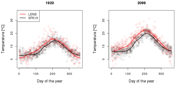
Figure 3 Example of quantile estimates fit to ensemble data, using daily mean temperatures in the years 1920 and 2099, at a grid cell containing Seattle, from LENS (red) and SFK15 (black). Solid lines are median quantile fits as a function of day of the year. Dots are ensemble output; for clarity we show only 3 % of all data, sampled randomly.

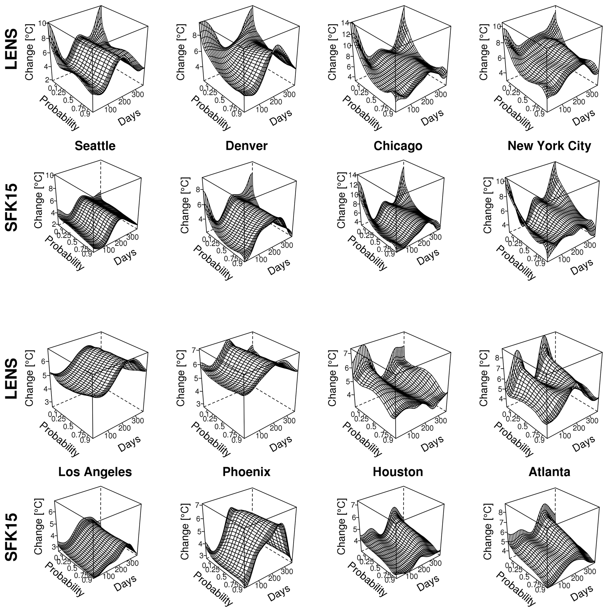
Figure 4 Quantile maps of temperature changes between 1989 and 2099 for multiple cities extracted from the SFK15 ensemble on the first and third rows and the LENS ensemble on the second and fourth rows. Temperature change is shown as a function of seasonality (days of the year) and non-exceedance probability of the temperature estimate. Note that z axes are consistent for each location but differ between locations.

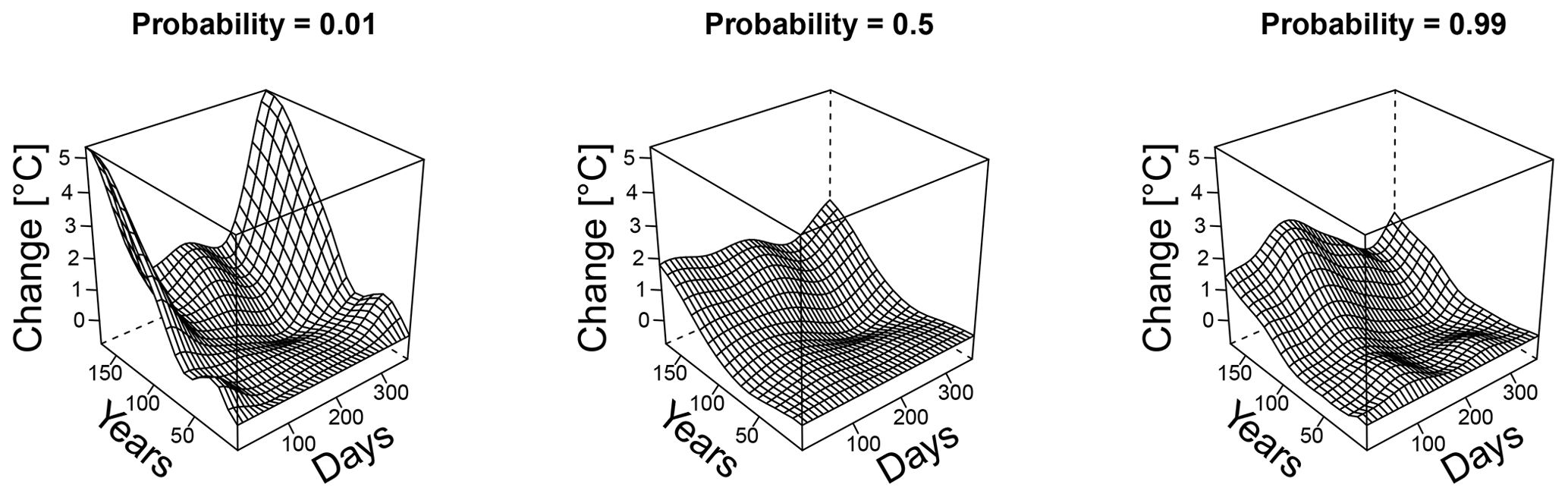
Figure 5 Differences between the two quantile maps (LENS minus SFK15) near Seattle as a function of years elapsed since 1920 and day of the year. At year zero, the quantile maps both produce zero change since the initial and final time are the same. As the years increase, so does the discrepancy between the two projections. Each panel shows these temperature discrepancies for a given non-exceedance probability of the temperature estimate. A positive change indicates a larger value for LENS than for the SFK15 ensemble. Notice the complex patterns both in long-term and seasonal effects, justifying the need for a model that fits all seasons simultaneously.

For both ensembles, we estimate a quantile map as a function of day of the year and long-term time for each of the eight locations using the methods in Sect. 3. For visualization purposes we choose to show the temperature quantile shift for quantiles between 0.001 and 0.999 from 1989 to 2099 as a function of day of the year, as seen in Fig. 4. This figure captures the nuances and complexities of the local temperature distributions. Notice the gradual yet distinct change from season to season. In the tails there is sometimes a large divergence of the temperature shift, particularly for Chicago in the winter, which shows the complexities in how quantiles change over time and the necessity of a detailed statistical model. Each location has unique features, but there are nontrivial differences between the two ensembles' quantile maps for all eight locations. Maybe the most important difference is the increased overall warming of the LENS compared to the SFK15 ensemble. Both ensembles show larger warming in the winter in the northern cities with the exception of Seattle. Thus, for at least Denver, Chicago and New York City, either ensemble will yield transformations that will especially increase the coldest wintertime temperature values.

We next examine the evolution in time of quantiles implied by these quantile surfaces. Consider, for each day of the year, the difference between a given quantile in 1920 and the same quantile for every year 1920+t for $t=\mathrm{0},\mathrm{\dots },\mathrm{180}$. Note this difference is necessarily 0 for t=0. As expected, all quantiles monotonically warm in t for all seasons and for both ensembles (Fig. A1). Of perhaps greater interest is the difference between these two transformations, using Eq. (4) and plotted in Fig. 5. We see that the LENS ensemble mostly shows increasingly greater warming than SFK15 as t increases, with differences of up to 5 ^∘C for non-exceedance probability 0.01 during the winter; see for example Maraun (2013) for related discussion.

Another way to assess how well the transformation approach might work in practice is the double transformation given by Fig. (5). We see significant seasonally dependent discrepancies between the two projection models derived from the LENS and the SFK15 ensemble (Fig. 6). The more prominent discrepancies are many times larger than the standard errors for the LENS transformation (Fig. 7) given by the jackknife procedure described in Sect. 3.3 and, therefore, would be statistically significant by any reasonable measure. Thus, to avoid obscuring the figures, we do not display statistical uncertainties in our figures for quantile maps.

To show explicitly how our procedure benefits from the large ensemble, we split up the 40-run LENS ensemble into 8 ensembles of size 5 and estimate the transformation for each of them. Variations between these mini-ensemble temperature projections are on the order of 1 ^∘C as shown in Fig. 8 where we show, relative to the results for the full 40-simulation ensemble, 8 individual quantile maps using 5 LENS simulations each for Chicago. There is some notable variability in the mini-ensemble results. For example, quantile maps 1 and 6 show substantial differences from each other and from the full ensemble results, especially at more extreme quantiles. Nevertheless, comparing to the quantile map for the full ensemble in Fig. 4, these variations are small enough that the results from a 5-member ensemble are still informative about some aspects of the seasonally varying quantile transformation.

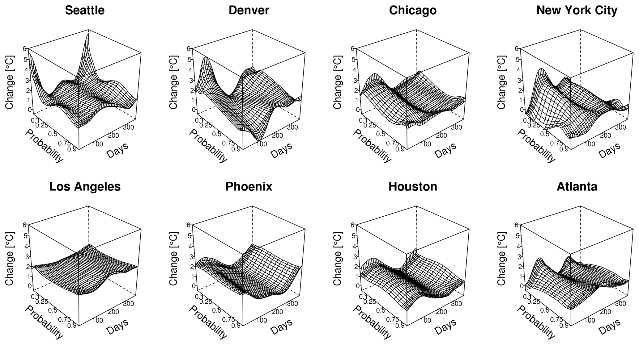
Figure 6 A double quantile map calculated for eight locations, first applying the map estimated from the LENS ensemble from year 1990 to 2090 followed by the inverse map estimated from the SFK15 ensemble from 2090 to 1990. Each map shows only the difference between the mapping and the original temperature. Positive values indicate that the LENS ensemble will transform to warmer temperatures in the future than SFK15 does. If the LENS and the SFK15 quantile maps were the same, these changes would be identically zero.

Figure 7 Standard deviation of the temperature change from 1990 to 2090, using a jackknife estimate on the 40 simulations (see Fig. 3). The error is approximately an order of magnitude smaller than the larger discrepancies between the LENS and the SFK15 quantile maps (see Figs. 5 and 6). Thus, these larger discrepancies are strongly statistically significant by any reasonable measure.

Figure 8 For 8 sets of 5 mutually exclusive simulations, panels show differences between quantile map estimates based on 5 simulations and the quantile map estimate using the full LENS 40-simulation ensemble (see Fig. 4) for Chicago.

4.2 Perfect model approach

We next employ the perfect model approach described in Sect. 3.4. Specifically, using the model built from SFK15 ensemble for the whole simulation period 1920–2100, we treat the portion of the LENS ensemble from 1979–2016 as our pseudo-observational data and project this forward in time by 80 years and compare with the LENS data during this future time, namely 2059–2096. Each of the 40 LENS simulations are treated as independent pseudo-observational data and are normalized individually using 10 seasonal and 1 temporal degree(s) of freedom, without interaction terms. Using this normalization and the quantile map from the SFK15 ensemble, the LENS data from 1979–2016 are transformed using Eq. (2). For comparison, we also give results applying the quantile map estimated from the full LENS ensemble to a single LENS run treated as pseudo-data, which should work very well since we are testing the LENS model on itself.

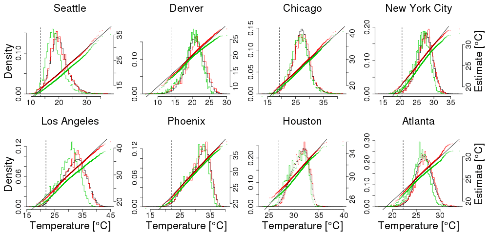
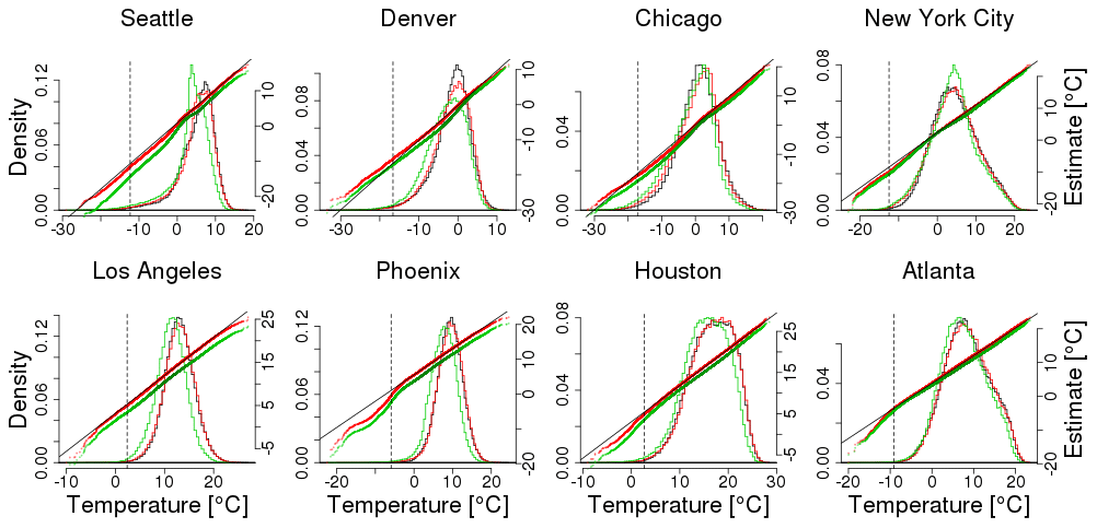
An example comparison between the two models is shown in Fig. 9, where we show winter temperature projections near Seattle with histograms and qq-plots. Figure 10 compares projections for all eight locations (see Fig. A2 for summertime results); it is clear that simulating data from the same ensemble as used in building the quantile map yields much better agreement than using a quantile map from the other ensemble. This difference was already foreshadowed when we compared the quantile maps in Fig. 4. The difference is not a function of the particular ensemble member chosen. Since the LENS ensemble includes 40 simulations, we can apply this perfect model test to all 40 of them, yielding a much larger sample of projections. Resulting histograms and qq-plots are smoother, but look very similar to Fig. 8 (Fig. A3). One might suspect that the difference between ensembles stems from their different resolutions. While resolution may play some role, a simple upscaling of the LENS data to match the SFK15 data does not ameliorate this discrepancy (results not shown).

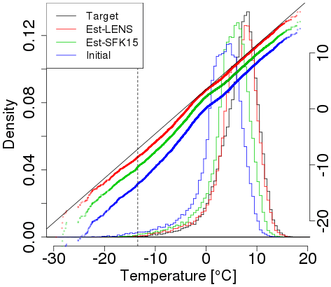
Figure 9 Comparisons between actual and projected LENS data for winter (DJF) using a model fit from the LENS data (red) and using a model fit from the SFK15 ensemble (green) near Seattle. The projected data are obtained by using 40 simulations of the time period 1979–2016 (viz. “Initial” shown in blue) projected 80 years into the future, 2059–2096. Both projection estimates are compared against the actual LENS model output during the same period, 2059–2096 (viz. “Target” shown in black). Corresponding qq-plots are juxtaposed using the same horizontal axis. The dashed vertical line represents the .01 quantile in the initial observations. LENS estimates are, not surprisingly, closer to the target than the SFK15 estimates since the LENS quantile map uses the LENS data while the SFK15 estimate does not involve the LENS data in building its quantile map.

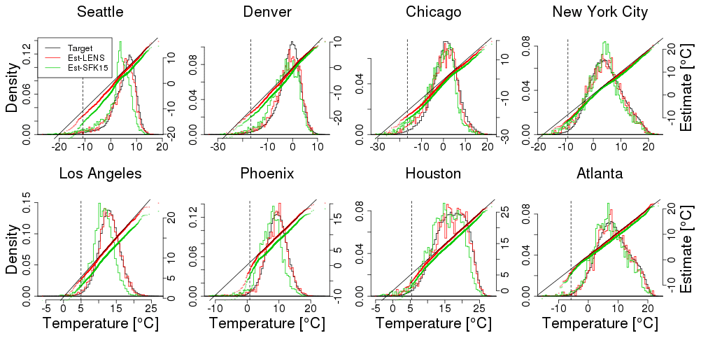
Figure 10 Similar to Fig. 9; comparisons between actual and projected LENS data for winter (DJF) using a model fit from the LENS data (in red) and using a model fit from the SFK15 ensemble (in green). Unlike Fig. 9, the projected data are obtained from one single simulation of the time period 1979–2016 projected 80 years into the future, 2059–2096. The actual target data draw from all 40 simulations (shown in black). The dashed vertical line represents the .01 quantile of the initial distribution.

4.3 Multi-fidelity modeling

In the present setting we have roughly equal numbers of runs for both resolutions of CESM. In many instances, one might have many more runs at lower resolution because of the lower cost of those runs. This situation bears some resemblance to what is known as multi-fidelity surrogate modeling in the computer modeling literature; see for example Kennedy and O'Hagan (2000), Forrester et al. (2007), Le Gratiet and Garnier (2014), and He et al. (2017). The goal in these works is generally to predict the value of some fairly low-dimensional result of some process, perhaps even univariate, as a function of some input parameters, by using a well-chosen combination of observations, a small number of high-fidelity computer model simulations and a larger number of lower-fidelity simulations. In the present work, we are focusing on a single scenario of forcings, so that the problem of interpolating in parameter space is not addressed here. The present situation's difficulty is caused by the highly multivariate and stochastic nature of the process we seek to simulate (the space–time climate system) and that we are most interested in the simulation for a setting for which we have no observational data (a future with much higher CO₂ concentrations than exists in the historical record). There could be scope for developing analogs for the types of methods first introduced in Kennedy and O'Hagan (2000) that assume that the computer models of various fidelity and the observed process can be modeled as jointly Gaussian processes that depend on the input parameters of interest, but here we just consider a very simple method for combining the full ensemble of SFK15 simulations with a single run of the LENS ensemble as a tool for estimating the quantile transformations we need to simulate future climate.

To fit the SFK15 quantile map followed by a LENS re-calibration, we first use the detailed statistical model (or quantile map) applied in previous sections to the 50 SFK15 simulations, so including an intercept, 14 seasonal terms, 6 long-term temporal terms, 18 interaction terms, and a volcanic forcing term. We then reduce these 40 predictors to 4 components: component 1, an intercept; component 2, temporal (including the volcanic term); component 3, seasonal; and component 4, interactions. Specifically, using the notation from Sect. 3.2 and S(j) as the set of indices for each of the four components,

$$\begin{array}{}\text{(9)}& W_j(d,t)=\sum _{i\in S\left(j\right)}{Z}_i(d,t){\widehat{\mathit{\beta }}}_i,j=\mathrm{1},\mathrm{\dots },\mathrm{4},\end{array}$$

where ${\widehat{\mathit{\beta }}}_i$ represents the fitted coefficient of basis function Z_i from the original quantile map using the full SFK15 ensemble. Thus, ${\sum }_{j=\mathrm{1}}^{\mathrm{4}}{W}_j(d,t)$ is the quantile map for day d and time t based on the SFK15 ensemble. We recalibrate this quantile estimate using an estimate of the form ${\mathit{\gamma }}_{\mathrm{1}}{W}_{\mathrm{1}}(d,t)+{\mathit{\gamma }}_{\mathrm{2}}{W}_{\mathrm{2}}(d,t)+W_{\mathrm{3}}(d,t)+W_{\mathrm{4}}(d,t)$, estimating γ₁ and γ₂ using quantile regression applied to a single LENS run. That is, only the temporal and the intercept components are re-estimated for each quantile simulation using Eq. (3); the seasonal and the interaction terms are kept at their estimated values from the SFK15 fit. Other choices are certainly possible here, but even this simple procedure is sufficient to show the benefit of this type of re-calibration.

Using this quantile map, we can then project observations into the future using the procedure described in Sect. 3. For Seattle, we projected each year of reanalysis data into the single future year 2099 based on the full SFK15 ensemble, the full LENS ensemble and the full SKF15 ensemble re-calibrated using one LENS simulation. We chose winter in Seattle because estimated shape transformations for SFK15 and LENS showed large differences for this location and season and so should provide a difficult challenge for our approach. Nevertheless, the results, shown in Fig. 11, demonstrate that we can largely correct for the differences between the projections based on the full SFK15 and LENS ensembles by using just one LENS simulation in addition to the full SFK15 ensemble, although we can see that the coldest temperature values are not warmed sufficiently. The method should work even better for Seattle summers or any time of year for Phoenix.

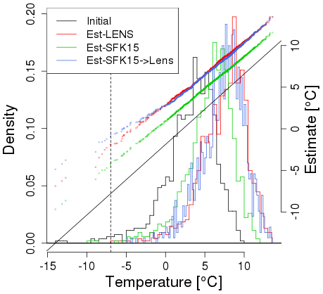
Figure 11 Comparisons between reanalysis data from the winter months (DJF) in Seattle in the period 1979–2016 projected with three different methods. (1) Using the 40-member LENS ensemble to construct a quantile map (shown in red), (2) using the 50 simulations from SFK15 (in green), and (3) using method (2) and then re-calibrating the quantile map using one LENS simulation (in blue). For all three models, every year is projected into year 2099 and compared using qq-plots juxtaposed by histograms. We project into a single year here instead of projecting each year by a constant time shift to show the flexibility of the method. The fact that the re-calibrated method (in blue) is close to the LENS model shows that even one high-resolution simulation can get close to the results based on all 40 LENS simulations when aided by a set of low-resolution simulations (SKF15). The dashed vertical line in each plot represent the .01 quantile for the initial distribution.

5 Discussion and conclusions

Taking advantage of two large ensembles of climate model output, we project observations into the future based on their seasonality and long-term time evolution from 1920 to 2099. By projecting the whole observational record simultaneously, temporal and spatial dependencies in the observational record that a climate model may not accurately capture are maintained in the future projections. Our method, building on the quantile regression approach in Haugen et al. (2018), differs from other methods by computing quantile maps simultaneously for all data available in the ensemble, instead of using a window of nearby data or separating data by season or month. Using two temporal dimensions in the statistical model for the quantile map yields insight into the way temperature transitions across seasons. While this technique is primarily focused toward projecting current observations into the future, it could be adapted to bias-correct future model output (see for example Li et al., 2010).

The ensemble of simulations makes it possible to estimate the uncertainty of the quantile projections based on the jackknife variance, which shows that the simulation standard deviation is approximately one order of magnitude lower than the larger model discrepancies as seen when comparing projections between the LENS and the SFK15 ensemble. Thus, efforts to realistically assess the full uncertainty in estimated transformations based on large ensembles should focus on the impact of model biases on these estimates.

To assess how well our method works, we use two ensembles, one treated as pseudo-observations and the other to build our quantile map. Since the LENS data have marginal distributions that resemble the ERA-Interim data more closely (Fig. 1), this ensemble is treated as pseudo-observations. We see substantial and statistically significant differences between the two ensembles, where the higher-resolution ensemble shows greater warming, especially at lower quantiles in some locations.

The nested statistical model and the large ensemble used in building the quantile map enable stable estimates of quantiles in the extreme tails, e.g., the 0.001 and the 0.999 quantiles. When nesting models, we first estimate the 0.1 and the 0.9 quantiles and then consider only the exceedances beyond these quantiles to model any more extreme quantiles. These further quantiles are modeled with fewer degrees of freedom to match the fewer observations available beyond these thresholds, providing a more stable estimate. Extreme quantiles beyond the 0.999 quantile are all projected by the same amount as a function of seasonality, avoiding further parametrization using extreme value distributions.

Following Leeds et al. (2015) and Poppick et al. (2017), we advocate for the use of delta change approaches to future climate simulation when feasible. The goal in these works was to use model output to learn about changes in temporal means and covariances in daily temperature and then make transformations in the spectral domain to modify observational data to capture these changes in means and covariances. The transformations used were linear in the observations and, hence, did not address possible changes in the shapes of temperature distributions. As the present work shows, both CESM ensembles show clear changes in the shapes of daily temperature distributions. Thus, it would be of interest to develop a delta change method that could account for changes in both shapes and in covariances. One possibility would be to first employ the methods in Poppick et al. (2017) for transforming means and covariances in transient climates and then apply the methods developed here to change shapes of distributions.

Having estimated how every year in the observational record would be projected into any future year spanned by the climate model, we can produce projections spanning different numbers of years than the original observational record. For example, if we take the observational record to be of 40 years length, which is the approximate length of the post-satellite reanalysis era, we are not just restricted to simulating a single 40-year period but can for example instead produce four projections of the same future decade by separately projecting each of four 10-year periods in the observational record into that decade. Similarly we can project every observed year into one future year, e.g., 2099 (see Fig. 11). Same-year projections open up the possibility of quantifying the uncertainties in making projections for a given future year due to having a limited observational record by treating each of these projected years as an independent sample from the relevant distribution.

If it is expensive to run a high-quality or high-resolution model, an alternative we propose is to first build a quantile map using a less expensive model, then reduce the dimensionality of the prediction space and recalibrate the quantile map with the limited data from the expensive model by re-estimating the regression parameters in this lower-dimensional space. While the results show a clear improvement in the projections after the recalibration, there is clearly scope for further development using this approach.

In this work, we have only modeled marginal distributions of a single quantity, average daily temperature. The general methodology can be applied to other quantities, although some care would be needed in extending the approach to daily precipitation, which will generally have a large fraction of zeroes (Friederichs and Hense, 2007; Wang and Chen, 2014). A simple way to handle transformations of multiple variables is to apply individual univariate transformations to each variable separately. Since the transformations will be applied to observational data, the transformed data will largely retain the dependencies between the quantities that exist in the observations, in keeping with the principle of relying on the data rather than the model output to capture complex dependencies in the climate system. Note that this approach assumes these spatiotemporal dependencies do not change over time. Thus, if the climate model projects a credible change in this dependency structure, it would not be present in the projection (Zscheischler and Seneviratne, 2017). As an extension, one could consider an approach inspired by Bürger et al. (2011) and Cannon (2016) to match the multivariate correlation structure with the future (changed) correlation structure.

Appendix A

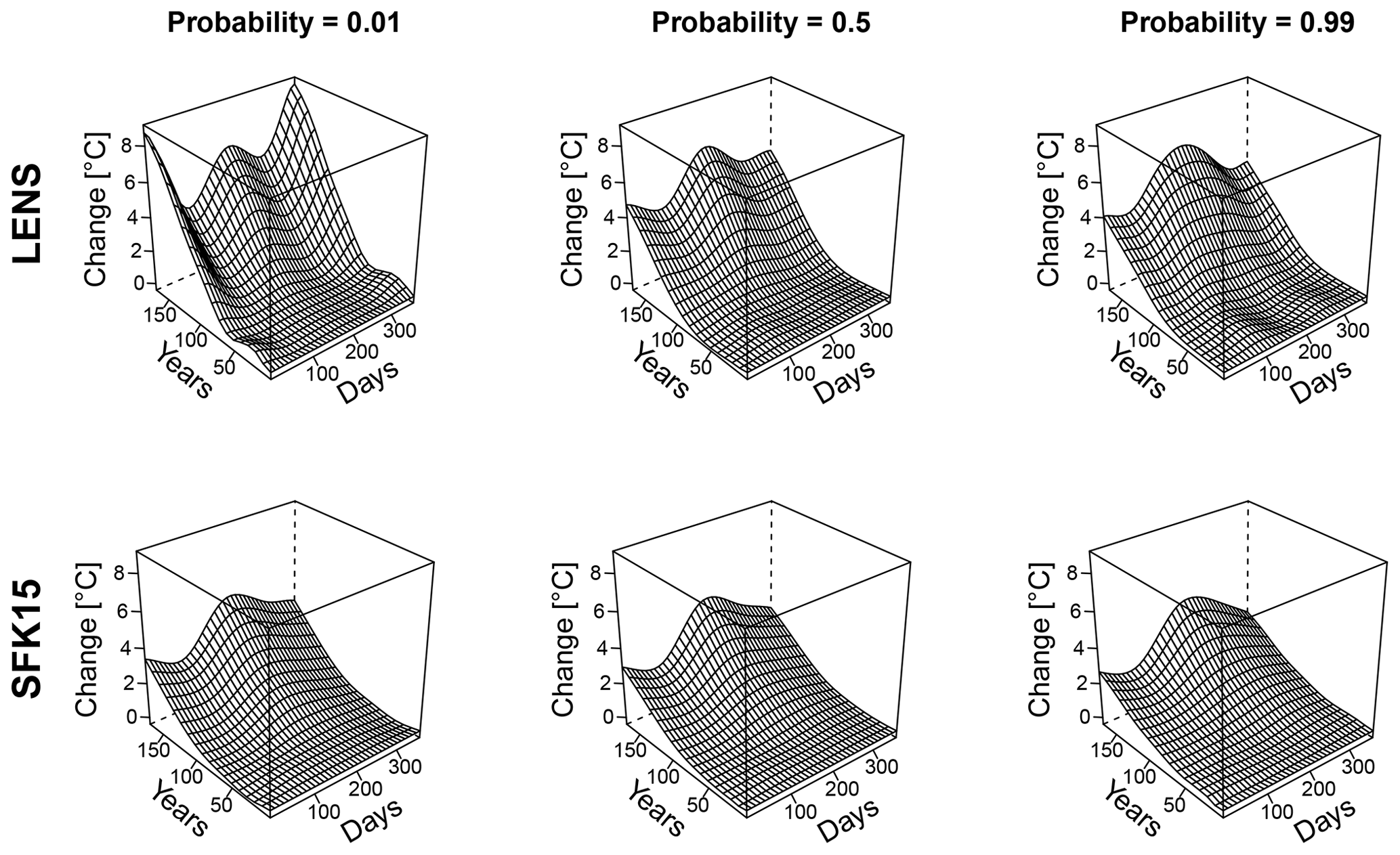
Figure A1 LENS and SFK15 quantile maps at a grid cell containing Seattle as a function of years elapsed since 1920 and day of the year. At year zero, the quantile maps both produce zero change since the initial and final time are the same. Each column of plots shows the changes in quantiles as a function of the non-exceedance probability given for that column.

Figure A2 Same as Fig. 10 but for the summer months June, July, and August (JJA).

Figure A3 As in Fig. 10, only now we show all 40 simulations combined instead of a single simulation from each ensemble. The comparisons are now less affected by random noise and some features stick out more clearly, e.g., in Seattle or the mean shift between the projections in Los Angeles.