Skewed logistic distribution for statistical temperature post-processing in mountainous areas

Nonhomogeneous post-processing is often used to improve the predictive performance of probabilistic ensemble forecasts. A common quantity used to develop, test, and demonstrate new methods is the near-surface air temperature, which is frequently assumed to follow a Gaussian response distribution. However, Gaussian regression models with only a few covariates are often not able to account for site-specific local features leading to uncalibrated forecasts and skewed residuals. This residual skewness remains even if many covariates are incorporated. Therefore, a simple refinement of the classical nonhomogeneous Gaussian regression model is proposed to overcome this problem by assuming a skewed response distribution to account for possible skewness. This study shows a comprehensive analysis of the performance of nonhomogeneous post-processing for the 2 m temperature for three different site types, comparing Gaussian, logistic, and skewed logistic response distributions. The logistic and skewed logistic distributions show satisfying results, in particular for sharpness, but also in terms of the calibration of the probabilistic predictions.

1 Introduction

Probabilistic weather forecasts have become state-of-the-art in recent years (Gneiting and Katzfuss, 2014). As such, they are important for addressing the chaotic nature of the atmosphere and expressing the uncertainty of a specific forecast (Lorenz, 1963). The expected uncertainty is typically provided by an ensemble prediction system (EPS; Leith, 1974) where multiple forecasts are produced by a numerical weather prediction (NWP) model with slightly perturbed initial conditions, model physics, and parameterizations. However, it was found that these forecasts often show systematic errors in both the expectation and the uncertainty due to required simplified physical equations, insufficient resolution, and unresolved processes (Bauer et al., 2015).

Statistical post-processing techniques (Gneiting and Katzfuss, 2014), such as Gaussian ensemble dressing (GED; Roulston and Smith, 2003), nonhomogeneous Gaussian regression (NGR or EMOS; Gneiting et al., 2005), a nonhomogeneous mixture model approach with similarities to Bayesian model averaging (BMA; Raftery et al., 2005), or logistic regression (Wilks, 2009; Messner et al., 2014), are one possibility to correct for these errors. These methods have been extensively tested for air temperature forecasts and other quantities, with NGR (with various extensions) representing one of the most popular approaches.

The two most important properties of probabilistic forecasts are sharpness and calibration (Gneiting et al., 2007) which have to be considered jointly. Accurate forecasts should be as sharp as possible but not overconfident, as this would result in a loss of calibration. Previous studies show that extensions of the classical NGR method (Schefzik et al., 2013; Scheuerer and Büermann, 2014; Möller and Groß, 2016; Dabernig et al., 2017) and other temperature post-processing methods (Hagedorn et al., 2008; Verkade et al., 2013; Feldmann et al., 2015; Wilks, 2017) are able to improve the predictive performance of the classical NGR with respect to specific predictive performance measures such as sharpness and calibration.

However, in recent publications, the probability transform histograms (PIT; Dawid, 1984) presented often do not show the desired perfectly uniform distribution to confirm calibration (cf., Scheuerer and Büermann, 2014, Fig. 5c,g; Möller and Groß, 2016, Fig. 4c; or Messner et al., 2017, Fig. 7). More specifically, the histograms indicate skewness in the residual distribution. As a marginal Gaussian model without covariates can already exhibit skewness for temperature data (Toth and Szentimrey, 1990; Warwick and Curran, 1993; Harmel et al., 2002), skewness is supposed to vanish if covariates are incorporated. Nevertheless, the residual distribution is still found to be skewed even after adjustment using covariates (Messner et al., 2017). As covariates are based on the output of NWP models, a remaining skewness is likely to originate in small-scale or local atmospheric processes that are insufficiently or not at all resolved by the NWP models. Locations in regions where topography is only coarsely resolved in the model are an example of this. As a result, many thermally induced slope and valley wind systems as well as subsidence/lifting zones (Steinacker, 1984; Whiteman, 1990; Zängl, 2004) will be absent, which may cause residual skewness in the post-processed forecasts.

So far, most studies assume a Gaussian response distribution for their temperature post-processing methods (Gneiting et al., 2005; Hagedorn et al., 2008; Verkade et al., 2013; Scheuerer and Büermann, 2014; Möller and Groß, 2016; Gebetsberger et al., 2018; Dabernig et al., 2017). As the Gaussian distribution is symmetric, it is not able to account for possible skewness by itself. Hence, this article proposes an extension of the nonhomogeneous Gaussian regression framework (Gneiting et al., 2005) using a skewed rather than a symmetric response distribution in order to obtain sharp and calibrated probabilistic temperature forecasts. To examine the need for asymmetry, probabilistic temperature forecasts are presented for a set of stations with different characteristics including sites in the European Alps and plain areas across central Europe. Moreover, the current study uses a long-term data set for training the statistical models, and compares the results to the widely used sliding training period approach where a fixed number of past training days is used (Gneiting et al., 2005; Scheuerer and Büermann, 2014; Feldmann et al., 2015; Möller and Groß, 2016).

2 Methods and data

Section 2.1 briefly describes the regression framework followed by the response distributions as used in this study (Sect. 2.2). The data and statistical model specifications are introduced in Sect. 2.3, and the verification methodology to access the predictive performance is introduced in Sect. 2.4.

2.1 Nonhomogeneous regression framework

The nonhomogeneous Gaussian regression (NGR) framework as proposed by Gneiting et al. (2005) is a special case of a distributional regression model (Klein et al., 2015) and can be expressed in its general form as

$$\begin{array}{}\text{(1)}& y\sim \mathcal{D}\left(h_{\mathrm{1}}\left({\mathit{\theta }}_{\mathrm{1}}\right)={\mathit{\eta }}_{\mathrm{1}},\mathrm{\dots },h_K\left({\mathit{\theta }}_K\right)={\mathit{\eta }}_K\right).\end{array}$$

A response variable y is assumed to follow some probability distribution 𝒟 with distribution parameters θ_k, $k=\mathrm{1},\mathrm{\dots },K$. Each parameter is linked to an additive predictor η_k using a monotone link function h_k. In this article we use the identity-link h_k(η_k)=η_k for the location parameter and a log-link for scale and shape parameters to ensure positivity during optimization, as proposed in Gebetsberger et al. (2017). Each linear predictor can be expressed by a set of additive predictors which have the following form:

$$\begin{array}{}\text{(2)}& {\mathit{\eta }}_k={\mathit{\eta }}_k({\mathbf{x}}_p,{\mathit{\beta }}_k)=f_{\mathrm{1}k}({\mathit{x}}_{\mathrm{1}},{\mathit{\beta }}_{\mathrm{1}k})+\mathrm{\dots }+f_{Pk}({\mathit{x}}_P,{\mathit{\beta }}_{Pk}),\end{array}$$

including various (possibly nonlinear) functions f_pk, $p=\mathrm{1},\mathrm{\dots },P$. Hence, x_p defines a matrix of covariates used, and β_pk is the vector of the regression coefficients to be estimated.

Classical NGR (Gneiting et al., 2005) assumes the Gaussian response distribution, which is described by the two parameters for location and scale. In ensemble post-processing applications, it is common to use the ensemble covariate which describes the observed variable of interest, e.g., ensemble temperature is used for temperature observations. The term nonhomogeneous relates to the residual variance, which, in contrast to linear (homogenous) regression, varies depending on the covariate value used for the Gaussian scale parameter (Wilks, 2011). The optimization of the regression coefficients is originally carried out by minimizing the continuous ranked probability score (CRPS; Hersbach, 2000), although it can also be estimated by maximum likelihood estimation (ML; Aldrich, 1997). Both approaches are compared in Gebetsberger et al. (2018), where it is shown that CRPS optimization obtains sharper, but not necessarily better, calibrated probabilistic predictions than ML estimation.

2.2 Response distributions

This study compares three different distributions for temperature post-processing: (i) the frequently-used Gaussian distribution, (ii) the symmetric logistic distribution, and (iii) the generalized logistic distribution type I (Fig. 1). The logistic distribution is used to assess the impact of having slightly heavier tails (Gebetsberger et al., 2018). The generalized logistic distribution type I is of particular interest as it allows one to account for possible skewness in the data. For simplicity, it will be referred as the skewed logistic distribution in the following.

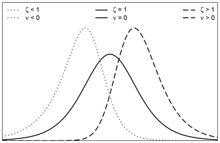
Figure 1 Density function of the skewed logistic distribution, illustrating the third moment (ν, skewness) depending on the chosen shape parameter ζ.

The skewed logistic distribution has the cumulative distribution function (CDF):

$$\begin{array}{}\text{(3)}& \mathrm{CDF}\left(x\right)={\displaystyle \frac{\mathrm{1}}{{\left(\mathrm{1}+\exp (-\frac{x-\mathit{\mu }}{\mathit{\sigma }})\right)}^{\mathit{\zeta }}}},\end{array}$$

with location parameter μ, scale parameter σ, and shape parameter ζ. The first derivation of Eq. (3) leads to the probability density function (PDF):

$$\begin{array}{}\text{(4)}& \mathrm{PDF}\left(x\right)={\displaystyle \frac{\mathit{\zeta }\cdot \exp \left(-\frac{x-\mathit{\mu }}{\mathit{\sigma }}\right)}{\mathit{\sigma }\cdot {\left(\mathrm{1}+\exp \left(-\frac{x-\mathit{\mu }}{\mathit{\sigma }}\right)\right)}^{\mathrm{2}\mathit{\zeta }}}}.\end{array}$$

The additional shape parameter ζ is responsible for the skewness. Figure 1 shows the PDF for three different shape parameter values of ζ and corresponding skewness ν. ζ is positive where values below 1 create negative skewness (heavier left tail, ν<0), whereas values above 1 produce positive skewness (heavier right tail, ν>0). For ζ≡1 the skewed logistic distribution describes the symmetric logistic distribution.

As an example, values for $\mathit{\zeta }=\mathit{\{}\mathrm{0.50},\mathrm{1},\mathrm{3.82}\mathit{\}}$ produce a skewness of $\mathit{\nu }=\mathit{\{}-\mathrm{0.85},\mathrm{0},\mathrm{0.85}\mathit{\}}$ as illustrated in Fig. 1. Details regarding the skewness calculation can be found in Appendix A.

2.3 Data and statistical models

2.3.1 Data

Results are presented at 27 different sites in central Europe (Fig. 2) for forecasts +12 to +96 h at 6-hourly intervals. The sites were selected to investigate the influence of different topographical environments. Therefore, the stations are subjectively clustered into three distinct groups representing Alpine sites located in inner-Alpine regions (12), foreland sites in the peripheral area close to the Alps (6), and plain sites in topographically flat areas (9). Nevertheless, statistical models described in the next subsection are estimated individually for each station and lead time, as each location and time of the day has its own site-specific characteristics.

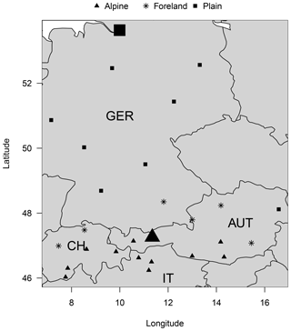
Figure 2 Study area and selected stations in Germany (GER), Switzerland (CH), Italy (IT), and Austria (AUT). The markers indicate stations classified as Alpine (triangle), foreland (star), and plain (square). Large symbols represent stations that are discussed in detail in this article: Innsbruck, Austria (large triangle), and Hamburg, Germany (large square).

Temperature observations are provided by automatic weather stations (10 min mean values). As input, 2 m temperature forecasts of the 50+1 member EPS of the European Centre for Medium-Range Weather Forecasts (ECMWF) are used. For this study only EPS forecasts initialized at 00:00 UTC are considered. The data set covers the time period from 1  January 2012 to 31 December 2015 resulting in 4 years of data that yield a sample size of approximately 1400 for each individual station and forecast lead time. The temperature covariate of the raw ECMWF ensemble is bilinearly interpolated to the individual sites.

In this article, detailed case studies will be shown for Innsbruck, Austria (Alpine site), and Hamburg, Germany (plain site; cf., Fig. 2), which differ – particularly with respect to their topographical environments. While the Alpine site is located in a narrow Alpine valley surrounded by high mountainous exceeding an altitude of 2500 m, the plain site is characterized by its proximity to the sea (100 km), its few hills, and an altitude below 160 m. Due to the necessary simplifications in the NWP model, the topography is missing large parts of the topographical structures, especially for the Alpine site (Stauffer et al., 2017, Figs. 1 and 3).

2.3.2 Statistical models

Similar to previous works (cf., Scheuerer and Büermann, 2014; Feldmann et al., 2015; Möller and Groß, 2016; Dabernig et al., 2017), we only utilize the ensemble mean ($\stackrel{\mathrm{‾}}{\mathrm{ens}}$) and ensemble standard deviation (SD_ens) of the 2 m temperature forecasts from the ECMWF EPS in this study. In the following model specification, the ensemble mean is used for the linear predictor of the location parameter μ, whereas the ensemble standard deviation is used for the linear predictor of the corresponding scale parameter σ.

While the Gaussian and the logistic distribution have only two parameters (μ and σ), the skewed logistic distribution has an additional shape parameter ζ. To be able to capture seasonality, a smooth cyclic spline f depending on the day of the year (DOY) is used in the linear predictor for all distribution parameters. The seasonal splines allow the regression coefficients to vary over the year, if needed, while the cyclic constraint avoids discontinuities at the turn of the year. As there is no obvious candidate among all of the parameters provided by the EPS, the shape parameter ζ of the skewed logistic distribution is solely expressed by a smooth cyclic spline. This allows the model to account for possible skewness in the residuals between the observed and forecasted 2 m temperature. The model specification for the study presented can be summarized as follows:

$$\begin{array}{}\text{(5)}& {\displaystyle }& {\displaystyle }y\sim \mathcal{D}(\mathit{\mu },\mathit{\sigma },\mathit{\zeta }),\text{(6)}& {\displaystyle }& {\displaystyle }\mathit{\mu }=f\left(\mathrm{DOY}\right)+{\mathit{\beta }}_{\mathrm{1}}\cdot \stackrel{\mathrm{‾}}{\mathrm{ens}},\text{(7)}& {\displaystyle }& {\displaystyle }\log \left(\mathit{\sigma }\right)=f\left(\mathrm{DOY}\right)+{\mathit{\gamma }}_{\mathrm{1}}\cdot \log \left({\mathrm{SD}}_{\mathrm{ens}}\right),\text{(8)}& {\displaystyle }& {\displaystyle }\log \left(\mathit{\zeta }\right)=f\left(\mathrm{DOY}\right),\end{array}$$

for which the additional parameter ζ is solely used for models utilizing the skewed logistic response distribution. The optimization of the regression coefficients for all parameters is performed employing likelihood based gradient boosting (R package “bamlss”; Umlauf et al., 2018). In this context gradient boosting is not used for variable selection, but to obtain regularized estimates for the regression coefficients. This is done by performing an additional 10-fold cross validation on the training data set to find the optimal stopping criterion based on the 10-fold out-of-sample root mean squared error. Table 1 shows a comprehensive overview of all of the models and the covariates used in the corresponding linear predictors.

Table 1 Covariates used in the linear predictors of the distributional parameters μ, σ, and ζ for all response distributions. $\stackrel{\mathrm{‾}}{\mathrm{ens}}$ and SD_ens represent the ensemble mean and the standard deviations of the ensemble 2 m temperature, respectively; f(DOY) represents the smooth cyclic seasonal effect.

2.4 Verification methodology

Different scores are used to assess the predictive performance of the models tested. The overall performance is evaluated by the logarithmic score (LS; Wilks, 2011) and the continuous ranked probability score (CRPS; Hersbach, 2000). The LS evaluates a forecast distribution by taking the logarithmic probability density value at the observed value, whereas the CRPS accounts for the whole forecast distribution.

Of particular interest for this study is the performance of the post-processing models in terms of sharpness and calibration (Gneiting et al., 2007). The sharpness of the probabilistic forecasts is verified using the average prediction interval width (PIW). Results for three different intervals are shown in this article: 50 %, 80 %, and 95 %. For example, the 80 % PIW describes the range between the 10th percentile and the 90th percentile of the probabilistic forecast. The smaller the PIW, the sharper the forecasts.

Calibration is visually evaluated using probability integral transform (PIT) histograms (Gneiting et al., 2007), which evaluate the forecasted cumulative distribution functions equivalent to the rank histogram (Anderson, 1996; Talagrand et al., 1997; Hamill and Colucci, 1998). In addition, the reliability index (RI; Delle Monache et al., 2006) and prediction interval coverage (PIC) are shown. The RI allows one to analyze an aggregated measure over a large number of individual PIT histograms. RIs are defined as ${\sum }_{i=\mathrm{1}}^I|{\mathit{\kappa }}_i-\frac{\mathrm{1}}{I}|$, where I defines the number of individual bins in a PIT histogram and κ_i defines the observed relative frequency in each bin. In this study we use a binning of 5 %. The RI describes the sum of the absolute deviation from each bin in a specific PIT histogram from perfect calibration. Thus, perfectly calibrated forecasts would show an RI of zero. PICs show the calibration for a specific interval. As for the PIW, PICs are shown for the 50 %, 80 %, and 95 % interval in addition to theoretical PICs of 50 %, 80 %, and 95 %. The closer the empirical PIC is to the theoretical PIC, the better the calibration.

3 Results and discussion

This section presents a detailed analysis of the different statistical models. Section 3.1 shows a detailed analysis of the long-term training window approach (see Sect. 2.3) for an Alpine valley site. These results are compared to the results for a plain site in Sect. 3.2. Section 3.3 shows a comprehensive analysis of the predictive performance of the proposed method for the three different groups of stations (Alpine, foreland, and plain sites), whereas Sect. 3.4 compares the proposed long-term training data approach against the frequently used sliding window approach.

All results presented in Sect. 3.1–3.2 are out-of-sample results using 4-fold block-wise cross-validation. For each model, station, and lead time, four individual regression models have been estimated using 3 years of data while one full year (2012, 2013, 2014, or 2015) is used as test data set. The comparison in Sect. 3.4 is based on out-of-sample results for the year 2015 if not stated otherwise. Sliding window models are estimated by minimum CRPS and maximum likelihood estimation as in Gebetsberger et al. (2018).

3.1 Alpine case study

Raw ensemble forecasts for Alpine sites cannot be directly used because the topography is not well resolved. Therefore, raw ensemble forecasts are typically characterized by small 80 % prediction interval widths (PIWs) around 3 ^∘C and large CRPS values around 4 (Stauffer et al., 2018). The large CRPS values are mainly driven by a systematic bias because of the difference between the real and model topography of the ECMWF. Additionally, the small PIW of the raw ensemble leads to underdispersive probabilistic predictions (Gebetsberger et al., 2018).

To show the performance of the proposed approach, the analysis for one selected site with a distinct Alpine character is shown (large triangle, Fig. 2). The left column of Fig. 3 presents the verification for this Alpine site. Figure 3 (top down) shows LS, CRPS, 80 % PIW, and RI for all forecast lead times. A dominant diurnal cycle for LS, CRPS, and the 80 % PIW can be seen for all three models, with the smallest (best) scores obtained during nighttime (00:00 and 06:00 UTC) and largest during daytime (12:00 and 18:00 UTC). The increased PIW during nighttime in combination with low RIs show that forecasts at night are sharper than during the day, although both are well calibrated. Overall, only a small decrease in the forecast performance can be identified with increasing lead time which implies comparable skill between the first and fourth forecast day.

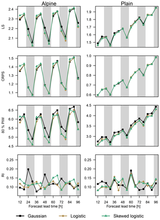
Figure 3 Performance measures at the selected Alpine site (left) and plain site (right) for all three models (Gaussian: squares; logistic: circles; skewed logistic: triangles). From the top down, the LS, CRPS, 80 % PIW, and RI are shown, and are evaluated for all forecasts +12 to +96 h ahead. Nighttime forecasts (00:00 and 06:00 UTC) are highlighted using vertical gray bars. Please note that the displayed range on the ordinate differs between the left and right column, except for RI.

When comparing the logistic model with the benchmark Gaussian model, the logistic model shows small improvements in LS, especially during nighttime. Similar behavior can be seen for the sharpness (80 % PIW) where the strongest improvements can be achieved during nighttime, but with an overall improvement for all lead times. Furthermore, the logistic model is able to remove large parts of the existing diurnal pattern in terms of calibration, showing a more homogeneous RI for all lead times time compared with the Gaussian model. The proposed skewed logistic model shows similar performance in all verification measures compared to the logistic model, with the largest improvements in sharpness during nighttime.

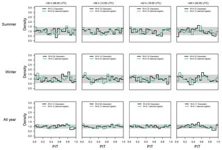
Figure 4 PIT histograms at the Alpine site for the Gaussian (black/dark line) and skewed logistic (green/bright line) models for the 2 d ahead forecasts (left to right: 06:00, 12:00, 18:00, and 00:00 UTC) corresponding to forecasts +30, +36, +42, and +48 h ahead. Top down, the PIT histograms are shown for summer only (June/July/August), winter only (December/January/February), and for the whole year. The gray horizontal bar shows the point-wise 95 % confidence interval around 1 which indicates perfect calibration.

Figure 4 shows PIT histograms for the 2 d ahead forecasts. To increase readability, only the Gaussian and skewed logistic models are shown. PITs are shown for 06:00, 12:00, 18:00, and 00:00 UTC to assess the characteristics for different times of the day. Top down PITs for the summer season, the winter season, and the full year are shown to highlight seasonal differences in calibration. Forecasts for day one, three, and four show a very similar picture (not shown).

Both, the Gaussian and logistic model, already show an almost uniform distribution, although for one particular hour of the day special features can be identified. The convex shape of the Gaussian model for the all year period at +48 h (bottom right) indicates overdispersion (peak at bin 0.5), while the asymmetry also indicates residual skewness (peak at bin 0.95). This is likely caused by the not yet resolved topography in the NWP. The overdispersion is more visible in the summer season for +48 h (Fig. 4, top right), where a peak can be seen at around 0.5, and two minima occur at 0.05 and 0.9, respectively. The skewed logistic distribution is able to produce a more uniform PIT which is also quantified by smaller RI values.

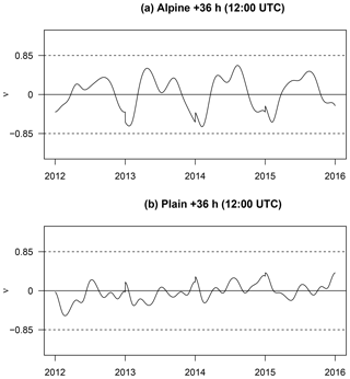
Figure 5 Joint time series of the empirical skewness ν of the forecasted skewed logistic distribution for a lead time of +36 h for the Alpine station (a) and plain site (b) for all four cross-validation blocks. The years on the abscissa correspond to the left-out year of the cross-validation. Symmetric forecasts (no additional skewness required) would show a value of zero. The two dashed lines at $\mathit{\nu }=[-\mathrm{0.85},\mathrm{0.85}]$ are somewhat arbitrary and are shown to facilitate orientation and to match the examples in Fig. 1.

Fig. 5a shows a joint time series of the empirical skewness for the skewed logistic models for all +36 h forecasts (12:00 UTC) over the whole validation period. The estimated seasonal effect for skewness based on the 4-fold cross-validation is plotted against the left-out year, the year which has not been used when estimating the model. Thus, the effects for the four years (2012–2015) look slightly different as they are based on four different models. However, the overall pattern across years is similar, which is an indication that this is a rather persistent characteristic given the data set used in this study. For all years the predictions are positively skewed during the summer season with values of around 0.6. On the contrary, strong negative skewness with values of −0.8 can be seen during the winter season. The consideration of this seasonally dependent skewness yields an overall better performance compared with the Gaussian model.

3.2 Alpine vs. plain site

To see the benefits of a nonsymmetric response distribution in a different environment, the same study is shown for a selected plain site (large square Fig. 2; right column Fig. 3).

Similar to the Alpine site, a pronounced diurnal cycle is visible for all models in terms of LS and CRPS (Fig. 3) with better scores for nighttime. In contrast to the Alpine site, a clear decrease in the forecast performance with increasing lead time can be seen; however, the two heavy-tailed models (logistic and skewed logistic) are still able to improve sharpness (80 % PIW) and calibration (RI) for particular lead times. The estimated skewness is also smaller than for the Alpine site, as shown in Fig. 5. Additionally, the change in sign of the skewness between summer and winter is almost absent. Skewness is still present, but the amplitude is strongly decreased compared with the results for the Alpine site with values of close to zero (symmetric). Even if the improvements over the symmetric logistic models are only minor, the additional skewness still yields slightly better results, especially for short lead times.

In comparison with the Alpine site, the plain site shows an overall better forecast performance for all measures except for RI where both stations show similar scores indicating that both stations are, on average, well calibrated. Moreover, almost all scores (LS, CRPS, and PIW) are smaller than for the Alpine site even for the longest lead time. This is mainly due to the overall better performance of the NWP for regions with no or few topographical features. In such situations the overall performance of the NWP is already adequate and the EPS provides covariates containing more information. Thus, the benefit of the statistical post-processing is much smaller compared with sites in complex terrain. In this example the Gaussian assumption seems to be an appropriate choice, and the improvements of the logistic or skewed logistic distribution are only minor.

3.3 Comparison for all sites

Figure 6 shows averaged scores for LS, CRPS, the mean 80 % PIW, and RI for the three different groups of stations including all 27 sites used in this study (cf. Fig. 2). Each box and whiskers contains the mean score for the individual stations and all 15 lead times. This yields 12×15 values for group “Alpine”, 6×15 for group “foreland”, and 9×15 for group “plain”. In addition, the numeric values of all medians are provided in Table 2 along with median values for two alternative PIWs (50 % and 95 %) and the prediction interval coverage (PIC) for the same three intervals. The validation shows increasing forecast performance with decreasing topographical complexity (top down) independent of the statistical model.

Figure 6 Performance measures in terms of LS, CRPS, 80 % PIW, and RI (left to right), clustered for Alpine, foreland, and plain sites (top to bottom). The box and whiskers are based on average scores for each station and lead time, with the boxes illustrating the interquartile range (0.25–0.75), the whiskers denoting ±1.5 times interquartile range, and the solid circles representing outliers.

Figure 7 As in Fig. 6, but showing the improvement against the classical Gaussian model. Note that improvements are reported by positive values. Differences are shown for LS, whereas skill scores (in %) are shown for CRPS, the 80 % PIW, and the RI.

Table 2 Median of (left to right) the logarithmic score (LS), the continuous ranked probability score (CRPS), the reliability index (RI), and three prediction intervals (PIs) reporting the prediction interval width (PIW) and the prediction interval coverage (PIC) for Alpine, foreland, and plain sites (top to bottom), evaluated for each model type (Gaussian, logistic, and skewed logistic).

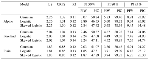
Figure 7 shows the improvements using non-Gaussian distributions, compared with the Gaussian reference model: positive values indicate that the alternative model show an improvement over the Gaussian model. The model results using the symmetric/skewed logistic distribution show minor improvements in terms of LS but can clearly reduce the 80 % PIW without a loss in RI, except at Alpine sites where the logistic model shows a loss in RI (not as well calibrated). CRPS reports barely any difference between the different response distributions for all three groups. Large parts of the improvements can be attributed to the increased sharpness (PIW), which also yields a smaller LS overall without decreasing calibration in terms of RI.

3.4 Comparison to sliding training window

In the following, the long-term training approach presented using 3 years of training data (2012, 2013, and 2014) is compared to the widely used sliding window approach utilizing only the previous 30 or 60 d for training. The validation period chosen is 2015 in order to have at least 1 year of out-of-sample data. Skewed logistic models are not estimated for sliding windows. Due to the parametrization of the skewed logistic distribution and the relatively short training periods, reliable parameter estimates can no longer be ensured; therefore, only results for the Gaussian and logistic models are shown. The estimation of all sliding window models is based on the R package “crch” (Messner et al., 2016) using either minimum CRPS or maximum likelihood optimization (cf., Gebetsberger et al., 2018).

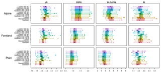
Figure 8 Performance measures in terms of LS, CRPS, 80 % PIW, and RI (left to right), clustered for Alpine, foreland, and plain sites (top to bottom), and were only evaluated on 2015 for out-of-sample comparison. The box and whiskers are based on average scores for each station and lead time, with boxes illustrating the interquartile range (0.25–0.75), whiskers displaying the ±1.5 times interquartile range, and solid circles representing outliers. Sliding training window models are labeled as S60 and S30 denoting a 60 or 30 d training period, respectively. Additionally, the optimization score used is labeled as CRPS or ML (continuous ranked probability score or maximum likelihood), respectively.

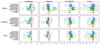
Figure 9 As in Fig. 8, but showing the improvements against the skewed logistic model. Note that improvements are reported by positive values. Differences are shown for LS, whereas skill scores (in %) are shown for CRPS, the 80 % PIW, and the RI.

Figures 8 and 9 show overall scores and skill scores as in the previous subsection. The long-term approach using 3 years of training data shows the smallest LS and CRPS values for the entire validation period. Sharpness in terms of 80 % PIW is lowest for sliding window models. In particular, the sharpness is clearly lower than for long-term training models at Alpine sites. Moreover, the PIW is lower for short (30 d) than for longer (60 d) windows, especially for the 30 d sliding window models at the expense of calibration (RI). RI values report similar behavior, with 60 d sliding windows reporting smaller RI values than 30 d windows. As this verification is solely based on 1 year, there is large variation in the RI values, which is based on PIT histograms.

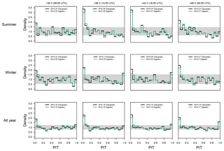
Figure 10 PIT histograms at the Alpine site for the Gaussian (black/dark line) and logistic (green/bright line) sliding 60 d models using CRPS optimization for the 2 d ahead forecasts (left to right: 06:00, 12:00, 18:00, and 00:00 UTC) corresponding to forecasts +30, +36, +42, and +48 h ahead. From the top down, the PIT histograms are shown for summer only (June/July/August), winter only (December/January/February), and for the whole year. The gray horizontal bar shows the point-wise 95 % confidence interval around 1 which indicates perfect calibration.

Therefore, Fig. 10 illustrates a representative PIT for the Alpine site, evaluated for the 60 d sliding window model using CRPS optimization, over the entire data period from March 2012 to the year 2015 (4 years minus 60 d). A distinct U-shape can be identified in the all year verification with peaks in the lowest and highest PIT bins. In particular, the sliding window approach shows a large peak in the lowest bin during summer, which also indicates residual skewness. Similar behavior is visible for winter periods, although it is less pronounced. The 60 d sliding window models using the maximum likelihood estimation decreases these peaks and yields more well-calibrated PITs (not shown) as they are less prone to being overconfident (Gebetsberger et al., 2018).

4 Summary and conclusion

Nonhomogeneous regression is a widely used statistical method for post-processing numerical ensemble forecasts. It was originally developed to improve probabilistic air temperature forecasts and assumes a Gaussian response distribution.

However, several studies have shown that marginal temperature distributions can be skewed or nonsymmetric, respectively (Warwick and Curran, 1993; Harmel et al., 2002). This marginal skewness can result from topographically induced effects such as cold pools during winter or a strong valley bottom heating within narrow valleys on hot summer days. Thus, skewness is much stronger for locations surrounded by complex terrain than for sites in plain regions.

Moreover, skewness is supposed to decrease if additional covariates (e.g., individual ensemble members, seasonal effect, and different ensemble forecast quantities) are included in the Gaussian model (see, e.g., Messner et al., 2017). However, the calibration of the results presented in this article indicate that residual skewness remains, even when including more variables than just the ensemble temperature covariate. Thus, the skewness might need to be included using an appropriate response distribution without increasing the model complexity with additional covariates. Such covariates would also require variable selection techniques to avoid overfitting.

In this study, the skewed logistic distribution was used and compared to the (symmetric) logistic and Gaussian distributions for probabilistic post-processing of the 2 m air temperature at 27 sites in central Europe for stations in three different environments: Alpine, foreland close to the Alps, and sites located in plain regions. The skewed logistic distribution allows one to directly handle possible skewness in the data, if needed.

The two logistic distributions perform better for 1 d up to 4 d ahead forecasts for the majority of the stations and lead times – in particular regarding sharpness and logarithmic score (LS) – without decreasing calibration, which is analyzed by the reliability index (RI) and probability integral transform (PIT) histograms. The amount of improvement decreases with the decreasing complexity of the topography.

When PIT histograms are used to check for calibration, they have to be checked for different seasons, lead times, and hours of day. Averaging over the whole year or multiple times of the day may mask shortcomings especially in complex terrain, and the distinct patterns as shown in the results might easily be overlooked.

A comparison to sliding window models, where a fixed number of previous days is used for training, highlights that the sliding window approach obtains sharp forecasts, but results in uncalibrated forecasts regarding PIT histograms. A longer sliding window of 60 d compared with 30 d decreases the sharpness of the probabilistic forecasts; however, it is still not calibrated and indicates that skewness occurs in the residuals. Consequently, longer training windows would have even larger issues with residual skewness. To overcome this, the current study uses a long-term training approach of 3 years and accounts for seasonality. This additional seasonality reduces most parts of the skewness, but still improves the sharpness without decreasing calibration.

The sliding training approach has the advantage of being able to react to and account for changes in the ensemble model quickly if two statistically different time periods exist. The long-term approach would need a refitting of the regressions coefficients for the new period after a change occurred, or the change would have to be treated in the statistical models if two periods are mixed during training.

In conclusion, the Gaussian assumption for probabilistic temperature post-processing may be appropriate for regions where the ensemble provides sufficient information regarding the marginal distribution of the response. However, if the covariates used in the regression model miss some features, residual skewness becomes challenging. An alternative response distribution, such as the proposed skewed logistic distribution, allows one to directly address unresolved skewness and increases the predictive performance of the probabilistic forecasts.

Appendix A: Skewness of the skewed logistic distribution

The third moment (skewness, ν) is a function of the shape parameter ζ:

$$\begin{array}{}\text{(A1)}& \mathit{\nu }\left(\mathit{\zeta }\right)={\displaystyle \frac{{\mathrm{\Psi }}^{\prime \prime }\left(\mathit{\zeta }\right)-{\mathrm{\Psi }}^{\prime \prime }\left(\mathrm{1}\right)}{\left({\mathrm{\Psi }}^{\prime }\right(\mathit{\zeta })+{\mathrm{\Psi }}^{\prime }(\mathrm{1}){)}^{\frac{\mathrm{3}}{\mathrm{2}}}}},\end{array}$$

where Ψ^′ and Ψ^′′ denote the first and second derivative of the polygamma function Ψ(x) (Abramowitz and Stegun, 1965, Sect. 6.4.1, p. 260) defined as

$$\begin{array}{}\text{(A2)}& \mathrm{\Psi }\left(x\right)={\displaystyle \frac{{\mathrm{\Gamma }}^{\prime }\left(x\right)}{\mathrm{\Gamma }\left(x\right)}}.\end{array}$$

Here, Γ(x) denotes the Gamma function (Abramowitz and Stegun, 1965, Sect. 6.1.1, p. 255) and Γ^′(x) is its first derivative. The Gamma function is defined as

$$\begin{array}{}\text{(A3)}& {\displaystyle }\mathrm{\Gamma }\left(x\right)=\underset{\mathrm{0}}{\overset{\mathrm{\infty }}{\int }}{t}^{x-\mathrm{1}}\exp (-t)\mathrm{d}t.\end{array}$$