the Creative Commons Attribution 4.0 License.
the Creative Commons Attribution 4.0 License.
 | 06 Oct 2020
The effect of geographic sampling on evaluation of extreme precipitation in high-resolution climate models
Michael F. Wehner
Traditional approaches for comparing global climate models and observational data products typically fail to account for the geographic location of the underlying weather station data. For modern global high-resolution models with a horizontal resolution of tens of kilometers, this is an oversight since there are likely grid cells where the physical output of a climate model is compared with a statistically interpolated quantity instead of actual measurements of the climate system. In this paper, we quantify the impact of geographic sampling on the relative performance of high-resolution climate model representations of precipitation extremes in boreal winter (December–January–February) over the contiguous United States (CONUS), comparing model output from five early submissions to the HighResMIP subproject of the CMIP6 experiment. We find that properly accounting for the geographic sampling of weather stations can significantly change the assessment of model performance. Across the models considered, failing to account for sampling impacts the different metrics (extreme bias, spatial pattern correlation, and spatial variability) in different ways (both increasing and decreasing). We argue that the geographic sampling of weather stations should be accounted for in order to yield a more straightforward and appropriate comparison between models and observational data sets, particularly for high-resolution models with a horizontal resolution of tens of kilometers. While we focus on the CONUS in this paper, our results have important implications for other global land regions where the sampling problem is more severe.
- Article
(13513 KB) - Full-text XML
- BibTeX
- EndNote


This manuscript has been authored by an author at Lawrence Berkeley National Laboratory under Contract No. DE-AC02-05CH11231 with the U.S. Department of Energy. The U.S. Government retains, and the publisher, by accepting the article for publication, acknowledges, that the U.S. Government retains a non-exclusive, paid-up, irrevocable, world-wide license to publish or reproduce the published form of this manuscript, or allow others to do so, for U.S. Government purposes.
Global climate models can contain significant uncertainties, particularly in their characterization of precipitation extremes. As a result, it is critical to use observation-based data sets to evaluate a particular climate model to assess if the model is fit for purpose in exploring extremes and, if so, where and when the model is either acceptable or unacceptable for characterizing extreme precipitation. Traditionally, gridded daily products are used as a “ground truth” data set for evaluating a climate model because (1) these data products are based on measurements of the real world (e.g., in situ measurements or satellite observations) and (2) they enable a like-for-like comparison between climate models and observations. However, in geographic regions with sparse sampling by weather stations, gridded products do not represent actual measurements of daily precipitation; instead, they represent a statistical interpolation of the sparse measurements. The underlying physics of a climate model, on the other hand, yield a process-based characterization of, for example, extreme precipitation for every grid cell. Consequently, a comparison of the climate model output versus a gridded product over an area with poor observational sampling (e.g., regions with large orographic variability) could be misleading. This issue has already been examined in constructions of global mean temperature trends from station data (Madden and Meehl, 1993; Vose et al., 2005), although the effects of geographic sampling were minor partly because of the great care taken in the construction of trends (Jones et al., 2001).
One way to ensure that a comparison of climate model output is conducted against real measurements of the Earth system is to consider only model grid cells with at least one representative high-quality station (the standard of comparison we use in this paper; see Sect. 3.2). For modern global climate models such as CESM2 (Bacmeister et al., 2020) and CanESM5 (Swart et al., 2019), the horizontal resolution is coarse enough that a large majority of grid cells over the contiguous United States (CONUS) meet this criterion (in fact, all grid cells contain at least one representative station for CanESM5). However, the story is much different for high-resolution global climate models with a horizontal resolution of tens of kilometers – the evaluation of which is the primary motivation for this paper. For example, when considering model output from five early submissions to the HighResMIP subproject of the CMIP6 experiment (Haarsma et al., 2016), the finer horizontal resolution means that at most 60 % of the grid cells over CONUS contain a representative station (see Table A1). An extreme example is the HadGEM3-GC3.1-HM model (Roberts et al., 2019, which has a ∼20 km horizontal resolution), for which only 22 % of the model grid cells contain a representative station. In other words, for this particular selection criterion, accounting for geographic sampling with CanESM5 would have no impact on the assessment of model performance, because all grid cells (each about ∼300 km across) have at least one high-quality station over the CONUS region. On the other hand, one might expect that the model performance could change drastically for the HadGEM3-GC3.1-HM model.
In this paper, we make the case that geographic sampling of observational data should be taken into consideration when comparing climate model representations of extremes to observations, particularly for high-resolution models with a horizontal resolution of tens of kilometers. To this end, we develop a framework for systematically quantifying the effect of geographic sampling via a “true” standard of comparison based only on the model grid cells with a corresponding high-quality weather station. Our metrics for making this comparison are a measure of extreme bias and Taylor diagrams (Taylor, 2001), which summarize the spatial pattern correlation and variability after removing any biases. For extreme precipitation in boreal winter (DJF) over the contiguous United States (CONUS), we find that properly accounting for the geographic sampling of weather stations can significantly change the assessment of model performance. While we explore the CONUS in this paper, the geographic sampling issue is particularly important when considering global regions with very limited sampling (e.g., Central Asia, South America, or Africa).
Before proceeding with our analysis, it is important to highlight several key points with respect to observational data products and the proper methodology for conducting model comparison for precipitation extremes. On the one hand, in addition to the fact that daily gridded products are convenient for model comparison, it has been clearly documented that they are the best observational data source to use for yielding a like-for-like comparison with climate models for precipitation extremes (e.g., Chen and Knutson, 2008; Gervais et al., 2014). This is based on the fact that the correct interpretation for model grid cell precipitation is an areal average and not a point measurement (see, e.g., Chen and Knutson, 2008). Of course, weather stations yield point measurements, and daily gridded products that are based on an interpolation scheme or “objective analysis” should be interpreted as a point measurement (e.g., Livneh et al., 2015b). However, when the native resolution of a gridded product is sufficiently finer than that of the climate model of interest, gridded point measurements can still be used for model evaluation of precipitation extremes so long as a specific workflow is followed; see Gervais et al. (2014).
On the other hand, as a purely observational product, a recent thread of research argues that gridded daily products are an inappropriate data source for characterizing pointwise measurements of extreme precipitation. The reasoning here is that daily precipitation is known to exhibit fractal scaling (see, e.g., Lovejoy et al., 2008; Maskey et al., 2016, and numerous references therein), and therefore any spatial averaging during the gridding process will diminish variability and extreme values. A number of analyses specifically document this phenomena (King et al., 2013; Gervais et al., 2014; Timmermans et al., 2019); for example, Risser et al. (2019b) show that daily gridded products underestimate long-period return values by 30 % or more relative to in situ measurements. Gridded point-based extreme-precipitation data products like Donat et al. (2013) or Risser et al. (2019b) preserve the extreme statistics of weather station measurements, but since they are not flux conserving and furthermore do not account for the temporal occurrence of extreme events over space, they can only provide local information about the climatology of precipitation extremes. Such products are very useful for characterizing the frequency of extreme precipitation for local impact analyses, but they are by construction an unsuitable data source for conducting model evaluation or comparison.
As a final note, we emphasize that in this paper we limit any comparisons to each individual model, focusing on the geographic sampling question, and specifically do not conduct intercomparisons with respect to ranking the models or providing general conclusions about their relative performance. Since high-resolution global climate models are the focus of this work, as previously mentioned, we utilize output from several HighResMIP models with horizontal resolutions of ∼25 to ∼50 km. However, the HighResMIP protocol (outlined in Haarsma et al., 2016) is unique, because it has been designed to systematically investigate the impact of increasing horizontal resolution in global climate models. To that end, the various modeling centers performed two simulations at two spatial resolutions for each model. The HighResMIP protocol recommends that only the lower-resolution version of the model should be tuned and that the same set of parameters should be used, as far as possible, in the simulation at high spatial resolution. Therefore, the high-resolution simulations (which are the simulations used in this study) have not been designed to be the best possible simulations of each individual model, even if they have generally been performed using the latest version of each model. This is particularly important for precipitation extremes that are strongly influenced by moist physics parameterizations.
The paper proceeds as follows: in Sect. 2 we describe the various data sources used (gridded daily products and climate model output) in our analysis, and in Sect. 3 we describe the statistical methods and framework for accounting for geographic sampling. In Sect. 4, we illustrate our methodology using a case study comparing a well-sampled (spatially) region versus a poorly sampled region before presenting the results of our analysis for all of CONUS, maintaining a focus on boreal winter (DJF) precipitation. Section 5 concludes the paper.
2.1 Observational reference data
As described in Sect. 1, model-simulated precipitation is best interpreted as an areal average over the model grid cell (Chen and Knutson, 2008; Gervais et al., 2014) as opposed to the point-measurement interpretation appropriate to in situ weather station measurements. Following Gervais et al. (2014), the correct way to compare model data with station data for precipitation extremes is as follows: (1) use an objective analysis to translate daily station measurements to a grid with a much higher resolution than the model resolution, (2) use a conservative remapping procedure (e.g., Jones, 1999) to translate the daily high-resolution grid values to the climate model grid, and (3) calculate the extreme statistics of interest.
One pre-existing gridded product that meets the criteria of step 1 above is the Livneh et al. (2015a, b) daily gridded product (henceforth L15), which has been gridded to a 1∕16∘ or ∼6 km horizontal resolution and spans the period 1950–2013. While the data product covers North America (south of 53∘ N), we limit our consideration to those grid cells within the boundaries of the contiguous United States (CONUS). The L15 data product takes in situ measurements of daily total precipitation (over CONUS, the input data are from the Global Historical Climatology Network; Menne et al., 2012) and creates a daily gridded product by first interpolating daily station measurements to a high-resolution grid and then applying a monthly scaling factor calculated from the topographically aware PRISM data product (Daly et al., 1994, 2008). While the combination of interpolating point measurements and applying a monthly rescaling likely has an impact on observed extreme events, such considerations are beyond the scope of this paper.
For each of the climate model grids considered (see Table 1), we first regrid the daily L15 data to the model grid using a conservative remapping procedure (we utilize functionality from the rainfarmr package for R; von Hardenberg, 2019) and then extract the largest running 5 d precipitation total (denoted Rx5Day) in each DJF season at each grid cell, which is denoted as
where Y represents the Rx5Day value, the superscript “obs” indicates observations, t is the year, g is the grid cell, and 𝒢m is the model grid for model .
The L15 data product is, of course, only one of a very large number of gridded daily precipitation products that could be considered in this study. However, we choose to use L15 for several reasons: first, it is one of the more widely used gridded daily products; second, it covers a relatively long time record (64 years); and finally, its native resolution is sufficiently higher than the climate models considered in this paper such that it can be conservatively remapped to the model grids following the procedure outlined in Gervais et al. (2014). The Climate Prediction Center (CPC) 0.25∘ × 0.25∘ daily US unified gauge-based analysis of precipitation is another commonly used data product with similar time coverage; however, its 0.25∘ resolution is approximately the same as the models considered in this study. Since the CPC product represents a point measurement, its resolution is too coarse to be appropriately translated to an areal average for use in HighResMIP model evaluation according to the Gervais et al. (2014) methodology.
Table 1HighResMIP climate model output used in the analyses for this paper.
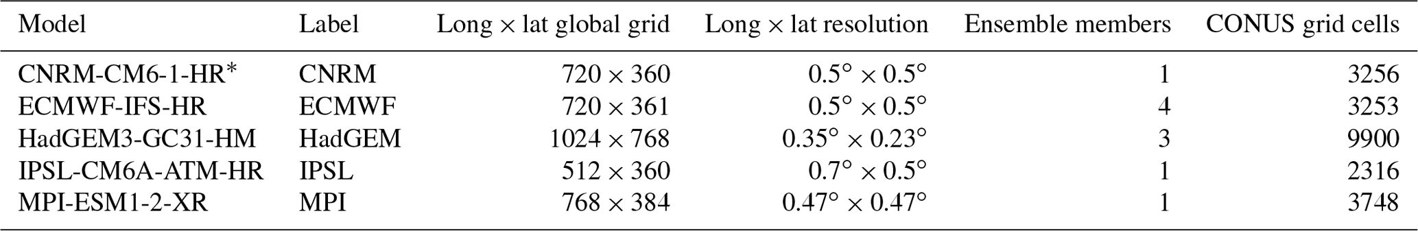
∗ Note that the CNRM runs are only from 1981 to 2014.
2.2 Climate models
Given that this study is motivated by the evaluation of high-resolution climate models with horizontal resolutions of tens of kilometers, we utilize early submissions to the high-resolution simulation with fixed sea surface temperatures covering 1950–present (highresSST–present) experiment of the HighResMIP subproject of the CMIP6 experiment (Haarsma et al., 2016), all of which are atmospheric model intercomparison project (AMIP)-style runs with fixed sea surface temperatures from 1950 to 2014. As mentioned in Sect. 1, the HighResMIP protocol was designed to systematically explore the impact of increasing horizontal resolution in global climate models. Each of the models used here was run at two spatial resolutions, including a high spatial resolution. However, the protocol specifies that only the low-resolution version of the model is tuned and that the same set of parameters is used for the high-resolution simulations. We utilize only the high-resolution simulations, even though several of the models have scale-aware parameterizations (i.e., they have to be modified with increasing resolution); therefore, there might be large differences between the models in terms of the tuning used in the simulations evaluated here. For this reason, we reiterate that in this paper we maintain comparisons to within-model statements and do not attempt to conduct intercomparison.
The following models are used for our analysis.
-
CNRM-CM6-1-HR is developed jointly by CNRM-GAME (Centre National de Recherches Météorologiques – Groupe d'études de l'Atmosphère Météorologique) in Toulouse, France, and CERFACS (Centre Européen de Recherche et de Formation Avancée); see Voldoire et al. (2013). Data are interpolated to a regular 720×360 (0.5∘ × 0.5∘) longitude–latitude grid from the native T359l reduced Gaussian grid. The model has 91 vertical levels with the top level at 78.4 km.
-
ECMWF-IFS-HR is the Integrated Forecasting System (IFS) model of the European Centre for Medium-Range Weather Forecasts as configured for multidecadal ensemble climate change experiments (Roberts et al., 2018). Data are interpolated to a regular 720×361 (0.5∘ × 0.5∘) longitude–latitude grid from the native Tco399 cubic octahedral reduced Gaussian grid (nominally ∼25 km). The model has 91 vertical levels with the top model level at 1 hPa.
-
HadGEM3-GC31-HM is the UK Met Office Hadley Centre (Exeter, United Kingdom) unified climate model, HadGEM3-GC3.1-HM on a regular 1024×768 (0.35∘ × 0.23∘) longitude–latitude grid (nominally 25 km; Roberts et al., 2019). The model has 85 vertical levels with the top model level at 85 km.
-
IPSL-CM6A-ATM-HR is developed by the Institut Pierre Simon Laplace in Paris, France (Boucher et al., 2019). Data are interpolated from the native N256 geodesic grid to a 512×360 (0.7∘ × 0.5∘) longitude–latitude grid (nominally ∼50 km). The model has 79 vertical levels with the top model level at 40 000 m.
-
MPI-ESM1-2-XR is the Max Planck Institute for Meteorology in Hamburg, Germany (Gutjahr et al., 2019). Data are interpolated to a regular 768×384 (0.47∘ × 0.47∘) longitude–latitude grid (nominally ∼50 km) from the native T255 spectral grid. The model has 95 vertical levels with the top model level at 0.1 hPa.
For each of these models (additional details are provided in Table 1) and each ensemble member, we calculate the corresponding DJF Rx5Day values for each ensemble member in each grid box over CONUS. Furthermore, note that we mask out grid cells that are not fully over land. These values are denoted
for model , where 𝒢m is the model grid for model m, and Nens,m is the number of ensemble members for model m (see Table 1); however, note that the CNRM runs only cover 1981–2014.
3.1 Extreme value analysis
The core element of our statistical analysis is to estimate the climatological features of extreme precipitation for the regridded L15 and each climate model using the generalized extreme value (GEV) family of distributions, which is a statistical modeling framework for the maxima of a process over a prespecified time interval or “block”, e.g., the 3-month DJF season used here. Coles et al. (2001) (Theorem 3.1.1, p. 48) shows that when the number of measurements per block is large, the cumulative distribution function (CDF) of the seasonal Rx5Day Yt(g) can be approximated by a member of the GEV family:
which is defined for . The GEV family of distributions (Eq. 1) is characterized by three space-time parameters: the location parameter μt(g)∈ℛ, which describes the center of the distribution; the scale parameter σt(g)>0, which describes the spread of the distribution; and the shape parameter ξt(g)∈ℛ. The shape parameter, ξt(g), is the most important for determining the qualitative behavior of the distribution of daily rainfall at a given location. If ξt(g)<0, the distribution has a finite upper bound; if ξt(g)>0, the distribution has no upper limit; and if ξt(g)=0, the distribution is again unbounded and the CDF (Eq. 1) is interpreted as the limit ξt(g)→0 (Coles et al., 2001). While the GEV distribution is only technically appropriate for seasonal maxima as the block size approaches infinity, Risser et al. (2019a) verify that the GEV approximation is appropriate here even though the number of “independent” measurements of Rx5Day in a season is relatively small, particularly when limiting oneself to return periods within the range of the data (as we consider here, with the 20-year return values).
While our goal is to simply estimate the climatology of extreme precipitation (and specifically not to estimate or detect trends), the nonstationarity of extreme precipitation over the last 50 to 100 years (see, e.g., Kunkel, 2003; Min et al., 2011; Zhang et al., 2013; Fischer and Knutti, 2015; Easterling et al., 2017; Risser et al., 2019a) requires that we characterize a time-varying extreme value distribution. Here, we use the simple trend model:
where Xt=[GMT]t is the smoothed (5-year running average) annual global mean temperature anomaly in year t, obtained from GISTEMPv4 (Lenssen et al., 2019; GISTEMP Team, 2020). The global mean temperature is a useful covariate for describing changes in the distribution of extreme precipitation, although other process-based covariates could work equally well or better (Risser and Wehner, 2017). While this is an admittedly simple temporal model, we argue that it is sufficient for characterizing the climatology of seasonal Rx5Day. Furthermore, Risser et al. (2019a) use a similar trend model as Eq. (2), which they show to be as good (in a statistical sense) as more sophisticated trend models (where, for example, the scale and/or shape vary over time). While it has been argued that much more data are required to fit nonstationary models like Eq. (2) reliably (Li et al., 2019), the inclusion of a single additional statistical parameter is used to address the fact that seasonal Rx5Day over CONUS is not identically distributed over 1950–2013. Furthermore, all comparisons in this paper are based on a time-averaged return value, and we do not attempt to directly interpret any temporal changes in the distribution of Rx5Day. We henceforth refer to μ0(g), μ1(g), σ(g), and ξ(g) as the climatological coefficients for grid cell g, as these values describe the climatological distribution of extreme precipitation in each year.
For each model grid and data type (climate model output or regridded L15), we utilize the climextRemes package for R (Paciorek, 2016) to obtain maximum likelihood estimates (MLEs) of the climatological coefficients, which are denoted as
independently for each grid cell. Within climextRemes, we also utilize the block bootstrap (see, e.g., Risser et al., 2019b) to quantify uncertainty in the climatological coefficients in all data sets considered. For those models with more than one ensemble member (see Table 1), we treat the ensemble members as replicates and obtain a single MLE of the climatological coefficients. The MLEs from Eq. (3) and the bootstrap estimates can be used to calculate corresponding estimates of the DJF climatological 20-year return value, denoted , which is defined as the DJF maximum five-daily precipitation total that is expected to be exceeded on average once every 20 years in grid cell g under a fixed GMT anomaly. In other words, is an estimate of the quantile of the distribution of DJF maximum five-daily precipitation at grid cell g, i.e., , which can be written in closed form in terms of the climatological coefficients:
(Coles et al., 2001); here is the average GMT anomaly over 1950 to 2013. Averaging over the GMT values yields a time-averaged or climatological estimate of the return values.
At the end of this procedure, we have MLEs of the climatological 20-year return value for each of the five climate models and each of the five regridded L15 data sets, as well as bootstrap estimates of these return values, , for each model grid and data type.
3.2 Comparing the climatology of extreme precipitation
We illustrate the effect of geographic sampling on the evaluation of simulated 20-year return values of winter (DJF) maximum 5 d precipitation from selected high-resolution climate models with Taylor diagrams (Taylor, 2001) to illustrate pattern errors and return value bias to quantify magnitude errors. Taylor diagrams (Taylor, 2001) plot the centered pattern correlation between observations and simulations as the angular dimension and the ratio of the observed to simulated spatial standard deviation as the radial dimension. These diagrams provide information about the spatial pattern of model errors with the biases removed. The bias in 20-year return values (hereafter referred to as “extreme bias”), defined as the absolute difference between the return values from model and observations, provides a simple measure of whether the models are too dry or too wet, while the Taylor diagram provides three useful metrics displayed in a single plot: (1) the spatial pattern correlation between the model and observations, (2) a comparison of the spatial standard deviation over the region, and (3) a skill score to assess a level of agreement between the two spatial fields. Taylor's modified skill score 𝒮, comparing two spatial fields (e.g., model versus observations), is defined as
where sj is the standard deviation of spatial field , and r is the spatial pattern correlation between the two fields (also used in Wehner, 2013). The skill score essentially involves the ratio of the mean squared error between the two fields (after removing the average from each field) and the standard deviations of each field; the score 𝒮 ranges between 0 (indicating low skill) and 1 (indicating perfect skill). Further details on the Taylor diagrams are provided in Sect. 4; however, an important detail is that to calculate a Taylor diagram we must have “paired” observations and model data; i.e., both data sources must be defined on the same spatial support or grid, which fits nicely into the framework considered in this paper.
In order to illustrate the effect of geographic sampling, we can compare the extreme bias and Taylor diagram results for two approaches.
- A1
True model performance. First, in what we regard as the true performance for each model, we calculate the extreme bias and Taylor diagram metrics using the subset of model grid cells (for the model and regridded L15) that have corresponding weather station measurements. L15 is based on measurements from the GHCN-D (Menne et al., 2012) records, but its stability constraint (selecting stations with a minimum of 20 years of data over CONUS; Livneh et al., 2015b) means that the specific station measurements that go into the daily gridded product change over time. To navigate this complication, we define a set of “high-quality” stations from the GHCN to be those stations that have at least 90 % non-missing daily measurements over 1950–2013. This results in n=2474 stations with a relatively good spatial coverage of CONUS (see Fig. A1), although the coverage is much better in the eastern United States relative to, for example, the Mountain West (see Fig. A9). The 90 % threshold is somewhat arbitrary, but this cutoff ensures that these stations enter into the L15 gridding procedure for a large majority of days over 1950–2013. Next, for each model grid, we identify the grid cells that have at least one high-quality GHCN station (see Fig. A2 in the appendix). The extreme bias and Taylor diagram are then calculated for only those grid cells with at least one high-quality station. Since this comparison isolates the regridded L15 cells that actually involve a real weather station measurement, we regard this as the true extreme bias and Taylor diagram metrics for each model.
- A2
Ignore geographic sampling. To assess how the performance of each model changes when the geographic sampling of weather stations is not accounted for, we calculate the extreme bias and Taylor diagram metrics using all grid cells.
Approach A1 provides us with a standard of comparison, since it properly accounts for the geographic sampling of the underlying weather stations, and we argue that this is the most appropriate way to conduct model comparison. Approach A2, on the other hand, is what would be done without consideration for the geographic sampling issue. Comparing the extreme bias and Taylor diagrams for A1 versus A2 allows us to explicitly quantify the effect of geographic sampling on assessed model performance.
For reference, we have provided a supplemental figure for each model that shows the estimated 20-year return values for the climate model output and regridded L15, the corresponding bootstrap standard errors, the absolute difference in return values, and the ratio of standard errors for the climate model vs. regridded L15; see Figs. A3, A4, A5, A6, and A7.
4.1 Case study: Kansas versus Utah
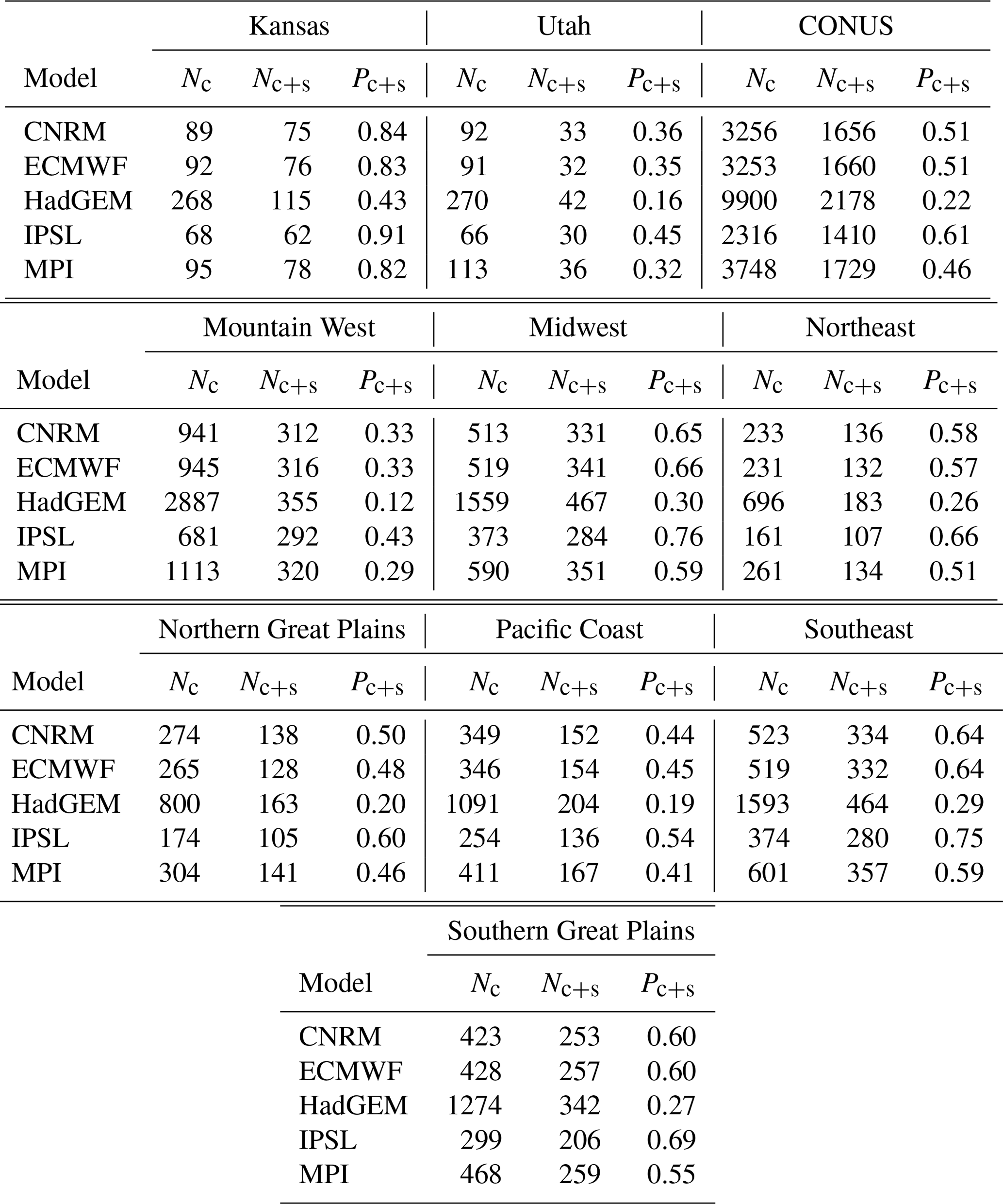
To illustrate our methodology, we first explore return value estimates for two small spatial subregions that exhibit very different sampling by the GHCN network, namely, Kansas and Utah. These two states present an illustrative case study for our method because Utah is poorly sampled (52 stations over 219 890 km2), while Kansas is well sampled (140 stations over 213 100 km2). Figure 1 shows the model grid cells with and without at least one high-quality station. In Kansas, there are anywhere from 40 % (HadGEM) to 90 % (IPSL) of the model grid cells with a high-quality station; in Utah, between 16 % (HadGEM) and 45 % (IPSL) of the model grid cells have a high-quality station (see Table A1 in the appendix). The L15 climatology of 20-year return values is quite similar in these two states: the median return value (interquartile range) in Kansas is 53.8 mm ([39.4,61.0]), while in Utah the median is 49.6 mm ([34.3,71.1]).
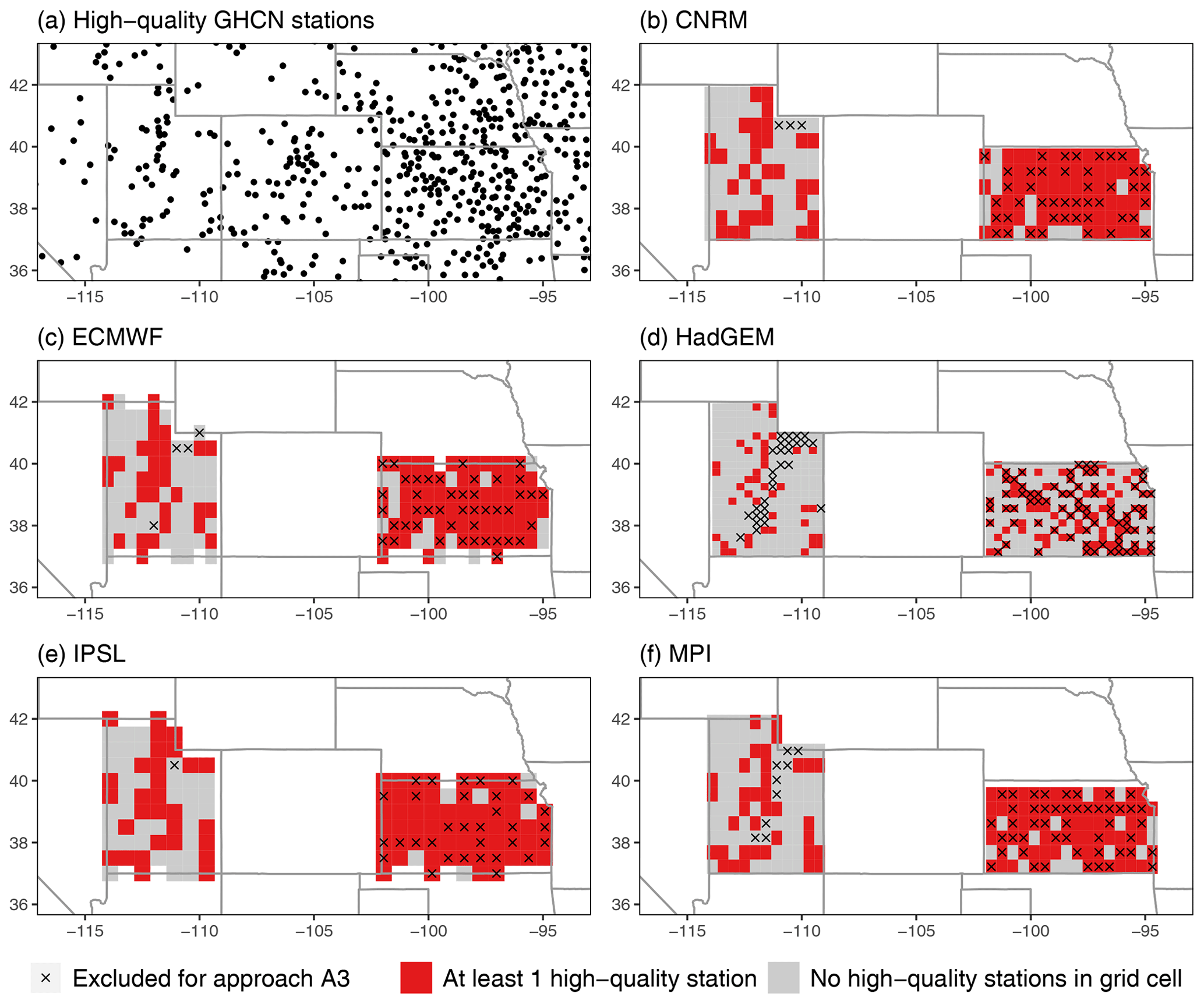
Figure 1Model grid cells with at least one high-quality GHCN station for Kansas and Utah, with an × denoting model grid cells that are excluded for A3KS and A3UT.
However, Utah also differs markedly from Kansas with respect to topography: Kansas is relatively flat, while Utah exhibits complex orographic variability. While the geographic sampling of stations is likely decoupled from rainfall behavior in Kansas, in Utah stations are primarily located at lower elevations where extreme orographic precipitation does not occur. Indeed, the median elevation of the high-quality stations in Utah is around 1600 m (the highest station is at 2412 m), while the highest peaks in Utah exceed 4000 m. When considering the model grids, the geographic sampling of the weather stations excludes the highest elevations for all models except IPSL, which has the coarsest resolution of those considered in this paper. For example, looking at the relationship between the average elevation of each grid cell (averaged from the GTOPO30 1 km digital elevation data set) and the 20-year return values for both the model output and L15 (see Fig. A8 in the appendix), it is clear that grid cells with the highest elevations in Utah do not have a corresponding high-quality station. On the other hand, this phenomena is nearly irrelevant for Kansas (as expected), since the unsampled model grid cells mostly fall within the elevation range of the sampled cells.

Figure 2Extreme bias (difference in 20-year return values of Rx5Day) in Kansas and Utah for each model (model minus regridded L15) and approaches A1, A2, and A3 (a), with the difference in extreme bias (in mm) for approach A2 (ignoring geographic sampling) versus A1 and approach A3 (assessing the effect of sampling density for Kansas and orography for Utah) versus A1 (b). All estimates show the 90 % basic bootstrap confidence intervals.
The implication here is that any relative differences between approaches A1 and A2 for Kansas versus Utah could be due to either the different geographic sampling of the two states or orographic considerations (or both). To explicitly separate these two possibilities, we introduce a third approach for the case study (denoted A3). Given the differences in Kansas and Utah (with respect to sampling density and orography), we define this approach differently for each state:
- A3KS
-
Consider a subset of grid cells with a high-quality station. The difference between A1 and A2 in Kansas is going to be minimal for many of the models simply because the state is extremely well sampled (CNRM, ECMWF, IPSL, and MPI all have greater than 80 % of their model grid cells with a representative high-quality station). To assess the influence of the high station density in Kansas, we can alternatively compare the performance of each model when we randomly subsample the model grid cells such that the proportion of cells with a high-quality station matches that of Utah. For example, for CNRM, only of the model grid cells have at least one high-quality station in Utah (see Table A1 in the appendix); we can randomly select 32 of the CNRM grid cells in Kansas that have a high-quality station so that the proportion of Kansas sampled matches that of Utah (). In other words, this approach allows us to answer the following question: what would the effect of geographic sampling be for Kansas if its sampling density matched Utah? The grid cells excluded for A3KS are shown in Fig. 1.
- A3UT
-
Ignore geographic sampling but threshold high elevations. For Utah, this approach ignores geographic sampling (like A2) but only considers those model grid cells whose elevation does not exceed the highest grid cell with a high-quality station. For example, for HadGEM, the A3UT approach excludes any model grid cell with an average elevation that exceeds 2380 m (which is the highest grid cell with a high-quality station for the HadGEM grid; see Fig. A8 in the appendix). In other words, this approach allows us to answer the following question: what would the effect of geographic sampling be for Utah if we remove systematic differences in orography? The grid cells excluded for A3UT are also shown in Fig. 1.
The true extreme bias averaged over each state with a 90 % basic bootstrap confidence interval (CI) is shown in Fig. 2a, along with the extreme bias for A2 and A3. In Kansas, the models are uniformly too wet, with positive biases of approximately 10–25 mm in all models and only the CNRM CI significantly overlapping zero. The uncertainty for CNRM is significantly larger than the other models in Kansas, which may be related to the fact that these runs only cover 1981–2014, while the other models cover 1950–2014. In Utah, the models are generally too wet again, and the biases for IPSL and MPI are particularly large. The ECMWF model's dry bias is a notable exception in Utah. The model biases for Kansas are all within each others uncertainties, while the biases across models do not always overlap in Utah.
Turning to the difference in bias in Fig. 2b, there is a minimal effect of geographic sampling in Kansas: the CIs for the difference in extreme bias for A2 versus A1 include zero for all models. Interestingly, this remains true for approach A3KS, where the CIs for A3KS versus A1 still include zero and completely overlap the CIs for A2 versus A1 (although the uncertainty in the A3KS versus A1 difference is extremely large for CNRM). This is also visible in Fig. 2a, where the confidence intervals for the extreme bias under A2 and A3 are essentially identical to that for A1. The story is much different for Utah: while the CIs for the extreme biases under A2 and A3 overlap the CI for the true extreme bias, there appear to be systematic differences for HadGEM, IPSL, and MPI. When looking at a confidence interval for the difference, the CIs for A2 versus A1 do not include zero for HadGEM, IPSL, or MPI. (The fact that the actual extreme bias CIs overlap but the CI for the difference does not include zero is based on the fact that the difference CI is based on bootstrap estimates from paired bootstrap samples.) The implication is that for these models, failing to account for geographic sampling makes each model appear to be drier than it actually is. For CNRM and ECMWF, on the other hand, the best estimate of the difference between A2 and A1 is positive, meaning that ignoring geographic sampling makes the models appear to be too wet (however, their confidence intervals include zero). Considering the A3UT versus A1 changes in extreme bias, there are interesting differences for all models except CNRM. In ECMWF the extreme bias gets larger, which is unusual (although the A2 vs. A1 and A3UT vs. A1 CIs overlap), while the extreme biases decrease in absolute value for HadGEM, IPSL, and MPI. For IPSL and MPI, these decreases are not meaningful (the CIs nearly coincide with one another), and while the HadGEM CIs also overlap, the changes are larger. This might have something to do with model resolution, since the HadGEM model has the highest resolution of those considered in this study.
These two states provide important insights into the effect of geographic sampling with respect to the extreme bias. In Kansas, the changes in extreme bias are nonsignificant even when we artificially reduce the amount of information from the underlying weather stations. The implication is that for relatively homogeneous domains like Kansas the geographic sampling and its density are less important; in other words, to accurately evaluate models, fewer stations are required in topographically flat regions. In Utah, the geographic sampling is much more important since there are significantly nonzero differences in the extreme bias when it is ignored. Accounting for the influence of orography decreases this effect (i.e., the change in bias is generally less for A3UT relative to A2), but the interesting point is that when sampling matters (i.e., when the A2 vs. A1 confidence interval does not include zero) it still matters regardless of whether accounting for elevation or not. A possible exception is ECMWF, for which the A2 vs. A1 CI includes zero, while the A3UT vs. A1 CI does not.
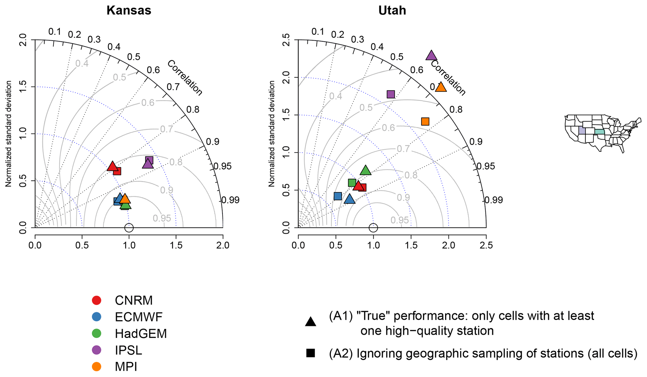
Figure 3Taylor diagrams comparing 20-year return values for Kansas and Utah for the climate models versus regridded L15. The gray curvilinear lines represent the skill score for each model relative to the regridded L15.
The Taylor diagrams comparing 20-year return values for Kansas and Utah are shown in Fig. 3. In light of the results for the extreme bias and in order to not complicate the plot, we have chosen to leave the A3 comparison off of the Taylor diagrams (furthermore, we do not show the uncertainty in the Taylor diagrams, which is again for simplicity). Clearly, as with the extreme bias, the performance of the various climate models in replicating the spatial pattern and variability of extreme precipitation is very different for these two states. In Kansas, all models except IPSL almost perfectly reproduce the spatial variability of the return values, with or without accounting for geographic sampling. ECMWF, HadGEM, and MPI furthermore nearly reproduce the spatial patterns of extreme precipitation (again with or without accounting for geographic sampling), with spatial pattern correlations in excess of 0.95. Across all models the performance is nearly identical regardless of whether the geographic sampling of stations is taken into consideration. In Utah, on the other hand, for all models except CNRM there appears to be a noticeable difference when ignoring geographic sampling. This is particularly true for IPSL and MPI: the difference in spatial variability is significantly larger when accounting for geographic sampling (note, however, that this could be due in part to the larger number of grid cells entering the calculation for A2). Interestingly, the spatial pattern correlation is roughly the same for A1 and A2 in IPSL and MPI, but the skill scores are lower when accounting for geographic sampling. The implication is that, at least with respect to the skill scores, failing to account for geographic sampling would lead one to conclude that IPSL and MPI perform better than they actually do. The differences in spatial variability, pattern correlation, and skill score are much smaller for the other three models in Utah, although it is the case that accounting for geographic sampling slightly improves the skill score for ECMWF.
In summary, the main points of this case study are as follows: for well-sampled regions (like Kansas), the extreme bias, spatial pattern correlation, and spatial variability are approximately the same regardless of whether geographic sampling is explicitly accounted for, while for poorly sampled regions (like Utah) the geographic sampling can have an unpredictable impact on the extreme bias and Taylor diagram metrics. These results hold true even when reducing the sampling density in a well-sampled region (Kansas) and when accounting for the effect of extreme orography (in Utah), in the sense that when geographic sampling matters for a topographically heterogeneous region, it still matters even after ignoring unsampled elevations. And, critically, it is important to note that while failing to account for geographic sampling changes the model performances, it does not do so systematically: in Utah, the extreme bias both increases (ECMWF) and decreases (HadGEM, IPSL, and MPI); the skill scores both increase (ECMWF) and decrease (IPSL and MPI).
4.2 Comparisons for CONUS and large climate subregions
To explore these considerations more broadly, we now expand the scope of our model evaluation to systematically consider all of CONUS and seven spatial subregions. These subregions (shown in Fig. 5 and also with labels in Fig. A9 in the appendix) are loosely based upon the climate regions used in the National Climate Assessment (Wuebbles et al., 2017), with a small adjustment in the western United States to make the regions somewhat homogeneous with respect to the geographic sampling of the GHCN stations. Table A1 in the appendix summarizes the number of model grid cells, number of model grid cells with a high-quality station, and proportion of grid cells with a high-quality station in each subregion.

Figure 4Extreme bias in CONUS and the climate subregions for each model (approaches A1, A2, and A3; panel a), with difference in extreme bias for approach A2 (ignoring geographic sampling) versus A1 (b). All estimates show the 90 % basic bootstrap confidence intervals. Note that the extreme bias in the Pacific Coast region is significantly less than −20 mm for ECMWF and significantly larger than 40 mm for IPSL and MPI (and are hence beyond the y axis limits in panel a). Also, the difference in bias in the Pacific Coast is significantly less than −10 mm for HadGEM, IPSL, and MPI (and again are beyond the limits on the y axis in panel b).
First considering the true extreme bias in Fig. 4a, note that while the models are generally too wet, there are some models and regions that display a dry bias. For example, HadGEM, IPSL, and MPI are almost always too wet (except for MPI in the Southeast); ECMWF is most often too dry (e.g., CONUS, the Southeast, and the Pacific Coast) but sometimes too wet (e.g., the Northern Great Plains). As in Sect. 4.1, CNRM has very large uncertainties but can be either too wet (e.g., the Midwest) or too dry (the Southeast). Turning to the change in bias due to ignoring geographic sampling, in many cases the difference is not significant since the CIs include zero, but when the change is significant it is often negative, meaning that ignoring geographic sampling makes the models look drier than they actually are. In other words, the true bias with approach A1 is larger than the bias using approach A2 (as can be seen in Fig. 4a). (Note again that in some cases the actual extreme bias CIs overlap but the CI for the difference does not include zero; this is based on the fact that the difference CI is based on bootstrap estimates from paired bootstrap samples.) This is even true for all of CONUS, where the change in bias is significantly nonzero for HadGEM, IPSL, and MPI. The largest biases (in absolute value) and largest changes in bias when accounting for geographic sampling occur in the Pacific Coast, which is not surprising given that it is a highly heterogeneous region in terms of both orography and variability in return values. Interestingly, this is true even though the proportion of the Pacific Coast grid cells with a high-quality station (19 % to 54 % across the model grids) is actually greater than that for Mountain West (12 % to 43 %; see Table A1), which has a similar degree of orographic variability.
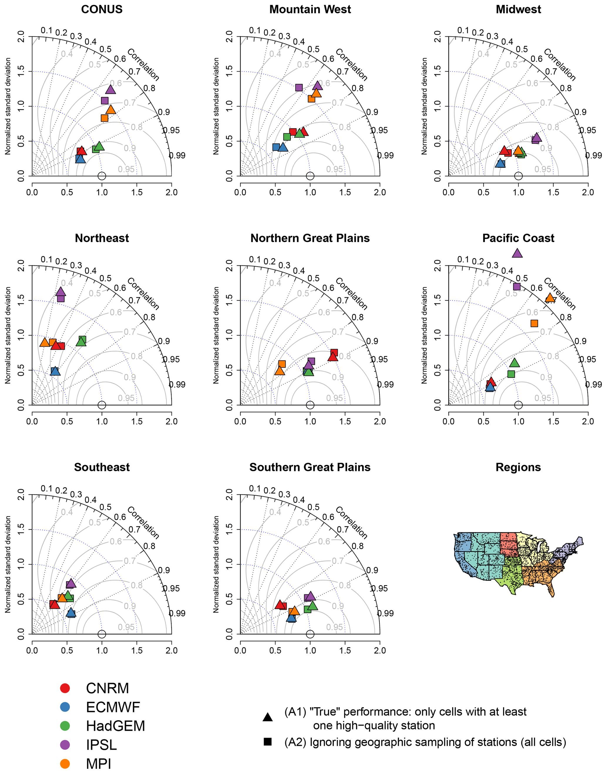
Figure 5Taylor diagrams comparing 20-year return values for CONUS and the climate subregions for the climate models versus regridded L15. The gray curvilinear lines represent the skill score for each model relative to the regridded L15.
Now considering the Taylor diagrams in Fig. 5, the effect of geographic sampling is generally smaller for larger spatial regions relative to the results for Utah in Fig. 3. The effect is particularly small for regions with dense geographic sampling like the Southeast, the Midwest, the Southern Great Plains, and Northern Great Plains. However, the most heterogeneous regions (the Mountain West and Pacific Coast) show the largest effects of sampling, even though as previously mentioned the geographic sampling is relatively good in the Pacific Coast. As with the extreme bias, when it makes a difference the effect of sampling is not the same across the models or these two climate regions. For example, in the Mountain West, there are some models that are more overdispersed (i.e., have too much spatial variability) relative to ignoring sampling (e.g., MPI), while in other cases the true ratio of variability is closer to 1 when accounting for geographic sampling (e.g., HadGEM). The spatial pattern correlation in the Mountain West is generally higher for approach A1, and the true performance of each model generally has a larger skill score relative to A2. In other words, if geographic sampling is ignored, one would conclude that the models are worse than they really are. Turning to the Pacific Coast region, when geographic sampling has a large effect (for HadGEM, IPSL, and MPI), the true performance of the model generally involves more spatial variability and smaller spatial pattern correlation relative to approach A2. However, in the Pacific Coast, the skill scores are generally higher for A2 than A1: for this region, ignoring geographic sampling leads one to conclude that the skills of the models are better than they actually are.
In summary, as with the case study in Sect. 4.1, our main point is that the sampling methodology is most important for regions that are highly heterogeneous. Particularly for the extreme bias, the choice of approach A1 vs. A2 can have a large effect regardless of sampling density, but the well-sampled regions generally show little change in the Taylor diagram metrics. Again, the specific effect of ignoring geographic sampling is not systematic in that the extreme bias, spatial variability, and spatial pattern correlation are impacted in different ways across the various models and climate regions considered.
In this paper, we have highlighted an important issue in comparing extremes from climate model output with observational data; namely, that it is important to account for the geographic sampling of weather station data. Our analysis of 5 d maxima demonstrates that while accounting for geographic sampling does not systematically change the performance of the models (in terms of bias, spatial pattern correlation, or standard deviation), one should nonetheless account for the sampling in order to yield a more appropriate comparison between models and observations. While our focus in this paper has been on 5 d maxima, we expect that similar results would hold for extreme daily or subdaily precipitation and possibly also the mean precipitation climatology. The integrated metrics considered in this paper (namely, extreme bias and Taylor diagrams) are helpful for gaining an overall sense of the model's ability to characterize the extreme climatology, but at the end of the day the quality of the local performance at high resolutions may be much different than what is suggested by, for example, a spatially averaged bias.
The analysis in this paper was motivated by the evaluation of high-resolution global climate models, by which we mean models with a 50 km horizontal resolution or finer. Multidecadal runs of such models are just now becoming widely available, even at the global scale, although the majority of modern global models generally have a coarser resolution. Accounting for the geographic sampling of weather stations using the criteria outlined in this paper (i.e., only considering grid cells with at least one high-quality station measurement) can have a larger effect as the horizontal resolution increases since many more grid cells will be excluded for a fixed network of high-quality stations. For example, across all of CONUS, the ∼20 km HadGEM model has a high-quality station in just 22 % of its grid cells, while the coarser ∼50 km IPSL model has a station in over 60 % of its grid cells. As previously mentioned, accounting for sampling as in this paper would have made no difference at all for a ∼300 km model like CanESM5 (see Fig. A1), which has at least one high-quality station in all of its CONUS grid cells. Of course, for lower-resolution models like CanESM5 it might be necessary to require a larger number of high-quality stations per grid cell.
In this paper, we have demonstrated that geographic sampling can make a difference with respect to model evaluation, but we do not suppose it is a perfect solution. Indeed, one of our primary motivations is the idea that a comparison of the climate model versus a gridded product over an area with poor observational sampling could be misleading, since the gridded product does not represent actual measurements of daily precipitation at these locations. However, it must also be admitted that a model quantity at the grid scale is considered a spatial average over subgrid scales, which offers an equally poor characterization of local values of the variable of interest in topographically complex regions. At the end of the day, a true like-for-like comparison is not possible: regardless of the method used to create a gridded data set, the scales of subgrid parameterizations are not the same as the scale of any station network. Thus, there is always a remaining mismatch. Even when one gets to convection-permitting models, the scale mismatch will remain. Our point in this paper is that accounting for the geographic sampling yields a more like-for-like comparison, even if mismatches remain.
In closing, it is important to note that our definitions of “well-sampled” and “poorly sampled” in this paper are all relative to the conterminous US, which is extremely well sampled overall relative to many other land regions. Nonetheless, we have demonstrated the importance of accounting for geographic sampling even for one of the most well-sampled parts of the globe. Sampling considerations will be even more important for the very poorly sampled parts of the world, e.g., Africa, South America, northern Asia, and the interior of Australia. The results for Kansas in our case study in Sect. 4.1 bode well for model evaluation in global regions that are poorly sampled but homogeneous in terms of either the climatology of extreme precipitation or orographic variability. However, it is not immediately obvious how the geographic sampling issue would translate for homogeneous regions that are climatologically very different from Kansas, e.g., desert regions like the interior of Australia or wet regions such as tropical rainforests.
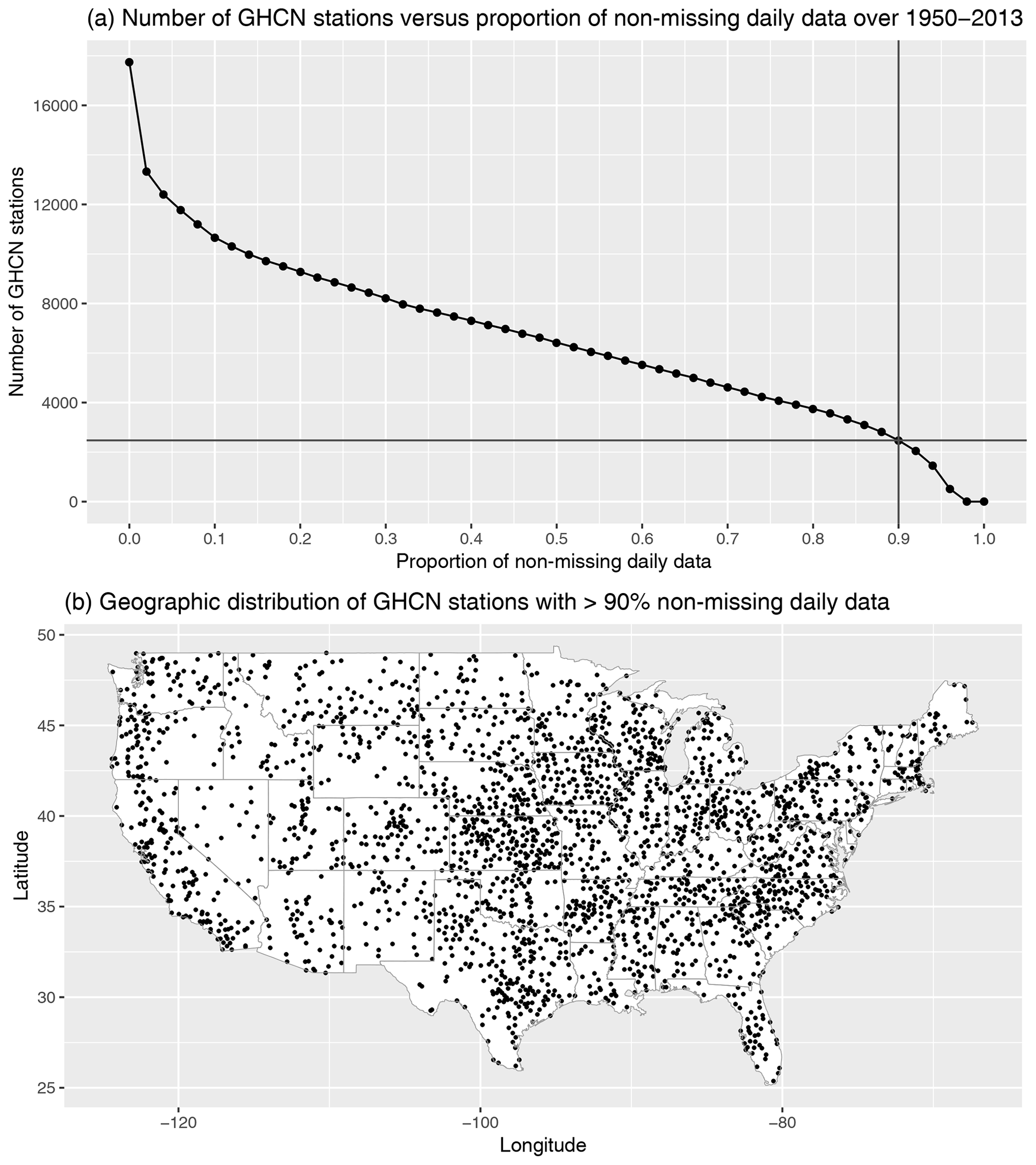
Figure A1The number of GHCN stations versus the proportion of non-missing daily data over 1950–2013 threshold, with the 90 % threshold used in this paper to define the n=2474 “high-quality” stations (a). The geographic distribution of the high-quality GHCN stations with at least 90 % of non-missing daily measurements over 1950–2013 (b).
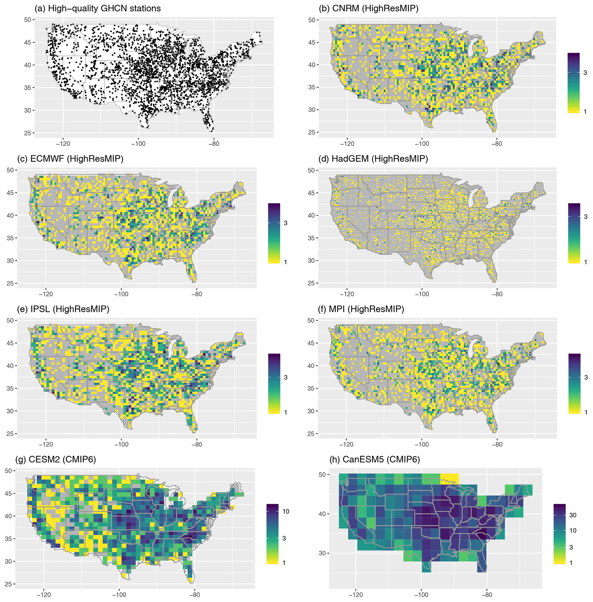
Figure A2The geographic distribution of the high-quality GHCN stations considered in the analysis (a), with the number of high-quality GHCN stations in each model grid cell for the HighResMIP models considered in this paper (b–f) and two CMIP6 models for comparison (g–h). Model grid cells without a representative high-quality GHCN station are shown in gray.
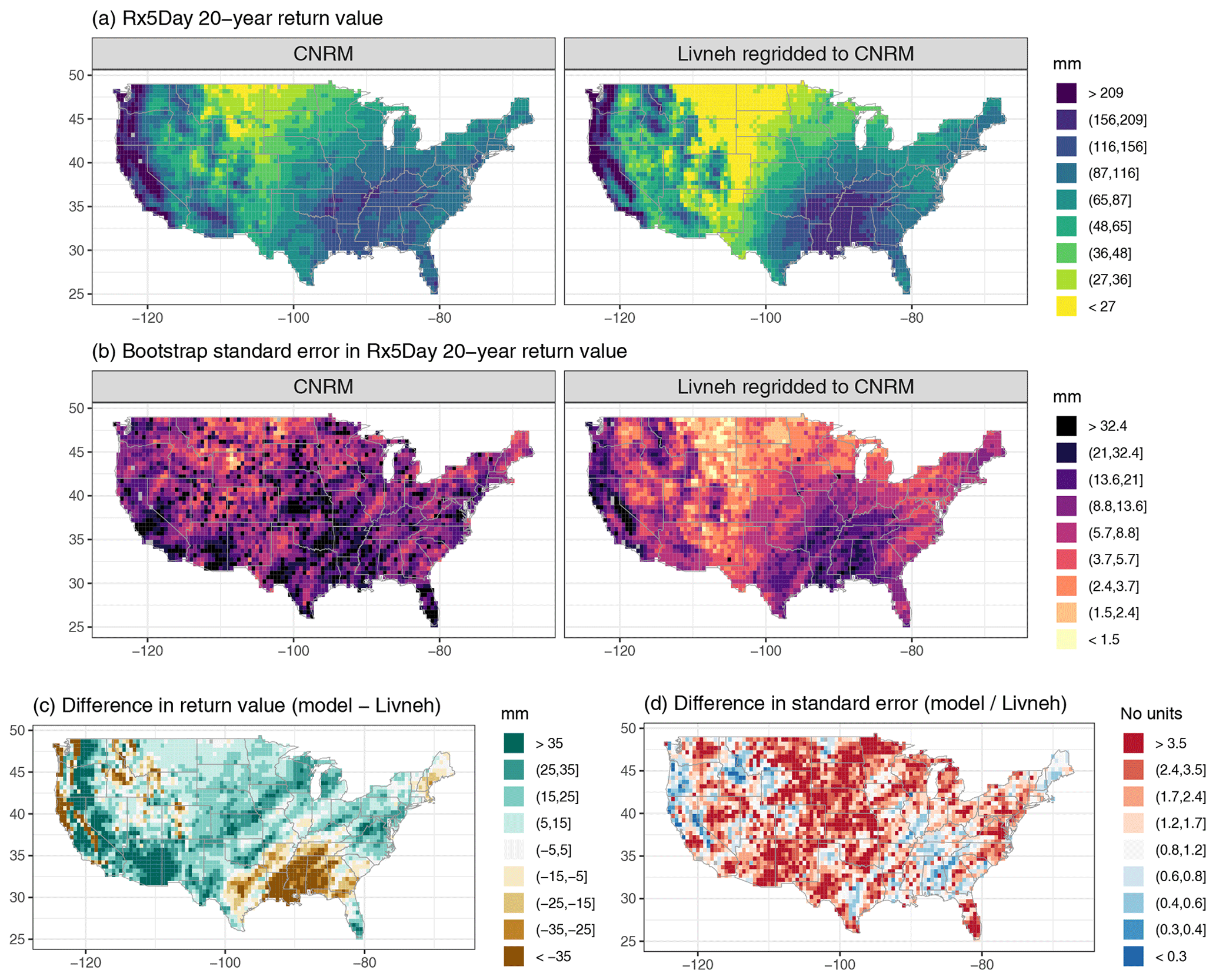
Figure A3Wintertime (DJF) 20-year return values in Rx5Day (mm) for the CNRM model and regridded L15 (a), with the bootstrap standard error (mm; b). Also shown is the difference in return values (model minus regridded L15) as well as the ratio of standard errors (model divided by regridded L15).
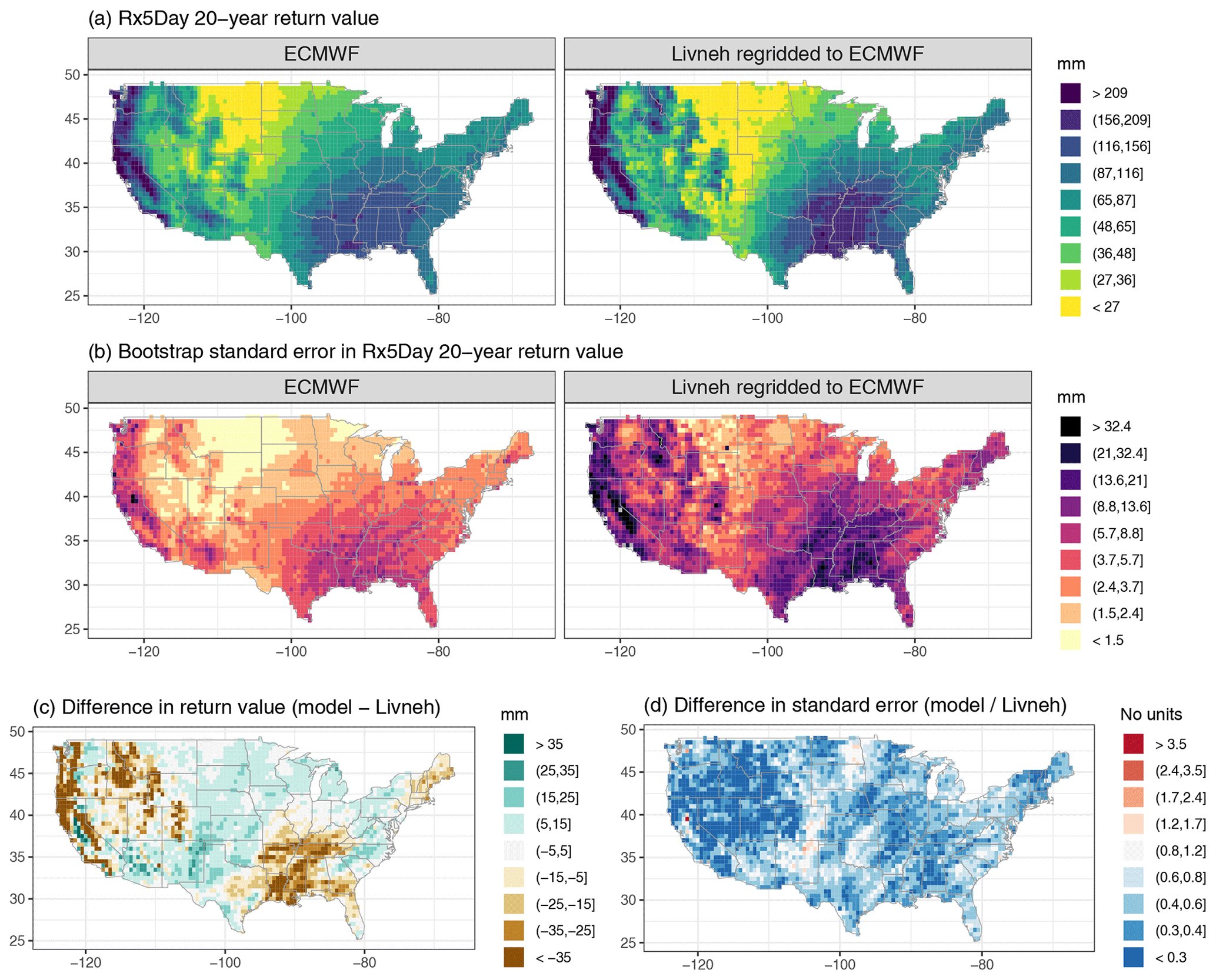
Figure A4Wintertime (DJF) 20-year return values in Rx5Day (mm) for the ECMWF model and regridded L15 (a), with the bootstrap standard error (mm; b). Also shown is the difference in return values (model minus regridded L15) as well as the ratio of standard errors (model divided by regridded L15).
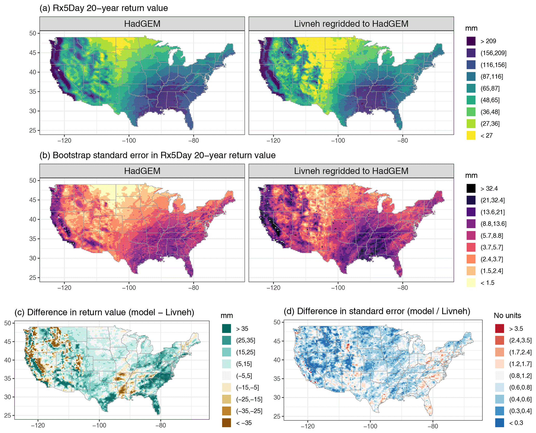
Figure A5Wintertime (DJF) 20-year return values in Rx5Day (mm) for the HadGEM model and regridded L15 (a), with the bootstrap standard error (mm; b). Also shown is the difference in return values (model minus regridded L15) as well as the ratio of standard errors (model divided by regridded L15).
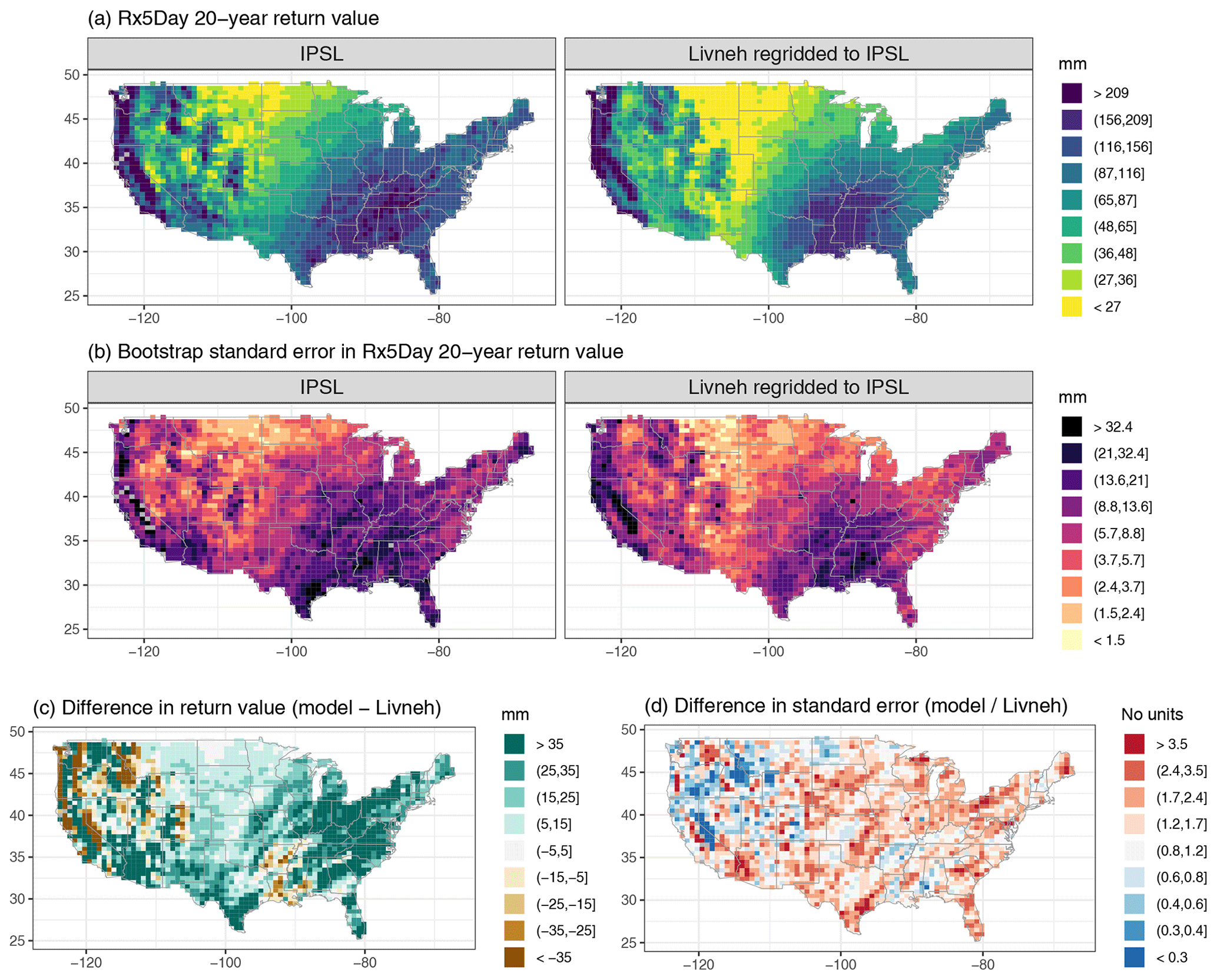
Figure A6Wintertime (DJF) 20-year return values in Rx5Day (mm) for the IPSL model and regridded L15 (a), with the bootstrap standard error (mm; b). Also shown is the difference in return values (model minus regridded L15) as well as the ratio of standard errors (model divided by regridded L15).

Figure A7Wintertime (DJF) 20-year return values in Rx5Day (mm) for the MPI model and regridded L15 (a), with the bootstrap standard error (mm; b). Also shown is the difference in return values (model minus regridded L15) as well as the ratio of standard errors (model divided by regridded L15).
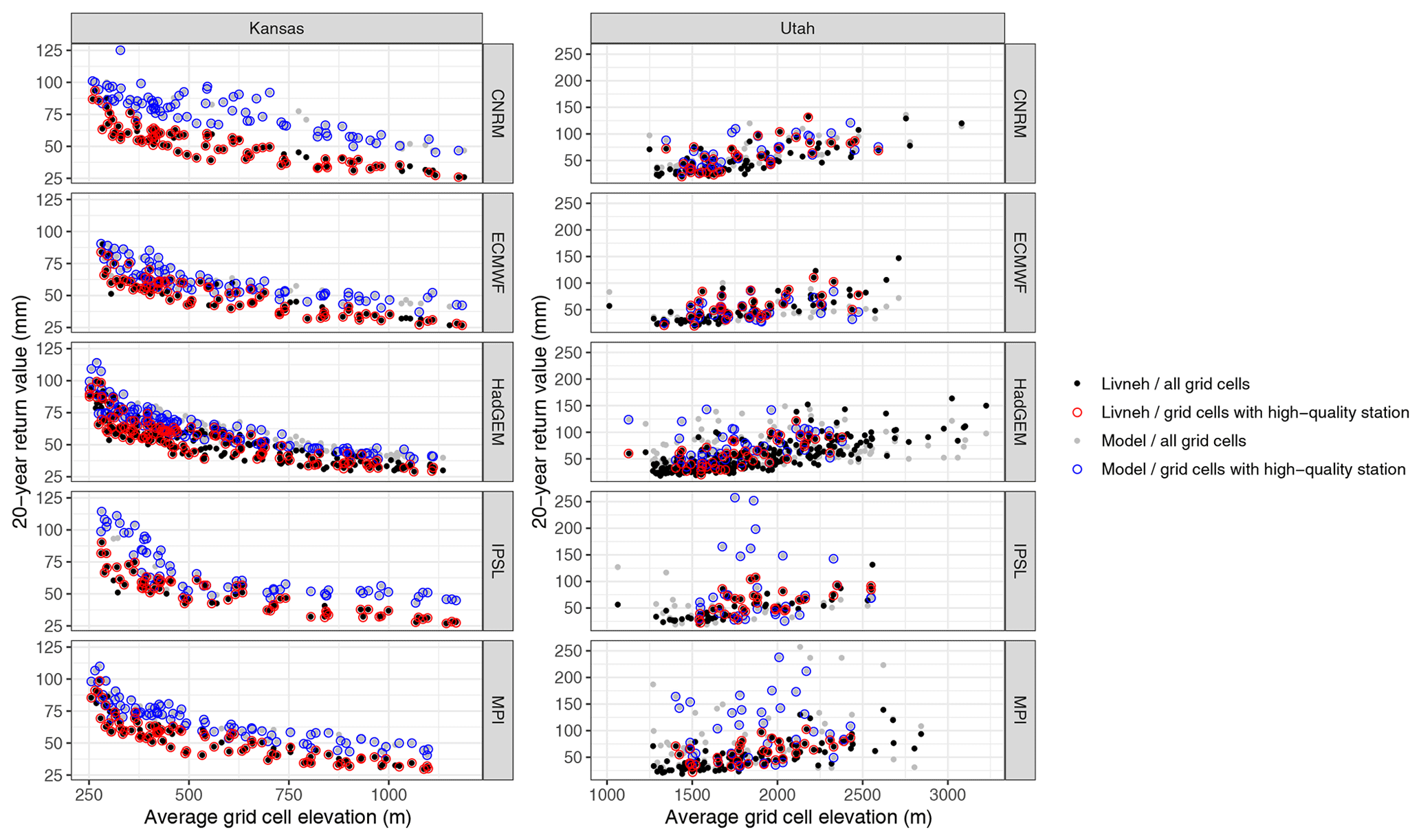
Figure A8The distribution of the grid cell average elevation (in meters; averaged from the GTOPO30 1 km digital elevation product) versus the Rx5Day 20-year return value (in millimeters) for Kansas and Utah across all model grids. Black dots represent the return values for all L15 grid cells, with gray dots representing the climate models. The colored circles (red for L15 and blue for the models) identify the grid cells that have at least one high-quality station and are used in the true model performance metrics.
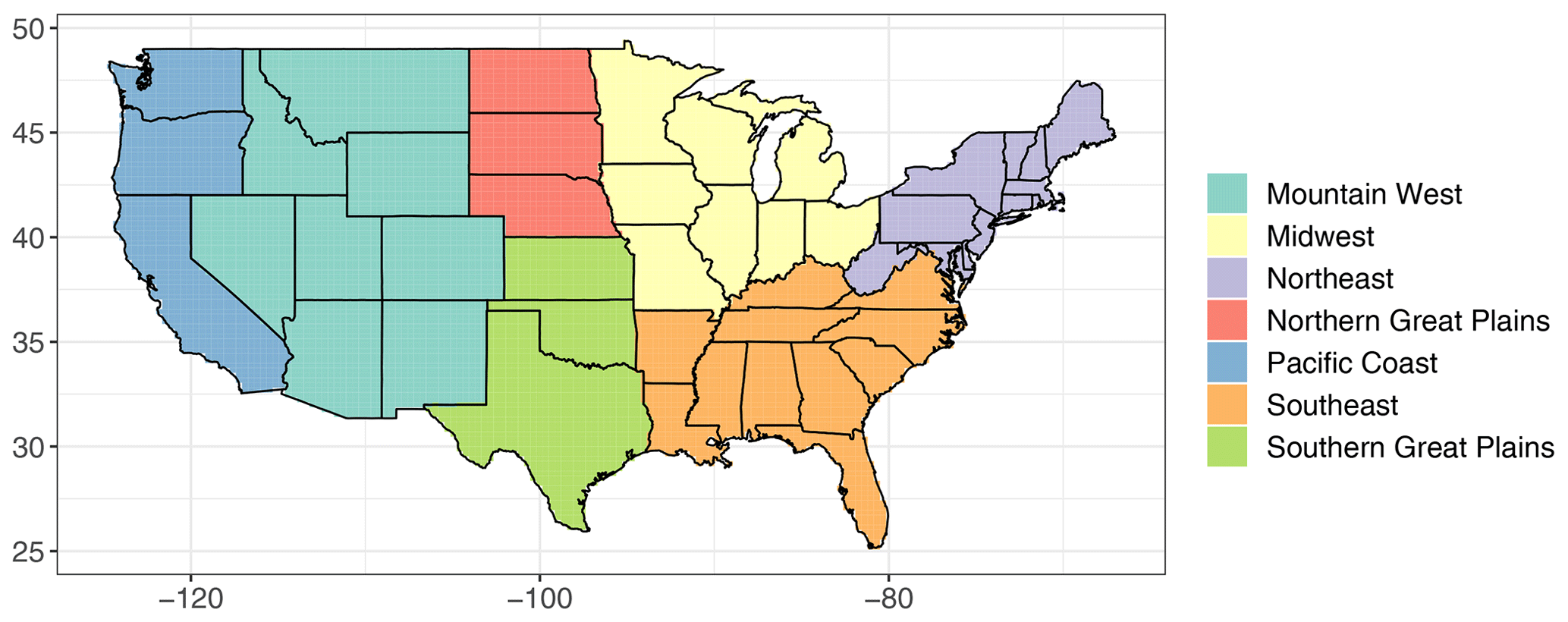
Figure A9The seven subregions used in our analysis. These are a slight variation on the regions defined in the Fourth National Climate Assessment.
Table A1Number of model grid cells in each study region (Nc), the number of model grid cells with at least one high-quality GHCN station (Nc+s), and the proportion of model grid cells with at least one high-quality GHCN station (Pc+s).
The observational data supporting this article are based on publicly available measurements from the National Centers for Environmental Information and https://data.nodc.noaa.gov/ncei/archive/data/0129374/daily/ (last access: 13 April 2020) for the L15 product. Model data were obtained for the IPSL and CNRM models from the Earth System Grid (https://esgf-node.llnl.gov/search/cmip6/, last access: 19 July 2019) and for the other models by early access to the Jasmin server in the UK. It is expected that all data used in this paper will eventually be uploaded to the CMIP6 data portals by the modeling groups themselves.
MFW and MDR contributed to developing methodological aspects of the paper. MFW contributed model data sets. MDR conducted all analyses. MDR and MFW contributed to the write-up of the article.
The authors declare that they have no conflict of interest.
This document was prepared as an account of work sponsored by the United States Government. While this document is believed to contain correct information, neither the United States Government nor any agency thereof, nor the Regents of the University of California, nor any of their employees, makes any warranty, express or implied, or assumes any legal responsibility for the accuracy, completeness, or usefulness of any information, apparatus, product, or process disclosed, or represents that its use would not infringe privately owned rights. Reference herein to any specific commercial product, process, or service by its trade name, trademark, manufacturer, or otherwise, does not necessarily constitute or imply its endorsement, recommendation, or favoring by the United States Government or any agency thereof, or the Regents of the University of California. The views and opinions of authors expressed herein do not necessarily state or reflect those of the United States Government or any agency thereof or the Regents of the University of California.
The authors would like to thank the associate editor and two anonymous reviewers and Charles Curry for their comments, which have greatly improved the quality of this manuscript.
This research was supported by the Office of Science, Office of Biological and Environmental Research, of the U.S. Department of Energy under contract no. DE-AC02-05CH11231 and used resources of the National Energy Research Scientific Computing Center (NERSC), also supported by the Office of Science of the U.S. Department of Energy, under contract no. DE-AC02-05CH11231.
This research has been supported by the Office of Science, Office of Biological and Environmental Research, of the U.S. Department of Energy (grant no. DE-AC02-05CH11231).
This paper was edited by Francis Zwiers and reviewed by Charles Curry and two anonymous referees.
Bacmeister, J. T., Hannay, C., Medeiros, B., Gettelman, A., Neale, R., Fredriksen, H. B., Lipscomb, W. H., Simpson, I., Bailey, D. A., Holland, M., and Lindsay, K.: CO2 increase experiments using the Community Earth System Model (CESM): Relationship to climate sensitivity and comparison of CESM1 to CESM2, J. Adv. Model Earth Sy., pp. 1850–2014, submitted, 2020. a
Boucher, O., Denvil, S., Caubel, A., and Foujols, M. A.: IPSL IPSL-CM6A-ATM-HR model output prepared for CMIP6 HighResMIP, Earth System Grid Federation, https://doi.org/10.22033/ESGF/CMIP6.2361, 2019. a
Chen, C.-T. and Knutson, T.: On the verification and comparison of extreme rainfall indices from climate models, J. Climate, 21, 1605–1621, 2008. a, b, c
Coles, S., Bawa, J., Trenner, L., and Dorazio, P.: An introduction to statistical modeling of extreme values, Lecture Notes in Control and Information Sciences, Springer, London, available at: https://books.google.com/books?id=2nugUEaKqFEC, 2001. a, b, c
Daly, C., Neilson, R. P., and Phillips, D. L.: A statistical-topographic model for mapping climatological precipitation over mountainous terrain, J. Appl. Meteorol., 33, 140–158, 1994. a
Daly, C., Halbleib, M., Smith, J. I., Gibson, W. P., Doggett, M. K., Taylor, G. H., Curtis, J., and Pasteris, P. P.: Physiographically sensitive mapping of climatological temperature and precipitation across the conterminous United States, Int. J. Climatol., 28, 2031–2064, 2008. a
Donat, M. G., Alexander, L. V., Yang, H., Durre, I., Vose, R., Dunn, R. J. H., Willett, K. M., Aguilar, E., Brunet, M., Caesar, J., and Hewitson, B.: Updated analyses of temperature and precipitation extreme indices since the beginning of the twentieth century: The HadEX2 dataset, J. Geophys. Res.-Atmos., 118, 2098–2118, 2013. a
Easterling, D., Kunkel, K., Arnold, J., Knutson, T., LeGrande, A., Leung, L., Vose, R., Waliser, D., and Wehner, M.: Precipitation change in the United States, in: Climate Science Special Report: Fourth National Climate Assessment, Volume I, pp. 207–230, https://doi.org/10.7930/J0H993CC, 2017. a
Fischer, E. M. and Knutti, R.: Anthropogenic contribution to global occurrence of heavy-precipitation and high-temperature extremes, Nat. Clim. Change, 5, 560, 2015. a
Gervais, M., Tremblay, L. B., Gyakum, J. R., and Atallah, E.: Representing extremes in a daily gridded precipitation analysis over the United States: Impacts of station density, resolution, and gridding methods, J. Climate, 27, 5201–5218, 2014. a, b, c, d, e, f, g
GISTEMP Team: GISS Surface Temperature Analysis (GISTEMP), version 4, NASA Goddard Institute for Space Studies, dataset, https://data.giss.nasa.gov/gistemp/data, last access: 14 April 2020. a
Gutjahr, O., Putrasahan, D., Lohmann, K., Jungclaus, J. H., von Storch, J.-S., Brüggemann, N., Haak, H., and Stössel, A.: Max Planck Institute Earth System Model (MPI-ESM1.2) for the High-Resolution Model Intercomparison Project (HighResMIP), Geosci. Model Dev., 12, 3241–3281, https://doi.org/10.5194/gmd-12-3241-2019, 2019. a
Haarsma, R. J., Roberts, M. J., Vidale, P. L., Senior, C. A., Bellucci, A., Bao, Q., Chang, P., Corti, S., Fučkar, N. S., Guemas, V., von Hardenberg, J., Hazeleger, W., Kodama, C., Koenigk, T., Leung, L. R., Lu, J., Luo, J.-J., Mao, J., Mizielinski, M. S., Mizuta, R., Nobre, P., Satoh, M., Scoccimarro, E., Semmler, T., Small, J., and von Storch, J.-S.: High Resolution Model Intercomparison Project (HighResMIP v1.0) for CMIP6, Geosci. Model Dev., 9, 4185–4208, https://doi.org/10.5194/gmd-9-4185-2016, 2016. a, b, c
Jones, P., Osborn, T., Briffa, K., Folland, C., Horton, E., Alexander, L., Parker, D., and Rayner, N.: Adjusting for sampling density in grid box land and ocean surface temperature time series, J. Geophys. Res. - Atmos., 106, 3371–3380, 2001. a
Jones, P. W.: First-and second-order conservative remapping schemes for grids in spherical coordinates, Mon. Weather Rev., 127, 2204–2210, 1999. a
King, A. D., Alexander, L. V., and Donat, M. G.: The efficacy of using gridded data to examine extreme rainfall characteristics: a case study for Australia, Int. J. Climatol., 33, 2376–2387, 2013. a
Kunkel, K. E.: North American trends in extreme precipitation, Nat. Hazards, 29, 291–305, 2003. a
Lenssen, N. J., Schmidt, G. A., Hansen, J. E., Menne, M. J., Persin, A., Ruedy, R., and Zyss, D.: Improvements in the GISTEMP uncertainty model, J. Geophys. Res. - Atmos., 124, 6307–6326, 2019. a
Li, C., Zwiers, F., Zhang, X., and Li, G.: How much information is required to well constrain local estimates of future precipitation extremes? Earth's Future, 7, 11–24, 2019. a
Livneh, B., Bohn, T. J., Pierce, D. W., Munoz-Arriola, F., Nijssen, B., Vose, R., Cayan, D. R., and Brekke, L.: A spatially comprehensive, hydrometeorological data set for Mexico, the US, and Southern Canada (NCEI Accession 0129374), NOAA National Centers for Environmental Information, Dataset, (Daily precipitation), https://doi.org/10.7289/v5x34vf6 (last access: 13 April 2020), 2015a. a
Livneh, B., Bohn, T. J., Pierce, D. W., Munoz-Arriola, F., Nijssen, B., Vose, R., Cayan, D. R., and Brekke, L.: A spatially comprehensive, hydrometeorological data set for Mexico, the US, and Southern Canada 1950–2013, Scientific data, 2, 1–12, 2015b. a, b, c
Lovejoy, S., Schertzer, D., and Allaire, V.: The remarkable wide range spatial scaling of TRMM precipitation, Atmos. Res., 90, 10–32, https://doi.org/10.1016/j.atmosres.2008.02.016, available at: http://linkinghub.elsevier.com/retrieve/pii/S0169809508000562, 2008. a
Madden, R. A. and Meehl, G. A.: Bias in the global mean temperature estimated from sampling a greenhouse warming pattern with the current surface observing network, J. Climate, 6, 2486–2489, 1993. a
Maskey, M. L., Puente, C. E., Sivakumar, B., and Cortis, A.: Encoding daily rainfall records via adaptations of the fractal multifractal method, Stochastic Environmental Research and Risk Assessment, 30, 1917–1931, https://doi.org/10.1007/s00477-015-1201-7, available at: http://link.springer.com/10.1007/s00477-015-1201-7, 2016. a
Menne, M. J., Durre, I., Vose, R. S., Gleason, B. E., and Houston, T. G.: An overview of the Global Historical Climatology Network-Daily database, Journal of Atmospheric and Oceanic Technology, 29, 897–910, 2012. a, b
Min, S.-K., Zhang, X., Zwiers, F. W., and Hegerl, G. C.: Human contribution to more-intense precipitation extremes, Nature, 470, 378, 2011. a
Paciorek, C.: climextRemes: Tools for Analyzing Climate Extremes, https://CRAN.R-project.org/package=climextRemes (last access: 1 January 2019), R package version 2.1, 2016. a
Risser, M. D. and Wehner, M. F.: Attributable Human-Induced Changes in the Likelihood and Magnitude of the Observed Extreme Precipitation during Hurricane Harvey, Geophys. Res. Lett., 44, 12,457–12,464, https://doi.org/10.1002/2017GL075888, available at: https://agupubs.onlinelibrary.wiley.com/doi/abs/10.1002/2017GL075888, 2017. a
Risser, M. D., Paciorek, C. J., O'Brien, T. A., Wehner, M. F., and Collins, W. D.: Detected Changes in Precipitation Extremes at Their Native Scales Derived from In Situ Measurements, J. Climate, 32, 8087–8109, https://doi.org/10.1175/JCLI-D-19-0077.1, 2019a. a, b, c
Risser, M. D., Paciorek, C. J., Wehner, M. F., O'Brien, T. A., and Collins, W. D.: A probabilistic gridded product for daily precipitation extremes over the United States, Clim. Dynam., 53, 2517–2538, https://doi.org/10.1007/s00382-019-04636-0, 2019b. a, b, c
Roberts, C. D., Senan, R., Molteni, F., Boussetta, S., Mayer, M., and Keeley, S. P. E.: Climate model configurations of the ECMWF Integrated Forecasting System (ECMWF-IFS cycle 43r1) for HighResMIP, Geosci. Model Dev., 11, 3681–3712, https://doi.org/10.5194/gmd-11-3681-2018, 2018. a
Roberts, M. J., Baker, A., Blockley, E. W., Calvert, D., Coward, A., Hewitt, H. T., Jackson, L. C., Kuhlbrodt, T., Mathiot, P., Roberts, C. D., Schiemann, R., Seddon, J., Vannière, B., and Vidale, P. L.: Description of the resolution hierarchy of the global coupled HadGEM3-GC3.1 model as used in CMIP6 HighResMIP experiments, Geosci. Model Dev., 12, 4999–5028, https://doi.org/10.5194/gmd-12-4999-2019, 2019. a, b
Swart, N. C., Cole, J. N. S., Kharin, V. V., Lazare, M., Scinocca, J. F., Gillett, N. P., Anstey, J., Arora, V., Christian, J. R., Hanna, S., Jiao, Y., Lee, W. G., Majaess, F., Saenko, O. A., Seiler, C., Seinen, C., Shao, A., Sigmond, M., Solheim, L., von Salzen, K., Yang, D., and Winter, B.: The Canadian Earth System Model version 5 (CanESM5.0.3), Geosci. Model Dev., 12, 4823–4873, https://doi.org/10.5194/gmd-12-4823-2019, 2019. a
Taylor, K. E.: Summarizing multiple aspects of model performance in a single diagram, J. Geophys. Res. - Atmos., 106, 7183–7192, 2001. a, b, c
Timmermans, B., Wehner, M., Cooley, D., O'Brien, T., and Krishnan, H.: An evaluation of the consistency of extremes in gridded precipitation data sets, Clim. Dynam., 52, 6651–6670, https://doi.org/10.1007/s00382-018-4537-0, 2019. a
Voldoire, A., Sanchez-Gomez, E., Salas y Mélia, D., Decharme, B., Cassou, C., Sénési, S., Valcke, S., Beau, I., Alias, A., Chevallier, M., Déqué, M., Deshayes, J., Douville, H., Fernandez, E., Madec, G., Maisonnave, E., Moine, M.-P., Planton, S., Saint-Martin, D., Szopa, S., Tyteca, S., Alkama, R., Belamari, S., Braun, A., Coquart, L., and Chauvin, F.: The CNRM-CM5.1 global climate model: description and basic evaluation, Clim. Dynam., 40, 2091–2121, https://doi.org/10.1007/s00382-011-1259-y, 2013. a
von Hardenberg, J.: rainfarmr: Stochastic Precipitation Downscaling with the RainFARM Method, https://CRAN.R-project.org/package=rainfarmr (last access: 13 April 2020), R package version 0.1, 2019. a
Vose, R. S., Wuertz, D., Peterson, T. C., and Jones, P.: An intercomparison of trends in surface air temperature analyses at the global, hemispheric, and grid-box scale, Geophys. Res. Lett., 32, 2005. a
Wehner, M. F.: Very extreme seasonal precipitation in the NARCCAP ensemble: model performance and projections, Clim. Dynam., 40, 59–80, 2013. a
Wuebbles, D. J., Fahey, D. W., and Hibbard, K. A.: Climate science special report, fourth National Climate Assessment, volume I, 2017. a
Zhang, X., Wan, H., Zwiers, F. W., Hegerl, G. C., and Min, S.-K.: Attributing intensification of precipitation extremes to human influence, Geophysical Research Letters, 40, 5252–5257, 2013. a