Using wavelets to verify the scale structure of precipitation forecasts

Recently developed verification tools based on local wavelet spectra can isolate errors in the spatial structure of quantitative precipitation forecasts, thereby answering the question of whether the predicted rainfall variability is distributed correctly across a range of spatial scales. This study applies the wavelet-based structure scores to real numerical weather predictions and radar-derived observations for the first time. After tackling important practical concerns such as uncertain boundary conditions and missing data, the behaviour of the scores under realistic conditions is tested in selected case studies and analysed systematically across a large data set. Among the two tested wavelet scores, the approach based on the so-called map of central scales emerges as a particularly convenient and useful tool: summarizing the local spectrum at each pixel by its centre of mass results in a compact and informative visualization of the entire wavelet analysis. The histogram of these scales leads to a structure score which is straightforward to interpret and insensitive to free parameters like wavelet choice and boundary conditions. Its judgement is largely the same as that of the alternative approach (based on the spatial mean wavelet spectrum) and broadly consistent with other, established structural scores.

1 Introduction

The quantitative prediction of precipitation is a central task of modern weather forecasting. A demand for improved predictions of localized severe rainfall events, in particular, has been one of the main drivers behind the development of forecast models with increasingly fine resolutions (Baldauf et al., 2011; Seity et al., 2011), sophisticated parametrizations (Seifert and Beheng, 2006; Kuell and Bott, 2008) and assimilation of novel observation data (Stephan et al., 2008; Bick et al., 2016).

Whether or not the desired improvement has actually been achieved, however, is no trivial question. Since rain fields are inherently intermittent in space and time, a pixel-wise forecast verification can only reward the correct intensity, shape and structure of predicted rain patterns if their locations match exactly with the observed ones. Even a slight displacement between forecast and observation results in a double penalty, because the forecast is wrong in both the observed and the predicted location. The naive, grid-point-wise approach will generally favour coarse models over highly resolved ones and can neither assess the structure or intensity of displaced rain objects nor appropriately judge the severity of displacement errors. Recent years have seen the development of numerous so-called spatial verification techniques, which address the double penalty problem in a variety of ways (Gilleland et al., 2009; Dorninger et al., 2018).One strategy espoused by many of these techniques is to split the total forecast error into a number of (ideally orthogonal) components, thereby separating, for example, displacement from other kinds of errors. Following this idea, the present study uses a shift-invariant wavelet transform (Eckley et al., 2010) to isolate a single aspect of forecast performance, namely its structure. Our method, first introduced in Buschow et al. (2019), transforms a map of rain intensities into local wavelet spectra that measure the energy (variance) of the rain field for each combination of location and spatial scale. Under the assumption that auto-correlations vary only slowly in space, the connection between wavelet spectra and the spatial covariance function can be formalized via the theory of locally stationary wavelet processes (Eckley et al., 2010). In order to compare forecast and observation, we can either average the local spectra in space to obtain mean spectra, or calculate the dominant scale at each location and then evaluate the histograms of these central scales. Using a physics-based stochastic rain model (Hewer, 2018) as a controlled test bed, Buschow et al. (2019) have demonstrated that both approaches lead to double-penalty free verification procedures which can detect discrepancies between the observed and predicted correlation structure with great accuracy.

In the present study, we apply the wavelet-based structure scores of Buschow et al. (2019) to real numerical weather forecasts, focusing on the verification of deterministic predictions. Besides addressing some of the practical challenges associated with the non-idealized setting (boundary conditions, missing data, treatment of extremes), one main goal is to study which kinds of errors are typically evaluated by our method. Apart from the consideration of selected case studies, it is therefore instructive to compare the new approach to established alternatives from the rich literature of verification techniques.

Although the standard taxonomy of spatial verification techniques (Dorninger et al., 2018) classifies our method as a scale-separation approach, this class does not actually contain many useful objects of comparison. The most popular approach (Casati et al., 2004, ISS), while also relying on wavelets, studies the scale of the error, whereas our method assesses the error of the scales. The ISS therefore does not separate structure from displacement and is no direct “competitor” of our approach. Yano and Jakubiak (2016) employ a different type of wavelet transform to locate dominant features in space and scale before explicitly measuring their displacement error. Lastly Kapp et al. (2018), who developed the direct precursor to our method and employ the same wavelet transform, only consider ensemble forecasts and do not separate correlation structure from total variance. For our purposes, it is thus more helpful to group verification methods by the forecast attributes they aim to assess. In this way, we can identify the object-based structure error S of (Wernli et al., 2008) and the variogram-based scoring rules developed by Scheuerer and Hamill (2015) as two comparable pure structure scores.

To obtain robust results on the merits and interrelationship of the object-, variogram- and wavelet-based structure verification, we consider a large set of highly resolved forecasts from the COSMO-DE ensemble prediction system (COSMO-DE-EPS). The hourly adjusted radar product RADOLAN, as well as the regional reanalysis COSMO-REA2 (Wahl et al., 2017), serve as our reference fields. Although we verify each member of COSMO-DE-EPS individually, the ensemble nature of this data set is nonetheless very useful for our purposes. Besides giving us a great number of individual predictions (20 forecasts on 127 selected days), we can exploit the fact that each ensemble prediction consists of 20 realizations from a distribution which changes from case to case to set up idealized experiments: presented with a single member from one of the 127 ensembles, can our scores find the other 19 fields based on their similar correlation structure alone?

The remainder of this paper begins, in Sect. 2, with an overview of all relevant data sets. Section 3 details all steps related to the wavelet transform and its spatial aggregation. To get the first overview of the results of this transform, we analyse the climatology of observed and predicted spectra in Sect. 4. The wavelet-based structure scores of Buschow et al. (2019) are introduced and applied to two selected case studies in Sect. 5. Section 6 reviews the alternative scores from the literature before the verification of the full COSMO-DE-EPS data set in Sect. 7. Here, we study the relationship between all structure scores (Sect. 7.1), assess their discriminatory abilities (Sect. 7.2) and test the sensitivity of our wavelet scores to the free parameters of the method (Sect. 7.3). The paper concludes with a discussion and outlook in Sect. 8.

2 Data

As mentioned in the introduction, this study relies on COSMO-DE-EPS forecasts and COSMO-REA2 reanalysis data (Wahl et al., 2017, henceforth REA2), both of which were previously considered by Kapp et al. (2018). The COSMO-DE ensemble prediction system (Peralta et al., 2012), which has been operational at DWD since May 2012, is based on the non-hydrostatic regional NWP-model COSMO (Baldauf et al., 2011), run at a convection-permitting resolution of 2.8 km in a domain covering Germany and parts of all neighbouring countries (dashed lines in Fig. 1). The 20 ensemble members are generated by combining four boundary conditions with five slightly perturbed physics parametrizations.

The regional reanalysis REA2 is based on a similar version of COSMO, albeit run on a slightly larger domain (white mask in Fig. 1) and at finer resolution of 2 km. As in Kapp et al. (2018), the slight difference in grid is resolved via simple nearest neighbour interpolation to the coarser grid. We have checked that the choice of interpolation scheme has very little impact on the results of our verification procedure. The reanalysis contains information from conventional observations, assimilated in a continuous nudging scheme, as well as radar observations which were included via latent heat nudging. The latter point in particular makes REA2 an attractive validation data set for our purposes since it encompasses direct measurements of rainfall while avoiding systematic discrepancies with the model due to measurement errors or spatial interpolation schemes.

Highly resolved regional reanalyses, while clearly convenient, are not available in most parts of the world and may also contain the same biases as the numerical models verified against them. It is thus of great interest to know whether our methodology can also be applied to direct observational data. In this study, we therefore use DWD's hourly RADOLAN-RW (Winterrath et al., 2018) product as our main validation data set. Rain gauge adjusted radar products such as RADOLAN are more widely available and additionally allow us to verify both model and reanalysis against more direct observation data which is completely independent from any dynamical model. Kapp et al. (2018) did not use radar data in order to avoid issues with missing data. This study will explore how big such effects actually are. As for REA2, we bridge the slight difference in nominal resolution (RADOLAN being available at 1 km×1 km) via nearest neighbour interpolation to the COSMO-DE-EPS grid. Due to the adjustment with rain gauge data, the RADOLAN-RW product is cropped to roughly the German national borders (dotted line in Fig. 1). For the purposes of verification, values outside of the RADOLAN domain, as well as the occasional missing values within, are set to zero. To ensure a fair comparison, the same pixels are set to zero in the forecast and reanalysis fields as well.

Forecasts of hourly rain sums were provided by DWD for the complete year 2011. Since our focus is on an evaluation of the rain field's texture, it stands to reason that the total rain area has to reach some minimum extent since very small rain objects leave us with too few data to confidently estimate the spatial correlations. In this study, we therefore select only cases where at least 5 % of the pixels in the RADOLAN-field have non-zero rain. We furthermore consider only the afternoon hours (16:00–19:00 UTC) in order to ensure comparable lead times. For each day which meets our criteria, we select the hour with the greatest total rain area. This selection procedure leaves us with 127 cases for which the ensemble issues a total of 2540 individual predictions.

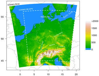
Figure 1 Domain and model orography of COSMO-REA2 in metres. Dashed lines delineate the COSMO-DE-EPS domain, and the dotted line corresponds to the maximum extent of the RADOLAN-RW data set used in this study.

In order to roughly classify the 127 case studies according to the processes which generate precipitation, we have manually checked the corresponding DWD analysis maps (freely available from http://www1.wetter3.de/, last access: February 2020) and the registered lightning events (observed by the community project http://www.lightningmaps.org, last access: February 2020). For each day, we note the occurrence of cold fronts, warm fronts, other fronts (quasi-stationary and occlusion fronts), convergence lines and deep moist convection (observed lightning being a proxy for the latter) in the domain. The auxiliary data set is summarized in Fig. 2. We observe that the majority of notable afternoon precipitation episodes in 2011 was associated with lightning (indicating convective processes), often in combination with occlusion or quasi-stationary fronts. The considered time span is furthermore long enough to contain several examples of both purely frontal and purely convective events.

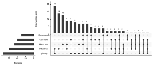
Figure 2 Frequency of weather events and their combinations during the 127 d considered. Data visualized using the UpSetR R package (Conway et al., 2017).

3 Estimation of local wavelet spectra

3.1 Redundant discrete wavelet transforms and local stationarity

Our first objective is to extract the structural properties of observed and predicted fields in a shift-invariant manner. This is achieved by projecting the data, given as a matrix M of dimension n_x×n_y, onto an overcomplete set of basis functions of the form ${\mathit{\psi }}_{j,d,u}\left(r\right)=s_j^{-\mathrm{1}/\mathrm{2}}{\mathit{\psi }}_d\left(\frac{r-u}{s_j}\right)$. These so-called daughter wavelets are obtained from their mother wavelet ψ(r) via a shift u, scaling s_j and change in orientation, here denoted by the index d. The redundant discrete wavelet transform (RDWT) is defined by scales which are whole powers of two (s_j=2^j, $j\in \mathit{\{}\mathrm{1},\mathrm{2},\mathrm{\dots },J\mathit{\}}$), includes three directions (d=1: vertical, d=2: horizontal, d=3: diagonal) and allows shifts to all locations on the grid of the data. The redundancy introduced in this manner ensures that this transformation is shift invariant in the sense that a shift of the input field merely leads to a shift of the coefficient fields. Without this property, the outcome of the verification would depend on the absolute location of rain features within the domain. One basic requirement of the transformation is that the dimensions of M are exactly $n_x=n_y={\mathrm{2}}^J$ – we discuss solutions to this boundary problem in some detail in Sect. 3.3.

At this point, we face two natural questions: how are the wavelet coefficients related to the structure of the underlying field, i.e., its spatial covariance matrix, and how should we deal with the great redundancy of the transformed field? Both of these issues can be resolved by assuming that our data are generated by a locally stationary two-dimensional wavelet process (henceforth LS2W). This two-dimensional stochastic process introduced by Eckley et al. (2010) is defined as

$$\begin{array}{}\text{(1)}& X\left(r\right)=\sum _{j=\mathrm{1}}^J\sum _{d=\mathrm{1}}^{\mathrm{3}}\sum _{\text{all }u}{W}_{j,d,u}{\mathit{\psi }}_{j,d,u}\left(r\right){\mathit{\xi }}_{j,d,u},\end{array}$$

where the $W_{j,d,u}$ represent fixed weights associated with each daughter wavelet and ${\mathit{\xi }}_{j,d,u}$ is a random white-noise increment. We assume that the spatial covariance of X varies only slowly with r. This requirement of local stationarity is weaker than global stationarity and can be formalized as constraints on the regularity of $W_{j,d,u}$ (Eckley et al., 2010). If local stationarity holds, it can be shown that the spatial autocovariances of X in the limit of an infinitely large domain are completely determined by, and can be inferred from, the set of all $|W_{j,d,u}{|}^{\mathrm{2}}$. Moreover, the squared wavelet coefficient corresponding to ${\mathit{\psi }}_{j,d,u}\left(r\right)$ is a biased estimator of $|W_{j,d,u}{|}^{\mathrm{2}}$. The bias, which mostly consists of an over-emphasis on the very large scales, can be removed by multiplication with a wavelet-specific matrix $A_{\mathit{\psi }}^{-\mathrm{1}}$. In analogy to the Fourier spectrum, the 3×J bias-corrected squared coefficients at each grid point are called the local wavelet spectrum. Since any practical application falls outside the realm of asymptotic limits, the bias correction is only approximate, occasionally overshoots its target and introduces negative values to the local spectra. We will set such values, which have no useful interpretation as “energy”, to zero before proceeding with our verification.

Figure 3 Vertical (a), horizontal (b) and diagonal (c) daughter wavelet for D₂.

The need for a bias correction limits our choice of mother wavelet ψ to the Daubechies family (Daubechies, 1992) for which Eckley et al. (2010) derived the corresponding matrices $A_{\mathit{\psi }}^{-\mathrm{1}}$. We refer to the compactly supported Daubechies wavelets as D_n. Intuitively, large values of the index n∈ℕ correspond to smooth functions with good localization in frequency, whereas small n means good localization in space, i.e., a small support size.

Table 1 Side length of the daughter wavelets' support as a function of the scale j for the first 10 Daubechies wavelets. For each mother wavelet, the star marks the largest daughter wavelet with support size smaller than 2⁹.

The support sizes of the first four Daubechies daughter wavelets are listed in Table 1. A daughter with support size greater than 2^J is no longer unambiguously localized since it “wraps around” the domain more than once (some grid points are sampled multiple times due to the cyclic convolutions of the transform). To avoid this effect, we truncate the local spectra at the largest scale that fits inside the domain. In order to avoid spreading the information from these untrustworthy daughters to the rest of the spectrum (and incidentally spreading information from the uncertain boundaries), scales that are too large are removed prior to bias correction.

For the model given by Eq. (1) to be appropriate, we select the D_n which is most similar to the data using the wavelet selection procedure of Goel and Vidakovic (1995). A few details concerning this step are given in Appendix A. For the present data set, D₂ emerges as the overall winner and is used for the rest of this investigation. Consequently, the largest used scale is j=7 (see Table 1). The three directional versions of D₂ are shown in Fig. 3. Observing their complicated structure, we recognize that the location within the support of ${\mathit{\psi }}_{j,d,u}$ to which the corresponding spectral value should be assigned is not obvious. As a heuristic solution, we simply select the centre of mass of ${\mathit{\psi }}_{j,d,u}^{\mathrm{2}}$. Features in the resulting local spectra are thus located close to the corresponding features in the input image.

Concluding this section, we note that our spectrum is not a consistent estimator of $|W_{j,d,u}{|}^{\mathrm{2}}$ (it has non-vanishing variance in the limit of infinite domain sizes), which necessitates a spatial smoothing of the wavelet coefficients (Eckley et al., 2010). Unless noted otherwise we will omit this step from our present investigation for several reasons: firstly, smoothing introduces a number of additional free parameters which are undesirable for a verification procedure. Secondly, information from the uncertain boundary regions (introduced by expanding the field to 2^J×2^J) is spread across the domain. Lastly, some smoothing algorithms can incur significant additional computational costs. Asymptotic inconsistency is therefore accepted as the cost of a more streamlined verification procedure.

3.2 Logarithmic transformation

Before applying the RDWT to our observed and predicted rain fields, we set all values below 0.1 mm to zero, 0.1 mm being the smallest non-zero value registered by RADOLAN. This step is generally advisable as it removes extremely low-intensity model noise which cannot be interpreted as an actual forecast of precipitation. Next, we replace the original rain fields by their binary logarithm. Casati et al. (2004) argue that this procedure corresponds to an approximate “normalization” of the data. Schleiss et al. (2014), who studied the non-stationary structure of rain fields, concur that this type of variance stabilization facilitates structural analysis.

Thinking visually, the log-transform can be interpreted as a change in colour scale: very few meteorological publications visualize precipitation on a linear scale since it frequently over-emphasizes small, intense showers while rendering the boundary between rain and no rain invisible. In fact, only 5 of the 46 figures depicting rain fields in publications cited in this paper or Buschow et al. (2019) have linear colour scales. The typical step-wise alternatives have many bins near zero and few bins at large values. It is easy to imagine situations where a human assessor will disagree with algorithmically calculated scores if the scores are based on the original data (linear colour scale) while the human is looking at transformed data. The conflict is resolved by basing both judgements on the logarithm of the fields: a logarithmic colour scale achieves a similar effect as the step-wise alternatives mentioned above and can easily be used as the input for our algorithm. This step furthermore dampens the potential impact of strongly localized extreme events on our evaluation: without such precaution, a single high-intensity rain object could overshadow the rest of the field, shifting the overall distribution of power to very small scales.

It should be noted that the logarithm introduces one additional free parameter, namely the new value assigned to pixels with zero rain. For this study, it will be set to ${\log }_{\mathrm{2}}\left(\mathrm{0.1}\right)\approx -\mathrm{3}$, i.e., the logarithm of the smallest considered non-zero intensity. We have checked that moderate changes to this parameter hardly impact the local wavelet spectra.

3.3 Boundary conditions and missing data

Before our wavelet transformation can be applied, the input field needs to undergo a transformation ${\mathbb{R}}^{n_x\times n_y}\to {\mathbb{R}}^{{\mathrm{2}}^J\times {\mathrm{2}}^J}$, which (i) continues the input realistically at the domain edge while (ii) altering the values within the original domain as little as possible. Ideally, this procedure should (iii) be mathematically simple and leave few degrees of freedom. It is furthermore desirable that (iv) the appropriateness of the boundary condition does not depend strongly on the data itself. After the wavelet transform, the original domain is cut out of the fields of wavelet coefficients.

Regarding requirements (ii–iv), the reflective boundary conditions employed by Brune et al. (2018) are a very attractive option: by simply mirroring the domain at each side until the result is larger than 2^J×2^J and then cutting out the desired square, the fields can be extended to arbitrary dimensions without altering the original data. This transformation is furthermore inexpensive and has no free parameters and the structure outside of the original domain is completely determined by the structure within. We therefore generally recommend the use of reflective boundaries, as long as the domain boundary is a rectangle. In the present case, however, the effective domain edge is given by the irregularly shaped RADOLAN region (see Fig. 1), making the mirroring procedure impractical. To ensure a fair comparison of forecasts, reanalysis and observations, we resort to zero boundaries, meaning that all pixels for which no RADOLAN data are available are set to zero.

We note that a large fraction of the RADOLAN-fields used contain further missing data due to failure of individual radars, thus creating even longer and more complicated boundaries. Any rain object which touches these boundaries generates an artificially sharp edge which might, in general, affect the resulting wavelet spectra in unexpected ways. The importance of such effects is tested empirically in Sects. 4 and 7.

3.4 Aggregation of local wavelet spectra

The redundant wavelet transform results in 3×J spectral values at each grid point. In this study, we will follow Buschow et al. (2019) and average the spectra over the three directions, leaving us with one value per scale (some reasons for discarding the directional information are given in Sect. 8). Before the structure information contained in the local wavelet spectra can be used for analysis and verification, further data reduction is required.

The straightforward approach consists of simply averaging the local spectra over the complete domain. Kapp et al. (2018) first demonstrated that the mean spectra are a solid basis for forecast verification. This strategy generally leaves open which feature in the underlying rain field corresponds to which energy component – the localization potential of the wavelets is under-utilized. Buschow et al. (2019) therefore suggested the map of central scales as an alternative aggregation of the local wavelet spectra: instead of averaging in space, each local spectrum is summarized by its centre of mass. The resulting array of z_C has the same dimensions as the original field; the value at each pixel denotes the dominant scale at that location. The authors cited above showed that this form of visualization nicely separates small-scale from large-scale features. The histogram of central scales can replace the spatial mean spectrum as the basis of wavelet-based verification.

We note that the greater their distance to the next rain pixel, the larger the scales on which areas without rain will appear. The addition of a tiny non-zero intensity to such a region can completely alter the local central scales. The spatial mean spectra are naturally insensitive to regions with zero intensity; for the scale histograms we simply remove them from the analysis.

4 Climatology of wavelet spectra

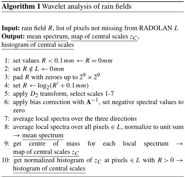
For a first overview of the spatial structure in our data, we apply the complete wavelet analysis (summarized in Algorithm 1) to each of the 127×22 rain fields. The resulting mean spectra and scale histograms are then averaged over days related to different weather situations (Fig. 4). We observe that purely convective cases, where thunderstorms occurred without direct connection to a frontal structure, are clearly recognized as small in scale, with energy peaking at scale five (panel a) and the most frequent central scale being near four. The reverse situation, i.e., fronts without significant thunderstorm activity, is characterized by a shift of energy towards larger scales (energy concentrated at scale seven, most centres near scale six). The forecast ensemble and REA2 agree closely on this regime behaviour; the relatively tight spread encompasses the observed spectra in nearly all cases. The fact that almost no variability resides on scales 1 and 2 is hardly surprising since the effective resolution of the COSMO model, below which all processes are unrealistically damped, is at 4 to 5 grid boxes (Bierdel et al., 2012).

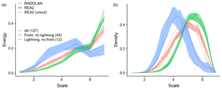
Figure 4 Normalized spatial mean spectra (a) and histograms of central scales (b), averaged over cases with fronts and no convection (green), convection and no fronts (blue), and all cases (red). Areas indicate the range of these mean curves over the 20 ensemble members. Solid and dashed lines correspond to REA2 and RADOLAN, respectively. The dotted line represents the REA2 spectra obtained without masking the fields with the available RADOLAN data.

For the purely frontal cases, as well as the overall climatology, precipitation in RADOLAN lives on systematically smaller scales than in the two model-based data sets, with histograms shifted by about 0.5, reduced energy at scale seven and increased energy below scale 5. Interestingly, this discrepancy is not evident for the purely convective cases where the curves corresponding to RADOLAN are even closer to the centre of the ensemble range than REA2.

To assess the impact of the imperfect, padded boundary conditions on the climatology of these wavelet spectra, we have repeated the analysis for REA2 without setting pixels missing from RADOLAN to zero (neglecting the second step of Algorithm 1). As one might expect due to the possibility for overall larger features, the resulting curves (dotted lines in Fig. 4) are slightly shifted toward large scales. The effect is, however, small compared to both the spread of the ensemble and the difference between ensemble mean, RADOLAN and REA2.

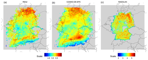
Figure 5 Map of central scales, averaged over all instants with non-zero precipitation for COSMO-REA2 (a), COSMO-DE-EPS (b, averaged over all 20 members) and RADOLAN (c, individual colour bar). Pixels with fewer than 21 d with precipitation were discarded. The RADOLAN mask was not applied to REA2 and COSMO-DE-EPS.

Besides the climatologies of the spatially aggregated wavelet spectra, we are also interested in their average distribution across the domain. The map of central scales allows us to investigate this behaviour in a straightforward manner by simply averaging the locally dominant scales at each pixel over all instances with rain. To ensure that the results are reasonably robust, we only consider grid points with at least three full weeks of non-zero data.

The resulting pattern of average central scales for the reanalysis is shown in Fig. 5a. For this calculation no RADOLAN mask was applied, thus enabling us to study the variability across the complete COSMO-DE domain. We observe that the distribution of predominantly small and large scales is closely tied to the orography: the Alps, Ore Mountains, Black Forest and central German highlands are all associated with decreased central scales. The Baltic Sea, northern German flatlands and Alpine foothills in Bavaria and Austria, on the other hand, tend to experience larger precipitation features.

The corresponding climatological map for the forecasts, averaged here over all ensemble members, is very similar to the reanalysis albeit with slightly larger scales in the southern half of the domain. The picture for RADOLAN, on the other hand, looks completely different (Fig. 5c; note the separate colour scale). Most notably, the overall scales are decreased by roughly 1. Due to the limited area – both the Alps and the Baltic sea are outside the domain – and sharp edges caused by missing data, very little of the structure described above can be recognized.

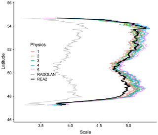
Figure 6 Map of central scales, averaged over all instants with non-zero precipitation and all longitudes. Ensemble members with the same physics setting have the same colour, and RADOLAN and REA2 are black and grey, respectively. Only pixels with available RADOLAN observations and at least 21 d of non-zero rain were included.

For a direct and fair comparison of models and observation, we repeat the calculation of the climatological maps of central scales for REA2 and COSMO-DE-EPS, this time including only pixels for which RADOLAN data are not missing. Noting furthermore that the differences in scale vary mainly in the meridional direction, we average these maps over all longitudes; the results are shown in Fig. 6. In this visualization, we find that the overall pattern of larger scales in southern and northern Germany and smaller scales near the centre is present in all three data sets after all. The RADOLAN profile is qualitatively similar to the others, but shifted down by nearly one scale.

Figure 6 furthermore allows us to assess the differences between groups of ensemble members. Anticipating the results, we have coloured ensemble members according to their physics setting. We find that members with the first physics setting, i.e., an increased entrainment rate (Theis et al., 2014), produce more small-scale variability than the others. Conversely, members with the fifth parameter setting, i.e., increased turbulent length scale, favour large-scale variability. No clear-cut pattern emerges when we sort the ensemble members by their boundary condition (not shown).

Throughout northern and central Germany, the reanalysis lies near the centre of the ensemble spread. In the South, however, all ensemble members produce systematically larger features than REA2. Since the slight discrepancy in internal resolution is constant across the domain, this discrepancy is likely the result of continuous data assimilation.

5 Wavelet-based scores

5.1 Scores based on the mean spectra and scale histograms

Following Buschow et al. (2019), we compare the scale histograms of two rain fields, i.e., forecast and observation, via the earth mover's distance (henceforth EMD): the count in each histogram bin constitutes a pile of earth located at the bin's centre. The EMD is given by the minimum work (dirt moved times distance travelled) required to transport the predicted arrangement of piles into the observed one. We prefer this type of comparison over an element-wise difference because it treats shifts between neighbouring scales appropriately: a displacement from one bin to the next increases the total work and thus the EMD only slightly. A discrepancy by several scales, which would lead to the same element-wise difference between the histograms, is punished more strongly. For further details about the merits of the EMD, the reader is referred to Rubner et al. (2000). The EMD between the two scale histograms (henceforth HEMD) constitutes our first wavelet-based score.

The second score, SEMD is analogously given by the EMD between the two normalized and spatially and directionally averaged spectra. Here, the locations of the dirt piles are given by the scales $j\in \mathit{\{}\mathrm{1},\mathrm{\dots },J\mathit{\}}$, the spectral energy corresponds to the amount of dirt. The normalization of the spectra eliminates differences in total intensity and guarantees that the EMD is a true metric, meaning that only perfectly predicted spectra achieve perfect scores.

As mentioned in Buschow et al. (2019), we can obtain a sign associated with the EMD by calculating the distance between the centres of the two curves, i.e., the difference in expectation value for HEMD and the difference in central scale for SEMD. When desired, the sign of these differences can be attached to SEMD and HEMD in order to assess the directions of the forecast errors (too large or too small).

5.2 Case study: 19 June 2011

To get a first impression of the kinds of errors which determine the outcome of our wavelet-based verification, we consider a case study for which the quality of the ensemble members was deemed below average by both of our scores. On 19 June 2011, a secondary depression near the end of its life cycle made landfall on the German North Sea coast and traversed northern Germany during the afternoon hours. Between 15:00 and 16:00 UTC, RADOLAN observed a large-scale rain band near the cyclone's centre in eastern Germany and a large number of smaller, relatively intense, features across the rest of the domain (Fig. 7a). The forecast considered in the example (member five, Fig. 7c) features a single, substantially rounder, larger and smoother field in the east and only a few scattered objects with very low intensity besides. This discrepancy is clearly reflected by a surplus of large-scale variability in both the mean spectra (panel b) and the scale histograms (panel e). The resulting earth mover's distances amount to approximately one full scale in both cases. Here, we have visualized the corresponding transports as river plots (coloured lines between the histograms). Considering the maps of central scales (panels d and f), we find that the features in the images are classified just as expected with the large rain band living near scale 5 in RADOLAN and scale 6 in the forecast, while the smaller features lie closer to scales 3 and 4.

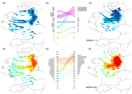
Figure 7 Wavelet-based verification for 19 June 2011 at 16:00 UTC: observed field (RADOLAN, a); observed spectrum, EMD components and forecast spectrum (b); forecast field (Member 5, c). Bottom row: observed map of central scales (d); corresponding histogram, EMD components, forecast scale histogram (e); forecast map of scales (f).

5.3 Case study: 26 February 2011

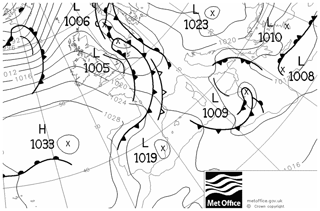
Our second case study similarly features a depression crossing northern Germany. In contrast to the previous example, the dominant weather phenomena are associated not with the cyclone itself, but with its frontal system enclosing a very narrow warm sector which crosses western Germany during the afternoon of 26 February 2011 (Fig. 8). The resulting rain field, as observed by RADOLAN (Fig. 9), consists of two narrow rain bands, one with medium intensity associated with the cold front in the west and one with very low intensities related to the warm front in the east. Neither the reanalysis nor ensemble member 6 exhibit a separation between the precipitation fields of the two fronts, both showing a single broad rain field across south-western Germany instead. Member 1, on the other hand, produces two narrow rain bands, albeit with increased width and length as well as slightly wrong locations compared to RADOLAN.

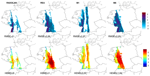
In terms of the overall structure, the first ensemble member is arguably superior to member 6 and REA2. A point-wise verification measure like the root mean square error does not reward the correctly simulated separation into two rain bands. The map of central scales (bottom row of Fig. 9), on the other hand, adequately registers two disjoint rain bands as smaller than the unified pattern. Consequently, member 1 receives a substantially better score (HEMD≈0.5) than member 6 or REA (both close to HEMD=1).

Figure 8 UK Met Office surface pressure chart for 26 February 2011 18:00 UTC (cropped). Contains public sector information licensed under the Open Government Licence v1.0.

Figure 9 Logarithmic rain fields for 26 February 2011 at 19:00 UTC (top row) and corresponding maps of central scales (bottom). From left to right: RADOLAN, REA and COSMO-DE-EPS ensemble members 1 and 6. All fields were cropped to the extent of the available RADOLAN data.

6 Non-wavelet scores

To investigate which properties of a forecast are punished or rewarded by our wavelet-based verification, one natural approach is to compare the scores presented above to alternative verification methods which also focus on the field's structure.

Our first candidate is the structure component of SAL (Wernli et al., 2008, S). For the calculation of S, which is implemented in the SpatialVx R package (Gilleland, 2018), observed and predicted rain field are decomposed into discrete objects. Here, we use the standard algorithm of the R package, which first smooths the data with a simple disc kernel, then discards all pixels below a given threshold R_min and groups continuous regions of non-zero pixels into separate objects. For each object (i), the ratio between total and maximal precipitation is calculated as

$$\begin{array}{}\text{(2)}& V_{\left(i\right)}=R_{\mathrm{tot},\left(i\right)}/R_{max,\left(i\right)},\end{array}$$

where R_tot,(i) and $R_{max,\left(i\right)}$ refer to the total and maximum intensity of the object, respectively. This “peakedness” is averaged over all objects in both fields separately, weighted by R_tot,(i). S is then given by the relative difference in (weighted) mean peakedness of forecast and observation. The sign is chosen such that S>0 indicates forecasts with features that are not peaked enough, i.e., too large and/or too flat.

The key parameter of this procedure is the threshold R_min, which can, depending on the data, have a strong impact on the outcome of the verification (Weniger and Friederichs, 2016). Radanovics et al. (2018) point out that such effects can be minimized as long as thresholds below the respective minimum positive values of the fields are avoided. This property is met by choosing individual thresholds for forecast and observation, truncating each field at 1∕15 of the 95 %-quantile of non-zero values. This approach greatly decreases the computational cost of the procedure since the object decomposition has to be repeated only once per field, not once per combination of observation and forecast. We have checked that the results hardly differ from those obtained with a common threshold.

Our second object of comparison is the weighted p-variogram score of Scheuerer and Hamill (2015). Originally designed for ensemble verification of multivariate quantities, Buschow et al. (2019) adapted this score to a deterministic setting. Assuming stationarity of the data, the score simplifies to the mean squared difference between observed and predicted empirical p variogram, weighted by the inverse distance d⁻¹ between pairs of points, i.e.,

$$\begin{array}{}\text{(3)}& \begin{array}{rl}\mathrm{VGS}& =\sum _{\text{all }\mathrm{0}<d<d_{max}}{d}^{-\mathrm{1}}\left(\sum _{|r_i-r_j|=d}\left|R_{\mathrm{obs}}\right(r_i)\right.\\ & {\left.-R_{\mathrm{obs}}\left(r_j\right){|}^p-\sum _{|r_i-r_j|=d}\left|R_{\mathrm{for}}\right(r_i)-R_{\mathrm{for}}(r_j){|}^p\right)}^{\mathrm{2}}.\end{array}\end{array}$$

Here, R_obs∕for(r_i) denotes the observed or predicted rain value at a given location r_i. In contrast to SEMD, HEMD and S, scores of this form depend explicitly on the variance of the two fields: for p=2, i.e., the classic variogram, the expected squared differences between distant points converges exactly to the variance; changes in this parameter shift the curves up and down. Since we wish to isolate structure from intensity errors, we set p=2 and standardize all fields to unit variance before calculating VGS. This guarantees that all curves converge to the same value; their remaining differences are due to discrepancies in correlation structure. Noting that the inverse distance weighting limits the impact of very distant pairs, we set $d_{max}=\mathrm{50}px$.

In order to check how strongly VGS and the other supposed structure scores depend on intensity errors, we include SAL's amplitude component A, given as the relative difference in total rain, in our experiments as well. All wavelet and non-wavelet scores used in this study are listed in Table 2, the optimal score in each case is zero. The wavelet and variogram transformations are applied to the logarithmic rain fields for the reasons detailed in Sect. 3.2. This transformation is not appropriate for S and A because the resulting negative values lead to unexpected behaviour of the score definitions. These scores are therefore based on the untransformed rain fields for which they were originally developed.

Table 2 All scores used in Sect. 7. J_max and J_min refer to the largest and smallest considered scale of the wavelet decomposition. In this study, $J_{max}-J_{min}=\mathrm{7}-\mathrm{1}=\mathrm{6}$. The optimal value of each score is zero.

7 Verification of COSMO-DE-EPS in 2011

To study the behaviour of our structure verification in aggregate, we apply the wavelet analysis of Algorithm 1 to all 127×22 fields in our data set to obtain the mean spectra and scale histograms on which SEMD and HEMD are based. Similarly, we calculate the total precipitation (basis for A), the average structure function V (Eq. 2, basis for S) and the weighted stationary variogram (basis for VGS). Every field is then compared to every other field, giving us approximately four million realizations of each score listed in Table 2. Different subsets of this large data set are then used to address the following questions:

1. How are these scores related to each other?

2. Can the structure scores discriminate good forecasts from bad ones?

3. How sensitive are the wavelet scores to the choice of mother wavelet, the log-transform, the boundary conditions and the choice of reference data?

The following sections address each of these questions in turn.

7.1 Comparison between scores

For a first overview of the verification results, we consider the distributions of all scores (absolute values) for the 20 forecasts issued on each of the 127 d, verified against RADOLAN. In Fig. 10, we have first separated the resulting distributions by weather situation: days where precipitation was generated by a single type of weather phenomenon (warm front, cold front etc.) are shown in individual box plots, and all other days are grouped into the class “multiple”.

Figure 10 Distribution of absolute values for all scores (matching forecast and observation dates), separated by weather event.

It appears that, at least qualitatively, HEMD, SEMD and VGS are in fair agreement: purely convective days and pure cold fronts (of which our data set contains eight and four cases, respectively; see Fig. 2) were forecast best (lowest scores), followed by warm fronts and other fronts. S agrees in the convective cases, but sees no clear differences between the front types. The two pure convergence-line cases received the unanimously worst scores, but the small sample size prohibits any general conclusions from this observation. The amplitude score A, which does not measure structural properties, shows no great variation across weather situation, the only exception being the four cold-front cases, the total amplitude of which was predicted unusually well.

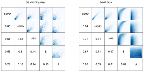
Figure 11 Lower triangle: correlations between the absolute values of all scores, calculated over (a) the 20×127 pairs belonging to matching days and (b) all $\mathrm{20}\times \mathrm{127}\times \mathrm{127}$ combinations of forecast and observation. The upper triangles show bi-variate histograms for all combinations of scores.

To quantify how close the agreement between the different scores actually is, we calculate their correlation matrix, shown in Fig. 11a. Unsurprisingly, the strongest connection is found between the two wavelet scores (0.85), both of which also have a notable connection to the variogram score (0.64 and 0.68). The object-based S is slightly less similar to the other structure scores and shows the closest relationship with the amplitude error A. SEMD, HEMD and VGS, on the other hand, are only weakly linked to A.

To get a broader overview of these interrelations in cases where forecast and observation may be very dissimilar, we have also calculated the same correlations over all possible pairs of forecast and observation date (Fig. 11b). Across this data set, which includes some exceedingly bad predictions, the similarity between all four structure scores increases slightly, and SEMD and HEMD become nearly identical. The connection to the amplitude error A mostly vanishes.

Figure 12 Bi-variate histograms of SEMD and S (a), HEMD and S (b), and SEMD and HEMD (c). The two wavelet scores have been endowed with the sign of the corresponding difference in centre. Percentages indicate the fraction of cases where the two scores have the same sign; cor denotes the correlation.

In the next step, we include the sign of S and endow SEMD and HEMD with the signs of the corresponding centre differences as described in Sect. 5.1. These scores now measure not only the severity of the structural error, but also the direction, i.e., too small or too large. In accordance with the classic SAL definition, the signs are chosen such that positive values indicate a forecast with too much large-scale variability. The joint distributions of the three signed scores are shown in Fig. 12. Here, we have again included all 127×127 combinations of days in order to probe a broad range of good and bad forecasts. HEMD and SEMD agree on the sign of the error in 93 % of cases, and the sign of S matches roughly 85 % of the time. As a result, the correlations rise to cor$(S,\mathrm{HEMD})=\mathrm{0.87}$ and cor$(S,\mathrm{SEMD})=\mathrm{0.85}$, respectively. The bivariate histograms furthermore show that extreme disagreements, which would appear in the upper left and lower right quadrants of the histograms, are rare. The functional relationship of these scores follow a sigmoid-type function.

7.2 Discrimination

The previous section has shown that structure scores based on wavelets, variograms and object properties pass similar, but by no means identical judgement of forecast quality. A natural question is which (if any) of these assessments is correct in the sense that the best forecast receives the best score. In a realistic setting, this question cannot be answered because the objectively best forecast is unknown. As a surrogate, we can consider the ensemble forecast issued for each day as the “correct” prediction and compare it to the 126 forecasts issued for the other days: if the prediction system were perfect and weather patterns never repeated, a sharp verification tool should give the best scores to matching days.

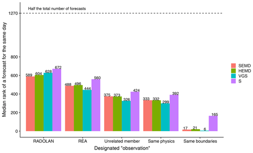
Figure 13 Median rank of the score obtained by the 20 ensemble members belonging to the same day as the observation among the set of all 2540 forecasts. From left to right, the designated “observations” are RADOLAN, REA2, an ensemble member which shares neither boundary conditions nor physics settings with the forecast, an ensemble member which shares the physics settings, and an ensemble member which shares the boundary conditions.

The leftmost bars in Fig. 13 show the median rank of those supposedly best forecasts, verified against RADOLAN. Since there are 20 forecasts per day, the ideal rank is 10. Although such perfect scores are not observed, matching days are nonetheless typically among the 25 % best forecasts, with SEMD issuing the lowest median rank and S the highest. When we use REA2 as the reference instead of RADOLAN, the ranks of all scores improve by about 100 – all structure scores clearly indicate that the COSMO-DE-EPS predictions are structurally more similar to the reanalysis than the observations.

To focus on the discriminatory abilities of our scores, we can take the quality of the predictions out of the equation by selecting a member of the forecast ensemble as the “observation” against which all other forecasts are verified. Ideally, the 20 ensemble members constitute independent realizations from a single distribution which changes from day to day. When forecast and observation share neither physics setting nor boundary conditions (centre of Fig. 13), the rankings for matching days improve with respect to all four scores. In a perfect world, the matching forecasts would rank at number six (since there are 12 unrelated ensemble members). In reality, the ranks are between 326 for VGS and 424 for S. Switching from an unrelated member to an “observation” which shares the forecast's physics settings (of which there are four, making the perfect rank two) only marginally lowers the ranks.

As a final experiment, we select an observation which has the same boundary conditions as the prediction. Visual inspection of example forecast ensembles shows that these members are often extremely similar to one another. As a result, SEMD, HEMD and VGS consider only a handful of other predictions superior to those that share both the boundaries and the date of the observation (rightmost bars in Fig. 13). S, on the other hand, still prefers over 160 other forecasts over the “correct” ones, indicating weaker discriminatory ability.

7.3 Sensitivity of the wavelet scores

Concluding this statistical analysis of our wavelet-based scores, we consider their sensitivity to the free parameters of the method. To this end, the complete verification procedure is repeated three times: once with the Haar wavelet instead of D₂, once without the logarithmic transformation and once without setting pixels missing from RADOLAN to zero. The resulting joint distributions of original and altered scores are shown in Fig. 14. Here, we have again included all pairs of observation and forecast days in the bi-variate histograms (colours).

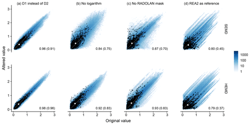
Figure 14 Bivariate histograms of the original wavelet-based scores (on the x axis) against their altered versions (y axis), including all combinations of forecast and observation date. For (a)–(c), RADOLAN is the reference; (d) compares scores against RADOLAN to scores against REA2. Numbers indicate the correlation over all scores, and the number in brackets is the correlation obtained for matching days only (marked by black dots). The white dot represents the mean original and altered values for matching days.

Recalling the outcome of the wavelet selection (Sect. A), as well as the results reported in Buschow et al. (2019), we expect the impact of the chosen mother wavelet to be weak. Figure 14a clearly confirms this expectation: SEMD experiences only minor changes, and the scores remain correlated at 0.96; HEMD is even less sensitive (cor=0.98). We furthermore observe no outliers, indicating that the verdict never changes abruptly as a result of switching from one wavelet to another.

Based on the discussion in Sect. 3.2, we expect the logarithmic transform to have a greater influence on the result of the verification. For SEMD, our expectation is confirmed (cor≤0.85, wide distribution), and HEMD is notably less affected by the change in “colour scale”.

The experiment without the RADOLAN mask (panel c) constitutes an ideal test for the impact of the wavelet-transform's boundary conditions: originally all values beyond the long and complicated edge of the available RADOLAN data were simply set to zero; now we replace them with the actually available model output, i.e., perfect boundary conditions. The resulting difference in scores is comparable in magnitude to that of the logarithmic transform, but the distribution is different. While the overall correlation over all cases is high, the range of occurring differences is broader, meaning that individual fields with prominent features near or beyond the border can experience a strong shift in the verification result. HEMD is again less sensitive than SEMD and produces fewer outliers.

In a final step, we consider the impact of the chosen validation data (Fig. 14d). As one might expect based on the results of previous sections, the change from RADOLAN to REA2 as “observation” can result in completely different verification results, the sensitivity of both scores being similar in this instance.

All correlations discussed so far decrease monotonically when only matching pairs of forecast and observation date, i.e., reasonably good forecasts, are considered (black dots in Fig. 14). The qualitative results remain unchanged; HEMD is the less sensitive score and the mother wavelet has the least impact, while logarithm and boundary condition are more important. The strongest decrease in correlations occurs for the choice of validation data, meaning that, in our data set, the ranking of individual forecasts for matching days changes almost completely depending on the chosen observations. We note, however, that none of the effects discussed in this section has a strong systematic component – the expected scores (white dots in Fig. 14) are nearly unchanged in all four sensitivity experiments.

8 Summary and discussion

This study has applied the wavelet-based pure structure verification of Buschow et al. (2019) to the systematic evaluation of numerical weather predictions against radar observations, as well as a regional reanalysis.

In the first step, we have studied the climatological properties of the local wavelet spectra. Similar analyses of the predicted average spatial structure were carried out by Willeit et al. (2015) and Wong and Skamarock (2016) using Fourier transforms. Aggregation of these mean spectral properties according to the weather situation has confirmed the findings of Brune et al. (2018), who report that wavelet spectra are very well suited to differentiate between rain fields with different degrees of spatial organization. We furthermore find that forecasts and reanalysis, which are based on similar configurations of the same NWP model, have very nearly the same average structure. RADOLAN, on the other hand, is systematically shifted towards smaller scales in most situations. For purely convective rain fields, however, the forecast ensemble is more similar to RADOLAN than to REA2. The latter observation indicates that the discrepancy in scale is not exclusively due to the slight difference in native resolution (1 km for RADOLAN, 2 km for REA2 and 2.8 km for COSMO-DE-EPS) since the grid spacing also differs between forecast and reanalysis and does not depend on the weather situation. By masking the forecasts with the available radar measurements, missing data have been ruled out as a possible explanation as well. We therefore conclude that, irrespective of boundary conditions, physics settings and data-assimilation scheme, the COSMO model tends to produce frontal and other large-scale precipitation patterns which are too large and too smooth.

An evaluation of the temporal mean map of central scales has shown that the discrepancy is mostly constant in space. This step furthermore revealed that the variation in average structure across the ensemble is mostly determined by the physics parametrization. A systematic discrepancy between predictions and reanalysis was furthermore detected over southern Germany. Since the difference in model resolution is constant in space, this observation indicates that the model has an internal tendency to under-represent small-scale variability in this region. Overall this type of climatological analysis has proven to be a useful first evaluation of the average model performance. The natural possibility to localize errors in space constitutes an advantage over the Fourier approach of Willeit et al. (2015) and Wong and Skamarock (2016).

Our second set of results concerns the typical behaviour of the two wavelet-based structure scores SEMD and HEMD. Buschow et al. (2019) report that these scores, as well as the object-based S and the variogram score VGS, can discriminate between good and bad predictions of spatial structure in a controlled environment. Exploiting the fact that each individual forecast ensemble essentially contains 20 draws from an ever-changing probability distribution, we have demonstrated that many of the results previously obtained with synthetic rain fields can be transferred to the real world: all four scores are reasonably good at distinguishing matching forecasts from non-matching ones, S being the worst at this exercise and VGS marginally better than the two wavelet alternatives. Interpreting this experiment, is important to realize that discrimination is not the only desirable property for the scores under consideration, since we also wish to isolate information on the field's structure from all other kinds of errors.

To learn more about the kinds of forecast errors punished by our structure scores, we have considered two selected case studies. Here, HEMD was found to be particularly easy to interpret since we can plot the map of central scales on which it is based. In this manner we found that the score can, for example, reward the correctly predicted split precipitation field in a nearly but not completely occluded frontal system, or punish the lack of small-scale rain features surrounding a secondary depression.

A statistical analysis across the complete data set revealed that, in realistic forecast situations, HEMD and SEMD are usually in very close agreement with each other. The wavelets furthermore typically find the same sign of the error as the object-based S. The moderate correlation between S and the wavelet scores is likely due to low-intensity areas which are removed during the object identification procedure required for SAL, but may have a big impact on the average wavelet spectra. The variogram-based VGS is, on average, more similar to the wavelets. Here, the remaining differences are probably related to the fact that the incarnation of VGS, recommended by Scheuerer and Hamill (2015) and employed in this study, down-weights long-distance correlations while the wavelet spectra treat all scales equitably. It is worth noting that the overall performance of the variogram score is surprisingly good, despite the questionable assumption of spatial stationarity.

Based on the discussion above, we can overall recommend HEMD as a useful tool for purely structural verification of quantitative precipitation forecasts. Its verdict is very similar to that of SEMD, but less sensitive to the choice of the mother wavelet and boundary conditions, and easier to interpret thanks to the underlying map of central scales. We have demonstrated that our score can provide useful additional information on a very specific aspect of forecast performance and should be used in conjunction with other techniques which isolate errors in feature location, intensity and total area.

Another property, which has so far been left out of the analysis, is the orientation and anisotropy of the rain fields. Since several important weather phenomena such as fronts and squall lines have very characteristic anisotropic shapes, these are clearly relevant aspects of forecast quality to which all scores tested in this study are insensitive. We have intentionally removed the directional information from our wavelet spectra because the underlying transformation is invariant under shifts, but not under rotations. Consequently, the perceived degree of anisotropy, as well as the difference in the orientation of two fields, depends on the orientation itself – one could rotate observation and forecast simultaneously in the exact same way and receive a changed verification result. To avoid this problem, future studies will explore the use of different wavelet transforms which have the necessary redundancy in both location and orientation. A second important direction for future research is the application to the problem of wind verification, which faces many of the same issues as precipitation and has recently received much attention in the spatial verification community (Dorninger et al., 2018).

Appendix A: Wavelet selection

In order to objectively select the most appropriate mother wavelet, we follow Goel and Vidakovic (1995), who demonstrate that the similarity between data and basis function can be optimized by minimizing the entropy of the mother wavelet's corresponding orthogonal transform. In a nutshell, wavelets with many vanishing moments and large support areas are good at representing smooth internal structures while shorter wavelets can handle discontinuities better. For a more detailed discussion of this approach and its appropriateness to our application, we refer to Buschow et al. (2019). Applying the same method to synthetic rain fields with tunable smoothness and scale, these authors found that the differences between the Daubechies wavelets are only moderate compared to the difference between parameter settings – the wavelet spectra are determined mostly by the structure of the field, not the shape of the basis function.

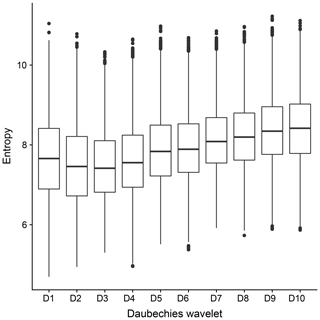
Figure A1 Entropy of the transforms for the first 10 Daubechies wavelets (specifically the “extremal phase” versions). Points denote the median, lines the interquartile range over all forecasts and observations from our data set.

Figure A1, summarizing the entropies for all rain fields from our data set, largely confirms this result. While the optimum lies between one and four vanishing moments, the differences between these wavelets of short to intermediate smoothness are marginal compared to the sample variability across the different fields. Faced with the choice between D₂ and D₃, which have very nearly identical results, we select D₂ because it has a shorter support, thereby allowing us to utilize the first seven scales (see Table 1).