the Creative Commons Attribution 4.0 License.
the Creative Commons Attribution 4.0 License.
 | 30 Apr 2020
Possible impacts of climate change on fog in the Arctic and subpolar North Atlantic
Richard E. Danielson
Minghong Zhang
William A. Perrie
A conventional parameterization of midlatitude warm fog occurrence, based on in situ observations, is employed to estimate marine surface visibility in the Arctic and North Atlantic from three datasets: an ensemble member of the Hadley Earth System (HadGEM2) model and a nested regional WRF simulation that follow historical and future emissions scenarios for 1979–2100, and the ERA-Interim reanalysis for 1979–2004. Over large scales (of an entire year and region), all three gridded datasets agree well in terms of variables like surface air temperature, whose systematic differences seem small by comparison with its predicted change over the course of this century. On the other hand, systematic differences are more apparent in large-scale estimates of relative humidity and visibility. Large differences are attributed to a sensitivity to representation bias that is inherent in the formulation of each individual model and analysis.
Two simple linear calibrations are examined, both of which assume that an in situ based parameterization is broadly consistent with the use of marine (ICOADS) observations of air and dew point temperature as an error-free reference. A single-step calibration is considered that takes the mean and variance of ICOADS frequency distributions as a reference. A two-step calibration is also performed in which ICOADS collocations are taken as a reference for the ERA reanalysis, which in turn is taken as a large-scale reference for the 1979–2004 HadGEM2 and WRF simulations. Both linear calibrations are applied (locally in time and space to air and dew point temperature) to the future climate scenarios of HadGEM2 and WRF. Although ICOADS observations are not error-free and parameterized visibility estimates are unlikely to capture much more than half the variance found in observations, attempts are made to present consistent regional changes in the frequency of high relative humidity, as a proxy for warm fog occurrence. The large-scale decrease in visibility over the 21st century is in the range of 8 %–12 % in the Arctic and 0 %–5 % in the North Atlantic.
- Article
(2124 KB) - Full-text XML
- BibTeX
- EndNote


Available global records reveal regions of increasing fog occurrence over the ocean over long timescales and decreasing occurrence over land. van Oldenborgh et al. (2010) connect a reduction in dense fog to a decrease in European aerosol loading during 1976–2006. Marine visual observations for 1950–2007 reveal a positive summertime trend in at least two parts of the world where fog is most frequent: expansive regions of the western North Pacific and North Atlantic, centered on the Kuril Islands and the Grand Banks, respectively (Dorman et al., 2017). A relative paucity of observations in the Arctic prohibits similar historical analyses, but observed and expected increases in moisture availability and temperature motivate an exploration of both warm and cold fog occurrence (relative to 0 ∘C) in this region as well (Gultepe et al., 2017).
This study seeks to identify baseline long-term changes in warm fog and visibility that might be expected in the Arctic and North Atlantic marine regions. We assert that a growing number of climate simulations (e.g., Collins et al., 2011; Jones et al., 2011; Taylor et al., 2012; IPCC, 2013; Zhang et al., 2019a, b) permit an initial multiyear prediction. Our pragmatic assumption is that the processes resolved by different climate models, explicitly including sub-synoptic and larger scales, provide a basis for estimating the future trend in fog occurrence. Contemporary studies, both observed and modelled (Dorman et al., 2017; Zhang and Lewis, 2017; Tardif, 2017; Koračin, 2017), highlight that fog formation and dissipation are indeed sensitive to these resolved scales. In an attempt to approach the fog-process scales, we apply a regional model downscaling of Hadley Center Earth System model (HadGEM2) global climate simulations (Zhang et al., 2019a, b) to provide an enhanced representation of radiative processes and moist energy transports. As in situ observations provide a complementary measure of such processes, this study can be seen as an extension (by simple statistical modelling) of physical model downscaling.
It is convenient to estimate visibility for various climate scenarios, insomuch as parameterizations are available that employ common climate model variables like surface temperature or relative humidity (e.g., Gultepe and Milbrandt, 2010). With multiple combinations of models and parameterizations, however, there are at least two related challenges to identifying a reasonably consistent baseline change. First, it is well known that different models may seek to represent or support a variable like surface temperature in subtly different ways. Bayesian data assimilation, for example, acknowledges a separate target analysis for each model grid (Lorenc, 1986; Dee, 2005; Janjić et al., 2018). Another familiar inconsistency relates to spatiotemporal representations of a variable by models versus observations (e.g., Mahfouf, 1991; Simmons et al., 2004). Based on a prior averaging of cloud observations, Gultepe et al. (2007) conclude that input data representation is critical for tuned parameterizations of fog and visibility. Of course, differences in representation by separate models, for example, are prevalent even at a common resolution. That is, any aspect of a model may ultimately determine its representation, from initialization and core numerics to physical parameterizations and a final vertical extrapolation to the surface. We may recognize a need to map between two representations, but given sometimes subtle differences in the target of distinct observations, models, and analyses, as well as the challenges of mapping (e.g., Ehret et al., 2012; Maraun, 2016), representation differences are to be expected nonetheless.
A related challenge to identifying a baseline change in relative humidity and visibility is that rudimentary and advanced estimates alike can be sensitive to a representation of the variables used to calculate them. Observational support is given by Gultepe et al. (2019, their Fig. 10), where visibility varies during the course of a day between 50 km and a few meters within a relative humidity range of 92 %–98 %. By convention, fog is defined as visibility of less than 1 km and is often identified with a relative humidity of greater than 95 %. Gultepe and Milbrandt (2010) note that the lack of a consistent representation of surface relative humidity has led to numerous proposed visibility parameterizations, perhaps applicable to one model each. In our search for a baseline change among multiple models, because the calculation of relative humidity and visibility are sensitive to a representation of their input variables, it is instructive to explore whether systematic differences among models can be adjusted to yield so-called homogeneous datasets. In other words, we seek a baseline that nominally employs a common reference of visibility to which all our estimates can be calibrated.
We begin with a parameterization of visibility based on in situ observations of relative humidity with respect to water. Because marine observations (e.g., ships) generally include air and dew point temperature (and thus relative humidity), they provide a proxy representation for the climate models of interest. Following Gultepe et al. (2017), however, a parameterization of warm fog can be more accurately expressed in terms of condensation nuclei, liquid water content, and drop size distribution (among other variables). By comparison, rudimentary parameterizations are sometimes described as yielding a form of “relative humidity mist”. We also acknowledge that a model approximation of warm fog can cover a domain (i.e., a grid box) that is larger than an entire marine fog event. Our chosen parameterization is expected to capture neither the intensity of warm fog events nor processes that govern cold fog below 0 ∘C nor ice fog below about −20 ∘C (Gultepe et al., 2015, 2017). Finally, in selecting an in situ based parameterization, we consider the corresponding in situ representation (i.e., of the input variables air and dew point temperature) to be our target or true representation. Although any estimate of visibility involves a parameterization that is at least partly empirical, and almost as challenging to relate to prognostic model variables as fog itself (Claxton, 2008; Wilkinson et al., 2013; Koračin, 2017), this in situ representation is not necessarily optimal. However, it is a separate ongoing challenge that, even for a precise instrument, measurement error ranging from 10 % to 50 % (and more in Arctic winter conditions) is common (Gultepe et al., 2017).
A somewhat broader accommodation of targets for truth and error is explored in the context of more than one visibility parameterization by Danielson et al. (2019). This parallel exercise points to relative humidity as a key source of information and allows us to focus on an in situ based, midlatitude parameterization. To establish consistent baseline 21st century trends for either the Arctic or North Atlantic, we focus on a homogeneous calibration of gridded historical estimates of surface air and dew point temperature. Such a calibration is called homogeneous because it seeks to make one dataset as consistent as possible with another. In accordance with our assumption of an error-free ICOADS reference, we adopt ordinary linear regression as our statistical calibration model (a justification is given in the Appendix). Ship and fixed platform marine observations are then taken as a large-scale reference for all model simulations, either directly or indirectly via surface variables of the ERA-Interim reanalysis (Simmons et al., 2004, 2010). Individual datasets that nominally overlap with each other during the 1979–2004 historical period are described in Sect. 2. A visibility parameterization and two exploratory methods of linearly reconciling climate model simulations to observations are discussed in Sect. 3. The resulting high relative humidity and low visibility estimates are then used in Sect. 4 to indicate possible 21st century trends in fog. Conclusions are provided in Sect. 5.
2.1 Regional WRF simulations
The HadGEM2 model family is a comprehensive global Earth System model including terrestrial and ocean ecosystems and their carbon cycling, aerosols, and selected chemical constituents (Collins et al., 2011). The model employs 38 levels above the ocean surface and 40 levels below, without the need for flux corrections in daily coupled simulations of its atmospheric (discretized at 1.25∘ latitude by 1.875∘ longitude, i.e., with a resolution of O[100 km]) and oceanic (discretized at 1∘ poleward of 30∘) components. Comments on physical parameterizations of HadGEM2 in relation to downscaled WRF simulations are provided by Zhang et al. (2019a). This study focuses on two regional configurations of the Weather Research and Forecasting (WRF) model, which are driven at lateral and lower boundaries by a selected ensemble member of the HadGEM2 Earth System CMIP5 simulations. Lateral boundaries can be seen in Fig. 1, at least where in situ collocations exist poleward of 60∘ N in the Arctic and 30∘ N in the Atlantic. A computation of dew point temperature and essential mass, motion, and surface boundary conditions for WRF are obtained from the HadGEM2 database of historical (6-hourly for 1979–2004) and representative concentration pathway (RCP) 4.5 and 8.5 emissions scenario (6-hourly for 2005–2100, but with surface variables archived daily) simulations (Taylor et al., 2012; IPCC, 2013).
Two slightly different configurations of the Weather Research and Forecasting (WRF) model are employed for the Arctic and North Atlantic domains. These are subject to 6-hourly boundary forcing and a minor nudging on the interior toward the HadGEM2 upper tropospheric, large-scale flow (Glisan et al., 2013). Both configurations employ the polar-optimized version (3.6) of WRF (Hines et al., 2015) and the same dynamical core (called ARW) with 38 vertical sigma levels, but on 25 km polar stereographic and 30 km Lambert conformal grids, respectively. Parameterizations common to the two domains include those of longwave radiation (Rapid Radiative Transfer Model), land surface (Unified NOAH scheme), planetary boundary layer (Mellor–Yamada–Janjic scheme), and cloud microphysics (Morrison two-moment scheme). The Arctic and North Atlantic simulations differ in terms of their parameterizations of shortwave radiation (respectively, new Goddard scheme versus Rapid Radiative Transfer Model) and cumulus parameterization (Kain–Fritsch versus Grell–Devenyi ensemble scheme). For both the Arctic and North Atlantic simulations, an evaluation of cyclone statistics reveals good agreement with the ERA-Interim reanalysis in comparison to the original HadGEM2 forcing fields (Zhang et al., 2019a, b). During the course of each multidecadal WRF simulation, snapshots of 2 m (surface) variables are obtained every 6 h by extrapolation from the lowest model level (close to 30 m).
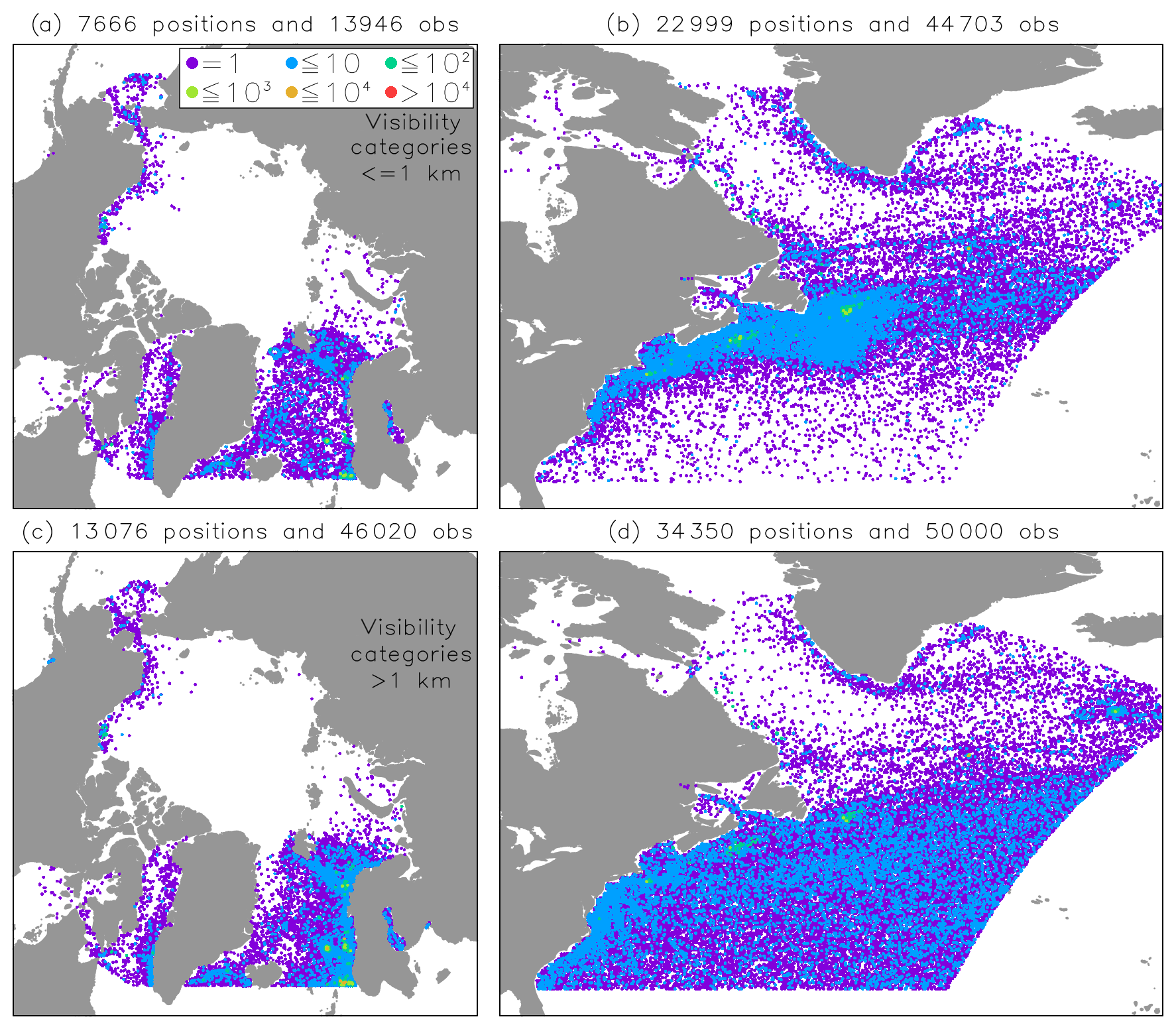
Figure 1Ship and fixed platform marine observations of (a, b) fog and (c, d) non-fog visibility taken between January 1979 and December 2004 to the north of (a, c) 60∘ N in the Arctic and (b, d) 30∘ N in the North Atlantic and within regional WRF model domains. Titles show the total number of ICOADS positions and observations, given at 0.1∘ resolution with order-of-magnitude color labels in (a).
2.2 ERA-Interim reanalysis
A 12-hourly sequential data assimilation system is used in the European Centre for Medium-Range Weather Forecasting Reanalysis (ERA) Interim production of a global atmosphere and ocean surface wave evolution from 1979 onward (Dee et al., 2011). For the atmosphere above the surface, a four-dimensional variational (4D-Var) analysis is performed to obtain model initial conditions and adjustments for selected satellite radiance observations. Within this system, an accommodation of evolving systematic differences between the model and observations is thus made (Dee, 2005). The 4D-Var cost function minimization includes a time-varying specification of error covariance for the prognostic variables and a fixed error covariance for a wide range of observations. A spectral model with 60 vertical levels and an effective horizontal resolution of about 80 km is employed. It is notable that the ERA-Interim 2 m surface variables are not just extrapolated from the lowest model level (like WRF snapshots), but, following Mahfouf (1991), are also combined with in situ observations using an optimal interpolation that is separate from the 4D-Var analysis (Simmons et al., 2004, 2010). Six-hourly surface analyses from 1979 to 2004 are obtained from an archive (Berrisford et al., 2011) that is oversampled at 0.25∘ in latitude and longitude and facilitates land–ocean boundary matching on the WRF Arctic and North Atlantic domains.
2.3 ICOADS observations
In situ surface marine observations of the International Comprehensive Ocean-Atmosphere Data Set (ICOADS Version 3; Freeman et al., 2017) are taken as a reference for diagnoses of visibility between January 1979 and December 2004. To ensure that observations are of high quality, we consider only a full range of valid variables (wind speed and direction, sea level pressure, air, dew point, and sea surface temperature, present weather, and visibility) and the strictest ICOADS trimming (i.e., values of air and sea surface temperature, zonal and meridional wind component, sea-level pressure, and relative humidity are within 2.8 standard deviations of a smoothed monthly climatology). About 1 % of these observations are excluded if any duplication of all variables (including latitude and longitude) is found within a few hours of an existing observation. Also, observations are excluded if any type of precipitation was falling at the time visibility was observed. This is done to emphasize hydrometeors of less than about 30 µm (i.e., fog) in determining visibility (Gultepe et al., 2017).
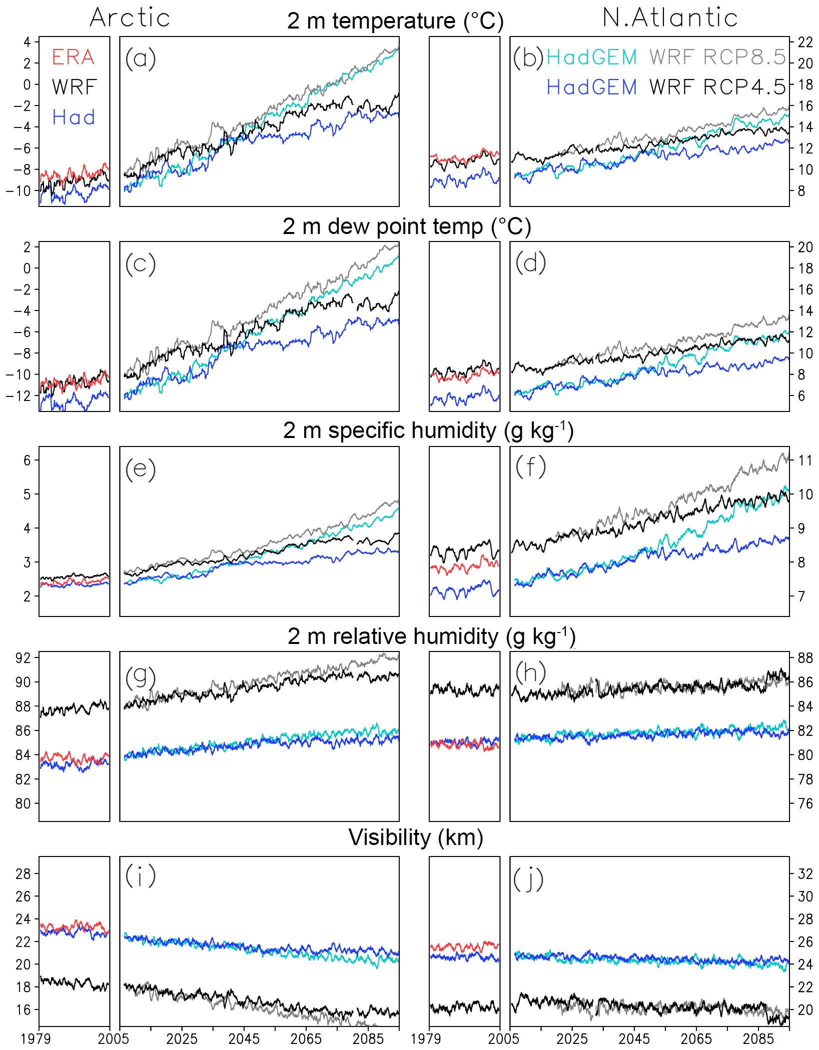
Figure 2Simulated HadGEM2 (blue), WRF (black), and analyzed ERA (red) areal average trends in Arctic (left panels) and North Atlantic (right panels) (a, b) air temperature (∘C), (c, d) dew point temperature (∘C), (e, f) specific humidity (g kg−1), (g, h) relative humidity (%), and (i, j) visibility (km) at 2 m above the surface. The WRF and ERA averages are taken over fixed ocean domains (regardless of sea ice) of 15 (Arctic) and 13 (North Atlantic) million square kilometers. The HadGEM2 domains are about 25 % larger and include coastal overlap as these data are at lower resolution. Note that ordinate scales differ on the left and right, but their spans are equal.
Visibility is recorded in the ICOADS dataset as one of 10 categories ranging from less than 50 m to over 50 km (5 categories of 1 km or less and 5 of 2 km or more). An observer may judge the densest fog categories by the visibility of shipboard objects on large ships, and otherwise by the appearance of the horizon, whose distance is a function of height above the sea (NOAA, 2010). All observations of a given category are selected, but only to a maximum of 10 000 (randomly selected) so as not to emphasize the more common non-fog conditions. Total numbers of fog and non-fog observations, taken from within WRF domains and north of 60∘ N in the Arctic and 30∘ N in the North Atlantic, are shown in Fig. 1. Non-fog observations (Fig. 1c, d) are more distributed geographically and the Arctic fog-only categories (Fig. 1a) are fewer in number. The greatest frequency of observations are at fixed oil platforms and along major shipping routes. High-latitude observations are preferentially from the warm season (Dorman et al., 2017) and data voids occur where sea ice cover is typical. The resulting collocation archive is given by Danielson et al. (2020).
3.1 Visibility parameterization
Uncalibrated estimates of 21st century visibility (Fig. 2) are diagnosed directly from the HadGEM2 and WRF models, following historical emissions (1979–2004) and two future (2005–2100) representative concentration pathway (RCP 4.5 and 8.5) emissions scenarios (Moss et al., 2010; Jones et al., 2011; Taylor et al., 2012; Zhang et al., 2019a, b). Corresponding ERA-Interim visibility estimates are included for the historical period. All variables are averaged over marine regions of the Arctic or North Atlantic model domains using a centered 365 d window. Locally in time and space, surface visibility (Fig. 2i, j) is first diagnosed from relative humidity (Fig. 2g, h), which in turn is derived from temperature (Fig. 2a, b) and dew point (Fig. 2c, d). We estimate visibility using the median curve fit of Gultepe and Milbrandt (2010, ) to be consistent with Danielson et al. (2019), but by their definition of performance, slightly reduced and improved performance is available using the bracketing curve fits that Gultepe and Milbrandt (2010) provide (i.e., their 5 % and 95 % curves, respectively). All curve fits are based on instrument observations of relative humidity and visibility taken during the summers of 2006 and 2007 in Lunenburg, Nova Scotia.
Positive 100-year trends in temperature, dew point, and specific humidity are generally larger than the difference between simulations and the ERA-Interim reanalysis during the historical period, both in the Arctic and North Atlantic. On the other hand, the increase in relative humidity and decrease in visibility (with greater 100-year changes in the Arctic) can be smaller than historical differences among simulations and the ERA analysis. Such a large discrepancy in historical diagnoses of visibility begs the question of how to interpret corresponding future trends. For instance, the HadGEM2 air and dew point temperature estimates are low in part because, in lieu of an interpolation to higher resolution, we opt to average over a larger area that includes some overlap with land. The WRF relative humidity and visibility estimates are different in part because, as snapshots of a long integration, they represent localized supersaturation to a greater extent than other estimates (and in situ observations in particular). Given that our chosen parameterization of visibility itself targets a particular in situ and warm fog representation, which is not necessarily accommodating of such differences, a mapping between each input dataset and an in situ representation is explored.
3.2 Historical linear calibration
The large-scale differences in Fig. 2 seem relatively constant in time, which suggests that representation bias in each gridded dataset is also relatively constant. A reconciliation of gridded data to a highly resolved representation (historical ICOADS observations) is often sought by some combination of physical (e.g., Zhang et al., 2019a, b) and statistical calibration (Ehret et al., 2012; Maraun, 2016), both of which can be considered nonlinear in general. A notable advance in statistical calibration by Freilich and Challenor (1994) established a mapping between two measures of marine wind speed by matching their cumulative distribution functions (CDFs). Mapping between satellite and ERA-Interim soil moisture is examined by Hasenauer (2010), who finds that a linear mapping (by matching the distribution mean and variance) is similar in performance to a nonlinear mapping (including higher moments). Ehret et al. (2012) and Maraun (2016) discuss the benefits and limitations of a range of approaches, such as quantile mapping, which Bennett et al. (2014) employ in a separate calibration of each variable in a multivariate regional climate dataset. More recent studies highlight the importance of simultaneous multivariate calibration (Cannon, 2016, 2018).
Although nonlinear calibration may be appropriate, we explore two linear adjustments because their physical interpretation is direct and the ICOADS reference is assumed to be error-free (comments on calibration to an error-free reference are given in the Appendix). Perhaps the simplest strategy is a two-step calibration, in which we calibrate ERA using the ICOADS collocations in Fig. 1 (step one) and then calibrate HadGEM2 and WRF to ERA (after adjustment) using the values in Fig. 2 (i.e., using large-scale annual and areal averages; step two). Although relative humidity estimates in Fig. 2 could be adjusted to ICOADS directly, instead univariate linear calibrations are applied (locally in space and time) to air and dew point temperature and the remaining variables are calculated from these. We note that an alternate estimate of HadGEM2 visibility is also possible, in which archived daily averages of specific humidity are first calibrated before a dew point estimate is obtained (cf. dew point archival for WRF, ERA, and ICOADS). Unless the HadGEM2 dew point is calculated before it is calibrated, however, differences in Fig. 2 seem to persist (not shown).
Table 1Homogeneous single- and two-step calibrations of Arctic and North Atlantic 2 m air temperature (AT) and dew point temperature (DPT) for 1979–2004. Shown are additive and multiplicative adjustments (left/right numbers) of the ERA reanalysis with reference to all ICOADS collocations in Fig. 1. Similarly, adjustments in WRF and HadGEM2 are with reference to ICOADS in the single-step calibration and with reference to the ERA time series in Fig. 2 (after adjustment) in the two-step calibration. The additive adjustment unit is ∘C.

By construction, the ERA reanalysis has a synoptic correlation with ICOADS observations. The HadGEM2 and nested WRF models follow a distinct synoptic evolution and thus match observations of the 1979–2004 historical period only by coincidence (Taylor et al., 2012; Maraun, 2016). However, a single-step calibration is also feasible that matches the distributions of HadGEM2 and WRF air and dew point temperature to those of ICOADS. Our ordinary linear regression implementation of CDF matching (Freilich and Challenor, 1994; Hasenauer, 2010) adjusts the mean and variance of the gridded in situ collocations over the historical period, after separately ranking both by magnitude. For consistency, ranking is also applied to the ERA and ICOADS collocations, although in a shared synoptic sense, ERA-ICOADS pairings are largely ranked to begin with. In summary, both the single-step and two-step linear calibrations can be considered large-scale adjustments based on the historical collocations of Fig. 1 and the historical areal and annual averages of Fig. 2, respectively.
A linear calibration of collocated air or dew point temperature is capable of matching the mean and variance of HadGEM2, WRF, and ERA distributions to those of ICOADS. In spite of a preexisting conformity of ERA surface variables to in situ observations (Mahfouf, 1991; Simmons et al., 2004, 2010), the assumption of no ICOADS error yields, unsurprisingly, a slight adjustment of ERA temperature and dew point (Table 1). Also as expected, adjustment is smaller (i.e., the additive component is closer to zero and the multiplicative component is closer to one) when the ICOADS and ERA collocation data are separately ranked (single-step) than when they are unranked (two-step, where the first step preserves synoptic pairing). The single-step adjustment of HadGEM2 and WRF generally involves non-negligible additive and multiplicative components, whereas in two-step adjustment (to ERA), the multiplicative component is negligible (equal to one) and the additive component is similar in the Arctic and North Atlantic (cf. Fig. 2). For brevity in the remainder of this section, single-step calibration is discussed in the context of our two-step results.

Figure 3Distribution shifts under a homogeneous two-step calibration. Shown are the fraction of 59 966 Arctic (left panels) and 94 703 North Atlantic (right panels) collocations of Fig. 1, as a function of calibrated (solid lines) and uncalibrated (dashed lines) (a, b) air temperature, (c, d) dew point temperature, and (e, f) relative humidity with respect to water (at 0.5 ∘C and 1 % intervals, respectively, with a three-point smoothing) for the 26-year historical period. Fractions are shown on a logarithmic scale for the ICOADS observations (green lines), ERA reanalysis (red lines), and WRF (black lines) and HadGEM2 (blue lines) models. Note that WRF boundaries are constrained to the HadGEM2 freely evolving synoptic evolution, whereas the ICOADS and ERA collocations sample the observed 1979–2004 synoptic evolution.
Figure 3a–d reveal good similarity in ERA (red) and ICOADS (green) distributions of air and dew point temperature, both before (dashed) and after (solid) calibration. As in Fig. 2, WRF is a nested model whose representation of temperature differs from the HadGEM2 driving model, and both differ somewhat from the ERA and ICOADS distributions. The calibration of HadGEM2 is more apparent than for WRF, with a shift of about 2 ∘C in all temperature distributions (Table 1). Essentially by design, however, differences in the shape of each distribution are unchanged after both the single-step and two-step calibrations. Figure 3e, f reveal greater variation in the representations of relative humidity and less similarity with ICOADS. The contrast with WRF is most apparent, but in general, ICOADS observations sample more evenly a range in relative humidity from 45 % to 50 % to a limit of just over 95 %. In turn, a linear calibration of temperature has the desired impact of shifting all gridded relative humidity distributions towards drier conditions, but because uncalibrated WRF relative humidity is quite frequently high, linear calibration shifts the peak of its distribution by as much as 5 % to 10 %. This occurs following both the single-step and two-step calibrations and highlights the challenge of conserving relationships between variables in univariate (marginal) adjustments (Ehret et al., 2012; Maraun, 2016; Cannon, 2018).
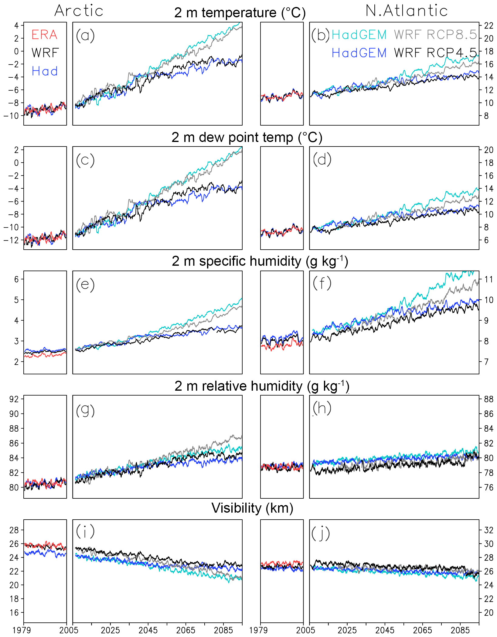
Figure 4As in Fig. 2 but after a homogeneous two-step calibration of the WRF and HadGEM2 simulations to the analyzed ERA time series, which in turn is calibrated to the ICOADS collocations of the historical period (1979–2004).
Comparison of the single-step and two-step calibrations suggests that, in this study, it is more appropriate to employ an additive calibration. As noted above, if ERA-ICOADS differences are ignored, then the single-step calibration is multiplicative, whereas the two-step calibration is additive (Table 1). Both are applied locally in time and space, but unfortunately, the annual and areal averages of a single-step calibration (not shown) do not yield the degree of similarity shown in Fig. 4. Both before (Fig. 2) and after (Fig. 4) two-step calibration, we find that divergence of the RCP4.5 and RCP8.5 trends occurs more so in the Arctic than in the North Atlantic, after 2050, and for temperature, dew point, and specific humidity. The RCP4.5 and RCP8.5 relative humidity and visibility trends are quite similar throughout these simulations. To the extent that relative humidity increases and visibility decreases, this is predominantly found in the Arctic. We estimate the 21st century visibility decrease (in kilometers) to be in the range of 8 %–12 % in the Arctic and 0 %–5 % in the North Atlantic.
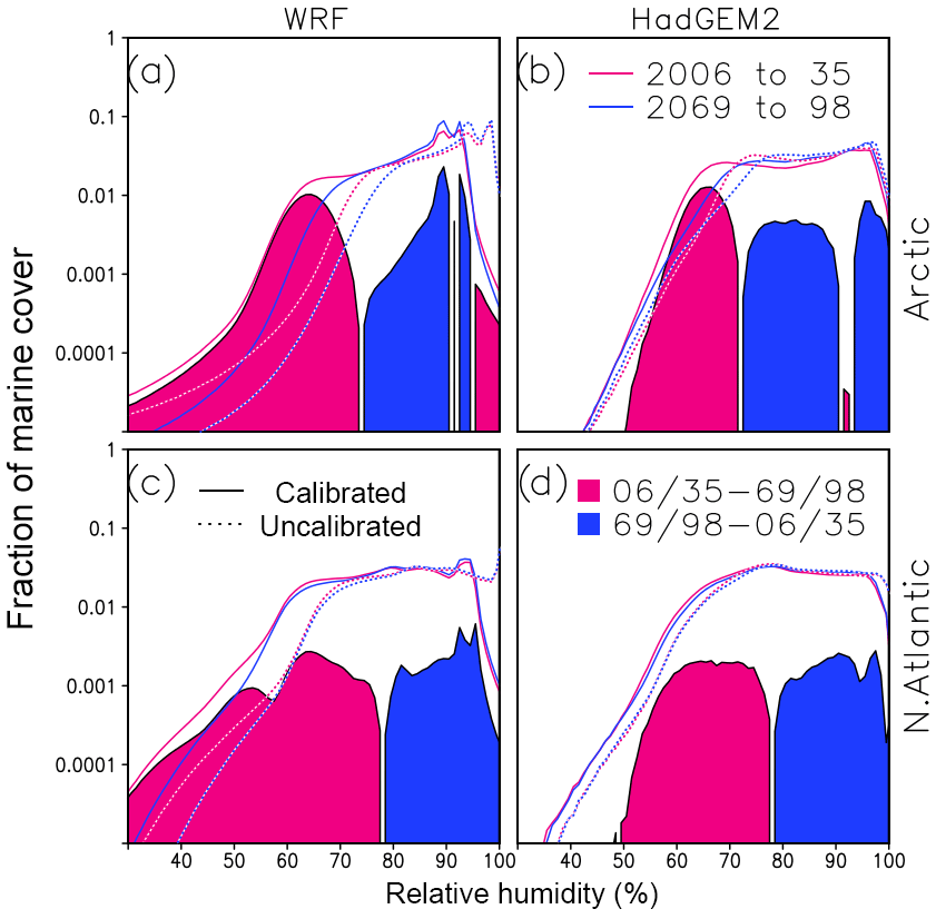
Figure 5Predicted (RCP4.5) distribution shifts in relative humidity with and without a homogeneous two-step calibration. Shown are the fraction of marine coverage as a function of calibrated (solid lines) and uncalibrated (dashed lines) relative humidity with respect to water (at 1 % intervals) for the years 2006–2035 (red lines) and 2069–2098 (blue lines). Fractions are shown on a logarithmic scale for the WRF (a, c) and HadGEM2 (b, d) simulations in the Arctic (a, b) and North Atlantic (c, d). Calibrated positive differences for 2006–2035 minus 2069–2098 (red) and 2069–2098 minus 2006–2035 (blue) are shaded. Note that HadGEM2 relative humidity is obtained from daily averages of air and dew point temperature.
Marine environments of the Arctic and North Atlantic can be characterized by an observed peak in relative humidity that is near saturation, followed by an abrupt limit beyond this value that represents the physical process of condensation, which often includes the fog formation process of interest (Fig. 1a, b). Thus, although our large-scale calibration aligns each distribution with an ICOADS distribution in some mean sense (e.g., with a slight shift in ERA and HadGEM2 relative humidity), accompanying our linear calibration of WRF is the following interpretive burden: there is a notable impact on the frequency of relative humidity near 100 % (i.e., a decrease of about an order of magnitude) and on peak relative humidity (a drying of 5 %–10 %) in the Arctic and North Atlantic. The occurrence of fog is often associated with relative humidity above 95 % (Gultepe and Milbrandt, 2010), and while this is somewhat unchanged in the HadGEM2 calibrated distributions (Fig. 3), its frequency is considerably reduced for WRF.
Figure 5 depicts the impact of linear calibration on the WRF and HadGEM2 RCP4.5 distributions and their 21st century trends in relative humidity (i.e., as a fraction of marine coverage in early and late 30-year periods). The RCP8.5 distributions are nearly the same (not shown). The number of gridded marine samples is 2 to 4 orders of magnitude larger than the number of ICOADS collocations, but as expected, two-step calibration has the same impact as on the historical distributions (Fig. 3). In other words, if we allow that condensational processes are shifted from near 100 % to just greater than 90 % relative humidity in the calibrated WRF RCP distributions, then differences in the early and late 30-year distributions are otherwise the same before and after our simple linear calibration. By accommodating this shift, we find the same signal in Fig. 5 that we find at large scales in Fig. 4. That is, both WRF and HadGEM2 reveal an increase in the frequency of fog-producing (high) relative humidity. The Arctic enhancement in each model (blue shading) is over 10 % of the peak frequency and is roughly double that of the North Atlantic.
The basic premise of this study is that models, observations, and analyses target distinct representations of the marine surface, with similarly distinct forms of bias relative to an unknown, fully supported representation (i.e., the “broad” definition of truth in Ehret et al., 2012). Because we recognize different target representations, there is not necessarily a need to calibrate them.1 We identified a large-scale visibility decrease of about 8 %–12 % in the Arctic and 0 %–5 % in the North Atlantic using HadGEM2 global and WRF nested regional 21st century RCP4.5 climate model simulations. We also identified trends in the frequency of high values of relative humidity, with increases of over 10 % in the Arctic and 5 % in the North Atlantic. Although these represent baseline (calibrated) trends, they are also given directly by the two uncalibrated models. This is desirable because if a calibration is employed, it should not change such trends arbitrarily (Ehret et al., 2012; Maraun, 2016).
The ERA-Interim reanalysis and ICOADS in situ observations provided estimates of marine surface variables complementary to the HadGEM2 global climate model and WRF nested regional model, with its enhanced resolution (Zhang et al., 2019a, b). Temporally constant large-scale differences (Fig. 2) suggested that representation bias in each gridded dataset is also relatively constant.2 We proposed two methods of calibrating linearly (and locally in time and space) air and dew point temperature, from which all other calibrated variables were derived. Estimates of relative humidity and visibility were found to be sensitive to the representation of these two variables. Since our chosen visibility parameterization was formulated based on in situ observations (Gultepe and Milbrandt, 2010), we were motivated to take in situ marine observations as an error-free reference. Although this assumption is unrealistic, it is consistent with our focus on linear calibration (cf. Appendix), and in turn enabled a simple physical interpretation. Of the two methods, a single-step calibration was considered that takes the mean and variance of ICOADS frequency distributions as a reference (Hasenauer, 2010). A two-step calibration was also performed in which ICOADS collocations were taken as a reference for the ERA reanalysis, which in turn was taken as a large-scale reference for the 1979–2004 HadGEM2 and WRF simulations. Although the single-step calibration offered more freedom in distribution matching, the two-step calibration provided a greater degree of consistency in the large-scale trends (Fig. 4).
Our rudimentary parameterization of warm fog is applied on relatively large scales and questions remain concerning trends in cold fog occurrence and warm fog intensity. The Appendix also addresses nonlinear calibration and our assumption of an error-free in situ reference, which we have good reason to explore (Freilich and Challenor, 1994; Bennett et al., 2014; Cannon, 2016), along with the need (or lack thereof) for an ERA calibration. A related caveat of this study that is developed separately (Danielson et al., 2019) is that about half of the variance in observed visibility might be associated with physical processes that are not captured by either climate models or reanalyses. Moreover, there may be a more informed division of collocations by which to refine an ERA calibration or a physical justification for calibrating HadGEM2 or WRF more locally than on the entire Arctic or North Atlantic domains (cf. Ehret et al., 2012; Maraun, 2016). This includes consideration of fog formation in relation to changes in sea ice coverage and possibly distinct trends for the Grand Banks during summer and winter. Another question that remains to be explored, following van Oldenborgh et al. (2010), is possible trends in aerosol loading.
Two measurement models are identified here to highlight that ordinary linear regression, as used in this study, is consistent with linear calibration, whereas an experimental but otherwise quite similar model is consistent with nonlinear calibration (Danielson et al., 2019). We write the familiar ordinary linear regression model as
where C (calibrated ICOADS or ERA) is an error-free reference for U (uncalibrated HadGEM2, WRF, or ERA) and both are either ranked or unranked. Error (ϵU) exists only in the uncalibrated data U and the scalars αU and βU represent a linear adjustment by additive and multiplicative components, respectively. Homogeneous calibration by ordinary linear regression seeks to make U as consistent as possible with C, but insofar as C may have errors, this calibration also uses those errors as a reference. To address this, we include an error (ϵ) that is shared between C and U and an error (ϵC) for C that is unshared with U to write a similar measurement model as
This model differs from the standard errors-in-variables model (Fuller, 2006) in its explicit accommodation of a so-called nonlinear shared error (ϵ). Regardless of whether shared error is written as part of the unshared errors (ϵC and ϵU), however, Eq. (A2) avoids the common assumptions of linear measurements with independent errors (cf. Hall, 2010).
Although calibration may involve confirmation of improved association3 (Oreskes et al., 1994), under a strictly linear calibration that follows from a solution of either Eqs. (A1) or (A2), no change in association is expected (Bentamy et al., 2017). However, we suggest that improved association would be expected under a nonlinear calibration. But if the association between C and U is presumed to be nonlinear, then we propose that improvements be confirmed by a measurement model that accommodates nonlinearity. Of the two models (A1) and (A2), the latter explicitly accommodates a broad interpretive scope for truth and error, nonlinearity in both C and U, as well as a genuine nonlinear association (ϵ) between them (cf. Pearson, 1902). Demonstration of improved association using a simple neural network is given by Danielson et al. (2019). The present study (e.g., Fig. 3 distribution differences) supports the notion that for common measures of relative humidity and visibility (if not for other processes of interest), perhaps only rarely is association expected to be strictly linear.
The ICOADS, ERA-Interim, and HadGEM2 data are available from separate online archives. Collocations employed by this study for the historical period (1979–2004) are also available online (https://doi.org/10.21963/13169, Danielson et al., 2020).
RED proposed the linear calibration approach and provided an initial literature review and interpretation. MZ and WAP contributed to the literature review and MZ supplied the WRF data. RED prepared the Julia code to identify collocations and perform baseline estimates. All the authors contributed to proofreading and fine-tuning the paper.
The authors declare that they have no conflict of interest.
We thank Ismail Gultepe and an anonymous reviewer for insightful comments on earlier drafts and acknowledge those developing the NCAR/NOAA WRF model, the Met Office Hadley Centre Earth System model family, as well as an international effort over many years to assemble and analyze marine observations, as given by the ERA-Interim and ICOADS datasets. Encouragement from Zhenxia Long, Changshuo Chen, George Isaac, and Bjarne Hansen and beneficial contributions from the Julia language (Bezanson et al., 2017) and Wikipedia communities are also appreciated.
This research has been supported by the Ocean Frontier Institute via the Marine Atmospheric Composition and Visibility project (module A grant), from a Belmont Forum project on Fog Variability in a Warming Arctic and its Impact on Maritime Human Activities (AFV grant), from the Aquatic Climate Change Adaptation Services Program of Fisheries and Oceans Canada, and from the Canadian Office of Energy Research and Development (grant no. 1B00.003C).
This paper was edited by William Hsieh and reviewed by Ismail Gultepe and one anonymous referee.
Altman, D. G. and Bland, J. M.: Measurement in medicine: The analysis of method comparison studies, Statistician, 32, 307–317, 1983. a
Bennett, J. C., Grose, M. R., Corney, S. P., White, C. J., Holz, G. K., Katzfey, J. J., Post, D. A., and Bindoff, N. L.: Performance of an empirical bias-correction of a high-resolution climate dataset, Int. J. Climatol., 34, 2189–2204, https://doi.org/10.1002/joc.3830, 2014. a, b
Bentamy, A., Piollé, J.-F., Grouazel, A., Danielson, R. E., Gulev, S. K., Paul, F., Azelmat, H., Mathieu, P.-P., von Schuckmann, K., Sathyendranath, S., Evers-King, H., Esau, I., Johannessen, J. A., Clayson, C. A., Pinker, R. T., Grodsky, S. A., Bourassa, M., Smith, S. R., Haines, K., Valdivieso, M., Merchant, C. J., Chapron, B., Anderson, A., Hollmann, R., and Josey, S. A.: Review and assessment of latent and sensible heat flux accuracy over global oceans, Remote Sens. Environ., 201, 196–218, https://doi.org/10.1016/j.rse.2017.08.016, 2017. a
Berrisford, P., Dee, D., Poli, P., Brugge, R., Fielding, K., Fuentes, M., Kållberg, P., Kobayashi, S., Uppala, S., and Simmons, A.: The ERA-Interim archive Version 2.0, ERA Report Series No. 1, available at: https://www.ecmwf.int/en/elibrary/8174-era-interim-archive-version-20 (last access: October 2018), 2011. a
Beven, K.: Towards a methodology for testing models as hypotheses in the inexact sciences, P. Roy. Soc. A-Math. Phy., 475, 1–19, https://doi.org/10.1098/rspa.2018.0862, 2019. a
Bezanson, J., Edelman, A., Karpinski, S., and Shah, V. B.: Julia: A fresh approach to numerical computing, SIAM Rev., 59, 65–98, https://doi.org/10.1137/141000671, 2017. a
Bland, J. M. and Altman, D. G.: Statistical methods for assessing agreement between two methods of clinical measurement, Lancet, 327, 307–310, https://doi.org/10.1016/S0140-6736(86)90837-8, 1986. a
Cannon, A. J.: Multivariate bias correction of climate model output: Matching marginal distributions and intervariable dependence structure, J. Climate, 29, 7045–7064, https://doi.org/10.1175/JCLI-D-15-0679.1, 2016. a, b
Cannon, A. J.: Multivariate quantile mapping bias correction: An N-dimensional probability density function transform for climate model simulations of multiple variables, Clim. Dynam., 50, 31–49, https://doi.org/10.1007/s00382-017-3580-6, 2018. a, b
Claxton, B. M.: Using a neural network to benchmark a diagnostic parameterization: The Met Office’s visibility scheme, Q. J. Roy. Meteor. Soc., 134, 1527–1537, 2008. a
Collins, W. J., Bellouin, N., Doutriaux-Boucher, M., Gedney, N., Halloran, P., Hinton, T., Hughes, J., Jones, C. D., Joshi, M., Liddicoat, S., Martin, G., O'Connor, F., Rae, J., Senior, C., Sitch, S., Totterdell, I., Wiltshire, A., and Woodward, S.: Development and evaluation of an Earth-System model – HadGEM2, Geosci. Model Dev., 4, 1051–1075, https://doi.org/10.5194/gmd-4-1051-2011, 2011. a, b
Danielson, R. E., Perrie, W. A., and Zhang, M.: A measurement model that offers a partial explanation of variance in marine visibility observations, Fog Project document, 2019. a, b, c, d, e
Danielson, R. E., Zhang, M., and Perrie, W. A.: Collocations of selected in situ (ICOADS) observations and five centred samples of analysis (ERA Interim) and global (HadGEM2) and regional (WRF) numerical model surface marine data, Canadian Cryospheric Information Network online data archive, https://doi.org/10.21963/13169, 2020. a, b
Dee, D. P.: Bias and data assimilation, Q.. J. Roy. Meteor. Soc., 131, 3323–3343, https://doi.org/10.1256/qj.05.137, 2005. a, b
Dee, D. P., Uppala, S. M., Simmons, A. J., Berrisford, P., Poli, P., Kobayashi, S., Andrae, U., Balmaseda, M. A., Balsamo, G., Bauer, P., Bechtold, P., Beljaars, A. C. M., van de Berg, L., Bidlot, J., Bormann, N., Delsol, C., Dragani, R., Fuentes, M., Geer, A. J., Haimberger, L., Healy, S. B., Hersbach, H., Hólm, E. V., Isaksen, L., Kållberg, P., Kohler, M., Matricardi, M., McNally, A. P., Monge-Sanz, B. M., Morcrette, J.-J., Park, B.-K., Peubey, C., de Rosnay, P., Tavolato, C., Thépaut, J.-N., and Vitart, F.: The ERA-Interim reanalysis: configuration and performance of the data assimilation system, Q. J. Roy. Meteor. Soc., 137, 553–597, https://doi.org/10.1002/qj.828, 2011. a
Dorman, C. E., Mejia, J., Koračin, D., and McEvoy, D.: Worldwide marine fog occurrence and climatology, Marine Fog: Challenges and Advancements in Observations, Modeling, and Forecasting, edited: Koračin, D. and Dorman, C. E., Springer, 7–152, https://doi.org/10.1007/978-3-319-45229-6_2, 2017. a, b, c
Ehret, U., Zehe, E., Wulfmeyer, V., Warrach-Sagi, K., and Liebert, J.: HESS Opinions “Should we apply bias correction to global and regional climate model data?”, Hydrol. Earth Syst. Sci., 16, 3391–3404, https://doi.org/10.5194/hess-16-3391-2012, 2012. a, b, c, d, e, f, g
Freeman, E., Woodruff, S. D., Worley, S. J., Lubker, S. J., Kent, E. C., Angel, W. E., Berry, D. I., Brohan, P., Eastman, R., Gates, L., Gloeden, W., Ji, Z., Lawrimore, J., Rayner, N. A., Rosenhagen, G., and Smith, S. R.: ICOADS Release 3.0: A major update to the historical marine climate record, Int. J. Climatol., 37, 2211–2232, https://doi.org/10.1002/joc.4775, 2017. a
Freilich, M. H. and Challenor, P. G.: A new approach for determining fully empirical altimeter wind speed model functions, J. Geophys. Res., 99, 25051–25062, https://doi.org/10.1029/94JC01996, 1994. a, b, c
Fuller, W. A.: Errors in variables, Encyclopedia of Statistical Sciences, edited by: Kotz, S., Read, C. B., Balakrishnan, N., Vidakovic, B. and Johnson, N. L., https://doi.org/10.1002/0471667196.ess1036.pub2, 2006. a
Glisan, J. M., Gutowski Jr., W. J., Cassano, J. J., and Higgins, M. E.: Effects of spectral nudging in WRF on Arctic temperature and precipitation simulations, J. Climate, 26, 3985–3999, https://doi.org/10.1175/JCLI-D-12-00318.1, 2013. a
Gultepe, I. and Milbrandt, J. A.: Probabilistic parameterizations of visibility using observations of rain precipitation rate, relative humidity, and visibility, J. Appl. Meteorol. Clim., 49, 36–46, https://doi.org/10.1175/2009JAMC1927.1, 2010. a, b, c, d, e, f
Gultepe, I., Pagowski, M., and Reid, J.: A satellite-based fog detection scheme using screen air temperature, Weather Forecast., 22, 444–456, https://doi.org/10.1175/WAF1011.1, 2007. a
Gultepe, I., Zhou, B., Milbrandt, J., Bott, A., Li, Y., Heymsfield, A. J., Ferrier, B., Ware, R., Pavolonis, M., Kuhn, T., Gurka, J., Liu, P., and Cermak, J.: A review on ice fog measurements and modeling, Atmos. Res., 151, 2–19, https://doi.org/10.1016/j.atmosres.2014.04.014, 2015. a
Gultepe, I., Milbrandt, J. A., and Zhou, B.: Marine fog: A review on microphysics and visibility prediction, Marine Fog: Challenges and Advancements in Observations, Modeling, and Forecasting, edited by: Koračin, D. and Dorman, C. E., Springer, 345–394, https://doi.org/10.1007/978-3-319-45229-6_7, 2017. a, b, c, d, e
Gultepe, I., Sharman, R., Williams, P. D., Zhou, B., Ellrod, G., Minnis, P., Trier, S., Griffin, S., Yum, S. S., Gharabaghi, B., Feltz, W., Temimi, M., Pu, Z., Storer, L. N., Kneringer, P., Weston, M. J., Chuang, H.-Y., Thobois, L., Dimri, A. P., Dietz, S. J., França, G. B., Almeida, M. V., and Albquerque Neto, F. L.: A review of high impact weather for aviation meteorology, Pure Appl. Geophys., 176, 1869–1921, https://doi.org/10.1007/s00024-019-02168-6, 2019. a
Hall, M. J. W.: Local deterministic model of singlet state correlations based on relaxing measurement independence, Phys. Rev. Lett., 105, https://doi.org/10.1103/PhysRevLett.105.250404, 2010. a
Haraway, D.: Situated knowledges: The science question in feminism and the privilege of partial perspective, Feminist Stud., 14, 575–599, 1988. a
Hasenauer, S.: Bias correction of soil moisture time series from ERS scatterometer and ERA-Interim data for a global 10-year period, EUMETSAT Meteorological Satellite Conference, Córdoba, Spain, available at: https://www.eumetsat.int/website/home/News/ConferencesandEvents/PreviousEvents/DAT_2042511.html (last access: June 2017), 2010. a, b, c
Hines, K. M., Bromwich, D. H., Bai, L., Bitz, C. M., Powers, J. G., and Manning, K. W.: Sea ice enhancements to Polar WRF, Mon. Weather Rev., 143, 2363–2385, https://doi.org/10.1175/MWR-D-14-00344.1, 2015. a
IPCC: Summary for Policymakers, in: Climate Change 2013: The Physical Science Basis. Contribution of Working Group I to the Fifth Assessment Report of the Intergovernmenta Panel on Climate Change, edited by: Stocker, T. F., Qin, D., Plattner, G.-K., Tignor, M., Allen, S. K., Boschung, J., Nauels, A., Xia, Y., Bex, V., and Midgley, P. M., Cambridge University Press, 2013. a, b
Janjić, T., N, N. B., Bocquet, M., Carton, J. A., Cohn, S. E., Dance, S. L., Losa, S. N., Nichols, N. K., Potthast, R., Waller, J. A., and Weston, P.: On the representation error in data assimilation, Q. J. Roy. Meteor. Soc., 144, 1257–1278, https://doi.org/10.1002/qj.3130, 2018. a
Jones, C. D., Hughes, J. K., Bellouin, N., Hardiman, S. C., Jones, G. S., Knight, J., Liddicoat, S., O'Connor, F. M., Andres, R. J., Bell, C., Boo, K.-O., Bozzo, A., Butchart, N., Cadule, P., Corbin, K. D., Doutriaux-Boucher, M., Friedlingstein, P., Gornall, J., Gray, L., Halloran, P. R., Hurtt, G., Ingram, W. J., Lamarque, J.-F., Law, R. M., Meinshausen, M., Osprey, S., Palin, E. J., Parsons Chini, L., Raddatz, T., Sanderson, M. G., Sellar, A. A., Schurer, A., Valdes, P., Wood, N., Woodward, S., Yoshioka, M., and Zerroukat, M.: The HadGEM2-ES implementation of CMIP5 centennial simulations, Geosci. Model Dev., 4, 543–570, https://doi.org/10.5194/gmd-4-543-2011, 2011. a, b
Koračin, D.: Modeling and forecasting marine fog, Marine Fog: Challenges and Advancements in Observations, Modeling, and Forecasting, edited by: Koračin, D. and Dorman, C. E. Springer, 425–475, https://doi.org/10.1007/978-3-319-45229-6_9, 2017. a, b
Lorenc, A. C.: Analysis methods for numerical weather prediction, Q. J. Roy. Meteor. Soc., 122, 1177–1194, 1986. a
Mahfouf, J.-F.: Analysis of soil moisture from near-surface parameters: A feasibility study, J. Appl. Meteorol., 30, 1534–1547, https://doi.org/10.1175/1520-0450(1991)030<1534:AOSMFN>2.0.CO;2, 1991. a, b, c
Maraun, D.: Bias correcting climate change simulations – a critical review, Curr. Clim. Change Rep., 2, 211–220, https://doi.org/10.1007/s40641-016-0050-x, 2016. a, b, c, d, e, f, g
Moss, R. H., Edmonds, J. A., Hibbard, K. A., Manning, M. R., Rose, S. K., van Vuuren, D. P., Carter, T. R., Emori, S., Kainuma, M., Kram, T., Meehl, G. A., Mitchell, J. F. B., Nakicenovic, N., Riahi, K., Smith, S. J., Stouffer, R. J., Thomson, A. M., Weyant, J. P., and Wilbanks, T. J.: The next generation of scenarios for climate change research and assessment, Nature, 463, 747–756, https://doi.org/10.1038/nature08823, 2010. a
NOAA: National Weather Service Observing Handbook No. 1, Marine surface weather observations, available at: http://www.vos.noaa.gov (last access: August 2018), May 2010. a
Oreskes, N., Shrader-Frechette, K., and Belitz, K.: Verification, validation, and confirmation of numerical models in the Earth sciences, Science, 263, 641–646, https://doi.org/10.1126/science.263.5147.641, 1994. a, b, c
Parker, W. S.: Reanalyses and observations: What's the difference?, B. Am. Meteorol. Soc., 97, 1565–1572, https://doi.org/10.1175/BAMS-D-14-00226.1, 2016. a
Pearson, K.: On the mathematical theory of errors of judgement, with special reference to the personal equation, Philos. T. R. Soc., 198, 235–299, 1902. a
Simmons, A. J., Jones, P. D., da Costa Bechtold, V., Beljaars, A. C. M., Kållberg, P. W., Saarinen, S., Uppala, S. M., Viterbo, P., and Wedi, N.: Comparison of trends and low-frequency variability in CRU, ERA-40 and NCEP/NCAR analyses of surface air temperature, J. Geophys. Res., 109, 1–18, https://doi.org/10.1029/2004JD005306, 2004. a, b, c, d
Simmons, A. J., Willett, K. M., Jones, P. D., Thorne, P. W., and Dee, D. P.: Low-frequency variations in surface atmospheric humidity, temperature, and precipitation: Inferences from reanalyses and monthly gridded observational data sets, J. Geophys. Res., 115, 1–21, https://doi.org/10.1029/2009JD012442, 2010. a, b, c
Tardif, R.: Precipitation and fog, Marine Fog: Challenges and Advancements in Observations, Modeling, and Forecasting, edited by: Koračin, D. and Dorman, C. E., Springer, 395–423, https://doi.org/10.1007/978-3-319-45229-6_8, 2017. a
Taylor, K. E., Stouffer, R. J., and Meehl, G. A.: An overview of CMIP5 and the experiment design, B. Am. Meteorol. Soc., 93, 485–498, https://doi.org/10.1175/JTECH-D-12-00008.1, 2012. a, b, c, d
van Oldenborgh, G. J., Yiou, P., and Vautard, R.: On the roles of circulation and aerosols in the decline of mist and dense fog in Europe over the last 30 years, Atmos. Chem. Phys., 10, 4597–4609, https://doi.org/10.5194/acp-10-4597-2010, 2010. a, b
Wilkinson, J. M., Porson, A. N. F., Bornemann, F. J., Weeks, M., Field, P. R., and Lock, A. P.: Improved microphysical parametrization of drizzle and fog for operational forecasting using the Met Office Unified Model, Q. J. Roy. Meteor. Soc., 139, 488–500, https://doi.org/10.1002/qj.1975, 2013. a
Zhang, M., Perrie, W., and Long, Z.: Dynamical downscaling of the Arctic climate with a focus on polar cyclone climatology, Atmos.-Ocean, 57, 41–60, https://doi.org/10.1080/07055900.2017.1369390, 2019a. a, b, c, d, e, f, g
Zhang, M., Perrie, W., and Long, Z.: Sensitivity study of North Atlantic summer cyclone activity in dynamical downscaled simulations, J. Geophys. Res.-Atmos., 124, 7599–7616, https://doi.org/10.1029/2018JD029766, 2019b. a, b, c, d, e, f
Zhang, S. and Lewis, J. M.: Synoptic processes, Marine Fog: Challenges and Advancements in Observations, Modeling, and Forecasting, edited by: Koračin, D. and Dorman, C. E., Springer, 291–343, https://doi.org/10.1007/978-3-319-45229-6_6, 2017. a
Homogeneous linear calibration to a singular in situ reference is prompted by our choice of visibility parameterization, but the symmetry recognized by Haraway (1988), Parker (2016), Beven (2019), and others invites us to consider the reverse calibration of in situ air and dew point temperature using a numerical model or gridded analysis as a reference. Moreover, this accommodation of symmetry may facilitate a less restrictive form of linear calibration.
Linear calibration is useful to address dataset differences that invariably remain, but in a more effective way, some physical differences have already been addressed. Our WRF downscaling of HadGEM2, for instance, reduces differences with the scale of in situ observations. The treatment of other gridded and in situ data (resolution) limits, and their impact on visibility estimation, can also be attempted. Although calibration is not a prescription for how this treatment might be done, it can aid in identifying more direct methods.
Whereas Oreskes et al. (1994) use the word “agreement”, we use the word “association” here, with both concepts appearing as terms in Eqs. (A1) and (A2). Specifically, measurement in medicine often concerns agreement (Altman and Bland, 1983; Bland and Altman, 1986), where calibration coefficients αU and βU are taken as the linear agreement between C and U. Measurement in philosophy often concerns meaningful association (Oreskes et al., 1994), where shared truth t can be taken as the linear association between C and U. While αU, βU, and t are distinct and identifiable, terminology and meaning may vary across fields.