Robust regional clustering and modeling of nonstationary summer temperature extremes across Germany

We use sophisticated machine-learning techniques on a network of summer temperature and precipitation time series taken from stations throughout Germany for the years from 1960 to 2018. In particular, we consider (normalized) maximized mutual information as the measure of similarity and expand on recent clustering methods for climate modeling by applying a weighted kernel-based k-means algorithm. We find robust regional clusters that are both time invariant and shared by networks defined separately by precipitation and temperature time series. Finally, we use the resulting clusters to create a nonstationary model of regional summer temperature extremes throughout Germany and are thereby able to quantify the increase in the probability of observing high extreme summer temperature values (>35 ^∘C) compared with the last 30 years.

1 Introduction

Extremes in temperature have lasting affects on human health (Gasparrini et al., 2017), power consumption (Thornton et al., 2016; Bartos et al., 2016; Burillo, 2019), biodiversity, and ecosystem services (Bellard et al., 2012; Balvanera et al., 2013). As extreme events occur in the tails of probability distributions, studying them allows us to make predictions of rare, and more catastrophic, weather events. For this reason, recent climate literature has become more focused on extreme event statistics (Brown et al., 2008; Cheng et al., 2014; Christidis et al., 2011; Finkel and Katz, 2018).

Modeling extreme events typically involves fitting a generalized extreme value (GEV) probability distribution to these data under the assumption that the parameters of this distribution do not change in time or are “stationary” (Coles, 2001). Climate variability has resulted in challenges to these assumptions. Steady increasing trends in the mean air temperature have been observed worldwide (Hansen et al., 2010; Wergen and Krug, 2010) and have been attributed to anthropogenic green house gas emissions (Erkwurzel et al., 2017; Hansen et al., 2012; Christidis et al., 2011). With the continued warming trend and recurring heat waves sweeping across Europe (Kyselý, 2002; Schär et al., 2004), most recently occurring in the summers of 2015, 2018, and 2019, the need for nonstationary modeling for accurate extreme temperature prediction has become more apparent (Christidis et al., 2015; Hasan et al., 2013; Hamdi et al., 2018; Rahmstorf and Coumou, 2011). We cite Caroni and Panagoulia (2016), Gao and Zheng (2018), and Hamdi et al. (2018) for examples of nonstationary extreme value modeling; however, there are numerous other examples in the literature. Nonstationary adaptations are particularly important for countries that are less equipped to handle these high temperature events, such as Germany (Tomczyk and Sulikowska, 2018; Kosanic et al., 2019).

Along with nonstationary modeling, there is the need to create regional models of extremes as policy making and governmental response are most influenced when extreme weather events are predicted on a larger scale. With the introduction of machine-learning techniques such as maximized modularity algorithms (Newman, 2006; Duch and Arenas, 2005) and spectral clustering (Hastie et al., 2008; Luxburg, 2007) in many scientific areas including genetics, physics, computer science, and neuroscience, among others (Guimera and Amaral, 2005; Treviño et al., 2012; Zscheischler et al., 2012; Azencott et al., 2018), we are better equipped to deal with large data which provide a more accurate, global understanding of networks. These techniques are particularly useful for dense clusters, such as those observed in climate data where meteorological towers are gridded; networks that are affected by many external factors; and where obvious divisions are unknown.

Recently, spectral clustering methods have been shown to provide reasonable clustering results for climate networks defined by a set of time series (Carney et al., 2019); however, these methods may fail when networks with high intra-cluster similarity are considered. We expand on the methods of Carney et al. (2019) by introducing a weighted kernel approach based on a spectral view of the network that allows for more reliable clustering of dense climate networks where simple k-means methods cannot be reliably implemented. This method provides a robust regional clustering of summer temperature time series from meteorological stations throughout Germany. We show that these regions are both time invariant and equivalent over summer temperature and precipitation time series. We use these clusters to create nonstationary regional models of temperature extremes. Our results show a significant increase in the probability of returns for high summer temperature values (>35 ^∘C) for each region in Germany.

This paper is outlined as follows. Section 2 is broken into three parts: Sect.2.1 contains details on the chosen subset of data; Sect. 2.2 provides relevant background on clustering methods and a detailed description of the clustering algorithm; and Sect. 2.3 provides relevant background on extreme value modeling and details on the methods used for regional modeling of summer temperature extremes. Section 3 is broken into two parts: Sect. 3.1 contains results on the clustering algorithm applied to summer temperature and precipitation time series taken from the stations across Germany; and Sect. 3.2 outlines the extreme value results on the station level and their incorporation into the regional models formed from the clustering outcome. Section 4 is a brief summary of the paper containing future work motivated by the results in this paper.

2 Data and methods

2.1 Data

The data in this analysis were taken from the Deutscher Wetterdienst Climate Data Center (DWD CDC, 2018a), which contains climate records from stations across Germany. We use three data sets from the DWD in total: hourly temperature values from 1960 to 2018 (measured in Celsius), hourly precipitation values from 1995 to 2018 (measured in millimeters), and daily precipitation amounts from 1960 to 2018 (measured in millimeters). All three data sets are used in clustering analysis, although only the hourly temperature data set is used for extremes analysis. We choose two precipitation data sets because hourly precipitation values are not available across Germany before 1995 and daily precipitation values do not provide as much resolution. A summary of these data sets can be found in Table 1.

Table 1 DWD data sets used in clustering.

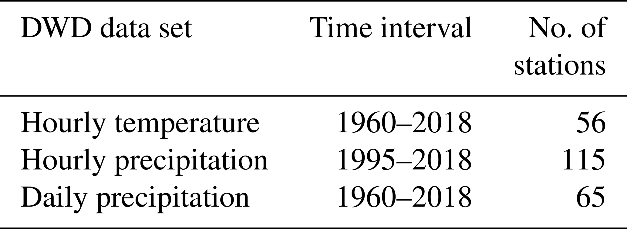
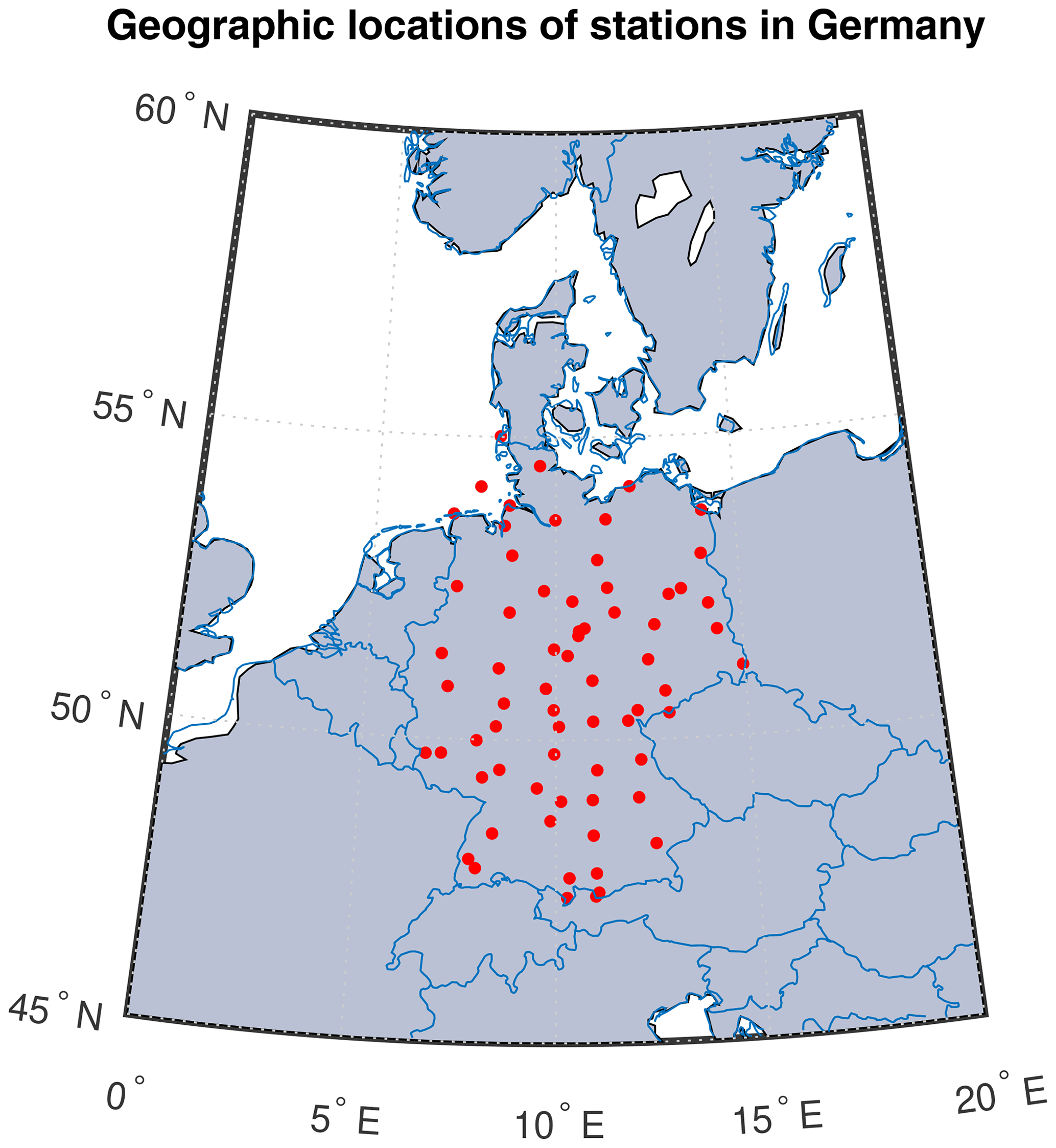
Figure 1 Geographic locations of 68 stations used in regional clustering and modeling of temperature extremes.

The time interval from 1960 to 2018 provides a general representation of all climatology in Germany and a reasonable quantity of extreme values for modeling. For information on station locations used in this analysis, see Fig. 1; detailed station location and identification information can be found in Table A1.

Quality control was performed by the DWD CDC with details provided in Kaspar et al. (2013). We remark that all values used in this analysis passed this preprocessing procedure. These data are not detrended to account for the urban heat island; however, we do not expect this to affect the quality of this analysis because most stations are located several kilometers outside of major cities. With the transfer from manual to automatic weather recording stations, additional considerations are made while investigating the statistical parameters in these data. Some stations in our subset contain missing values; while there are methods that allow us to replace missing data in the time series, such as linear interpolation and the like, these methods require an a priori assumption on the trend in the time series. Stations containing missing values are removed from extremal analysis; however, they are still used for regional clustering because missing data will not notably affect the algorithm.

2.2 Regional clustering

This section discusses some machine-learning tools used to perform regional clustering by viewing the set of time series, corresponding to our subset of weather stations, as a network. The set of time series can be viewed as a weighted network (in graph form: a set of nodes and edges) where each station is a node. The weighted edge between two nodes is calculated by a similarity measure that relies on the corresponding time series (Fig. 2).

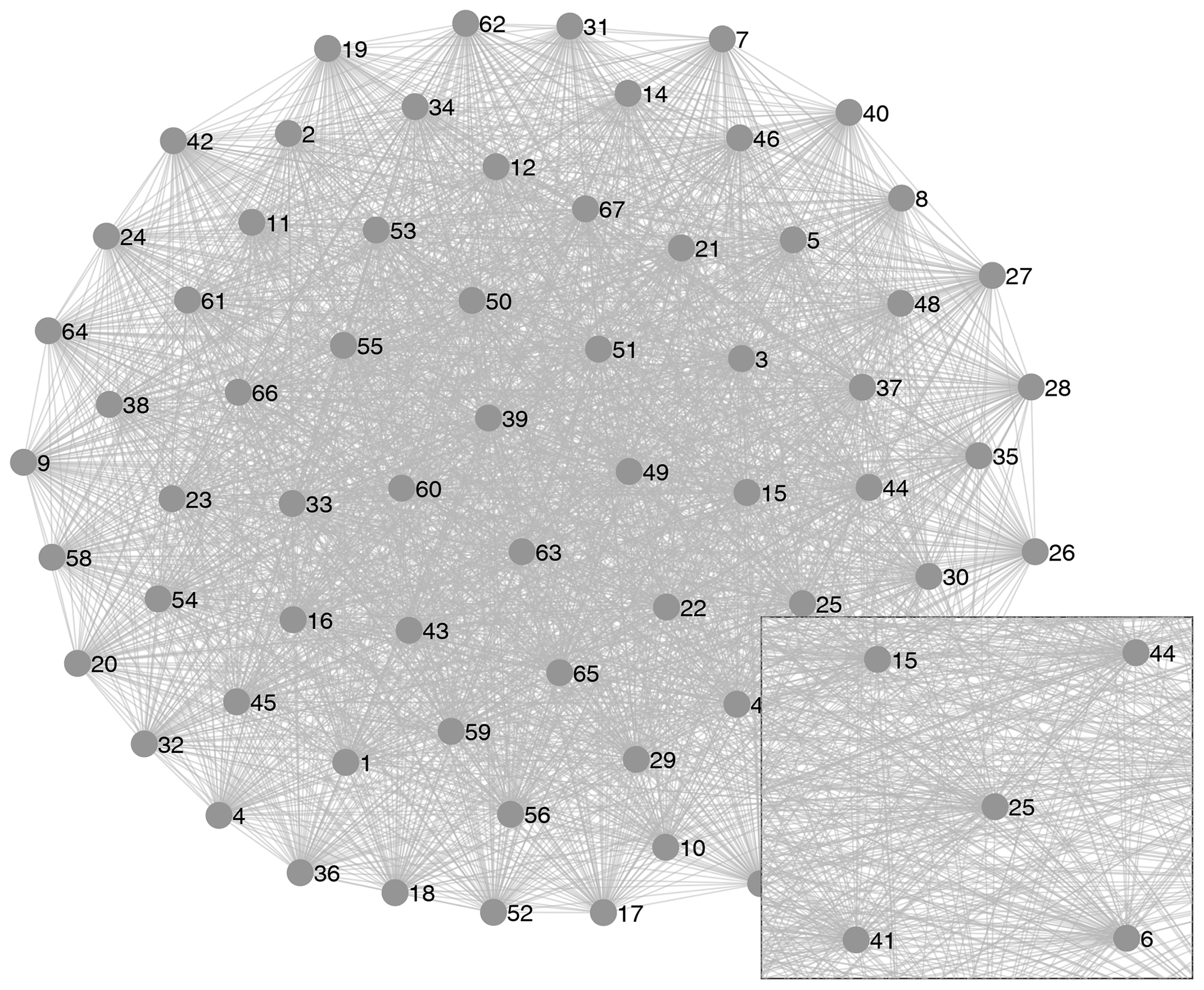
Figure 2 Graphical form of the network defined by temperature time series emphasizing the density of the network. Each node represents a station in the network. Each edge represents a positive similarity between two stations. Note that this graph is not complete because low values of similarity (<0.1) are taken to be zero in this analysis.

Given a network, the goal of clustering analysis is to find a partition with high intra-cluster similarity and low inter-cluster similarity; however, solving this system is an np-hard (non-polynomial) problem. Relaxations of this problem can be split into two approaches: (1) maximizing modularity through partitioning algorithms and redefined modularity metrics (Newman, 2006; Duch and Arenas, 2005; Sun et al., 2009; Li et al., 2008; Chen et al., 2018) or (2) minimizing a distance function through spectral clustering, k-means, and the like (Hastie et al., 2008; Luxburg, 2007; Dhillion et al., 2004). Under standard measures of modularity, Li et al. (2008) showed that these two approaches have an equivalence relation: modularity is maximized if and only if the kernel k-means distance is minimized.

The authors in Carney et al. (2019) approach regional clustering of temperature time series using the spectral clustering method equipped with k-means (Luxburg, 2007). Given n time series, each time series is represented by a point in ℝⁿ where the coordinate is given by the corresponding value of similarity to every time series in the network. The goal of this algorithm is then to find hyperplane separations between the clusters in ℝⁿ by minimizing the objective function defined by the sum of the intra-cluster distances. The spectral portion of this algorithm allows for a reduction in the dimension of the system which results in a set of more easily separable clusters in the lower-dimensional space. The advantage of this approach is that it is computationally efficient and reliable provided that the clusters can be linearly separated. Linear separability is rarely the case with larger, dense clusters (such as in this study) where all similarity measures are close in value. Instead, we employ a weighted Gaussian kernel k-means approach. This method provides a more reliable regional clustering of the time series by allowing the separation of the clusters using a nonlinear function at some computational expense. The weights w_h are given by eigenvalues λ_h of a normalized symmetric, positive definite matrix so that all ${\mathit{\lambda }}_h\in [\mathrm{0},\mathrm{1}]$. These weights serve to compress the clusters along coordinates of less importance, in terms of the corresponding eigenvalue, $w_h={\mathit{\lambda }}_h\ll \mathrm{1}$ and maintain space along coordinates of most importance $w_h={\mathit{\lambda }}_h\approx \mathrm{1}$. We outline the main ideas of the algorithm here; for a more rigorous explanation we refer the reader to the Appendix A1. We also refer to Wang et al. (2019) for a nice introduction on kernel k-means and Hastie et al. (2008, Sect. 14.5.3) and Luxburg (2007) for more information on the spectral portion of this algorithm.

• Step 1. Given any matrix of similarities $S_{i,j}\ge \mathrm{0}$, calculate the normalized Laplacian

  $$\begin{array}{}\text{(1)}& \mathbf{L}={\mathbf{D}}^{-\mathrm{1}/\mathrm{2}}\left(\mathbf{D}-\mathbf{S}\right){\mathbf{D}}^{-\mathrm{1}/\mathrm{2}},\end{array}$$

  where D is the diagonal matrix with entries $D_{i,i}={\sum }_{j=\mathrm{1}}^n{S}_{i,j}$.

• Step 2. Calculate the spectrum of L and choose a cutoff ℓ used to create a subspace of eigenvectors V_h for $h=\mathrm{1},\mathrm{\dots },\mathrm{\ell }$ of L corresponding to the first ℓ eigenvalues.

• Step 3. Calculate the weighted Gaussian kernel

  $$\begin{array}{}\text{(2)}& \begin{array}{rl}& K\left({\widehat{\mathit{W}}}_i,{\widehat{\mathit{W}}}_j\right)=\exp \left(\left[\right|\left|{\widehat{\mathit{W}}}_i\right|{|}^{\mathrm{2}}+{\widehat{\mathit{W}}}_i^T{\widehat{\mathit{W}}}_j\right.\\ & \left.-\left|\right|{\widehat{\mathit{W}}}_j\left|{|}^{\mathrm{2}}\right]/s^{\mathrm{2}}\right),\end{array}\end{array}$$

  where ${\widehat{\mathit{W}}}_i$ and ${\widehat{\mathit{W}}}_j$ are the respective weighted ith and jth row vectors W_i and W_j of the matrix of eigenvectors V_h and s∈ℝ. ${\widehat{\mathit{W}}}_{i,h}=w_h\times W_{i,h}$ where $w_h=\mathrm{1}-{\mathit{\lambda }}_h$.

• Step 4. Run kernel k-means.

  • Step 4.1. Start with k random partitions P_k.

  • Step 4.2. Compute the centers $C_k={\sum }_{m\in P_k}K({\widehat{\mathit{W}}}_m,\cdot )/\text{card}\left(P_k\right)$, where $K({\widehat{\mathit{W}}}_m,\cdot )$ is the mth row vector of the kernel matrix K and card(⋅) is the cardinality function.

  • Step 4.3. Assign ${\widehat{\mathit{W}}}_h$ to the partition P_k with centroid C_k such that

    $$\begin{array}{}\text{(3)}& \sum _k\sum _{{\widehat{\mathit{W}}}_h\in P_k}\left|\right|K({\widehat{\mathit{W}}}_h,\cdot )-C_k|{|}^{\mathrm{2}}\end{array}$$

    is minimized.

  • Step 4.4. Recalculate the centroids based on new assignments of ${\widehat{\mathit{W}}}_h$.

  • Step 4.5. Repeat assignment until a stable minimum is reached.

It is possible that the stable minimum reached is not the global minimum. We run the algorithm for 1000 different initial sets of partitions and choose the cluster associated with the lowest minimized distance. In addition, the number of partitions (clusters) in kernel k-means needs to be assumed a priori. A standard practice is to run the algorithm for different values of k and choose the optimal value as the smallest k corresponding to the greatest decrease in variance. This technique is typically referred to as the “elbow” method Yuan and Yang (2019).

Mutual information has become a more common measurement of similarity in recent literature because it is capable of measuring nonlinear relationships between two time series. For two random variables (or time series) X₁ and X₂ taking discrete values, mutual information is defined as

$$\begin{array}{}\text{(4)}& \mathcal{I}(X_{\mathrm{1}},X_{\mathrm{2}})=\sum _{i=\mathrm{1}}^q\sum _{j=\mathrm{1}}^{q}p(x_{\mathrm{1},i},x_{\mathrm{2},j})\log \left({\displaystyle \frac{p(x_{\mathrm{1},i},x_{\mathrm{2},j})}{p\left(x_{\mathrm{1},i}\right)\cdot p\left(x_{\mathrm{2},j}\right)}}\right),\end{array}$$

where $p\left(x_{\mathrm{1},i}\right)=\mathbb{P}(X_{\mathrm{1}}=x_{\mathrm{1},i})$ and $p(x_{\mathrm{1},i},x_{\mathrm{2},j})=\mathbb{P}(X_{\mathrm{1}}=x_{\mathrm{1},i},X_{\mathrm{2}}=x_{\mathrm{2},j})$. Intuitively, mutual information compares the probability distributions of X₁ and X₂ by measuring their dependence in terms of the joint distribution relative to an assumption of independence. A positive value for Eq. (4) indicates that X₁ and X₂ are dependent in some sense. On the other hand, it is straightforward to see that Eq. (4) equals zero if X₁ and X₂ are independent. We may rewrite mutual information in terms of the entropy of X₁ and X₂ as

$$\begin{array}{}\text{(5)}& \mathcal{I}(X_{\mathrm{1}},X_{\mathrm{2}})=\mathcal{H}\left(X_{\mathrm{1}}\right)+\mathcal{H}\left(X_{\mathrm{2}}\right)-\mathcal{H}(X_{\mathrm{1}},X_{\mathrm{2}}),\end{array}$$

with entropy ℋ(X₁) defined by

$$\begin{array}{}\text{(6)}& \mathcal{H}\left(X_{\mathrm{1}}\right)=-\sum _{i=\mathrm{1}}^{q}p\left(x_{\mathrm{1},i}\right)\log p\left(x_{\mathrm{1},i}\right),\end{array}$$

and joint entropy ℋ(X₁,X₂) given by

$$\begin{array}{}\text{(7)}& \mathcal{H}(X_{\mathrm{1}},X_{\mathrm{2}})=-\sum _{i=\mathrm{1}}^q\sum _{j=\mathrm{1}}^{q}p\left(x_{\mathrm{1},i},x_{\mathrm{2},j}\right)\log p\left(x_{\mathrm{1},i},x_{\mathrm{2},j}\right).\end{array}$$

This reconstruction provides a natural expression of mutual information in terms of information and allows for the calculation of error under the compression of the continuous time series. As the true probability distributions of the data are unknown, a standard approach to calculating the entropy of the time series is to compress the data into discrete bins which form an approximate uniform distribution. From here, the error on the mutual information can be calculated by comparing the resulting compressed distribution with proportion probabilities $\widehat{p}(x_{\mathrm{1},i},x_{\mathrm{1},j})$ to the uniform distribution with equal proportion $p(x_{\mathrm{1},i},x_{\mathrm{1},j})$ (Roulston, 1999).

Compressing the time series can result in an obvious loss of information from the system. Following the work of Carney et al. (2019) and Zhang et al. (2018), we perform gradient ascent by varying the end points of the compression interval to maximize the mutual information between each pair of time series. We will refer to this measurement as the maximized mutual information (MMI). This approach should not change the order of estimated error on the mutual information as entropy is maximized on uniform distributions.

We use a normalized version of the maximized mutual information (NMMI),

$$\begin{array}{}\text{(8)}& \mathcal{U}(X_{\mathrm{1}},X_{\mathrm{2}})=\mathcal{I}(X_{\mathrm{1}},X_{\mathrm{2}})/min\mathit{\left\{}\mathcal{H}\right(X_{\mathrm{1}}),\mathcal{H}(X_{\mathrm{2}}\left)\mathit{\right\}},\end{array}$$

for the network defined by the temperature time series. Normalized versions of the mutual information can produce better clustering results by allowing the mutual information to be viewed relative to the entropy of the time series. In the case of the precipitation network, we find that normalizing the maximized mutual information causes a large error in the spectral decomposition of the normalized Laplacian. This error is a product of naturally low entropy in all time series causing a large value of NMMI and, hence, a large value of D, so that the values of L become too low for optimal spectral decomposition. For this reason, we use the unnormalized version of the maximized mutual information for the precipitation network. Higher values in the entropy for the temperature time series can be attributed to hourly and annual cycles, resulting in a distribution with less dispersion than that of the precipitation time series.

Mutual information may return a large positive value for negatively correlated variables. In this analysis, we cross reference our clustering outcomes from mutual information and correlation. Summer hourly temperature time series (with the daily cycle removed) for all stations in the network are positively correlated. This is expected because Germany is smaller than the average warm air mass. If we attempt to cluster the network by correlation, we find the minimized Euclidean distance plot loses its structure and no longer provides an obvious value for the number of clusters k. We make two observations: first, the correlation network does not allow for reliable clustering of regional temperature values; and, second, mutual information adds substance to the network.

We remark that mutual information provides a reasonable estimate of similarity in the context of clustering extremes because it compares the probability distributions of the time series to determine their shared information. Recent literature has also introduced measures of similarity defined by the extremal index (EI; Bador et al., 2015). This measure incorporates a comparison of the location and scale parameters from the time series’ corresponding GEVs in the sense that two GEVs with equal shape parameters and differing EIs are equivalent up to a shift of their location and scale parameters (Coles, 2001, Theorem 5.2).

2.3 Local and regional extreme value modeling

The block maximum method is used in this analysis to model the maximum values of the time series (Coles, 2001). In this method, the time series is broken into blocks of a chosen length l so that asymptotic results hold: where M is the length of the time series, the number of maximum values is M∕l. Provided the block maxima are independent and stationary, classical extreme value results ensure that they will converge to a generalized extreme value (GEV) distribution described by a shape k, location μ, and scale σ parameter.

$$\begin{array}{}\text{(9)}& F\left(x\right)=\exp [-(\mathrm{1}+k\left({\displaystyle \frac{x-\mathit{\mu }}{\mathit{\sigma }}}\right){)}^{-\mathrm{1}/k}]\end{array}$$

under the requirement $\mathrm{1}+k\left(\frac{x_i-\mathit{\mu }}{\mathit{\sigma }}\right)>\mathrm{0}\forall i$. The shape parameter describes the tail behavior of the maximum values and defines the exact probability distribution to which they will converge, Frechét (Type II) for k>0, Weibull (Type III) for k<0, or Gumbel (Type I) for k=0.

When modeling real-world data, it is natural to use maximum likelihood estimation (MLE; Coles, 2001) or the L-moments method (Hosking and Wallis, 1997) to estimate the three parameters of the GEV model. L-moments is a common technique in climate modeling, and its advantage comes from its stability for low quantities of data (Hosking, 1990); however, the limiting distributions of the estimates are unknown, and bootstrapping methods are required to obtain confidence intervals. Moreover, adaptations to the nonstationary model are not well studied. As we have a relatively large pool of data, maximum likelihood estimation is chosen to estimate the parameters and confidence intervals of the GEV distribution. This is done by maximizing the following log-likelihood function for a set of m block maxima:

$$\begin{array}{}\text{(10)}& \begin{array}{rl}& {\mathcal{L}}_{k,\mathit{\mu },\mathit{\sigma }}=-m\log \mathit{\sigma }-(\mathrm{1}+\mathrm{1}/k)\sum _{i=\mathrm{1}}^m\log \left[\mathrm{1}+k\left({\displaystyle \frac{x_i-\mathit{\mu }}{\mathit{\sigma }}}\right)\right]\\ & -\sum _{i=\mathrm{1}}^m{\left[\mathrm{1}+k\left({\displaystyle \frac{x_i-\mathit{\mu }}{\mathit{\sigma }}}\right)\right]}^{\mathrm{1}/k},\end{array}\end{array}$$

provided that

$$\begin{array}{}\text{(11)}& \mathrm{1}+k\left({\displaystyle \frac{x_i-\mathit{\mu }}{\mathit{\sigma }}}\right)>\mathrm{0}\forall i\end{array}$$

Strict independence is not always necessary for convergence of the maxima to the GEV (Lucarini et al., 2016); however, in practice it is common to choose blocks that are “long enough” for independence to be observed. As temperature time series follow a daily cycle, this daily cycle is removed during independence analysis by subtracting the average cycle over all days in the data. Seasonal cycles are not considered as the data were taken only from summer months. Compression is performed on the centralized data vector by assigning +1 to values that increase in the next step, −1 for values that decrease, and 0 for values that stay the same. These quantities are tabulated, and the chi-square test of independence is performed.

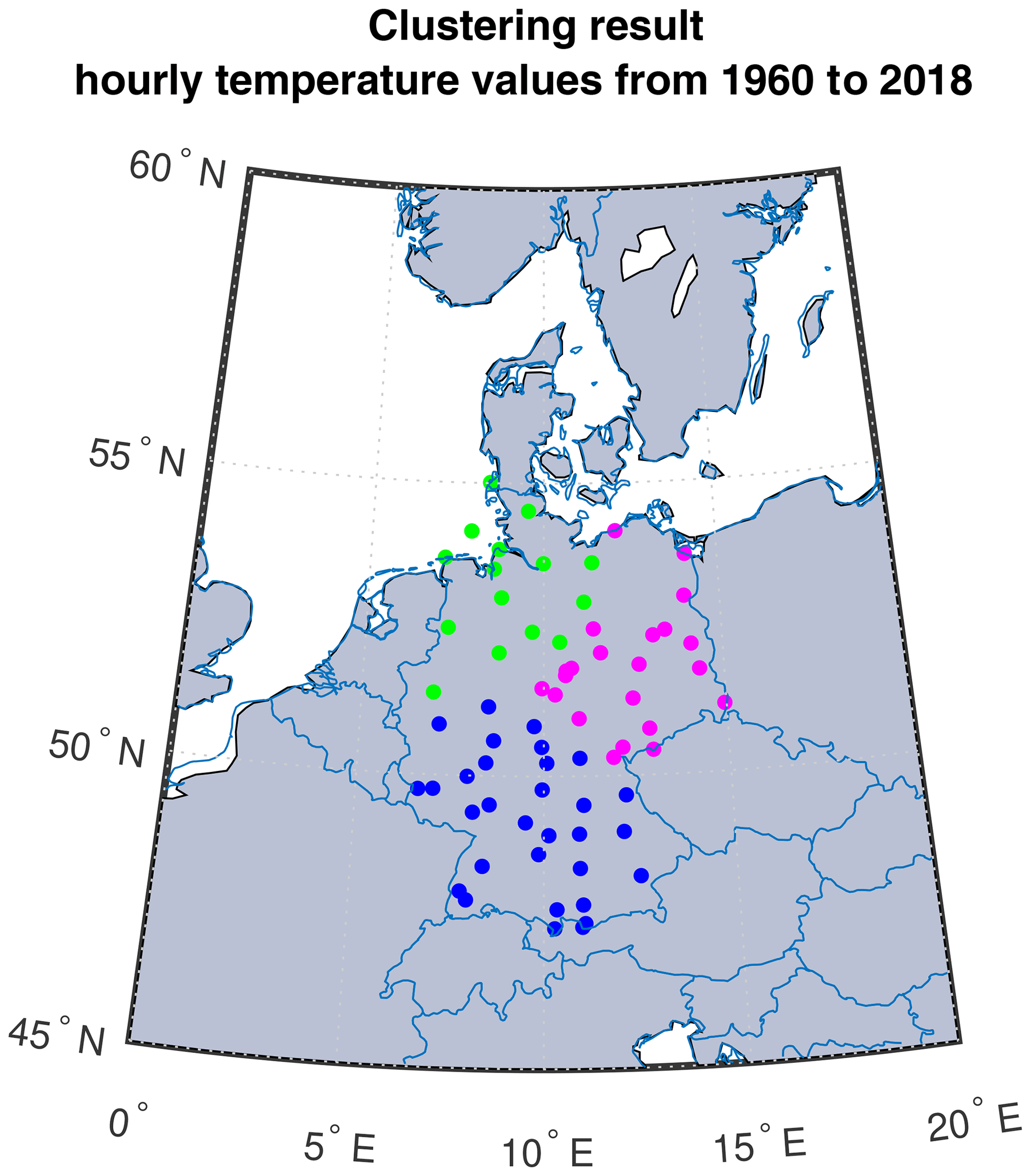
Figure 3 Clustering result for the hourly temperature network with similarity defined by NMMI over the time interval from 1960 to 2018.

Stationary assumptions require the location and scale parameters of the maxima to not change in time. We test this assumption using the Mann–Kendall trend test and a mean difference comparison of the time intervals from 1960 to 1990 and from 1991 to 2018 for the temperature maximum at each station where we find evidence of a linear trended location parameter.

Figure 4 Clustering result for the (a) daily precipitation amounts network taken from the hourly DWD data set with similarity defined by MMI, and (b) the hourly temperature network with similarity defined by NMMI over the time interval from 1995 to 2018.

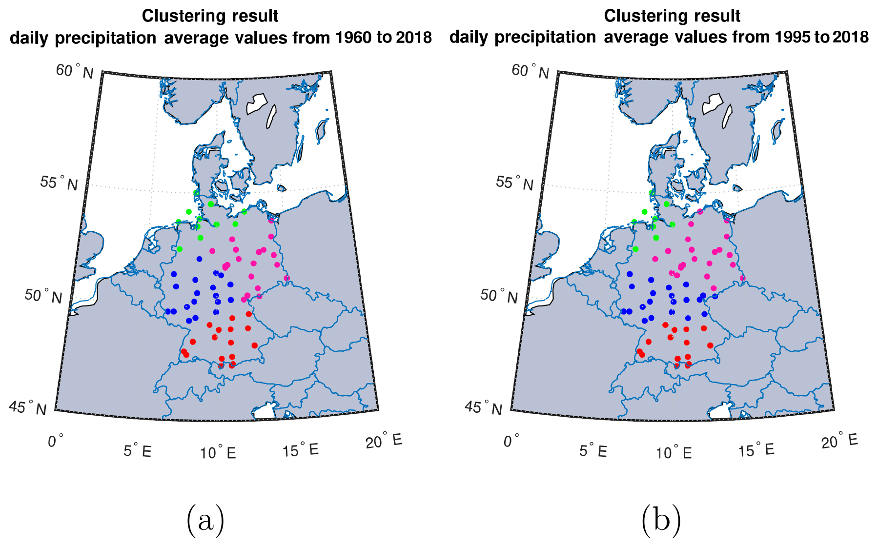
Figure 5 Clustering result for the daily precipitation amounts network taken from the daily DWD data set over (a) the time interval from 1960 to 2018 and (b) the time interval from 1995 to 2018 with similarity defined by MMI.

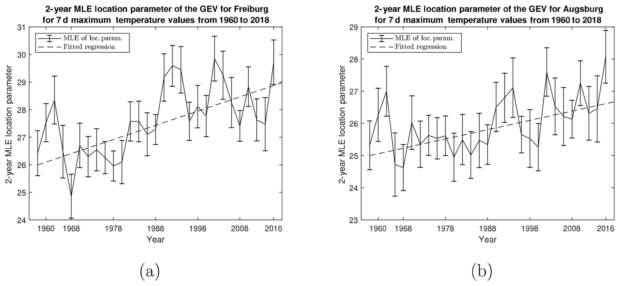
Figure 6 Example time plots for the 2-year maximum likelihood estimate of the location parameter with standard error bars for weekly maximum temperature values taken from (a) Freiburg with fitted regression $y=\mathrm{25.89}+\mathrm{0.10}\times t$ and (b) Augsburg with fitted regression $y=\mathrm{24.94}+\mathrm{0.06}\times t$ (where t is 2-years). Time plots from other stations are similar and can be attributed to the previously mentioned correlations between stations throughout Germany.

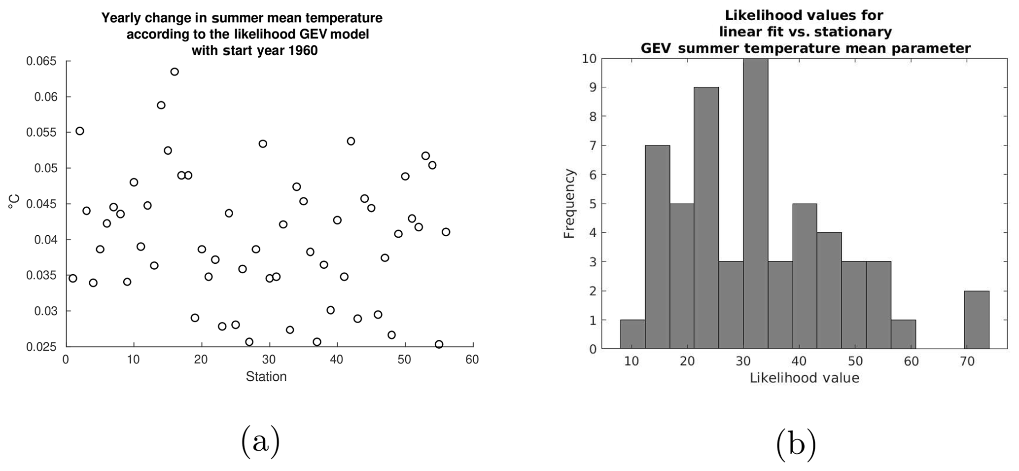
Figure 7 (a) Scatter plot of the yearly change in the temperature mean according to the likelihood GEV model for all stations. (b) Likelihood values comparing the linear fit of the summer temperature mean to that of a stationary mean. All likelihood values surpass the chi-square value of ${\mathit{\chi }}^{\mathrm{2}}(\mathrm{1},\mathrm{0.05})=\mathrm{3.841}$.

Finally, we perform a likelihood-ratio test on the stationary and nonstationary model equipped with a linear time-dependent location parameter $\mathit{\mu }\left(t\right)={\mathit{\beta }}_{\mathrm{0}}+{\mathit{\beta }}_{\mathrm{1}}\times t$. Estimates of the parameters of the nonstationary GEV model were obtained by maximum likelihood estimation of the following log-likelihood function:

$$\begin{array}{}\text{(12)}& \begin{array}{rl}& {\mathcal{L}}_{k,{\mathit{\beta }}_{\mathrm{0}},{\mathit{\beta }}_{\mathrm{1}},\mathit{\sigma }}=-m\log \mathit{\sigma }\\ & -(\mathrm{1}+\mathrm{1}/k)\sum _{i=\mathrm{1}}^m\log \left[\mathrm{1}+k\left({\displaystyle \frac{x_i-\mathit{\mu }\left(t_i\right)}{\mathit{\sigma }}}\right)\right]\\ & -\sum _{i=\mathrm{1}}^m{\left[\mathrm{1}+k\left({\displaystyle \frac{x_i-\mathit{\mu }\left(t_i\right)}{\mathit{\sigma }}}\right)\right]}^{\mathrm{1}/k},\end{array}\end{array}$$

where t_i is the index of a block over which the maxima is taken.

The likelihood-ratio test compares the final log-likelihood values ℒ₁ and ℒ₀ of the nonstationary model ℳ₁ and the stationary model ℳ₀ via the “deviance statistic”:

$$\begin{array}{}\text{(13)}& \mathcal{D}=\mathrm{2}\mathit{\left\{}{\mathcal{L}}_{\mathrm{1}}\right({\mathcal{M}}_{\mathrm{1}})-{\mathcal{L}}_{\mathrm{0}}({\mathcal{M}}_{\mathrm{0}}\left)\mathit{\right\}},\end{array}$$

where 𝒟∼χ²(1). To test whether the resulting nonstationary model fits the data, we transform the original time series of maximum values, Z_t by

$$\begin{array}{}\text{(14)}& {\stackrel{\mathrm{̃}}{Z}}_t={\displaystyle \frac{\mathrm{1}}{k}}\log \left\{\mathrm{1}+k\left({\displaystyle \frac{Z_t-\mathit{\mu }\left(t\right)}{\mathit{\sigma }}}\right)\right\}.\end{array}$$

It is known that ${\stackrel{\mathrm{̃}}{Z}}_t$ follows a stationary Gumbel distribution with μ=0 and σ=1 (Coles, 2001). We perform the Anderson–Darling goodness of fit test on ${\stackrel{\mathrm{̃}}{Z}}_t$ under these assumptions for every station in this analysis.

Regional models are created by formulating a mixed GEV distribution from all of the stations in a regional cluster. The mixed GEV distribution is given by

$$\begin{array}{}\text{(15)}& \begin{array}{rl}& F(z_{\mathrm{1}},\mathrm{\dots },z_N)=\\ & \mathrm{1}/N\sum _{i=\mathrm{1}}^N\exp \left[-{\left(\mathrm{1}+k_i\left({\displaystyle \frac{z_i-{\mathit{\mu }}_i\left(t\right)}{{\mathit{\sigma }}_i}}\right)\right)}^{-\mathrm{1}/k_i}\right],\end{array}\end{array}$$

where N is the number of stations in the regional cluster. This distribution describes the probability of an observed temperature extreme occurring in the regional population defined by the cluster of subpopulations (stations) given an equal probability of sampling from any subpopulation in the regional population. We refer to Yoon et al. (2013) for an example of mixed GEV distributions; however, we remark that fitting results are not required in our context because subpopulations are known.

3 Results and conclusions

3.1 Regional clustering results

As discussed in Sect. 2.2, we compute the maximized mutual information between each pair of stations represented by their corresponding hourly temperature time series from 1960 to 2018. Throughout this analysis, all error for maximized mutual information is on the order of 10⁻⁵. Outcomes of our clustering algorithm applied to the maximized mutual information matrix suggest that Germany has three (k=3) distinct climate regions located in (roughly) the northwest, the northeast, and the south (Fig. 3).

To test for time invariance of the clusters, we apply the algorithm to the intervals from 1960 to 2000, from 1970 to 2010, and from 1980 to 2018. Resulting clusters are equivalent for all three time intervals.

For further investigation, we consider clusters obtained by maximizing the mutual information between pairs of stations represented by their corresponding daily precipitation amounts. Daily precipitation amounts for this analysis are taken from the same hourly recording data set as the temperature data. Precipitation data in this set are only available for the time period from 1995 to 2018. All available data over the period from 1995 to 2018 are used to show the robustness of the regional clusters; however, these data are not used in the final regional cluster analysis of temperature extremes. Hourly precipitation values are summed over each 24 h period and the resulting time series is used to compute the MMI matrix. Clustering results suggest the network of daily precipitation amounts is regionally equivalent to that of hourly temperature (Fig. 4).

For added measure, we consider the daily precipitation amounts taken from the daily DWD CDC set which have values over the same time period (1960–2018) as our temperature data set.

Results from our clustering algorithm show preference for four (k=4) regional clusters over Germany. This fourth cluster is created from a splitting of the southern cluster (Fig. 5). The period from 1995 to 2018 is checked for this data set with similar results. An investigation into the raw data shows slight discrepancies when compared with that of the summed hourly precipitation data which may be the result of differences in the time of recording.

Figure 8 Scatter plot illustrating the difference in mean summer temperature taken over the period from 1960 to 1990 (x axis) and from 1991 to 2018 (y axis) with standard error bars. All values and standard error bars are located above the identity.

3.2 Local and regional extreme value modeling results

For the remaining analysis, we define an extreme (or maximum) value of the temperature time series as the maximum taken over data blocks of 7 d (168 data points). We find independence over almost all blocks at the α=0.05 significance level. The quantity of blocks that do not return independence are less than 5 % and can be attributed to the type I error of the test.

Table 2 Confidence intervals for transformed regional models.

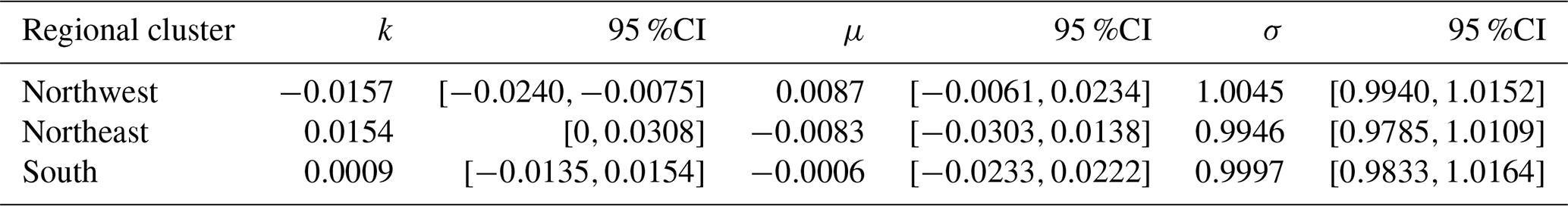
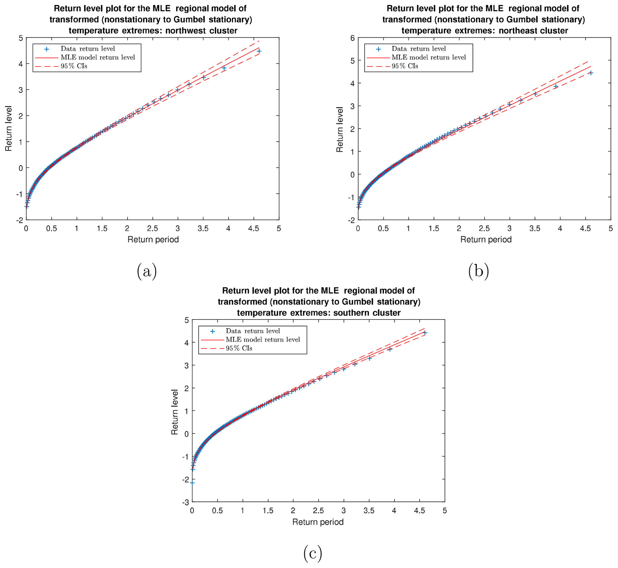
Figure 9 Return level plots comparing the parametric mixed GEV distribution with confidence intervals and actual mixed temperature maxima for the (a) northwest, (b) northeast, and (c) south clusters. These plots emphasize the regional model's fit to the pooled data.

Recall from Sect. 2.3 that fitting a GEV model to the maximum values in a time series requires stationarity of the maximum values, e.g., their location and scale parameters do not change in time. We first test this assumption using the Mann–Kendall trend test on the 2-year (m=24 block maxima) maximum likelihood estimate of the location and scale parameters for weekly summer temperature extremes with the p values indicating that a significant trend (α=0.05) exists for the location parameter and no trend exists for the scale parameter for all stations. We choose 2 years (m=24) of maximum values because this exceeds the minimum sample size requirement for estimating the mean while providing enough data to investigate the trend. Low quantities of block maxima produce larger standard errors on the location parameter. As a way of obtaining additional information to make conclusions regarding the trend, we perform a mean-difference test on the maximum likelihood estimate of the location parameter over the time intervals from 1960 to 1990 and from 1991 to 2018 (m≈373 block maxima per interval) with the alternative hypothesis μ_1991–2018>μ_1960–1990. As the MLE location parameter is asymptotically normal, we use the 95 % confidence intervals to calculate the standard error used in the mean-difference test. We find that this difference is significant (at the α=0.05 significance level) for every station; see Fig. 7 for these results. We also refer the reader to Table A2 for more detailed information. We note that, due to the variability in the location parameter described earlier, low p values from the Mann–Kendall test imply low p values for the mean-difference test, whereas the converse is not true. Time plots are also evaluated as a superficial method of determining whether this trend is the result of a single change-point in the 1990s (Fig. 6). These plots show a continued upward trend, suggesting that this phenomenon is not the result of manual/automatic instrumental change.

Figure 10 Nonstationary generalized extreme value model overlay of 1960 and 2018 weekly temperature extremes for the (a) northwest (b) northeast, and (c) south regional clusters. The shaded region indicates the probability of observing a weekly extreme higher than 35 ^∘C.

Results from these tests provide justification for considering nonstationary modeling of the weekly summer temperature extremes. We use maximum likelihood estimation of the log-likelihood function equipped with a linear trended location parameter to generate the nonstationary GEV model for every station in the data set. We compare these results with the stationary model using the likelihood ratio test, and we find that the nonstationary model provides a significant (α=0.05) improvement over the stationary model for every station; see Fig. 8 for these results. We also refer the reader to Table A3 for more detailed information.

We form regional GEV models using the mixed GEV distribution described by Eq. (14). Stations located at high altitude, including Zugspitze and (the mountains near) Görlitz, were removed from the regional model. These stations have location parameter values that are further than 2 standard deviations away from the regional location parameter. This deviation causes issues with the modality and accuracy of regional temperature extreme probability estimation. When creating regional models of extremes, care needs to be taken regarding the homogeneity of the region in terms of the shape parameter. This is especially important for regional models of extremes where local phenomena are observed. We remark that the mixed GEV distribution has been used to describe regional dynamics with unknown local phenomena through likelihood estimation (Yoon et al., 2013); however, this method is not relevant for our purposes because the subpopulation GEVs (station GEVs) are known and the shape parameters for temperature maxima from each station are nearly equivalent.

To determine how well the regional models represent the pooled time series, we first transform the time series of maxima for each station into a stationary Gumbel distribution using Eq. (13) and perform the Anderson–Darling goodness of fit test on the transformed maxima under the null hypothesis that these data follow a stationary Gumbel distribution with μ=0 and σ=1. We find that all stations follow the null hypothesis at the α=0.05 significance level. Using Eq. (14), we create a transformed (stationary) regional model from the transformed time series that is also expected to follow a Gumbel distribution of μ=0 and σ=1. We perform maximum likelihood estimation on the transformed regional models to test this expectation. All 95 % confidence intervals contain the values μ=0, σ=1, and k=0 (see Table 2). This transformation allows us to create return level plots for the regional model (Fig. 9). Our results suggest that the return levels obtained for the transformed regional model fit the transformed time series. We remark that these return level plots can only be used in model diagnostics to ensure that the regional model is a good representation of the pooled data. Return times for probabilities of temperature maxima exceeding the threshold must be derived from the mixed GEV with a fixed time value.

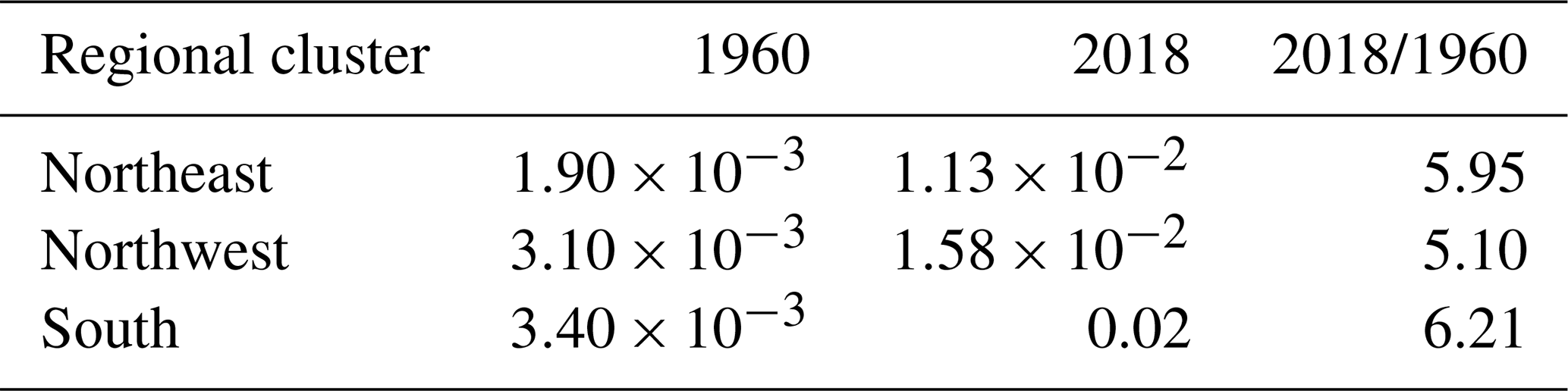
We use the MLE parameters k, μ(t), and σ of the nonstationary GEV models for the mixed GEV regional distribution with fixed t related to the beginning of 1960 and the beginning of 2018. Comparing these models shows an increase in the probability of observing maximum weekly summer temperatures greater than 35 ^∘C of up to 6 times for 2018 compared with 1960 (Fig. 10, Table 3). We remark that the largest difference in the probability of observing an extreme temperature event occurs in the southern cluster, which is likely the result of ocean regulation on the warming trend in the northern clusters (Pörtner et al., 2020).

Table 3 Regional tail probability estimates (in units of occurrences per year) for weekly temperature extremes above 35 ^∘C.

4 Summary

In this analysis, we expand on the work of Carney et al. (2019) by considering a more dense set of networks and adding a weighted kernel k-means approach to the algorithm. This addition allows for more reliable clustering where the k-means method was shown to fail. We find regional clusters for weather stations throughout Germany by defining a network based on their corresponding summer, hourly temperature values. The resulting clusters are not only time invariant but are shared by the network defined by the corresponding daily precipitation amounts. The addition of more stations to the network does not radically change the clustering outcome. Shared clusters could reflect an underlying relationship between temperature and precipitation dynamics. This result is nontrivial because similarity at the station level does not generalize in an obvious way due to the numerous external factors that affect regional weather. We remark that the clustering equivalence does not (necessarily) indicate that temperature and precipitation move together, rather that their individual networks contain relationships between stations within equivalent spacial regions.

We use the clusters we obtain from our algorithm to create regional models of the weekly summer temperature extremes. We find significant increasing linear trends in the location parameter of these models and a preference for nonstationary modeling for all stations in the network. Regional nonstationary models are created by defining a mixed nonstationary GEV distribution from likelihood results. Return time plots are used to validate the results. Regional distribution models reveal an increase in the probability of observing a weekly summer temperature maximum above 35 ^∘C of up to 6 times for 2018 compared with 1960.

In future work, we will consider more complicated networks defined by both temperature and precipitation values, simultaneously. We plan to use these results to form joint probability densities of temperature and precipitation extremes. Viewing the data in this way will allow us to make conclusions about the conditional extreme probabilities. We are also interested in determining whether these clusters are seasonally dependent or consistent throughout the year.

Appendix A: Complementary material

A1 A spectral weighted kernel k-means algorithm

The similarity matrix S_i,j in this study is transformed into the normalized Laplacian given by

$$\begin{array}{}\text{(A1)}& \mathbf{L}={\mathbf{D}}^{-\mathrm{1}/\mathrm{2}}(\mathbf{D}-\mathbf{S}){\mathbf{D}}^{-\mathrm{1}/\mathrm{2}}.\end{array}$$

Spectral decomposition is performed on L, and a matrix is formed with columns given by the first h eigenvectors $[{\mathit{V}}_{\mathrm{1}},\mathrm{\cdots },{\mathit{V}}_h]$ of L. As the Laplacian is normalized, the first h eigenvalues represent the eigenvectors carrying the most information from the network (represented by the Laplacian matrix). The corresponding subspace made of the span of $[{\mathit{V}}_{\mathrm{1}},\mathrm{\cdots },{\mathit{V}}_h]$ is the reduced dimensional network that approximates the true network well. The rows of this matrix correspond to the h-dimensional projections of the input vectors (e.g., the h-dimensional projections of the rows of the similarity matrix). Each row gives a point representation x∈ℝ^h to the stations in the network. The goal of the next step in the algorithm is to find divisions that create clusters of these points in ℝ^h.

Kernel k-means allows for separation of clusters by a nonlinear function. This is done by taking a nonlinear mapping $\mathit{\varphi }\left(x\right):{\mathbb{R}}^h\to \mathcal{F}$ of each input vector x∈ℝ^h into a higher-dimensional (possibly infinite) feature space. Once in the feature space, the goal of clustering is to find partitions that minimize the objective function now given by

$$\begin{array}{}\text{(A2)}& min{\displaystyle \frac{\mathrm{1}}{N}}\sum _{k=\mathrm{1}}^{\mathrm{\ell }}\sum _{j\in P_k}\left|\right|\mathit{\varphi }\left(x_j\right)-{\displaystyle \frac{\mathrm{1}}{\text{card}\left(P_k\right)}}\sum _{i\in P_k}\mathit{\varphi }\left(x_i\right)|{|}_{\mathcal{F}}^{\mathrm{2}},\end{array}$$

where P_k is the kth partition, and i∈P_k indicates the index assigned to P_k. Schölkopf et al. (1998) defined the “kernel trick” by recognizing that ϕ can be viewed as a function on the Hilbert space ℱ equipped with the inner product norm $\langle \cdot ,\cdot \rangle$. This allows us to redefine the objective function

$$\begin{array}{}\text{(A3)}& min{\displaystyle \frac{\mathrm{1}}{N}}\sum _{k=\mathrm{1}}^{\mathrm{\ell }}\sum _{j\in P_k}\left|\right|K(x_j,\cdot )-{\displaystyle \frac{\mathrm{1}}{\text{card}\left(P_k\right)}}\sum _{i\in P_k}K(x_i,\cdot )|{|}_{\mathrm{2}}^{\mathrm{2}}\end{array}$$

in terms of a kernel $K(x_i,x_j)=\langle \mathit{\varphi }\left(x_i\right),\mathit{\varphi }\left(x_j\right)\rangle$. Now, we may minimize the objective function without having to explicitly compute the feature vectors ϕ(x). Choosing K(x_i,x_j) as the Gaussian kernel used in this analysis, given by

$$\begin{array}{}\text{(A4)}& K(x_i,x_j)=\exp \left(-\left|\right|x_i-x_j|{|}^{\mathrm{2}}/s^{\mathrm{2}}\right),\end{array}$$

ensures some universality in the sense that any function required to separate the cluster can be approximated arbitrarily well by a function of the kernel form. The weighted Gaussian kernel is calculated by

$$\begin{array}{}\text{(A5)}& K({\widehat{x}}_i,{\widehat{x}}_j)=\exp \left(\left[\right|\left|{\widehat{x}}_i\right|{|}^{\mathrm{2}}+{\widehat{x}}_i^T{\widehat{x}}_j-\left|\right|{\widehat{x}}_j\left|{|}^{\mathrm{2}}\right]/s^{\mathrm{2}}\right),\end{array}$$

where $w=\mathbf{1}-\overline{\mathit{\lambda }}$; here, $\overline{\mathit{\lambda }}$ is the vector of h first eigenvalues of L and ${\widehat{x}}_{i,h}=w_h\times x_{i,h}$. The values of w represent the amount of information (given by the associated eigenvalue of L) carried by a component of x∈ℝ^h. By using w to weight the input vectors of the kernel, we are able to tighten clusters along coordinates with the least amount of information, or $w_h={\mathit{\lambda }}_h\ll \mathrm{1}$, while maintaining distance along coordinates with the most amount of information, or $w_h={\mathit{\lambda }}_h\approx \mathrm{1}$.

Table A1 DWD station IDs and locations.

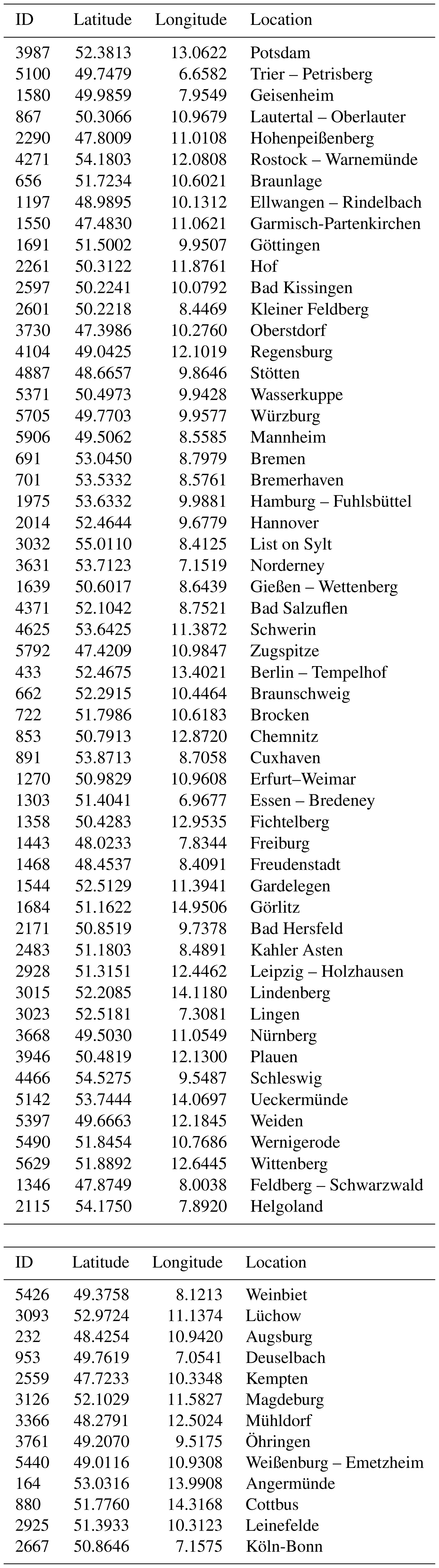
Table A2 Location trend results for the hourly temperature time series. p_{MEAN DIFF} H_A: μ_1960–1990<μ_1991–2018 and p_MK H_A: trend.

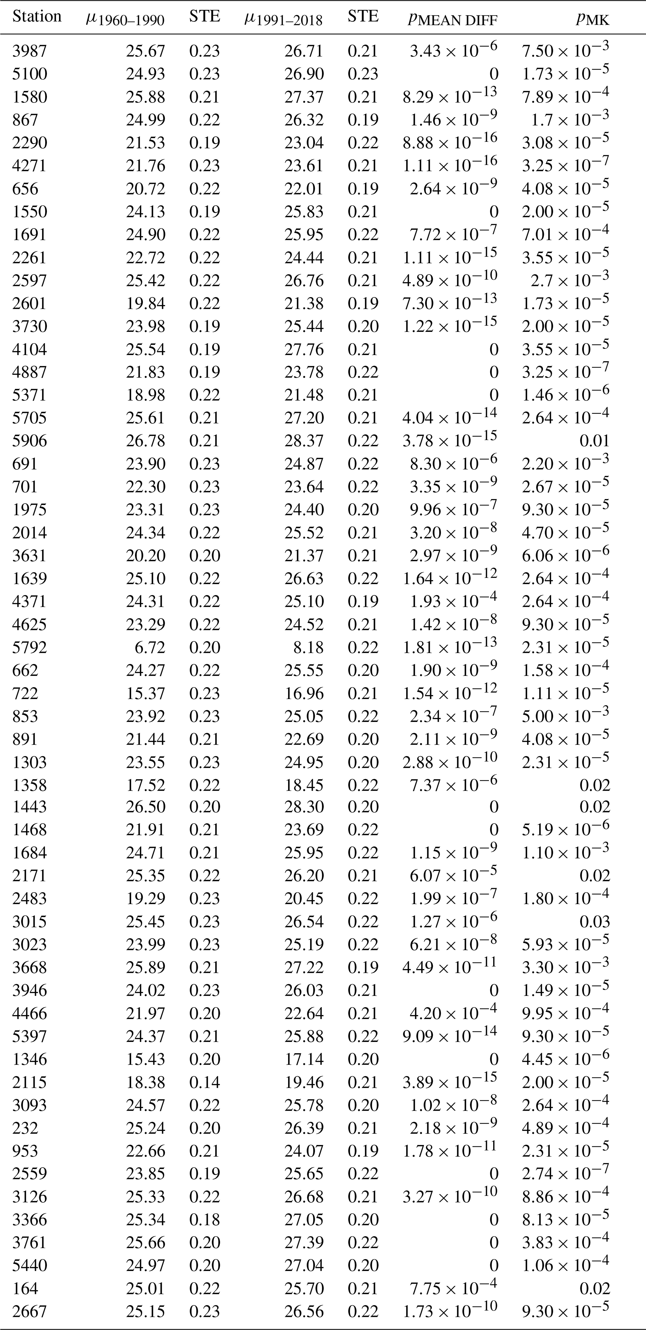
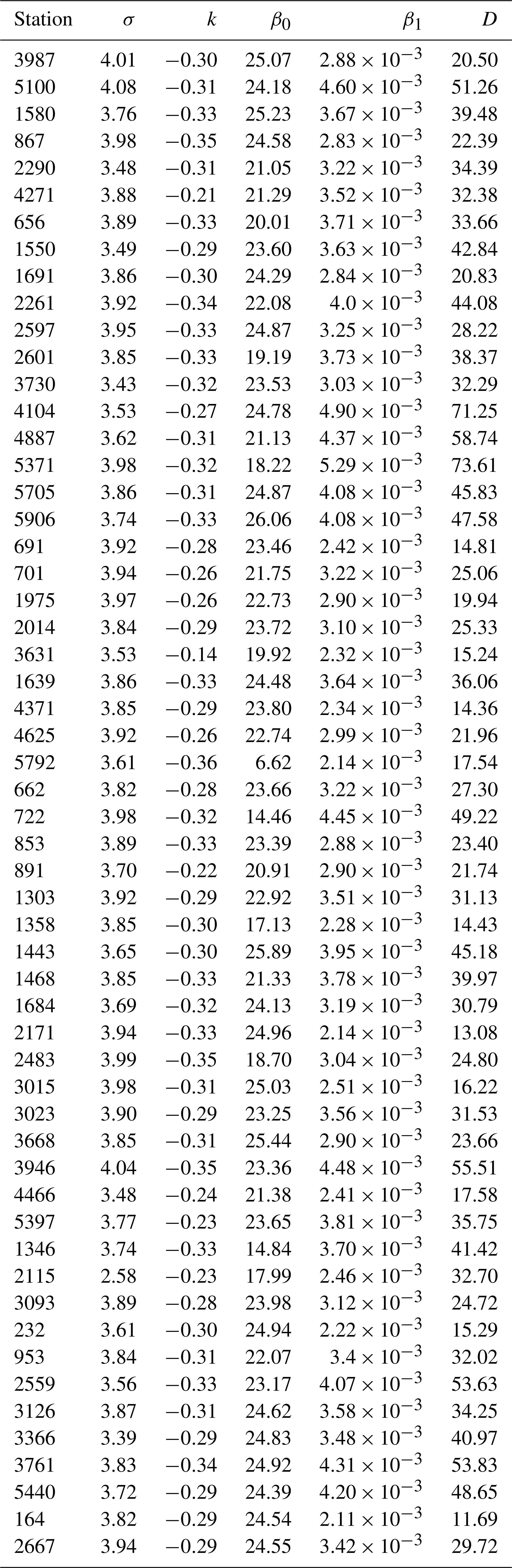
Table A3 MLE nonstationary models for temperature maxima. scale σ, shape k, location $\mathit{\mu }\left(t\right)={\mathit{\beta }}_{\mathrm{0}}+{\mathit{\beta }}_{\mathrm{1}}\times t$, and likelihood D parameters. Here, t is 1 week.