the Creative Commons Attribution 4.0 License.
the Creative Commons Attribution 4.0 License.
 | 23 Jul 2020
A statistical approach to fast nowcasting of lightning potential fields
Joshua North
Zofia Stanley
William Kleiber
Wiebke Deierling
Eric Gilleland
Matthias Steiner
Thunderstorms and associated hazards like lightning can pose a serious threat to people outside and infrastructure. Thus, very short-term prediction capabilities (called nowcasting) have been developed to capture this threat and aid in decision-making on when to bring people inside for safety reasons. The atmospheric research and operational communities have been developing and using nowcasting methods for decades, but most methods do not rely on formal statistical approaches. A novel and fast statistical approach to nowcasting of lightning threats is presented here that builds upon an integro-difference modeling framework. Inspiration from the heat equation is used to define a redistribution kernel, and a simple linear advection scheme is shown to work well for the lightning prediction example. The model takes only seconds to estimate and nowcast and is competitive with a more complex image deformation approach that is computationally infeasible for very short-term nowcasts.
- Article
(3991 KB) - Full-text XML
- BibTeX
- EndNote


Convective storms can pose a significant threat to people and infrastructure as a result of hazardous lightning strikes, hail, heavy precipitation, strong winds, and possible tornadoes. Because of this threat, very short-term forecasting capabilities (termed nowcasting) have been developed to monitor a current situation and predict it up to a few hours into the future (e.g., Wang et al., 2017). Most of these nowcasting techniques rely on empirical methods that use observations made by radar and satellite and short-term numerical model output to capture the initiation, growth, and decay of thunderstorms. The starting point is to identify existing storms (in all of their phases) and then extrapolate their position and evolution based on recent trends in storm evolution and motion. The extrapolation of the position of storms is done with algorithms such as TITAN (Dixon and Wiener, 1993; Han et al., 2009) or the storm cell identification and tracking (SCIT) algorithm (e.g., Johnson et al., 1998). Pierce et al. (2012) provide an excellent review of the nowcasting history and techniques, including both heuristic and numerical weather prediction (NWP) approaches. Joe et al. (2012) elaborate on radar as a key tool for nowcasting of severe weather and discuss state-of-the-art nowcasting systems around the world. Nowcasting techniques are pretty mature and widely utilized by weather services and private vendors to alert the public of imminent threats. More tailored solutions may be offered by vendors to support decision-making for specialized applications.
Monitoring of thunderstorms and lightning is essential for personnel safety at airports where staff servicing the aircraft are exposed to the weather and are possibly in harm's way. Therefore, major airports employ lightning safety procedures to bring outdoor personnel inside to safety when lightning is an imminent threat. These safety procedures, however, result in a temporary halt of the serving of the aircraft and thus may incur schedule delays, especially if these stoppages are numerous or prolonged (Steiner et al., 2013, 2014, 2016). These lightning alert systems range from direct lightning observations and simple heuristics to fully automated and sophisticated thunderstorm hazard warning systems, such as those deployed at the Hong Kong International Airport (Li and Lau, 2008).
Lightning prediction some time into the future is rather challenging, as it depends on how a thunderstorm evolves in time and especially how its kinematics and microphysical processes enable cloud electrification and charge separation that ultimately may result in lightning. Heuristic techniques have been developed to capture thunderstorm electrification and the potential for lightning to occur. There are also fully explicit numerical prediction models that attempt to represent what is going on inside a thunderstorm, including the electrification processes; however, this requires substantial computational resources. The lightning potential prediction is further discussed in Sect. 1.1. Overall, lightning prediction carries notable uncertainty and is thus often approached in terms of probabilistic prediction.
Incorporating uncertainty into forecasts is important for decision-making processes (Steiner et al., 2010; Kicinger et al., 2016). Most nowcasting models are deterministic, although some authors have begun considering modeling uncertainty using combined NWP with remote sensing data (Mecikalski et al., 2015). Only in the past decade or so have statisticians taken an interest in developing model-based nowcasts (Fox and Wikle, 2005; Xu et al., 2005; Metta et al., 2009). However, these initial proposals were relatively complex spatiotemporal Bayesian hierarchical models which are not necessarily suitable for large datasets and real-time applications. For example, modern radar imagery from which nowcasts can be derived is often high dimensional; in the example below, nowcasting of 5 min lightning potential data at 160 000 spatial locations are considered, where simple statistical approaches are required for computational feasibility.
Here, we propose a statistical approach for nowcasting of lightning potential fields. The basic model builds on an integro-difference equation but two important adaptations to that model are made; first, a simple advection function that serves to spatially propagate the storm over the study region and, second, a heat equation model for the redistribution kernel that incorporates both diffusion and source terms. Other authors have considered a continuity equation in the nowcasting contexts (Ruzanski et al., 2011). Critically, the proposed model is very fast to estimate the nowcast (less than 6 s for the example data) and can instantaneously generate forecasts that are validated up to 50 min ahead. The proposed model is compared against a competing, more flexible, but computationally intensive image deformation approach (Aberg et al., 2005). We only compare the proposed method to the image deformation approach for three reasons: first, other nowcasting schemes are not built specifically for lightning potential (Mosier et al., 2011); second, they utilize auxiliary radar information, such as multiple reflectivity values (Han et al., 2009), that is not present in our lightning potential data; and finally, we believe the image deformation approach of Aberg et al. (2005) to be a good representation of modern nowcasting standards. It is found that the predictive ability of the proposed model is generally favorable and substantially faster to estimate the nowcast than the deformation approach. Both models are illustrated on a high-resolution lightning potential dataset and also compared against a persistence forecast.
1.1 Lightning potential and nowcasting
Lightning discharges are the result of storm electric fields generated by kinematic and microphysical processes. The exact details of the relevant processes remain to be fully understood, but substantial observational, laboratory, and modeling evidence suggests that a strong updraft in the mixed-phase region is needed for thunderstorm electrification to result in lightning (Workman and Reynolds, 1949; Williams and Lhermitte, 1983; Zipser and Lutz, 1994; Mansell et al., 2005; Deierling and Petersen, 2008; Deierling et al., 2008). Lightning nowcasting systems often rely on proxy observations that relate to electrification processes to infer lightning. Operational guidance of potential lightning threats makes use of real-time lightning detection and lightning nowcasting systems. A variety of approaches on nowcasting lightning exist. These are either based on a single parameter or a combination of several parameters. In the following, commonly used approaches and parameters are briefly described.
Electric field mills measure the vertical component of electric fields overhead and provide direct measurements of integrated electric fields from nearby electrified clouds. They monitor the buildup and decay of these fields in storms. As such, electric field mill measurements are used to issue lightning warnings when the electric field measurements exceed a chosen threshold (Murphy et al., 2008). However, such thresholds may not necessarily represent a unique lightning threat. This is because electric field mills measure the integrated vertical component of the electric field from not necessarily just one source but different sources, including all nearby electrified clouds which may be at different stages in their lifetime and have different electric field structures and distances to the field mill. Another way to provide warnings of cloud-to-ground lightning specifically is based on total (in-cloud and cloud-to-ground) measurements. Typically (but not always) in-cloud (IC) lightning precedes cloud-to-ground lightning in a developing storm by several minutes (MacGorman et al., 2011). Thus, some techniques base their warnings on IC lightning activity (Murphy et al., 2002; Holle et al., 2016). Other warning techniques rely on relationships between storm properties and lightning production. In addition they may track these storm properties by making use of nowcasting techniques that predict the initiation, growth, decay and movement of storms.
Many observational studies have shown the radar- or satellite-derived ice content of a cloud to correlate well with lightning production. For example, Buechler and Goodman (1990) found 40 dBZ of radar reflectivity above the −40 C level to be a good indicator for lightning. More recent techniques employ tracking algorithms to follow satellite- or radar-derived glaciation properties of a cloud to predict lightning (Saxen et al., 2008; Potts, 2009; Harris et al., 2010; Mosier et al., 2011). Generally, key parameters that are considered in lightning nowcasting include the following:
-
Various thermodynamic and kinematic indices (e.g., CAPE and lifted index) indicative of the probability of deep convection obtained from soundings, radiometers, or numerical models.
-
Temperature information from soundings, radiometers, or numerical models to identify the ice phase.
-
Ice microphysical parameters derived from radar or passive microwave data, which may include particle type, volumetric ice type information, and their trends, etc.
-
Convective storm intensity and organization derived from radar, passive microwave, or lightning-tracked features or maxima of certain parameters to indicate initiation or growth trends, embedded convection, persistence of features, etc.
-
Storm updraft strength (e.g., updraft volume, maximum updraft speed, or echo top height) from single or multiple Doppler analyses to indicate storm intensity.
Prediction systems are either based on one or a combination of these parameters using a decision tree, fuzzy logic approaches, or NWP models. Prediction systems may also make use of recent numerical model output to predict lightning (Barthe et al., 2010) or use the model output of predicted lightning from explicit electrification and lightning schemes (Mansell et al., 2005; Fierro et al., 2013). Finally, lightning climatologies are also sometimes used to give guidance for lightning occurrence.
Here we use the current National Center for Atmospheric Research (NCAR) lightning nowcasting approach which makes use of observed lightning data such as data from a regional high-precision, high-detection-efficiency Lightning Mapping Array (LMA; Thomas et al., 2004). It also includes relevant storm information derived from volumetric radar and sounding data, such as intensity, organization, and motion, and builds on a fuzzy logic approach that relates radar reflectivity characteristics observed by, for example, the National Weather Service (NWS) Weather Surveillance Radar – 1988 Doppler to lightning potential forecasts (Saxen et al., 2008; Deierling et al., 2014). Based on a careful selection process, a combination of lightning predictor fields was developed to capture lightning from all phases of thunderstorm evolution (i.e., initiation, mature cores, and anvil). The lightning potential output field (e.g., Fig. 1) enables defining areas of higher lightning frequency and probability (pink areas; lightning produced within storm cores) and areas of less likely but still possible lightning (yellow; e.g., lightning produced within anvil clouds). The output is scaled between 0 and 1.6 where areas of lower lightning potential thresholds (∼0.1–0.8 lightning potential values) are associated with storm anvils and storm initiation (yellow areas in Fig. 1). Areas of higher lightning potential thresholds (>0.8 lightning potential values) are related to lightning in thunderstorm cores (pink areas in Fig. 1). Using tunable thresholds the lightning potential nowcasts can be adapted to reflect specific user needs (e.g., lower thresholds yield longer lightning alert lead time, longer operational downtimes, but increased safety).
The nowcast lightning potential field is then cast within the mathematical framework laid down by Xu et al. (2005). The major differences in the present proposal are (a) the adoption of a physical argument for a new redistribution kernel and (b) a frequentist implementation that generates fast nowcasts for very large datasets.
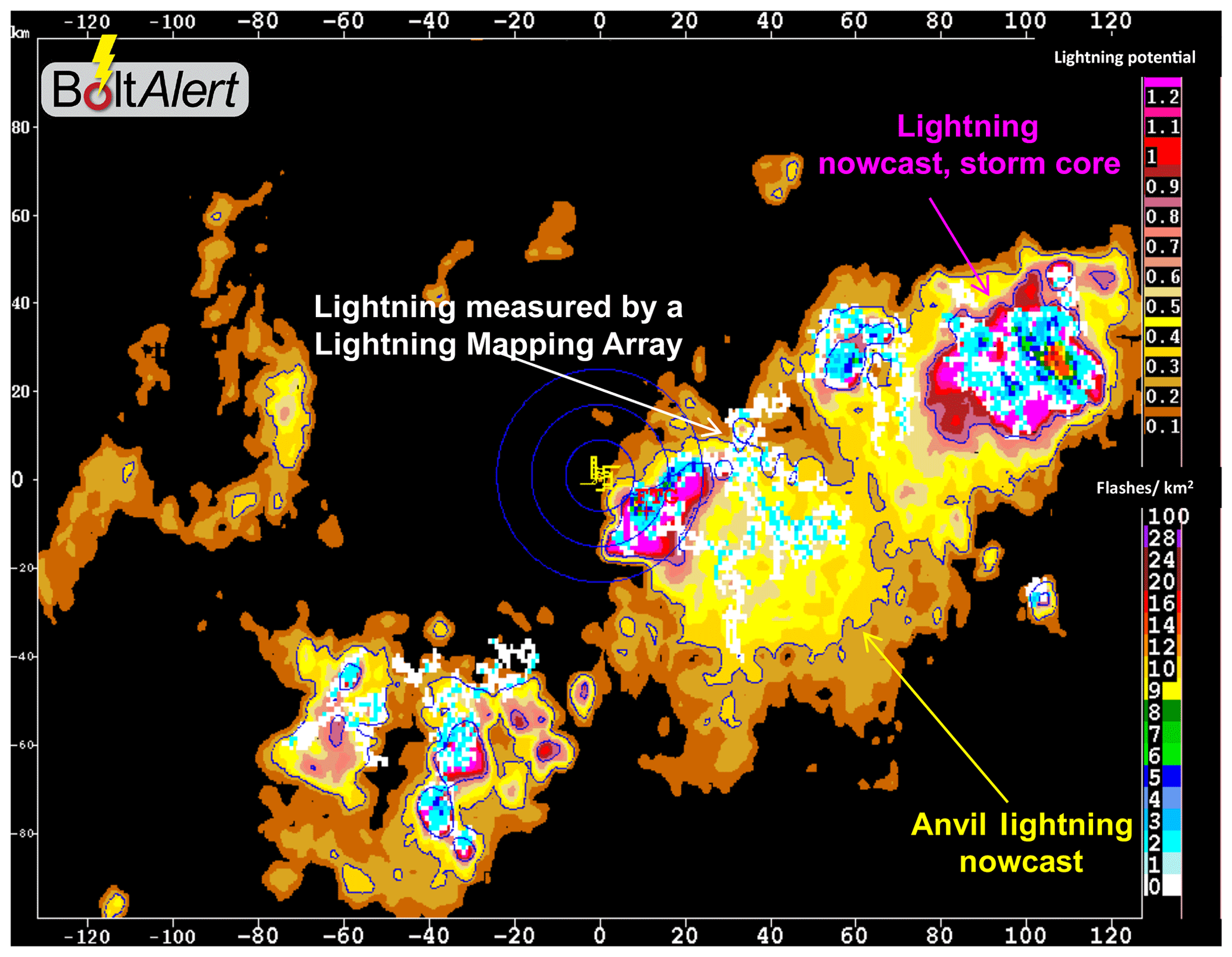
Figure 1Example of a lightning potential nowcast from the enhanced lightning prediction capability that includes storm cores (magenta shading) and anvil (yellow shading), with contemporaneous Lightning Mapping Array (LMA) data overlaid. Two color scales are shown to the right. The upper scale is for the lightning potential, with warmer colors showing the higher potential for lightning to occur. The lower scale is for the lightning flash extent (i.e., horizontal footprint) as depicted by the LMA.
2.1 A statistical nowcasting framework
Consider a space–time field of lightning potentials in which over a spatial domain at a set of time points . The goal in a nowcasting situation is, given observations , to predict for relatively small k≥1, i.e., a few time steps ahead. In general, throughout this section, an observed image is denoted by and a forecast field valid at time t+k on 𝒟 is denoted by . The one-step-ahead forecast field is assumed to follow an integro-difference equation representation as follows:
Here, is the forecast image at the new time t+1, given the most recent image . The function k(s,u) is a real valued redistribution kernel that serves to advect and redistribute the image into the future. The function is an advection kernel and serves to spatially propagate the storm.
The integro-difference equation (Eq. 1) produces one-step-ahead forecasts; one approach to producing multiple-step-ahead forecasts is to iteratively apply Eq. (1). For example, a two-step-ahead forecast can be defined by the following:
The key decisions in this framework are in specifying the redistribution kernel k and the advection function S, which are taken up next.
2.1.1 The advection function
Xu et al. (2005) use a redistribution kernel that is a weighted combination of orthonormal spectral basis functions. This choice introduces a large number of coefficient parameters that must be constrained somehow. The approach proposed here is to separately parameterize the advection, diffusion, and convection processes.
One of the basic assumptions is that, on very short timescales, storms advect almost linearly, which is certainly not true over longer periods of time (e.g., half hourly intervals). However, the focus study of 5 min lightning potential snapshots operates under this assumption. Thus, the rigid spatial deformation function is as follows:
where and T denotes the transpose operation. Here, , and βy are statistical parameters, and εx(t) and εy(t) are Gaussian white noise processes. This structure assumes a time-constant advection at rate αx and αy, with possible linear acceleration βx and βy. Splitting these functions across directions allows for distinct cardinal direction movements. Using such an advection function within an integro-difference equation such as Eq. (1) allows for extradiffusive propagation, which results from displacing the kernel relative to a fixed spatial location (Xu et al., 2005).
2.1.2 The redistribution kernel
The proposal for the redistribution kernel is inspired by a model from physics, namely the heat equation. The heat equation is a partial differential equation that describes how the distribution of heat (or, in this case, lightning potential) changes in time with respect to the local spatial curvature of heat. The heat equation is described briefly and a numerical approximation to its solution is related to the integro-difference equation Eq. (1).
The 2D heat equation is as follows:
In this version of the heat equation, Q(s,t) acts as a convection term, which can increase the local rate of change of lightning potential, while the first terms are spatial diffusions whose strength is modulated by the diffusivity coefficient α. Note that in the applied mathematics literature, convection and advection are often used interchangeably. The source term Q(s,t) is referred to as a convective source because of a typical phenomenon of intense lightning generating thunderstorms occurring caused by convective vertical air movements that enhance such activity.
Given boundary conditions and the source term Q(s,t), Eq. (3) defines a function f at all spatial locations and time points. The key assumption is that over very short timescales, lightning potential fields approximately evolve according to Eq. (3), but the solution updates according to new radar imagery. In particular, consider a finite difference approximation to the solution to Eq. (3), as follows:
where Δt is a small time step, h is a northing or easting spacing (which is assumed, here, to be equal), and and e1 and e2 are the Euclidean basis vectors in ℝ2. The approximation in Eq. (4) can be calculated on the interior of 𝒟; boundary solutions use appropriate forward or backward approximations. For the example dataset, h=1, Δt=0.16, and α=1; these choices are related to the Courant–Friedrichs–Lewy condition of the heat equation, which essentially states that a small enough time stepping is required so that the numerically approximated solution is stable. The parameter r could be estimated in a constrained estimation framework, but it has been found that these choices work very well for the application below.
Now it can be seen how Eq. (4) defines the kernel function of Eq. (1). In particular, the finite sum version of Eq. (1) is the following:
The presence of the convective term in k results in a nonstationary redistribution kernel, which gives substantially more flexibility in locally diffusing or concentrating the forecast images.
2.2 Image deformation: nowcasting approach
In a realistic nowcasting scenario there is not time to fit a large, complicated Bayesian hierarchical statistical model such as those defined in Xu et al. (2005) or Fox and Wikle (2005; e.g., the dataset here is more than 140 times larger than those considered by these authors). Thus, a comparison against a competing approach that comes from the image deformation literature is applied, namely an adaptation of the model proposed by Aberg et al. (2005), which is expected to exhibit greater flexibility but at the cost of increased computation.
The deformation-based forecast is as follows:
where is a temporally indexed spatial deformation function. One of the most common deformation functions is a pair of thin plate splines (Bookstein, 1989; Gilleland et al., 2010, 2011) is the following:
for , where U(r)=r2log r for r>0 is a radial basis function and {uj}⊂𝒟 form a set of knots on the nowcasting domain. The parameters serve to allow for nonlinear transformations in the spatial domain. This class of deformations can result in space folding over upon itself and requires some regularization, which is typically enforced during the estimation step.
The parameters are estimated by minimizing a penalized mean squared error based on the bending energy of a thin plate spline. For the lightning potential nowcasting example the deformation parameters are estimated by minimizing the following:
where 𝒫 is the bending energy of a thin plate spline (see Gilleland et al. (2011) for details). The second term controls the amount of allowed deformation, and λ≥0 is a smoothing parameter. Then, the one-step-ahead forecast is , and multiple-step-ahead forecasts can be generated by recursively applying the deformation, for example, . Given a new observed potential field at t+1, the deformation function is reestimated by comparing time points t and t+1.

Figure 2Mean squared errors and estimation time for training the deformation model on a pair of images.
The application, here, is in forecasting lightning potential. Lightning potential is an indication of how likely it is to have a lightning strike in an area. It is not a probability in that it is not constrained to be in the interval [0,1] but serves as a surrogate for a probability. Our data are over a 400 km × 400 km area, which are descritized to a 400×400 grid, available at 5 min snapshots for a period of a little over 6 h.
A complicated dynamic space–time dataset such as the one considered in this study could beckon a complicated and comprehensive estimation framework that accounts for various sources of uncertainty. However, as the goal is to produce nowcasted forecast fields almost instantaneously, simple estimation approaches must be used.
3.1 Estimation of the proposed statistical model
The statistical parameters of the model are those in the advection function and the convective source function Q(s,t). Given Q(s,t), a simple mean squared error criterion is used as the loss function to estimate an optimal advection function for a given time step and the averages are taken over all spatial locations. The estimation and forecasting algorithm is as follows:
-
At time point t, given observed lightning potential field , estimate S(s,t) numerically by minimizing , resulting in .
-
Given estimates for , fit advection parameters of Eq. (2) by ordinary least squares.
-
Use the conditional mean of from its predictive distribution, given parameters estimated in the previous step.
-
Approximate the solution to Eq. (1) to generate a forecast field .
-
Multiple-step-ahead forecasts are generated by recursive applications of Eq. (1).
All that remains is the choice of, or estimate of, Q(s,t). The following model is proposed: , where F0(s,t) is the forecast of time t with . In particular, F0 accounts for the advection but not diffusion term. Other models for Q(s,t) were entertained, most notably , but it was found that the proposed Q(s,t) resulted in the lowest mean squared predictive error for the nowcasts. Heuristically, positive values of Q(s,t) indicate locations that are locally experiencing increasing potential, whereas locations with are decreasing in lightning potential and projections into the next time step are made accordingly.
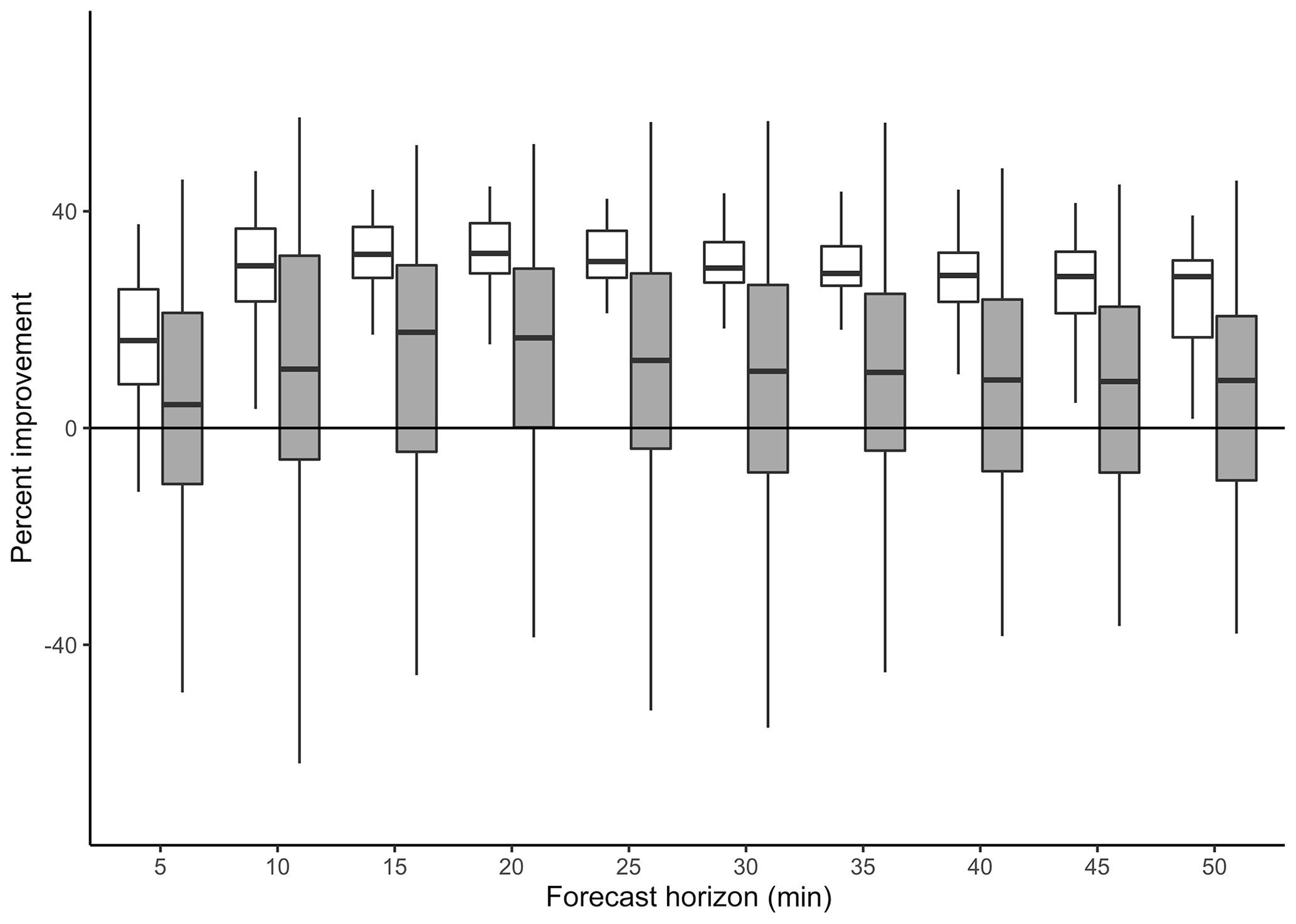
Figure 3Percent improvement in mean squared error over the persistence forecast. Box plots represent the 54 validation times in the dataset for percent improvement using the proposed approach (white) and the deformation approach (gray). Outliers have been removed.
To find r and γ we implement a small experiment. In particular, we perform grid searches over and , where values of γ−1 above 500 show negligible differences. Using a subset of data, namely every fifth image, we calculate mean squared error averaged over all one-time-step-ahead nowcasts. Predictive results were optimized at and r=0.15, which we fix for the ensuing discussion. We recognize that r and γ could be included in the estimation process but, based on the time they took to optimize offline, the computational cost was not worth it.
3.2 Estimation of the deformation function
The two crucial quantities in the deformation approach are knot locations (sometimes called landmark or control points) and the smoothing parameter λ. Heuristically, the more knots used, the greater the flexibility of deformation. However, a high number of knots introduces many statistical parameters bij, and numerical optimization of the penalized log likelihood becomes prohibitive, especially in a nowcasting context.

Figure 4Easting and northing estimates of advection function S with a linear fit. The linear increase suggests the study storm is accelerating in the northeasterly direction.
The number of knots, therefore, is chosen to be 100 (placed on a 10×10 evenly spaced grid) determined through experimentation. In particular, we consider the following experiment: using image pairs at times t and t+1, we deform time point t's image with evenly spaced grids of L2 knots for with and compare to t+1 for t=17. We calculate the mean squared error (MSE) over all possible deformations. The results are plotted in Fig. 2. Clear improvements in MSE are apparent until approximately 100 knots are in the model. The further reduction beyond 400 points may be the result of overfitting. Note that other trial time periods resulted in similar reductions in MSE. As a second consideration, Fig. 2 also shows the computational time required to estimate the deformation under these experimental conditions as a function of number of knots. When we calculate the deformation going forward, we warm start the optimization, described below, which significantly reduces the computational time. Therefore, the timing in Fig. 2 is not reflective of the actual time it takes to calculate a single deformation. Nonetheless, this experiment is valuable because it informs our decision of the number of landmark points to choose. Clearly there is a trade-off between complexity and model fit; given the stabilization of MSE and increase in computation time beyond, we opt for 100 knots going forward.
The smoothing parameter λ is chosen to be fixed at 103 after experimentation. In particular, using the same pair of training points as for the knot placements, deformations are tested under penalties with λ varying from 10−10 to 105. MSEs (not shown) are effectively unchanged based on different λs but with a slight improvement around 103 in the third decimal. The lack of impact of λ is likely caused by adjacent time points exhibiting small spatial changes, whereas λ is known to be more important for scenarios when target and training images exhibit substantial differences (Gilleland et al., 2011).
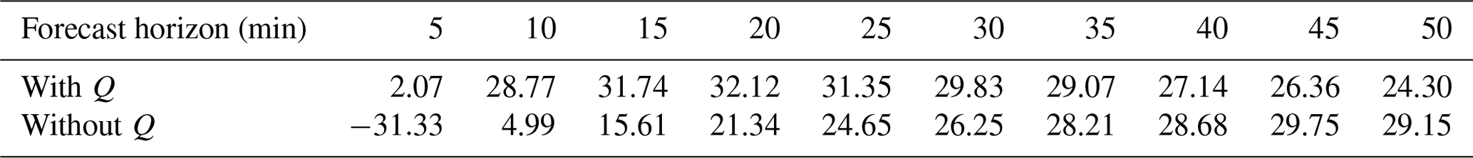
Table 1Average percentage improvement in mean squared prediction error over the persistence forecast for the nowcasting model with and without Q(s,t).
Operationally, we see that adjacent time warps exhibit substantial large-scale similarities, associated with dominant weather patterns. Therefore, we warm started the optimization using previous optimization results for all but the first warp. This substantially decreases the computational time associated with estimating the warp. For the first warp a warm start is not possible and, rather than fitting all deformation parameters simultaneously, we adopted an iterative approach. In particular, with 100 knots there are more than 100 statistical parameters, which precludes feasible estimation. Thus, the strategy, here, is as follows: for a given training pair of fields the optimal deformation is first estimated with 22 knots. The estimated deformation is then used as initial conditions for 32 evenly spaced knots, and this procedure is applied iteratively for L2 points with . The final set of points is then fixed and used in the nowcasting step.
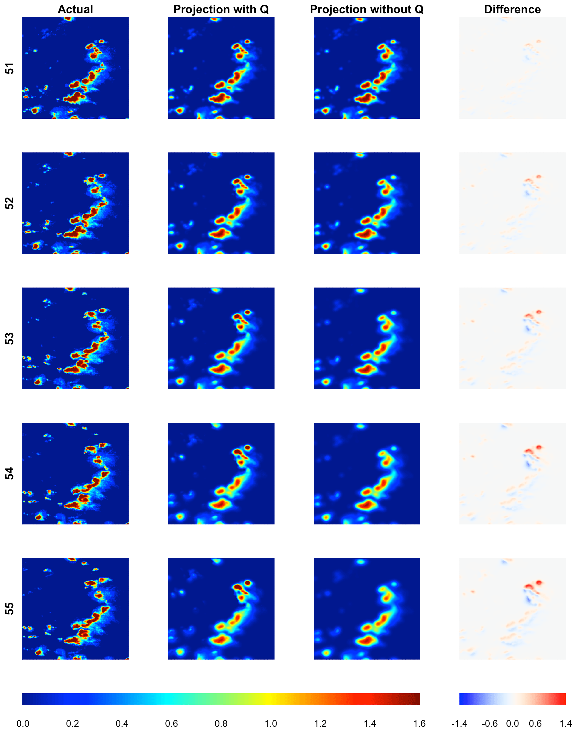
Figure 5Observed and nowcasted fields of lightning potential using the proposed approach that includes Q(s,t) and without Q(s,t) for forecast horizons 5 min to 25 min, validating at time steps 51–55. The far right column depicts the difference of the nowcasted field that includes Q(s,t) subtracted from the nowcasted field without Q(s,t). The left legend corresponds to the lightning potential, and the right legend corresponds to the difference in lightning potential from the projection with Q and the projection without Q.
The proposed statistical model is compared against competitors including a persistence forecast, i.e., which uses the most recently available observed image as the future forecast for all lead times, and the deformation approach of Sect. 2.2. Deformation-based nowcasts rely on optimizing the single-step deformation with recursive applications of the warp to generate future lead time forecasts.
Before illustrating the predictive ability of both models, we note differences in computational costs. Nowcasting under any of the three approaches is essentially instantaneous, but the primary computational bottleneck is in estimating the appropriate statistical parameters based on historical images. For example, on the same laptop computer, the average time required to estimate a deformation field with a warm start is about 2 m 22 s, while the proposed statistical model averages less than 6 s to estimate the nowcast. Crucially, this result implies that computation is prohibitive for the deformation approach to work for very short-term nowcasts, while the new model is easy to implement and estimate.
For the deformation and proposed nowcasts, the deformed/shifted images will propagate outside of the domain of interest. Observed pixels that are shifted outside of the domain are ignored and unavailable field values that are brought into the domain are set to be zero, reflecting the assumption that the majority of active potentials are in the interior of the forecast domain. No field buffer is used in calculating the validation statistics below.
4.1 Comparison to deformation and persistence
To test the feasibility of the proposed method, a comparison against both deformation and persistence is made. Figure 3 shows box plots of percentage improvements in mean squared error (MSE) of the nowcasts over the persistence forecast for horizons 5 min to 50 min ahead. MSEs are calculated as pointwise squared differences averaged throughout the model domain. The box plots represent 54 forecast comparisons in which we begin forecasting the fourth time point, using the first three images for training only. White box plots represent the proposed approach, while gray box plots represent deformation.
Noticeable patterns are apparent; there is substantially more variability in the deformation-based approach than the proposed statistical model. This result is likely caused by the increased degrees of freedom allowed with the deformation model, which sometimes results in better forecasts than proposed model but can also often result in forecasts worse than persistence. Both methods improve on persistence out to about a 25 min lead time. Deformation then experiences a slight decay in predictive improvement but, on average, still improves over persistence even at the longest lead times. The proposed method's improvement seems more stable both in terms of having less variability but also in maintaining consistent improvement over persistence out to the longest horizon at more than 25 % improvement. Overall, the proposed method outperforms deformation in 86 % of validation times. Note that outliers have been removed from this plot for readability.

Figure 6Observed and nowcasted fields of lightning potential. The first column shows observed potential fields at five time points. Each ensuing column is a projection of the observed starting at time points 50, 51, 52, and 53, respectively. The legend corresponds to the lightning potential.
4.2 Importance of S(s,t)
In the next two subsections, we take a closer look at two components of the proposed model, namely the advection function and the convection or generation function. First, the importance of the advection function, S(s,t), is considered. This function serves to spatially propagate the current image into the future. Figure 4 shows the estimated advection components of S at each time point with a fitted linear trend in both the easting and northing directions. There is an apparent approximate linear increase over the course of the storm in both components, suggesting a northeasterly acceleration of the storm. The linear statistical model for S in Eq. (2) is tailored to this particular storm but, for a short time frame, nowcasting seems a reasonable model unless there is evidence of acceleration. Both Figs. 3 and 4 suggest that the advection function is an important component of the nowcasting model. An autoregressive model, i.e., AR(1), specification for the errors from the fitted linear model to predict future movement was also investigated, but no statistically significant improvement in predictive ability was found. We also examined the potential correlation between the easting and northing component linear model errors, and while there is evidence of correlation with , we do not currently use this information as we do not simulate from the predictive distribution of S but rather use its predictive mean. To generate an ensemble of forecasts, it would be natural to model the errors as a bivariate white noise Gaussian process.
4.3 Importance of Q(s,t)
The convection or generation matrix Q(s,t) is a crucial element of the model which allows for focused areas of increasing lightning potential but also areas of diminishment. The model used here for Q is a scaled difference between the current time step image and the forecast of the current time step's image, which in principle represents areas of instantaneous lightning potential generation and decay. Areas that grew over the previous time step are projected to continue growth into the future and areas that abate will continue to do so.
To motivate the importance of Q in the model, we compare relative improvements in the mean squared error of the nowcasted fields over the persistence forecast using the proposed model with, and without, Q. Table 1 shows average improvement for forecast horizons of 5 min to 50 min. Improvements are calculated as an average percent improvement over persistence in forecast mean squared error (MSE) over the 54 validation times. The importance of Q is clear, with a 15 %–30 % reduction in relative MSE over the model without Q at shorter lead times, which turns negligible at longer lead times.
Figure 5 visually assesses the importance of including Q(s,t) in the nowcasting setup. It contains forecast horizons for lead times of 5 min to 25 min using the proposed nowcasting approach with, and without, Q to validate time points 51–55. Throughout we use the fitted regression line for . At the shortest lead time there is not much apparent difference between both models, but the difference becomes notable at longer lead times. For instance, in the final row of Fig. 5, the forecast using Q exhibits much stronger concentrations of lightning potential in the north central region, while the forecast without Q has allowed the field strength in these areas to incorrectly wane.
This verification section is closed with a final example of nowcasted fields under the currently proposed model. Figure 6 shows observed potential fields for time points 51–55. The next columns show nowcasted fields that initialize from time point 50 (second column) to 53 (final column). The northeastward propagation of the storm is apparent in both the observed imagery and also the nowcasted fields because of the advection function. As in the previous Figure, the Q function serves to ensure the forecasts maintain higher potential values in areas of intense lightning activity.
In this paper, a simple but fast method is proposed for nowcasting of lightning potential fields. Nowcasts are defined through the solution to an integro-difference equation that includes a nonstationary redistribution kernel. The redistribution kernel allows for advection, diffusion, and concentration or convection of lightning potentials and is thus a flexible model for short-term propagation of lightning potential imagery into the future.
However, sensitive parameterizations are necessary to make both estimation and forecasting feasible for operational applications. We propose simple parameterizations of the advection and convection functions and allow the redistribution kernel to be approximated by a numerical solution of the heat equation. Results from test cases suggest that the proposed formulation provides substantially better short-term forecasts over the persistence forecast. Also, over such short timescales, linear advection performs as well as more complicated nonlinear deformation-based forecasts and is orders of magnitude faster in computation time.
A number of future research routes seem clear. Comprehensive quantification of uncertainty is an important but delicate problem; sources of uncertainty include those parameters in the advection function, and choice of the convection function Q. However, for very large datasets, care must be taken in a parameterization that allows for flexibility but also ensures very fast estimation or approximation. Moreover, how to communicate uncertainty in a nowcasting context seems of particular concern.
Code can be found on Joshua North's GitHub page at https://github.com/jsnowynorth/nowcasting (North, 2020).
Data are available upon request from the authors.
JN developed the new nowcasting code and heat equation implementation. ZS implemented the deformation approach. WK assisted with model development and provided expertise on deformation. WD provided data and expertise on lightning potential and nowcasting. EG provided code and expertise on deformation. MS provided expertise on nowcasting. All authors edited and wrote portions of the paper.
The authors declare that they have no conflict of interest.
Any opinions, findings, and conclusions or recommendations expressed in this paper are those of the authors and do not necessarily reflect the views of the funding agencies.
William Kleiber's portion of the research was funded by the National Science Foundation (NSF; grant nos. DMS-1811294 and DMS-1923062). The National Center for Atmospheric Research (NCAR) is funded by the NSF. The lightning potential work was partly funded by NSF, the United States Army Test and Evaluation Command (ATEC), and the Federal Aviation Administration (FAA).
This research has been supported by the National Science Foundation, Division of Mathematical Sciences (grant nos. 1811294 and 1923062).
This paper was edited by Dan Cooley and reviewed by two anonymous referees.
Aberg, S., Lindgren, F., Malmberg, A., Holst, J., and Holst, U.: An image warping approach to spatio-temporal modelling, Environmetrics, 16, 833–848, 2005. a, b, c
Barthe, C., Deierling, W., and Barth, M. C.: Estimation of total lightning from various storm parameters: A cloud-resolving model study, J. Geophys. Res.-Atmos., 115, D24202, https://doi.org/10.1029/2010JD014405, 2010. a
Bookstein, F. L.: Principal warps: Thin-plate splines and the decomposition of deformations, IEEE T. Pattern Anal., 11, 567–585, 1989. a
Buechler, D. E. and Goodman, S. J.: Echo size and asymmetry: Impact on NEXRAD storm identification, J. Appl. Meteorol., 29, 962–969, 1990. a
Deierling, W. and Petersen, W. A.: Total lightning activity as an indicator of updraft characteristics, J. Geophys. Res.-Atmos., 113, D16210, https://doi.org/10.1029/2007JD009598, 2008. a
Deierling, W., Petersen, W. A., Latham, J., Ellis, S., and Christian, H. J.: The relationship between lightning activity and ice fluxes in thunderstorms, J. Geophys. Res.-Atmos., 113, D15210, https://doi.org/10.1029/2007JD009700, 2008. a
Deierling, W., Steiner, M., Ikeda, K., Kessinger, C., and Bass, R.: Short term lightning hazard predictions, in: XV International Conference on Atmospheric Electricity, Norman, OK, 2014. a
Dixon, M. and Wiener, G.: TITAN: Thunderstorm identification, tracking, analysis, and nowcasting – A radar-based methodology, J. Atmos. Ocean. Technol., 10, 785–797, 1993. a
Fierro, A. O., Mansell, E. R., MacGorman, D. R., and Ziegler, C. L.: The implementation of an explicit charging and discharge lightning scheme within the WRF-ARW model: Benchmark simulations of a continental squall line, a tropical cyclone, and a winter storm, Mon. Weather Rev., 141, 2390–2415, 2013. a
Fox, N. I. and Wikle, C. K.: A Bayesian quantitative precipitation nowcast scheme, Weather Forecast., 20, 264–275, 2005. a, b, c
Gilleland, E., Lindström, J., and Lindgren, F.: Analyzing the image warp forecast verification method on precipitation fields from the ICP, Weather Forecast., 25, 1249–1262, 2010. a
Gilleland, E., Chen, L., DePersio, M., Do, G., Eilertson, K., Jin, Y., Kang, E., Lindgren, F., Lindström, J., Smith, R., and Xia, C.: Spatial forecast verification: image warping, Technical Report TN-482+STR, National Center for Atmospheric Research, 2011. a, b, c
Han, L., Fu, S., Zhao, L., Zheng, Y., Wang, H., and Lin, Y.: 3D convective storm identification, tracking, and forecasting – An enhanced TITAN algorithm, J. Atmos. Ocean. Technol., 26, 719–732, 2009. a, b
Harris, R. J., Mecikalski, J. R., MacKenzie Jr., W. M., Durkee, P. A., and Nielsen, K. E.: The definition of GOES infrared lightning initiation interest fields, J. Appl. Meteorol. Climatol., 49, 2527–2543, 2010. a
Holle, R. L., Demetriades, N. W., and Nag, A.: Objective airport warnings over small areas using NLDN cloud and cloud-to-ground lightning data, Weather Forecast., 31, 1061–1069, 2016. a
Joe, P., Dance, S., Lakshmanan, V., Heizenreder, D., James, P., Lang, P., Hengstebeck, T., Feng, Y., Li, P. W., Yeung, H.-Y., Suzuki, O., Doi, K., and Dai, J.: Automated Processing of Doppler Radar Data for Severe Weather Warnings, INTECH Open Access Publisher, 2012. a
Johnson, J., MacKeen, P. L., Witt, A., Mitchell, E. D. W., Stumpf, G. J., Eilts, M. D., and Thomas, K. W.: The storm cell identification and tracking algorithm: An enhanced WSR-88D algorithm, Weather Forecast., 13, 263–276, 1998. a
Kicinger, R., Chen, J.-T., Steiner, M., and Pinto, J.: Airport capacity prediction with explicit consideration of weather forecast uncertainty, J. Air Transp., 24, 18–28, 2016. a
Li, P. and Lau, D.: Development of a lightning nowcasting system for Hong Kong International Airport, in: 13th Conference on Aviation, Range and Aerospace Meteorology, New Orleans, Louisiana, USA, 20–24 January, 2008. a
MacGorman, D. R., Apostolakopoulos, I. R., Lund, N. R., Demetriades, N. W., Murphy, M. J., and Krehbiel, P. R.: The timing of cloud-to-ground lightning relative to total lightning activity, Mon. Weather Rev., 139, 3871–3886, 2011. a
Mansell, E. R., MacGorman, D. R., Ziegler, C. L., and Straka, J. M.: Charge structure and lightning sensitivity in a simulated multicell thunderstorm, J. Geophys. Res.-Atmos., 110, D12101, https://doi.org/10.1029/2004JD005287, 2005. a, b
Mecikalski, J. R., Williams, J. K., Jewett, C. P., Ahijevych, D., LeRoy, A., and Walker, J. R.: Probabilistic 0–1-h convective initiation nowcasts that combine geostationary satellite observations and numerical weather prediction model data, J. Appl. Meteorol. Climatol., 54, 1039–1059, 2015. a
Metta, S., von Hardenberg, J., Ferraris, L., Rebora, N., and Provenzale, A.: Precipitation nowcasting by a spectral-based nonlinear stochastic model, J. Hydrometeorol., 10, 1285–1297, 2009. a
Mosier, R. M., Schumacher, C., Orville, R. E., and Carey, L. D.: Radar nowcasting of cloud-to-ground lightning over Houston, Texas, Weather Forecast., 26, 199–212, 2011. a, b
Murphy, M., Demetriades, N., and Cummins, K.: The value of cloud lightning in probabilistic thunderstorm warning, 16th Conf. on Probability and Statistics in the Atmospheric Sciences, American Meteorological Society, Orlando, FL, 134–139, 2002. a
Murphy, M. J., Holle, R. L., and Demetriades, N. W.: Cloud-to-ground lightning warnings using electric field mill and lightning observations, in: 20th international lightning detection conference, Tucson, AZ, 21–23, 2008. a
North, J.: nowcasting, GitHub, available at: https://github.com/jsnowynorth/nowcasting, last access: 19 May 2020. a
Pierce, C., Seed, A., Ballard, S., Simonin, D., and Li, Z.: Nowcasting, in: Doppler Radar Observations-Weather Radar, Wind Profiler, Ionospheric Radar, and Other Advanced Applications, edited by: Bech, J., 2012. a
Potts, R. J.: A thunderstorm and lightning alert service for airport operations, American Meteorological Society, Phoenix, AZ, 12–15, 2009. a
Ruzanski, E., Chandrasekar, V., and Wang, Y.: The CASA nowcasting system, J. Atmos. Ocean. Technol., 28, 640–655, 2011. a
Saxen, T. R., Mueller, C. K., Warner, T. T., Steiner, M., Ellison, E. E., Hatfield, E. W., Betancourt, T. L., Dettling, S. M., and Oien, N. A.: The operational mesogamma-scale analysis and forecast system of the US army test and evaluation command. Part IV: The White Sands Missile Range auto-nowcast system, J. Appl. Meteorol. Climatol., 47, 1123–1139, 2008. a, b
Steiner, M., Bateman, R., Megenhardt, D., Liu, Y., Xu, M., Pocernich, M., and Krozel, J.: Translation of ensemble weather forecasts into probabilistic air traffic capacity impact, Air Traffic Control Quarterly, 18, 229–254, 2010. a
Steiner, M., Deierling, W., and Bass, R.: Balancing safety and efficiency of airport operations under lightning threats: a look inside the race closure decision-making process, Air Traffic Control, 55, 16–23, 2013. a
Steiner, M., Deierling, W., Ikeda, K., and Bass, R. G.: Ground delays from lightning ramp closures and decision uncertainties, Air Traffic Control Quarterly, 22, 223–249, 2014. a
Steiner, M., Deierling, W., Ikeda, K., Robinson, M., Klein, A., Bewley, J., and Bass, R.: Air Traffic Impacts Caused by Lightning Safety Procedures, in: 16th AIAA Aviation Technology, Integration, and Operations Conference, 1–19, 2016. a
Thomas, R. J., Krehbiel, P. R., Rison, W., Hunyady, S. J., Winn, W. P., Hamlin, T., and Harlin, J.: Accuracy of the lightning mapping array, J. Geophys. Res.-Atmos., 109, D14207, https://doi.org/10.1029/2004JD004549, 2004. a
Wang, Y., Coning, E., Harou, A., Jacobs, W., Joe, P., Nikitina, L., Roberts, R., Wang, J., and Wilson, J.: Guidelines for nowcasting techniques, WMO publication, available at: https://library.wmo.int/doc_num.php?explnum_id=3795 (last access: 20 March 2020), 2017. a
Williams, E. R. and Lhermitte, R. M.: Radar tests of the precipitation hypothesis for thunderstorm electrification, J. Geophys. Res.-Oceans, 88, 10984–10992, 1983. a
Workman, E. and Reynolds, S.: Electrical activity as related to thunderstorm cell growth, B. Am. Meteorol. Soc., 30, 142–144, 1949. a
Xu, K., Wikle, C. K., and Fox, N. I.: A kernel-based spatio-temporal dynamical model for nowcasting weather radar reflectivities, J. Am. Stat. Assoc., 100, 1133–1144, 2005. a, b, c, d, e
Zipser, E. J. and Lutz, K. R.: The vertical profile of radar reflectivity of convective cells: A strong indicator of storm intensity and lightning probability?, Mon. Weather Rev., 122, 1751–1759, 1994. a