Novel measures for summarizing high-resolution forecast performance

In ascertaining the performance of a high-resolution gridded forecast against an analysis, called the verification set, on the same grid, care must be taken to account for the over-accumulation of small-scale errors and double penalties. It is also useful to consider both location errors and intensity errors. In the last 2 decades, many new methods have been proposed for analyzing these kinds of verification sets. Many of these new methods involve fairly complicated strategies that do not naturally summarize forecast performance succinctly. This paper presents two new spatial-alignment performance measures, G and G_β. The former is applied without any requirement for user decisions, while the latter has a single user-chosen parameter, β, that takes on a value from zero to one, where one corresponds to a perfect match and zero corresponds to the user's notion of a worst case. Unlike any previously proposed distance-based measure, both handle the often-encountered case in which all values in one or both of the verification set are zero. Moreover, its value is consistent if only a few grid points are nonzero.

1 Introduction

Gaging the performance of a forecast from a high-resolution verification set (i.e., the pair of forecast and observation fields) is challenging because of the potential for small-scale errors to be over-accumulated in summary measures and the well-known double penalty issue whereby a forecast is penalized for both a miss and a false alarm in the face of a single displacement error (Mass et al., 2002). Many advances in forecast verification techniques, known as spatial verification methods, have occurred in the last few decades (e.g., Ebert, 2008; Rossa et al., 2008; Gilleland et al., 2009; Brown et al., 2011; Weniger et al., 2016; Wikle et al., 2019, Sect. 6.3.5); and independently in the hydrology literature (e.g. Wealands et al., 2005; Koch et al., 2015, 2016, 2018). Many of the methods provide a wealth of diagnostic information about specific ways in which a forecast performs well or poorly; a notable example is the Method for Object-based Diagnostic Evaluation (MODE, Davis et al., 2006a, b, 2009). Nevertheless, a single summary measure is often desired and is often required within more complicated techniques such as MODE.

This paper introduces new summary measures that rectify several drawbacks of other summary measures.

1.1 Background on distance-based summary measures

Several summary measures are available for measuring errors in the location, size, and sometimes shape of some type of weather event area, usually defined as being wherever a meteorological parameter exceeds (or meets and exceeds) a specified threshold (e.g., Brunet et al., 2018; Gilleland, 2011, 2017; Gilleland et al., 2020). Most of these measures were introduced long before spatial verification began and are sometimes referred to as binary image measures as they were generally applied to photographic images (e.g., Peli and Malah, 1982; Baddeley, 1992a, b; Pratt, 2007). In practice, a binary field is usually created from a meteorological field, Z(s), where $\mathbf{\text{s}}=(x,y)\in \mathcal{D}$ is a grid point location within the domain, 𝒟, of the field by setting values above a threshold, u, to one and the rest to zero. In this case, the binary field $I_{Z>u}\left(\mathbf{s}\right)=\mathrm{1}$, where Z(s)>u and $I_{Z>u}\left(\mathbf{s}\right)=\mathrm{0}$ otherwise. Of course, other rules could be employed, and often summary measures of this kind are applied for several different threshold values.

When considering a single location, say s₁, it is easy to derive a sensible summary metric between s₁ and another location, say s₂, or even a set of several locations, i.e., s∈A. For example, the length of the shortest possible distance between s₁ and the set A, denoted by d(s₁,A), could be used. However, summarizing the similarities or differences between two sets of locations is a very challenging task.

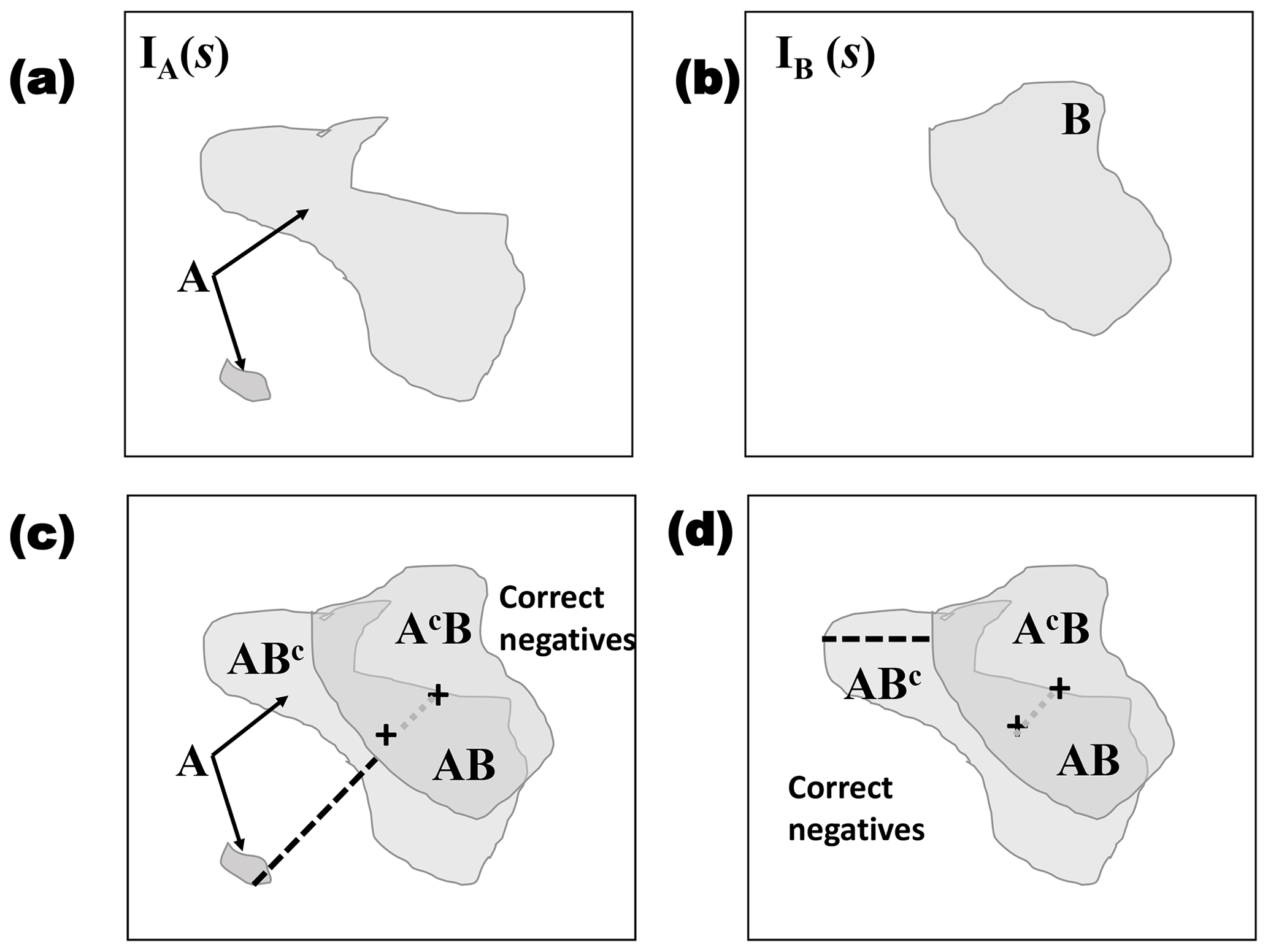
Figure 1 Illustration of two possible binary fields, namely (a) I_A and (b) I_B. Labels A and B indicate the areas (sets) of one-valued grid points, s, in each field, respectively. Set A contains two discontiguous areas (i.e., connected components), where B has one connected component. Panel (c) shows the same fields as in panels (a) and (b) overlaid on top of each other, along with a black dashed line indicating the Hausdorff distance and a gray dotted line indicating the centroid distance (+ signs show the centroid for each field). Here, AB indicates the area where A and B overlap (i.e., $I_A\left(\mathbf{s}\right)=I_B\left(\mathbf{s}\right)=\mathrm{1}$), AB^c where I_A(s)=1 and I_B(s)=0 (the superscript c stands for the set complement), and A^cB where I_A(s)=0 and I_B(s)=1. White areas are correct negatives (i.e., where I_A and I_B are both zero valued). Panel (d) is the same as panel (c) but where the smaller connected component from A is removed.

To simplify the discussion, it is useful to introduce some notation, which is depicted in Fig. 1. The figure displays two binary fields, I_A(s) and I_B(s). The set of locations s, where I_A(s)=1, is labeled as A and similarly for B. Define AB to be the set of s∈𝒟, where $I_A\left(\mathbf{s}\right)=I_B\left(\mathbf{\text{s}}\right)=\mathrm{1}$, AB^c is the intersection of the sets A and the complement of set B, or where I_A(s)=1 and I_B(s)=0, A^cB where I_A(s)=0 and I_B(s)=1, and, finally, A^cB^c where $I_A\left(\mathbf{\text{s}}\right)=I_B\left(\mathbf{\text{s}}\right)=\mathrm{0}$ (correct negatives). Let n_A (n_B) denote the number of grid points, where I_A(s)=1 (I_B(s)=1), and let n_AB be the number of grid points where both I_A(s)=1 and I_B(s)=1 (i.e., the area of overlap between A and B). Finally, let N be the total number of grid points in 𝒟, i.e., the size of the domain.

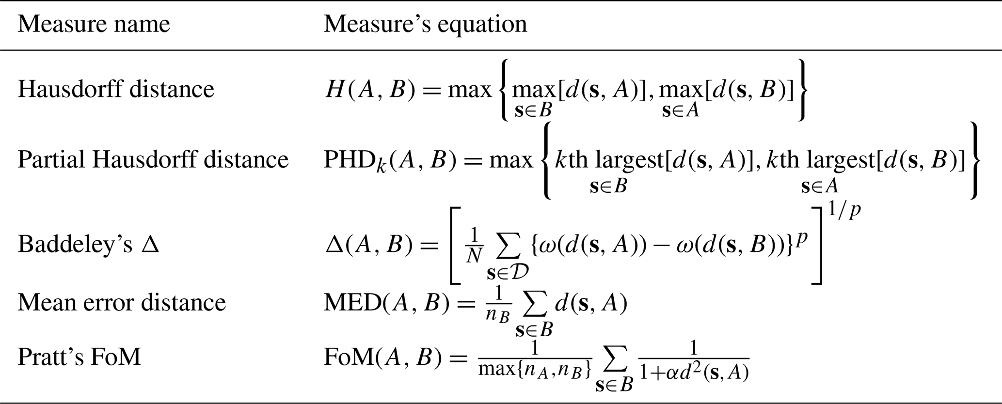
Table 1 gives the equations for the distance-based measures described subsequently.

Table 1 Equations for distance-based measures discussed here. Let $\mathbf{s}=(x,y)\in \mathcal{D}$ represent a grid point (coordinate) in the domain 𝒟, and let N be the size of the domain with $A,B\subset \mathcal{D}$ representing sets of grid points for which the corresponding value is one (in the binary field). Then let d(s,A) be the shortest distance from s to A and, similarly, for d(s,B). If a field is empty of one-valued grid points, define $d(\mathbf{s},A)=D$ for some large value D, such as N. Let n_A and n_B represent the number of grid points in the sets A and B, respectively. Furthermore, let I_A(s)=1, if s∈A, or zero otherwise, which is similar for I_B(s). ω is any continuous function on [0,∞] that is concave, and p is a user-chosen parameter. Finally, α in figure of merit (FoM) is a user-selectable parameter (see text).

One of the most well-known binary image measures is the Hausdorff distance metric (Baddeley, 1992a, b). This metric is very useful, generally, but has some drawbacks. For example, it has a high sensitivity to small changes in one or both fields. Figure 1 illustrates this metric for a comparison between I_A(s) and I_B(s), when A has two connected components (see Fig. 1 caption) and when the smaller connected component is removed. Although the two versions of A are very similar, H(A,B) is very different. On the other hand, this metric can be particularly useful in the forecast verification domain when the interest is in verifying small-scale high-intensity events that can be isolated after applying a high threshold specifically because of its high sensitivity to noise.

Several modifications to the Hausdorff method have been proposed, and perhaps the most well-known is the partial Hausdorff distance (PHD_k), which replaces the innermost maxima with the kth largest order statistic, mean error distance (MED), and Baddeley's Δ metric (Peli and Malah, 1982; Baddeley, 1992a, b). One summary measure, proposed by Venugopal et al. (2005), which was specifically designed for spatial forecast verification, utilizes the PHD_k but also incorporates an intensity component, and is known as the forecast quality index (FQI). Because it involves intensity and location in its evaluation of forecast performance, it is omitted from Table 1 and is instead given here by the following:

$$\begin{array}{}\text{(1)}& {\displaystyle }{\displaystyle }\text{FQI}(A,B)={\displaystyle \frac{{\text{PHD}}_k(A,B)}{\overline{\mathit{\psi }}}}/{\displaystyle \frac{\mathrm{2}{\mathit{\mu }}_A{\mathit{\mu }}_B}{{\mathit{\mu }}_A^{\mathrm{2}}+{\mathit{\mu }}_B^{\mathrm{2}}}}\cdot {\displaystyle \frac{\mathrm{2}{\mathit{\sigma }}_A{\mathit{\sigma }}_B}{{\mathit{\sigma }}_A^{\mathrm{2}}+{\mathit{\sigma }}_B^{\mathrm{2}}}},\end{array}$$

where $\overline{\mathit{\psi }}$ is the average of PHD_k(A,C_i) over $i=\mathrm{1},\mathrm{\dots },m$ surrogate fields, C_i (randomly generated fields with the same probability density and spatial correlation structure as A) and μ_A (μ_B) are the mean intensities over nonzero grid points from the original fields from which A and B are derived, and σ_A (σ_B) are the analogous standard deviations. As applied to a verification set, the surrogate fields are made with reference to the observation field so, using the notation from Eq. (1), the observed/analysis field is always A. The range of values FQI takes is [0,∞), with zero representing a perfect match and increasing values implying decreasing forecast quality.

One alternative summary measure to compare two sets A and B is known as Pratt's figure of merit (FoM; Peli and Malah, 1982; Baddeley, 1992a, b; Pratt, 2007, Eq. 15.5-1). FoM has one user-chosen parameter, α, which is a scaling constant that is typically set to one-ninth, corresponding to when $d(\cdot ,\cdot )$ is normalized so that the smallest nonzero distance between neighboring s is one, and $\mathrm{0}<\text{FoM}(A,B)\le \mathrm{1}$ with $\text{FoM}(A,B)=\mathrm{1}$ only if A=B. Like MED, FoM is not symmetric so that, generally, $\text{FoM}(A,B)\ne \text{FoM}(B,A)$. Figure 2 shows an example similar to one found by Peli and Malah (1982, and also shown in Baddeley, 1992b) that demonstrates how FoM is not sensitive to the pattern of displacement errors. In the example, the set A overlaps with B₂ but not B₁, although it is more similar in shape to B₁. Nevertheless, $\text{FoM}(A,B_{\mathrm{1}})\approx \text{FoM}(A,B_{\mathrm{2}})$ and $\text{FoM}(B_{\mathrm{1}},A)=\text{FoM}(B_{\mathrm{2}},A)$.

Figure 2 Similar to an example from Peli and Malah (1982). Suppose A represents the truth, and B₁ and B₂ are competing predictions for A. $G_{\mathit{\beta }}(A,B)=G_{\mathit{\beta }}(B,A)$ and $H_{\mathit{\eta }}(A,B)=H_{\mathit{\eta }}(B,A)$, but FoM does not share this symmetry property. Note that, when using $\mathit{\alpha }=\mathrm{1}/\mathrm{9}$, $\text{FoM}(B_{\mathrm{1}},A)=\text{FoM}(B_{\mathrm{2}},A)\approx \mathrm{0.5}$ and $\text{FoM}(A,B_{\mathrm{1}})\approx \text{FoM}(A,B_{\mathrm{2}})\approx \mathrm{0.9}$, indicating an insensitivity to shape. G_β, using $\mathit{\beta }=\mathrm{648}={\mathrm{6}}^{\mathrm{4}}/\mathrm{2}=N^{\mathrm{2}}/\mathrm{2}$, yields different values when comparing A with B₁ as opposed to A with B₂. Therefore, B₂ is favored because of the amount of overlap with A, whereas B₁ does not overlap with A at all. Nevertheless, G_β indicates a poor match for both B₁ and B₂ when compared with A at this level of β.

The same properties pointed out above also apply to MED (Baddeley, 1992b), except that MED is not bounded above by one. Additionally, MED is relatively sensitive to background noise, which is usually not desired unless the background noise is important (see an example in Gilleland, 2017, where the noise could be a severe storm).

Distance maps are useful for both describing and computing most of the distance-based methods. A distance map, $d(\cdot ,A)$, gives d(s,A) for every s∈𝒟 and can be calculated efficiently because of various distance transform algorithms (see Meijster et al., 2000; Brunet and Sills, 2017). Most, if not all, distance-based methods fail when one or both of the fields is empty (Gilleland et al., 2020). Some invoke a special rule so that they will be defined, but then their values tend to differ considerably if I_A(s₀)=1 at a single grid point s₀. For example, $d(\mathbf{s},A)=\mathrm{\infty }$ when A is empty, or in practice, $d(\mathbf{s},A)=D$, where D is some large number such as N. If, instead, I_A(s₀)=1 at a single point s₀ and I(s)=0 at all other points s≠s₀, then $d(\cdot ,A)$ will be much smaller than D at many locations, typically resulting in drastically different summary measure values even though the two fields are practically identical. Moreover, these measures may differ greatly, depending on where s₀ is located within 𝒟.

Some of the measures, such as MED, are susceptible to hedging because they are not very sensitive to frequency bias (Gilleland, 2017). Finally, most of these summary measures have zero as the value for a perfect match (e.g., if a field is compared against itself) but can be less straightforward to interpret in terms of what constitutes a poor forecast.

This paper presents the following two new measures: one that is free of any user-chosen parameters and another with a single user-chosen parameter that falls on a scale from zero to one, where one corresponds to a perfect match and zero to the user's idea of poor. The metrics incorporate not just the spatial alignment errors but also the frequency bias. Two additional summary measures are proposed that are based on the second location-only one but also incorporate a measure of intensity error that allows for the forecast to not be a perfect match without resorting to any computationally intensive or difficult-to-implement algorithms.

The new measures are computationally efficient, are not affected if the domain size is increased, cannot be hedged by increasing or decreasing the forecast frequency, and provide a single, easy-to-interpret summary of forecast performance that accounts for the amount of overlap between the forecast and observation and a graduated measure of the severity of any lack of overlap. Moreover, unlike all other distance-based summary measures, both of the new proposed metrics handle pathological cases naturally (see Sect. 4.1).

The equitable threat score (ETS) is also applied for some of the cases as a baseline comparison. The ETS is a hit-heavy traditional verification measure, so it does not account for the issues associated with high-resolution forecasts. Using the nomenclature of Fig. 1, ETS is defined by $(n_{AB}-r)/(n_{AB}+n_{A{B}^{\mathrm{c}}}+n_{A^{\mathrm{c}}B}-r)$, where $r=(n_{AB}+n_{A{B}^{\mathrm{c}}})(n_{AB}+n_{A^{\mathrm{c}}B})/N)$. ETS can be thought of as a strict, or even automaton, measure because it requires the overlap n_AB to be very high in order to pass muster.

1.2 The intensity conundrum

Because the main issue with traditional grid-point-to-grid-point verification is largely centered on the over-accumulation of errors in the face of spatial displacement errors, the most natural approach is to deform one or both of the forecast and observation fields so that they align better in space. Examples of this approach in the literature include a pyramidal matching algorithm (Keil and Craig, 2007, 2009), based on an approach that had been developed for the detection and tracking of cloud features in satellite imagery (Zinner et al., 2008), optical flow (Marzban and Sandgathe, 2010), and image warping (Gilleland et al., 2010; Gilleland, 2013). A feature-based method such as MODE can also be considered as a deformation approach in that individual features may be matched together and assumed to be aligned. In the case of MODE, the distributional intensity information is performed on these individual matched feature comparisons, so if it accumulated over features, then the result would be analogous to a deformation type of method. Beyond these approaches, only distributional information about intensities can be obtained.

Of the deformation methods proposed, the image-warping procedure is the only one that has an elegant statistical model that allows for a natural method to ascribe uncertainty information. Deformations that yield optimal, or near-optimal, spatial alignments are not unique, however. Moreover, while non-sensible and non-physical deformations can be penalized in the optimization procedure, there is no guarantee that they will not result; for example, it is possible for the entire field to be compressed into a ball or pushed out of the domain. The biggest challenge, however, may be simply in determining how best to weight the amount of deformation required versus the resulting error intensities.

The vast majority of spatial verification methods proposed are applied on binary fields usually obtained by setting all values below the threshold to zero and those above to one. Examples include the intensity-scale approach (Casati et al., 2004) and MODE, which also includes a distributional component for the intensities and all of the distance-based approaches discussed in Sect. 1.1. In this work, a distributional measure of intensity performance is proffered that is combined with the new spatial alignment measure, G_β, described in Sect. 2. It is not a fully satisfactory measure, as will be seen, but it can be useful in some situations. Moreover, it represents a best-case deformation summary – if there were no considerations about how much deformation should be allowed.

2 The new measures

Having a summary measure that penalizes misses and false alarms in a consistent and sensible manner is desired. It should be sensitive to small changes in one or both fields but not overly so. If the (binary) forecast contains a set, A, of one-valued grid points and the observation set, B, then the value of the measure should not change if A and B are found in a different part of the domain, or are rotated, as long as they are the same relative to each other (see the first few circle cases from Gilleland et al., 2020 that are also analyzed subsequently here).

Therefore, the new measures involve a term, denoted by y₁, that measures the lack of overlap by way of the size of the symmetric difference. Another term, y₂, provides a measure of the average distance of A to B and B to A, weighting each by the size of the two sets in order to mitigate the impact of this term in the event that a set is small.

Let y=y₁y₂ where $y_{\mathrm{1}}=n_{A\mathrm{△}B}=n_{A{B}^{\mathrm{c}}\cup A^{\mathrm{c}}B}=n_A+n_B-\mathrm{2}{n}_{AB}$ and $y_{\mathrm{2}}={\sum }_{\mathbf{s}\in B}d(\mathbf{s},A)+{\sum }_{\mathbf{s}\in A}d(\mathbf{s},B)=\text{MED}(A,B)\cdot n_B+\text{MED}(B,A)\cdot n_A$, with MED as in Table 1. Both new measures are functions of the product y₁y₂. This product multiplies an area and a distance with units of grid points squared and grid points, respectively. The first measure, therefore, is a cubed root of this product so that the resulting value has the same units as most of the other distance-based measures (i.e., grid points) described in Sect. 1.1. The second is a unitless quantity that is rescaled so that it falls between zero and one, with zero being a bad score and one being a perfect score. The new performance measures applied to compare two binary fields, I_A(s) and I_B(s) (as described in Fig. 1), are given by the following:

$$\begin{array}{}\text{(2)}& {\displaystyle }{\displaystyle }G(A,B)=y^{\mathrm{1}/\mathrm{3}},\end{array}$$

and

$$\begin{array}{}\text{(3)}& {\displaystyle }{\displaystyle }{G}_{\mathit{\beta }}(A,B)=max\left\{\mathrm{1}-{\displaystyle \frac{y}{\mathit{\beta }}},\mathrm{0}\right\},\end{array}$$

where β>0 is a user-chosen parameter. Equation (3) represents a fuzzy-logic scaling of y that falls between zero (exceptionally poor forecast) and one (perfect forecast) in the same vein as an interest value in the MODE approach (Davis et al., 2006a, b, 2009). Indeed, G_β applied to individual features would be a good alternative to the centroid distance that is often used as part of MODE.

The term y₁, which, again, is a penalty for lack of overlap between A and B, has a maximum possible value of N, which happens when $n_A+n_B=N$ and n_AB=0. In the case of a perfect match (i.e., A=B), y₁=0. It is the size of the symmetric difference, A△B, between the two sets, and its units, therefore, are numbers of grid points squared.

MED(A,B) is a measure of average distance from B to A in terms of the distance $d(\cdot ,\cdot )$ described previously. In general, $\text{MED}(A,B)\ne \text{MED}(B,A)$. Because MED is not sensitive to the occurrence rate, each MED in y₂ is multiplied by its respective size, n_A or n_B. This compensation ensures that a large MED will not overly dominate the resulting measure when sets A or B are small. The units, here, for y₂ are grid points so that the units for the product y₁⋅y₂ are numbers of grid points cubed. Therefore, G from Eq. (2) has numbers of grid points as its units.

For a perfect match, $\text{MED}(A,B)=\text{MED}(B,A)=\mathrm{0}$ and, subsequently, y₂=0. The maximum value for MED is D (where D is a large value as described in Sect. 1.1), which would occur when n_A=N and n_B=0 for MED(B,A) or, similarly, when n_A=0 and n_B=N for MED(A,B). Because MED(A,B) is undefined if n_B=0, the term $\text{MED}(A,B)\cdot n_B$ is defined to be zero in this situation and, similarly, for $\text{MED}(B,A)\cdot n_A$ when n_A=0. Tempering the MED in this way ensures that small amounts of noise will not overly affect the results, unlike untempered MED. Gilleland (2017) argued that MED's sensitivity to noise could be useful when smaller-scale spatial events are important (e.g., storm activity), and it should be noted that G_β can be useful in this capacity through careful choice of the β argument as described below. The Hausdorff distance, as mentioned previously, is particularly well suited to such a verification.

The product y=y₁y₂ provides a measure of the size of the area given by AB^c and A^cB magnified by a measure of the distance between A and B. The function in Eq. (3) decreases linearly in y from one (perfect match) to zero (very poor forecast). The maximum possible value of $y_{\mathrm{1}}{y}_{\mathrm{2}}=N^{\mathrm{2}}\cdot D$, which provides some motivation for choosing β and is to be chosen with N and the base rate in mind. Experimentation has found that $\mathit{\beta }=N^{\mathrm{2}}/\mathrm{2}$ is a sensible choice when the base rate is large but small relative to N (see Fig. 2 and the cases in Gilleland et al., 2020), but if penalizing location errors more greatly is desired, then smaller values for β can be used. For example, Fig. 3a, c, and e demonstrate both G_β, with three different choices of β, and FoM, with three different choices of α, applied to a comparison between two identical circles, where one circle is translated horizontally by increasing amounts. If β is small ($\mathit{\beta }=N\sqrt{N}$), then G_β decreases rapidly with increasing translation errors and equals zero once it is separated by 20 grid squares, or the point at which there is no longer an overlap between the two circles. When $\mathit{\beta }={\mathrm{200}}^{\mathrm{4}}/\mathrm{2}$ or 200⁴, G_β decreases more slowly, giving more credit to forecasts with larger displacement errors. When β=200⁶, G_β decreases but remains very close to one for all circles. The FoM applied with three different values of α demonstrates that this scaling constant does not affect the result very much, and the measure decreases rapidly with increasing translation errors.

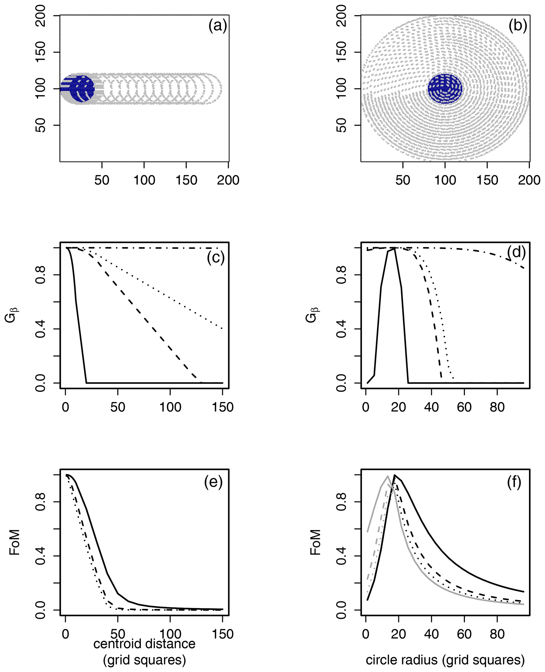
Figure 3 G_β (c, d) and FoM (e, f) applied to pairs (a) consisting of the leftmost blue solid circle and identical, horizontally translated circles (outlined for clarity) and (b) the blue solid circle with circles centered on the same location but with varying radii. Each set of comparisons is on a 200×200 domain. The blue solid circles have radii of 20 grid points. G_β lines are $\mathit{\beta }={\mathrm{200}}^{\mathrm{3}}=N\sqrt{N}$ (solid), $\mathit{\beta }={\mathrm{200}}^{\mathrm{4}}/\mathrm{2}=N^{\mathrm{2}}/\mathrm{2}$ (dashed), $\mathit{\beta }={\mathrm{200}}^{\mathrm{4}}=N^{\mathrm{2}}$ (dotted), and $\mathit{\beta }={\mathrm{200}}^{\mathrm{6}}=N^{\mathrm{3}}$ (dot dashed). FoM lines are $\mathit{\alpha }=\mathrm{1}/\mathrm{100}$ (solid), $\mathit{\alpha }=\mathrm{1}/\mathrm{9}$ (dashed), and $\mathit{\alpha }=\mathrm{1}/\mathrm{2}$ (dotted). $\text{FoM}(A,B)\ne \text{FoM}(B,A)$, generally, but is symmetric for the left column comparisons. Black lines for FoM in panel (f) indicate FoM(A,B), and gray lines indicate FoM(B,A).

Figure 3b, d, and f show a similar analysis for G_β and FoM but for different types of bias. For the highest values of β applied, the smaller radii are not small enough for G_β to drop much below the perfect value, though they do drop. In this case, the lowest choice of β perhaps supplies the optimal behavior. FoM behaves well, and in this case, the asymmetry of the measure is apparent as the gray and black lines reflect a similar pattern but do not give the same result for each comparison.

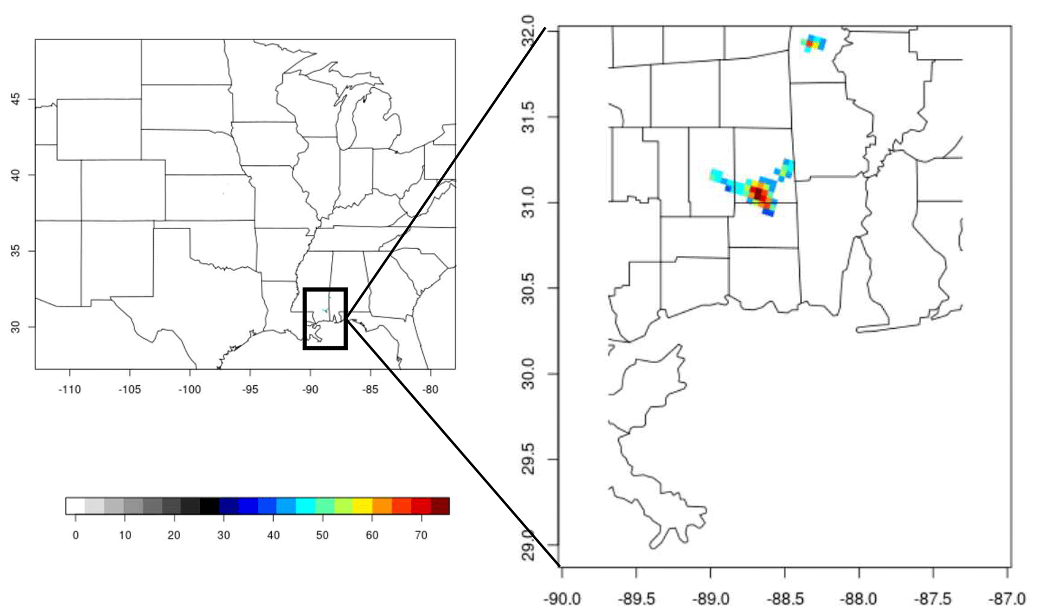
Figure 4 An example of 24 h accumulated precipitation forecast displaying only those values that exceed 40 mm h⁻¹. The forecast is the Inter-Comparison Project (ICP) wrf4ncar case for 1 June 2005 (Ahijevych et al., 2009).

Because G and G_β are designed, in part, to seamlessly handle the pathological cases, they will typically yield good scores at high thresholds because the areas that exceed those thresholds are typically very small in both fields. If such high intensities over such small areas are important (e.g., severe thunderstorms), then a lower choice of β can be used. Figure 4, for example, shows a precipitation forecast only for values exceeding 40 mm h⁻¹. The observation is not shown but, to the naked eye, appears identical (i.e., empty). However, the observation has no precipitation exceeding 40 mm h⁻¹ anywhere near the enlarged region of southern Louisiana and Alabama displayed, where, clearly, the forecast has rather intense false alarms. Over the entire domain, the observation field has three connected components with areas of 18, 132, and 11 grid points, whereas the forecast has only two such areas of five and 37 grid points (both shown in Fig. 4). That is, there are also areas with intense precipitation that were missed by the forecast. Taking, as an exceptionally large area for this activity, about 200 grid squares and supposing that an average distance of 20 grid squares (≈80 km) is too large of a translation error, then $\mathit{\beta }=\mathrm{200}\cdot \mathrm{20}=\mathrm{4000}$ is an appropriate choice for β. Indeed, G_β=0 for this choice with this verification set and a threshold of 40 mm h⁻¹.

The flip side of choosing β is that a particular user might only be interested in egregious errors so that a higher choice of β will be appropriate as the score will be more forgiving. In general, when reporting results for G_β, it is important to specify the choice of β and the reasoning behind it. When possible, physical reasoning should be employed.

A modification is presented for incorporating intensity information into G_β, denoted G_β,IL, where IL stands for intensity and location. G_β can be thought of as a type of summary of the amount of deformation that would be required if one could completely transmogrify the field so that all intensity values were matched with the nearest such value in the other field. Therefore, any type of distributional measure of the similarities in intensities completes the picture for this paradigm. Of course, a calibrated forecast should already match the distribution of the observed field in this way so that the additional measure may be less important than the alignment errors. It is given by the following:

$$\begin{array}{}\text{(4)}& {\displaystyle }{\displaystyle }{G}_{\mathit{\beta },\text{IL}}(A,B)=\mathit{\omega }\cdot G_{\mathit{\beta }}(A,B)+(\mathrm{1}-\mathit{\omega })\cdot \mathit{\theta }(A,B),\end{array}$$

where θ(A,B) is $max\mathit{\left\{}\mathit{\rho }\right(A,B),\mathrm{0}\mathit{\}}$, with ρ the linear correlation coefficient between sorted values of the intensities within the set A and those in the set B, and ω is a user-chosen weight dictating the importance of spatial alignment errors versus intensity errors, which are defined distributionally.

If the distribution of values in A is the same as that in B, then the relationship between their sorted values should be a straight line, and correlation measures the strength of this linear relationship. Because the sorted values are both monotonically increasing, θ(A,B) will generally be high. Nevertheless, when the distributions are different, their value will decrease. In general, ω should be higher than one-half in order to weigh the more important spatial alignment errors more heavily.

Equation (4) assesses intensity performance distributionally through the sorted intensity values within the sets A and B. If n_A<n_B or n_B<n_A, then the larger set of sorted values is linearly interpolated to have the same size as the smaller set. A difficulty arises when n_A=0 or n_B=0. For θ(A,B), it is unclear what do for such cases. If $n_A=n_B=\mathrm{0}$, then θ(A,B) could be taken to be one, and if the non-empty set is small, then it could be taken to be something near to one, but the solution to this problem will be application dependent and is not discussed further here.

The motivation for using the sorted values in θ is that y₁ measures lack of overlap, and y₂ provides a sense of the closeness of the lack of overlap, so θ can be thought of as the intensity error remaining if they could be realigned spatially so that they match up in an optimal way. In this way, it can be thought of as a quick and easy field deformation type of summary. Another interpretation, already mentioned, is that it is a distributional comparison of the nonzero-valued intensities analogous to those from a quantile–quantile (q–q) plot. In fact, a q–q plot of the values in the set A compared with those in B is a scatter plot of exactly the same sorted, and possibly interpolated to the same size, intensities.

3 Test cases

Several test cases are employed in order to demonstrate the behavior of G_β and G_β,IL. Comparisons of G_β are made with FoM and G_β,IL with FQI from Eq. (1) because these existing measures appear to be the most similar. The first set of test cases is applied to understand G_β and comes from the recently proposed set of comparisons by Gilleland et al. (2020),¹ namely the pathological, circle, ellipse, and noisy comparisons.

For G_β,IL, 3 h accumulated precipitation (in millimeters) from the core case of the Mesoscale Verification Inter-Comparison over complex Terrain project is used (MesoVICT; https://ral.ucar.edu/projects/icp/, last access: 11 February 2021; Dorninger et al., 2013, 2018). The precipitation case utilizes the Vienna Enhanced Resolution Analysis (VERA, Steinacker et al., 2000) as observation and the Canadian high-resolution model (CMH; Dorninger et al., 2013, 2018). The case is a subset of the minimum core case from the MesoVICT project and involves several valid times between 20 and 22 June 2007. Here, only 3 h of accumulated precipitation for the 12 h lead times is analyzed. Figures 5 to 7 show plots of these cases, along with diagnostic plots described in Sect. 5.

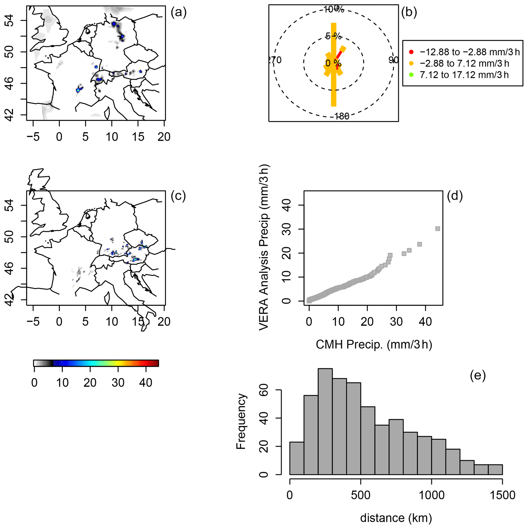
Figure 5 MesoVICT case 1 verification set, ending on 20 June 2007, at 18:00 coordinated universal time (UTC), for 3 h accumulated precipitation, given in millimeters (a, c). VERA analysis (a) and CMH with a 12 h lead time (b). Circle histogram (analogous to a wind rose diagram) showing the sorted model values, minus the sorted analysis values, and binned by the bearing from the analysis to the model (referenced from the north) of these sorted values (b). A q–q plot of VERA against CMH over all values (d). A histogram for the distances between the sorted values of the analysis and the model (e). See Sect. 5 for a detailed explanation of this figure.

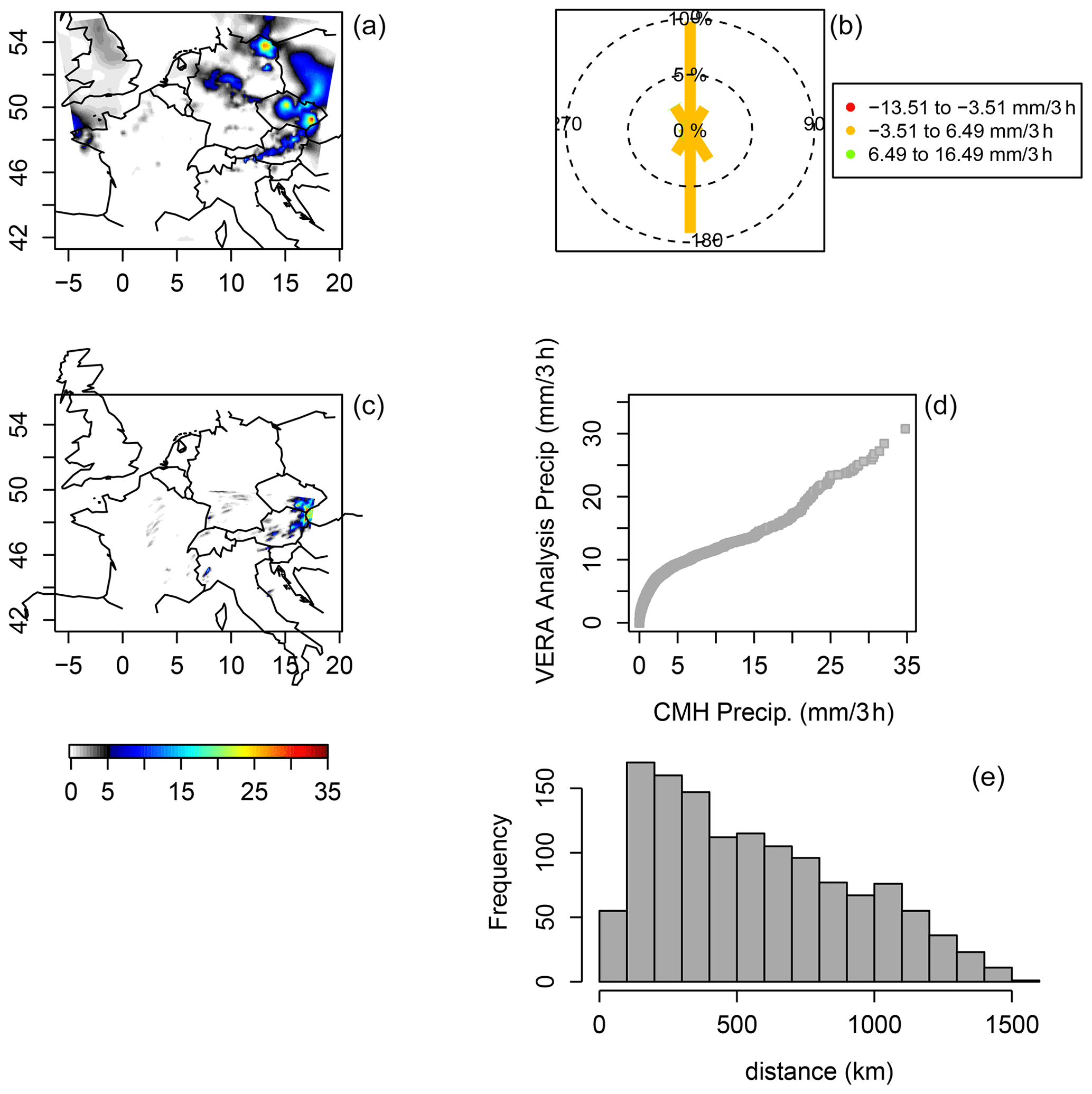
Figure 6 Same as Fig. 5 but ending on 21 June 2007.

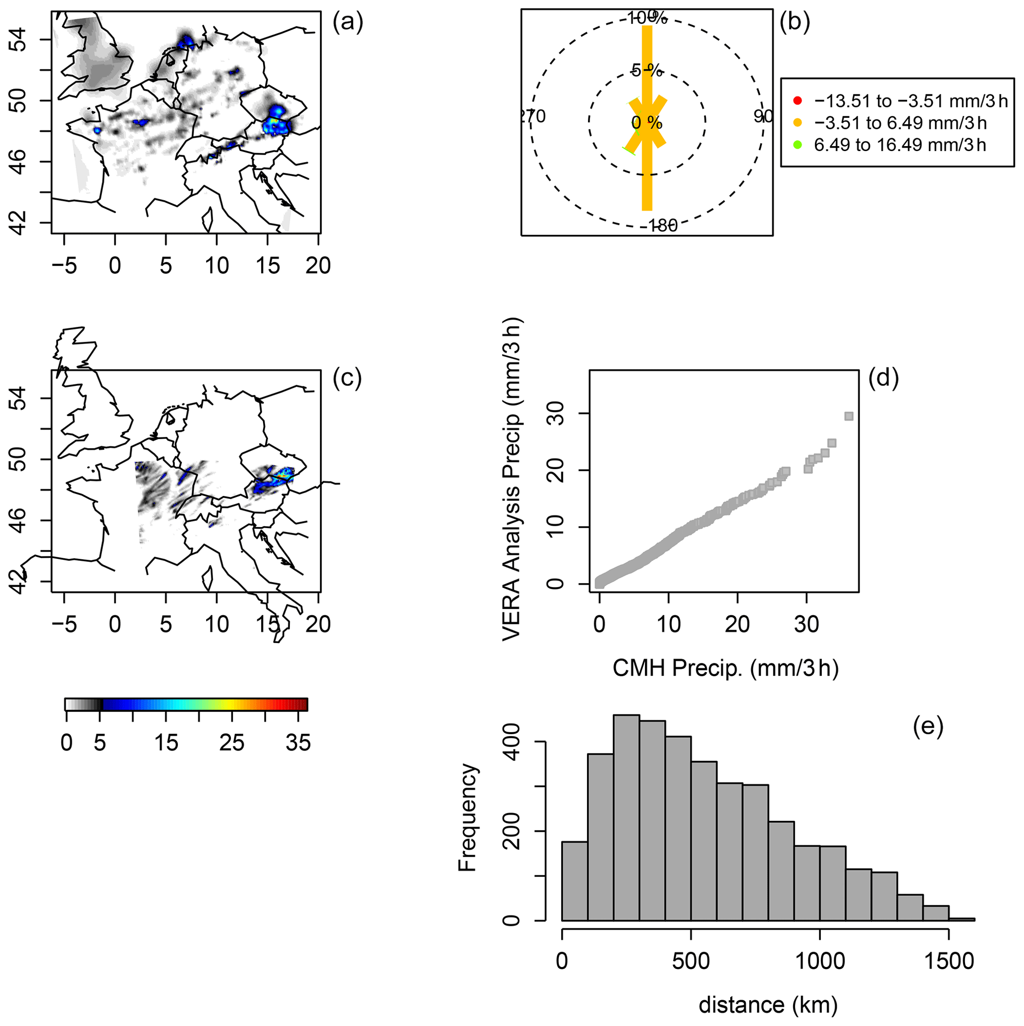
Figure 7 Same as Fig. 5 but ending on 22 June 2007.

Finally, in order to provide a more thorough test of G_β,IL, the 32 spatial forecast verification ICP real test cases are also analyzed. These contain two models, namely the Advanced Research Weather Research and Forecasting Model (ARW-WRF; Skamarock et al., 2005) and the nonhydrostatic mesoscale model (NMM). Stage II reanalysis is used as the observations. These cases were previously analyzed by Davis et al. (2009) for MODE, Gilleland et al. (2010) and Gilleland (2013) with image-warping and hypothesis-testing procedures, and Gilleland (2017) using MED. The forecasts were initialized at 00:00 UTC (early evening), with a 24 h lead time, and were part of the 2005 National Severe Storms Laboratory and Storm Prediction Center Spring Program (Baldwin and Elmore, 2005). See Kain et al. (2008) and Ahijevych et al. (2009) for more information on these cases.

The development of spatial verification measures largely grew out of the specific application of verifying quantitative precipitation forecasts, which is the reason why the ICP and MesoVICT cases are focused on these types of fields. Nevertheless, G and G_β, and most of the spatial verification methods, can be applied to other types of variables such as wind speed. In the case of the distance-based measures, including G and G_β, as long as the variable field can be sensibly converted into a binary field, then the measures can be applied.

4 Application to the new geometric cases from MesoVICT

Gilleland et al. (2020) applied the Hausdorff distance, Baddeley's Δ, and MED to the test cases developed therein, so those results can be compared with the results for G and G_β in this section. Because FoM has not been considered on these cases previously, and because it is the most similar to G_β, it will also be evaluated and compared here. For brevity, G is only applied to the circle cases as results are generally consistent with G_β, which means essentially comparing the functions $f_{\mathrm{1}}\left(x\right)=x^{\mathrm{1}/\mathrm{3}}$ with $f_{\mathrm{2}}\left(x\right)=\mathrm{1}-x/\mathit{\beta }$ for $x/\mathit{\beta }\ge \mathrm{0}$.

4.1 Pathological cases

The pathological comparisons represent challenging, but often encountered, situations where fields are empty, full, or contain only some small amounts of noise. Each individual field is on a 200×200 domain, as described in Table 2, and is labeled P1 to P7. A total of two comparisons also involve a circle of radius 20 centered at (100,100) and labeled C1.

Table 2 Description (top) of the pathological fields from Gilleland et al. (2020). Each field is on a 200×200 domain, 𝒟, with $\mathbf{s}=(x,y)$ giving the x and y coordinates such that (1,1) is the lower left corner. Results (bottom) for G_β for comparisons of the pathological cases. The value ≈1 indicates that G_β<1 but G_β=1.00 after rounding to two (or even more) decimal places.

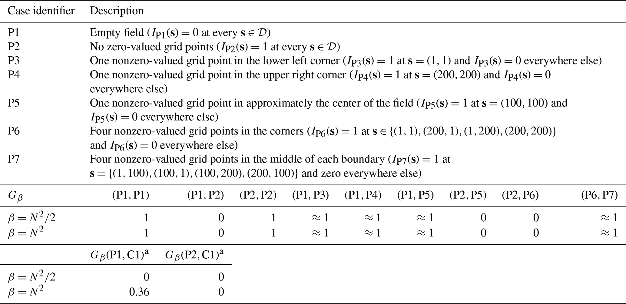
^a C1 is a circle of radius 20 centered at the point (100,100).

All of the distance-based measures tested by Gilleland et al. (2020) were either undefined or gave erratic results for the pathological comparisons. Table 2 demonstrates that G_β, using $\mathit{\beta }=N^{\mathrm{2}}/\mathrm{2}=(\mathrm{200}\cdot \mathrm{200}{)}^{\mathrm{2}}/\mathrm{2}$, behaves naturally even for the most difficult of these tests. The comparisons of P1 against P1 (henceforth denoted by P1P1 and similarly for other comparison labeling) and P2P2 yield G_β values that are identically one, which is desired as they are perfect matches. When one or a few one-valued grid points are added to the empty field (i.e., cases P3, P4, P5, P6, and P7), the comparisons P1P3, P1P4, P1P5, and P6P7 in the figure yield G_β values that are very close to, but slightly less than, one. Because these fields are largely identical outside of this small amount of noise, a G_β near one is the result that is wanted.

On the other hand, the comparison between P1 and P2, which represents a worst-case scenario of an empty field (I_P1(s)=0 at every s∈𝒟) compared to the full field, P2 (I_P2(s)=1 at every s∈𝒟) yields $G_{\mathit{\beta }}(\text{P1},\text{P2})=\mathrm{0}$, as desired. The comparisons P2P5 and P2P6 are comparisons that are nearly identical to the comparison P1C1, except that, again, P5 and P6 have four nonzero-valued grid points. G_β=0 for these comparisons, agreeing with the subjective judgment. It is also zero for the comparison P2C1, which compares the full field against a field with a relatively small circle of one-valued grid points.

Finally, G_β(P1,C1) has a relatively higher value than for G_β(P2,C1), if $\mathit{\beta }=(\mathrm{200}\cdot \mathrm{200}{)}^{\mathrm{2}}$ (right), and for $\mathit{\beta }=(\mathrm{200}\cdot \mathrm{200}{)}^{\mathrm{2}}/\mathrm{2}$ (left), its value is zero (the same as for P2C1). For the higher β, the large amount of correct negatives allows for a better score for P1C1 than P2C1. The zero-value of G_β for P2C1 is, quite correctly, suggestive of a poor match as desired, regardless of whether $\mathit{\beta }=(\mathrm{200}\cdot \mathrm{200}{)}^{\mathrm{2}}$ or $(\mathrm{200}\cdot \mathrm{200}{)}^{\mathrm{2}}/\mathrm{2}$.

Pratt's FoM is not defined whenever it is calculated from the empty field P1 because there is no non-empty set of one-valued grid points from which to calculate the distance map (including FoM(P1,P1), FoM(P1,P2), etc.). If using the rule that $d(\cdot ,A)=D$ for large D when A is empty, then FoM will be near zero for any comparison from P1. FoM for each of the remaining comparisons is very close to zero, indicating that each pair of fields is a poor match, which is not consistent with a subjective evaluation. That is, the empty field creates a situation where FoM is either not defined, or it suggests a bad match regardless of whether the match is very good or very bad.

4.2 Circle comparisons

Figure 8 shows results for G from Eq. (2) applied to the circle comparisons, and Fig. 9 shows the results for G_β and FoM applied to the circle and ellipse comparisons proposed by Gilleland et al. (2020, Figs. 5 and 6). Small dotted vertical lines separate similar comparisons as a visual aid. The first five circle comparisons demonstrate that neither G nor G_β is sensitive to the positioning of the one-valued grid points within the domain. That is, they give the same value for the first three comparisons, which are identical comparisons, apart from their positions within 𝒟, which is similar for the next two comparisons (C1C4 and C3C4). This property is desirable but is not achieved by all summary measures, including Δ. The first three comparisons represent identical circles that are translated so that they touch at one point but do not overlap. G_β penalizes them for the lack of overlap but otherwise gives these cases a relatively high mark. G is less readily interpreted, but its relative value for the comparisons is consistent with the other distance-based measures applied in Gilleland et al. (2020). C1C4 and C3C4 are also identical circles but have been translated further apart, and this additional translation error is penalized more than with the first three cases. FoM, while generally not symmetric, is symmetric for the first 11 comparisons and for C1C10, C6C12, and C13C14. FoM penalizes the first five comparisons considerably, yielding values very near to zero.

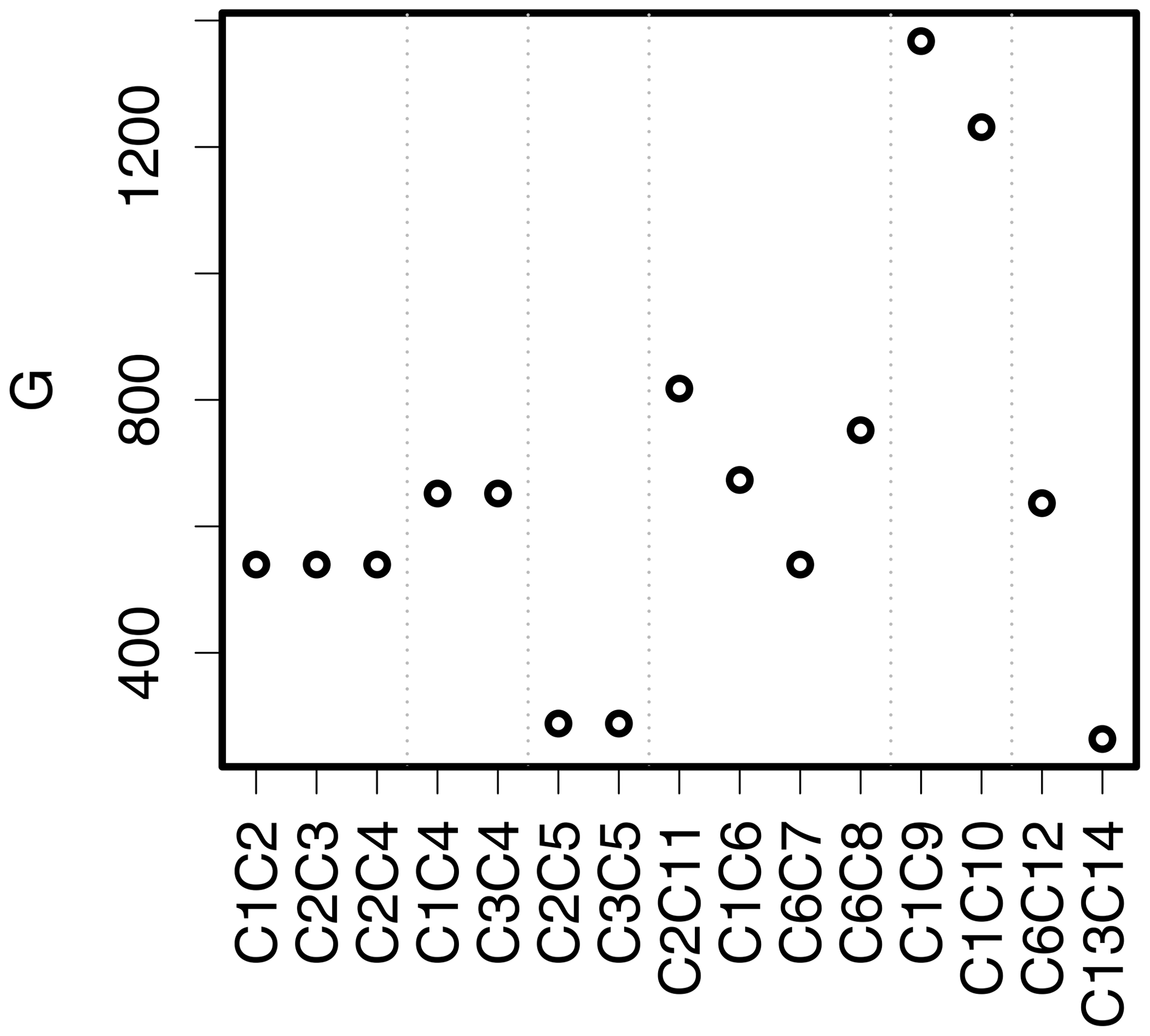
Figure 8 Results for G from Eq. (2) applied to the circle comparisons from Gilleland et al. (2020). Smaller values are better, and zero signifies a perfect match. Dotted vertical lines separate similar comparisons as a visual aid.

Figure 9 G_β and FoM results for the geometric comparisons from Gilleland et al. (2020), which are on a 200×200 gridded domain. At the top are the circle comparisons, and at the bottom are the ellipse comparisons. Black solid circles indicate G_β values (using $\mathit{\beta }={\mathrm{200}}^{\mathrm{4}}/\mathrm{2}=N^{\mathrm{2}}/\mathrm{2}$), gray circles are FoM(A,B), and gray + signs are FoM(B,A), where A represents the first case in the label, e.g., C1 from C1C2 and B the second; $\mathit{\alpha }=\mathrm{1}/\mathrm{9}$. Dotted vertical lines separate similar comparisons as a visual aid.

C2C5 and C3C5 are similar comparisons as for C1C2, for example, except that these circles overlap as they are not translated as far. Their G_β values are subsequently very near to one, but their FoM values are relatively low at about 0.6. G≈288.86 for both of these comparisons, which puts them in a tie for second in terms of ranking the quality of the matches across the comparisons (C13C14 is better, according to G, with a value of about 263.99).

C2C11 is a comparison in which C11 is the union of the three circles C1, C3, and C4 against C2 and was originally introduced in Gilleland (2017) in testing the MED. It was found that MED(C2,C11) gave the same value as it gave for the C1C2, C2C3, and C2C4 comparisons, but MED(C11,C2) was much smaller. C1C6 is a similar comparison, but with only two additional circles, and results are similar for this comparison. G and G_β are symmetric, so there is no difference between, for example, G_β(C2,C11) and G_β(C11,C2), and both penalize this comparison because of the lack of overlap and the additional circles. FoM does not distinguish this comparison at all from the C1C2, C2C3, and C2C4 comparisons, again indicating its inability to distinguish shape errors.

C7 and C8 have the same upper circle as C6, but the lower circle is offset, with C7 more so than C6. $G(\text{C6},\text{C7})=G(\text{C1},\text{C2})$ and $G_{\mathit{\beta }}(\text{C6},\text{C7})=G_{\mathit{\beta }}(\text{C1},\text{C2})$ because, despite having a perfect match with the upper circle, the error with the lower circle in C6C7 is identical to the error between C1 and C2. FoM, on the other hand, is much higher for C6C7 than C1C2. Thus, FoM rewards more for having some more parts correct than G_β.

C9 is a circle with the same center as C1 (centroid distance is zero) but is much larger. $G_{\mathit{\beta }}(\text{C1},\text{C9})=\mathrm{0}$, using $\mathit{\beta }={\mathrm{200}}^{\mathrm{3}}/\mathrm{2}$, whereas FoM is very low but not identically zero. $G(\text{C1},\text{C9})\approx \mathrm{1367.67}$ is a high value and shows this case to be the worst of the circle comparisons. C1C10 is a similar comparison, but the larger circle is replaced with a ring so that C10 does not intersect with C1, and there is a gap between them. Again, the centroid distance is zero (perfect score), but both G_β and FoM are zero (worst score possible). $G(\text{C1},\text{C10})\approx \mathrm{1231.91}$ is also a high value, indicating a poor match, but is lower than for C1C10, which contrasts with Δ, which was found to have approximately the same value for these comparisons.

C6C12, similarly, has a centroid distance of zero this time because the two circles in C12 are translated equally but in opposite directions from the two circles in C6, and each circle in C12 overlaps with the two circles in C6. G_β is relatively high for this case, but lower than for the first three comparisons, penalizing for the additional area that is not overlapped. $G(\text{C6},\text{C12})\approx \mathrm{637.59}$ is again difficult to interpret in terms of good versus bad but suggests that, relative to the other comparisons, it is much better than the most egregious error comparisons.

Finally, G_β and FoM disagree completely about how good of a match there is between C13 and C14. Both sets of circles include much smaller circles than before, so G_β (with $\mathit{\beta }=N^{\mathrm{2}}/\mathrm{2}$) does not penalize the relatively small translation errors as much. On the other hand, FoM greatly penalizes them for this case, ignoring the circle sizes.

As discussed in Sect. 2, the FoM result for C13C14 (see Fig. 10a) might be the more desired result for this case if these relatively small circles represent an event such as severe weather rather than unimportant noise. In such a case, G_β can still be effective if the value of β is chosen with the physical interpretation in mind. For example, the base rate for C1 (i.e., $n_{\text{C1}}/N$) is a little larger than 0.03, whereas it is less than 0.01 for C13 and C14. The total size $n_{\text{C13}}=n_{\text{C14}}=\mathrm{362}$, and assuming each grid square represents, say, 4 km, then one might consider an error of 10 grid squares (≈40 km) to be too large. In fact, the largest circles in C13 and C14 have a radius of eight grid squares. Therefore, an upper bound for a very poor match for y from Eq. (3) might be considered to be about $\mathrm{350}\cdot \mathrm{10}=\mathrm{3500}$. Figure 10b shows G_β(C13,C14) for varying values of β. The left vertical line is through β=3500, and the right vertical line is through $\mathit{\beta }=N^{\mathrm{2}}/\mathrm{2}=\mathrm{20}\mathrm{000}$ that is used for the above results. In other words, if the small circles in the figure are important, then a smaller value of β should be used, and if they represent noise, then a higher value is in order. G_β=3500 correctly informs that these two cases are not close enough, whereas $G_{\mathit{\beta }=N^{\mathrm{2}}/\mathrm{2}}$ indicates a fairly good match.² G gives the lowest value for this comparison out of any of the other comparisons, indicating it is the best match. If the application needs these cases to be more heavily penalized, then G is not the ideal choice of measure, and the Hausdorff distance would be recommended.

4.3 Ellipse comparisons

The ellipse comparisons (Gilleland et al., 2020, Figs. 7 and 8) are shown in the lower panel of Fig. 9, and abstract the types of situations common over complex terrain. The vertical dotted lines again provide a visual aid to separate different types of errors represented in the comparisons, namely, (i) translation-only errors, followed by (ii) size-only errors, (iii) size and translation errors, (iv) rotation only errors, (v) rotation and translation errors, and (vi) rotation, translation, and size errors, and (vii) the final three comparisons involve a single ellipse compared against several small ellipses within a larger elliptical envelope and three ellipses compared against a larger blob that roughly follows the shape of these ellipses.

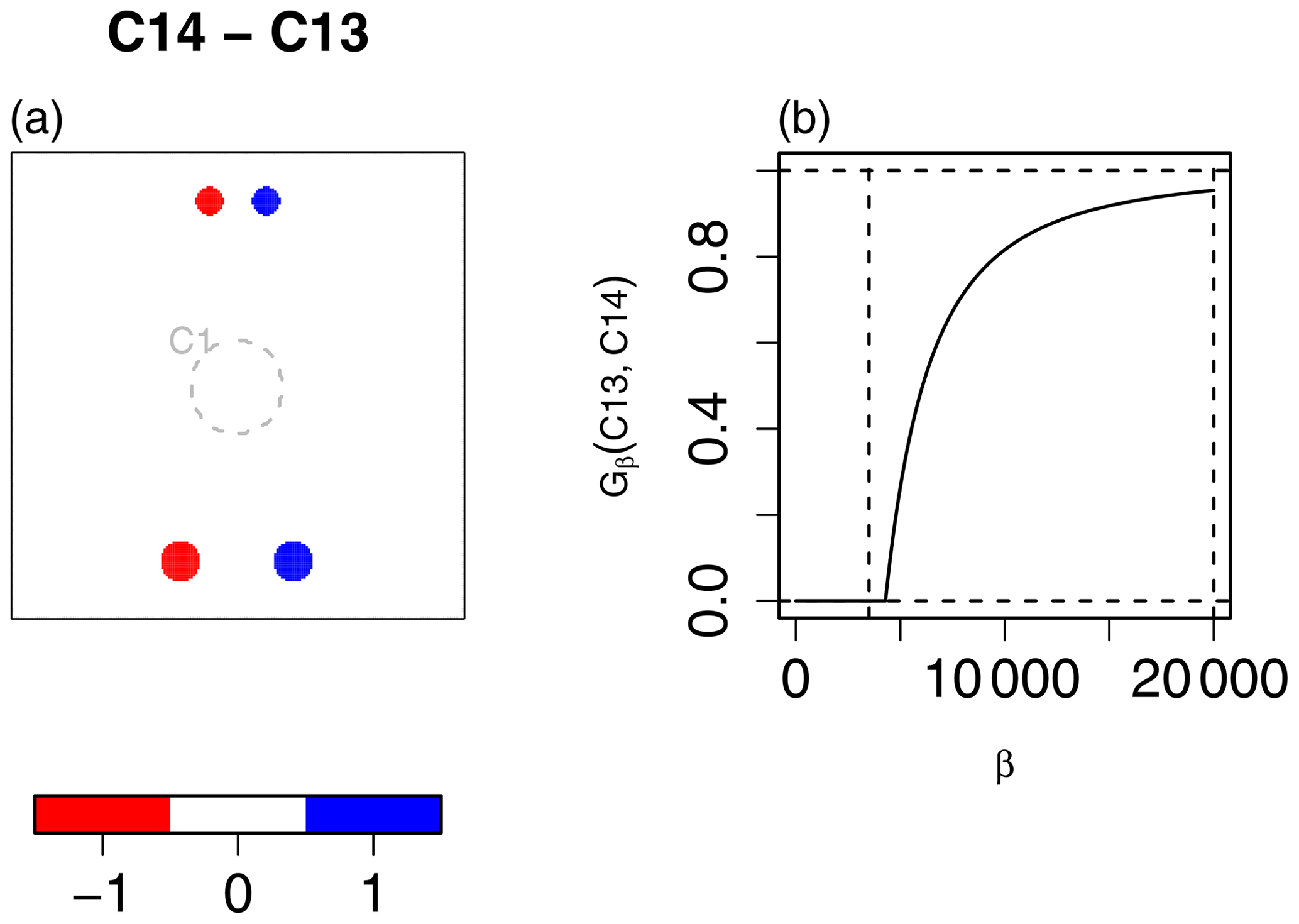
Figure 10 (a) The C13C14 comparison shown as the difference C14 − C13. The size of the one-valued set is small relative to the size of the domain. The base rate is less than 0.01 for both fields. The total size of these sets is 362. For comparison in terms of the spatial areas of the circles, the gray dashed circle in the center shows C1. (b) G_β(C13,C14) applied with a range of different β values. The left vertical line is through β=3500, and the right vertical line is through $\mathit{\beta }=N^{\mathrm{2}}/\mathrm{2}=\mathrm{20}\mathrm{000}$.

G_β and FoM disagree considerably on the quality of the match for the translation-only errors, where, in this case, G_β perhaps gives a value (around 0.8) that is more consistent with a subjective evaluation because the ellipses are identical – apart from a relatively small translation (no overlap). FoM, on the other hand, gives a value very close to zero. They also disagree on E7E11, which is a similar comparison, except that one of the ellipses is much smaller than the other. G_β again gives a high value (higher than for the first several comparisons), and FoM is again very low and even closer to zero in this particular comparison. Finally, they also disagree on E2E18 in the same way. This case again involves a translation error and essentially a size error. One might agree more with FoM that this match quality is poor, but if the small-scale detail is less important than the overall size and shape of the extent of, say, the type of convective activity in complex terrain for which this comparison was designed, then G_β provides a sensible result.

Otherwise, the two measures generally agree with each other in relative terms; that is, they rank the remaining comparisons similarly. G_β generally results in fairly high values for all of these comparisons, whereas FoM is below 0.6 for every one, giving its highest values slightly above 0.5 for the size-only errors when calculated as FoM(larger ellipse,smaller ellipse) as shown by the gray circles. However, when calculated as FoM(smaller ellipse,larger ellipse), depicted with the gray + signs, FoM is below 0.3, indicating a much poorer match.

4.4 Noisy comparisons

The noisy comparisons from Gilleland et al. (2020) are analyzed with G_β, using $\mathit{\beta }=(\mathrm{200}\cdot \mathrm{200}{)}^{\mathrm{3}}/\mathrm{2}$ and FoM (Fig. 11). The first comparison is the same as that for C1C4 but with additional noise, as described in the Fig. 11 caption. $G(\text{C1},\text{C4})\approx \mathrm{0.65}$, which is a bit lower than it is for $G(\text{N1},\text{N2})\approx \mathrm{0.87}$. In this case, the amount of overlap is about the same, but because of the noise that is scattered about the entire domain in both fields, there is less average distance between N1 and N2 than there is between C1 and C4. Indeed, Gilleland et al. (2020) show MED values that are smaller by about 10 grid squares for the N1N2 case, which explains the lower G_β value here. The difference is not great, however, demonstrating that G_β is not overly sensitive to noise.

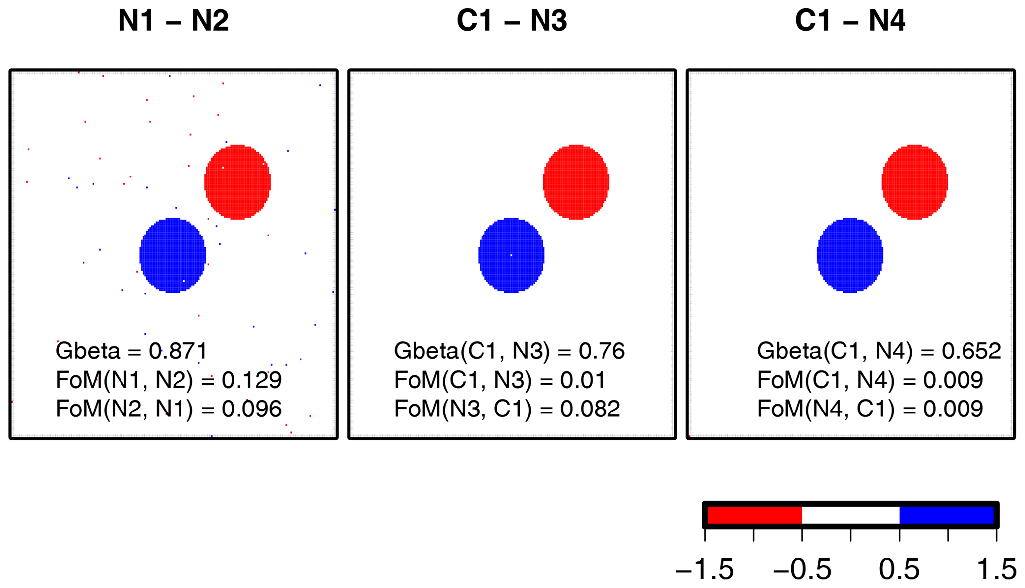
Figure 11 The noisy cases from Gilleland et al. (2020), with results for $G_{{\mathrm{200}}^{\mathrm{4}}/\mathrm{2}}$ and FoM rounded to three decimal places. Images show the difference between each case. Cases N1 and N2 are the same as C1 and C4 but with additional random noise (I_N1(s)=1 and I_N2(s)=1 at randomly chosen s). N3 and N4 are again the same as C4 but with I_N3(s)=1 at $\mathbf{s}=(\mathrm{100},\mathrm{100})$ and I_N4(s)=1 at $\mathbf{s}=(\mathrm{1},\mathrm{1})$.

The latter two noisy comparisons again involve the C1C4 comparison but with a single point of noise added to the C4 field. In the first, the single point is added at the center of C1, and in the last it is added to the lower left corner of the domain. $G(\text{C1},\text{N3})\approx \mathrm{0.76}$ is closer to the value for C1C4 and is nearly identical for C1N4. All of the measures applied in Gilleland et al. (2020) were fairly sensitive to this noise, which is positioned far away from any other nonzero grid point. Because of the differences in scale, the measured effect cannot be compared, but both 0.76 and 0.65 are reasonably close together on the zero to one scale. Moreover, differentiating between the two fields is desired, but it is important to note the size of the difference relative to the error.

FoM is also applied to these comparisons, and while it ranks them the same as G_β (i.e., N1N2 has the highest value followed by C1N3 and C1N4, resp.), it suggests a very poor match between each set of comparisons. It also gave a low grade to the C1C4 comparison, and the value changes in the same direction as for G_β but only very slightly, as it was already very close to zero.

5 G_β and G_β,IL applied to real test cases

Figure 5 shows a snapshot of the MesoVICT core case verification set valid on 20 June 2007 at 18:00 UTC. Comparing Fig. 5a and c, it is clear that CMH (Fig. 5d) missed 3 h precipitation in northern Germany and over forecast precipitation in southern Germany, Austria, and a small part of the Czech Republic at this valid time. The circle histogram (Fig. 5b) shows the difference in sorted CMH-modeled 3 h precipitation minus the sorted VERA analysis values binned by the bearing of the grid points associated with these sorted values from VERA to those of CMH using north as reference. The northern misses and southern false alarms stand out with the long petals in the north and south directions. The q–q plot (Fig. 5d) shows a generally good agreement in terms of the distribution of 3 h accumulated precipitation values but with a slight tendency for the CMH to forecast larger values. Finally, the histogram (Fig. 5e) shows the distances between the sorted values, which are generally very far apart, with a high density of distances beyond 500 km.

Figure 6 is the same as Fig. 5 but ends the 3 h period 21:00–24:00 UTC on 21 June. At this valid time, there is considerably more missed 3 h accumulated precipitation covering much of northern Germany, the Czech Republic, and western Poland (the rest of Poland is outside of the domain). It also misses the precipitation found off the coast of, as well as over, Brittany, France. Figure 6b again shows a north–south issue, while the q–q plot (Fig. 6d) reveals that, for this valid time, the forecast is now under-predicting lower values of 3 h accumulated precipitation but otherwise captures the distribution well for values above about 5 mm (3 h)⁻¹. The histogram of distances (Fig. 6e) between sorted values again shows the long distances between them.

Finally, Fig. 7 shows the same graphic displays but ends the 3 h period 21:00–24:00 UTC on 22 June. CMH again misses precipitation in the north, this time near the easternmost Frisian islands through to the northwestern coast of Germany, and some scattered showers in northern Germany. The circle histogram (Fig. 7b) again shows the north–south bias, but the q–q plot (Fig. 7d) suggests that the model matched the distributional properties of the analysis very well at this valid time. The histogram of distances (Fig. 7e) between sorted values is similar to the previous two valid times.

Much information about forecast performance is provided in Figs. 5 to 7. Subjective analysis of these figures would suggest that the forecast on 20 June is the best, followed by 22 June, with 21 June clearly being the worst. In practice, it is not always possible to diagnose forecast performance with this much detail, and a good summary measure should rank the forecasts valid on these 3 d as a subjective inspection of the graphs in these figures would. Of course, subjective evaluation is also limited, and these summary measures can be useful in identifying problems that are not so easily seen (e.g., Ahijevych et al., 2009; Gilleland, 2017).

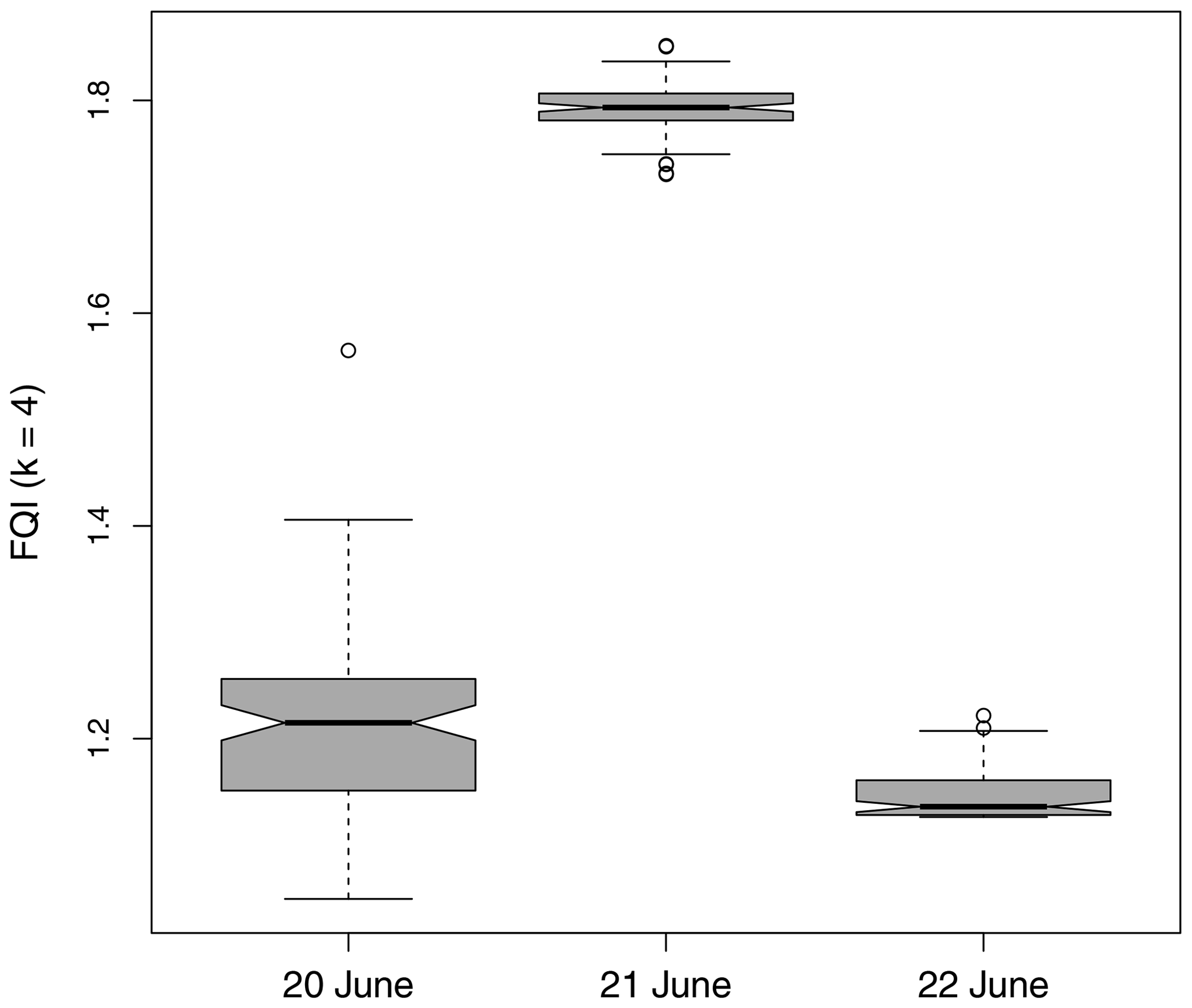
Figure 12 FQI applied to the MesoVICT case 1 12 h lead time forecasts for 3 h accumulated precipitation (in millimeters) ending at 18:00 UTC in 2007 for values above 2 mm (3 h)⁻¹. In each case, 100 FQI (using k=4) values are found using 10 surrogate fields each, and the box plots represent the distribution of FQI values for each set of surrogates.

Figure 12 shows the results after applying the FQI to the core case 3 h accumulated precipitation fields from MesoVICT for values above 2 mm (3 h)⁻¹. Because the FQI involves randomly generated surrogate fields in its calculation, its value will vary each time it is computed. Therefore, 100 values are obtained, using 10 surrogate fields each, in order to obtain a distribution of values. Day 2 is clearly the worst forecast of the 3 d, according to FQI. Day 1 has the most variability but is found to be the second best for most of the 100 iterations, with its 95 % confidence interval (CI) for the median (shown via the notches in each box) clearly not overlapping with the FQI median notches of day 3. The FQI suggests that day 3 is the best forecast day of the three. Subjectively, one might argue that the day 1 is the best, though the forecast did not fare very well in any case. When applied with $\mathit{\beta }=N^{\mathrm{2}}/\mathrm{2}$, G_β,IL is near one, suggesting that the choice of β is too large, which is expected as it is the relatively small spatial areas of intense precipitation that are of interest, and G_β with $\mathit{\beta }=N^{\mathrm{2}}/\mathrm{2}$ is not bothered by such small-scale phenomena. Instead, a much smaller value of β is necessary.

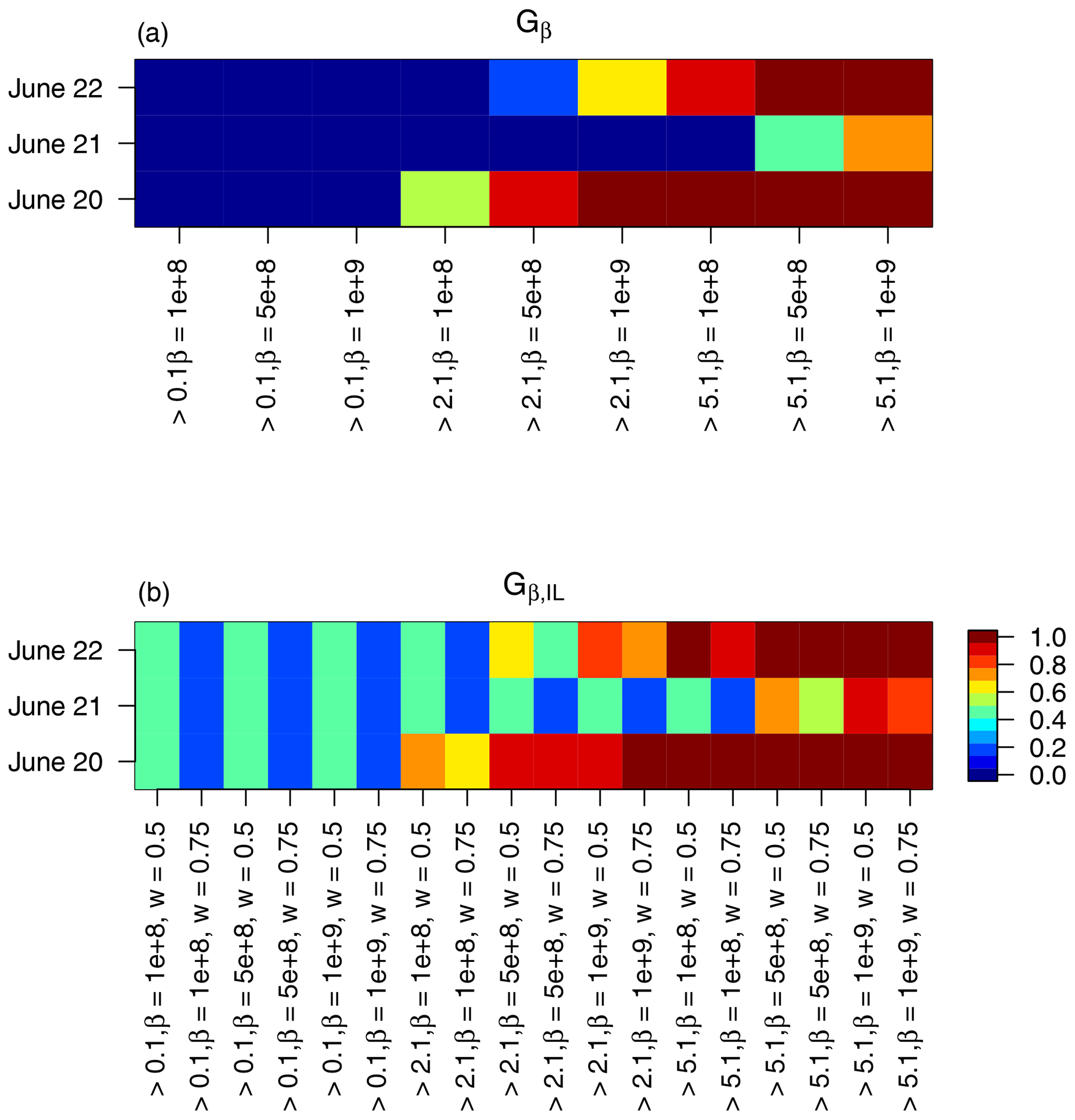
Figure 13 G_β (a), G_β,IL (b) with $\mathit{\beta }=\mathrm{1}\times {\mathrm{10}}^{\mathrm{8}}$, 5×10⁸, and 1×10⁹ and with thresholds of 0.1, 2.1, and 5.1 mm (3 h)⁻¹ applied to the MesoVICT core case.

To ascertain a better choice of β, Fig. 13 shows results for G_β and G_β,IL applied to these same three cases for three different thresholds and choices of β, as well as two choices of weight ($\mathit{\omega }=\mathrm{1}/\mathrm{2},\mathrm{3}/\mathrm{4}$) for G_β,IL. In fact, using the logic of choosing β to be on the scale of the phenomena of interest, G_β=0 and G_β,IL simply give the resulting correlation of the sorted values within the threshold excess areas multiplied by 1−ω. Such low values for these fields should be desired. Nevertheless, the results shown in Fig. 13 are for much larger choices of β in order to give a sense of the sensitivity in choosing this parameter. The value of $N^{\mathrm{2}}/\mathrm{2}$ for these fields is of the order of 800 million, so the choices in Fig. 13 are very large but substantially smaller than $N^{\mathrm{2}}/\mathrm{2}$, and they represent values where, for these types of fields, G_β moves from zero to near one. Both G_β and G_β,IL at these levels of β clearly indicate the poorest performance of the model on 21 June, with a slight preference for the day 1 over day 3, which is arguably consistent with subjective evaluation.

Figure 14 displays the results from applying G_β,IL, $G_{\mathrm{2},\mathit{\beta },\text{IL}}$ (a modification of G_β discussed briefly in Sect. 6.2), and ETS to the 32 ICP real cases. Both of the new measures generally agree with previous results using MODE, image warping, and MED that ARW-WRF has a similar performance to NMM but slightly better. While there are some occasions for the lowest threshold where G_β,IL suggests poor performance for NMM, most show fairly good performance, especially for the two highest threshold choices, which agrees with subjective evaluation and suggests that NMM occasionally has too much scatter that is omitted as the threshold increases. The ETS, on the other hand, suggests close to no skill for both models across the range of values, which is to be expected from a grid-point-by-grid-point type of measure.

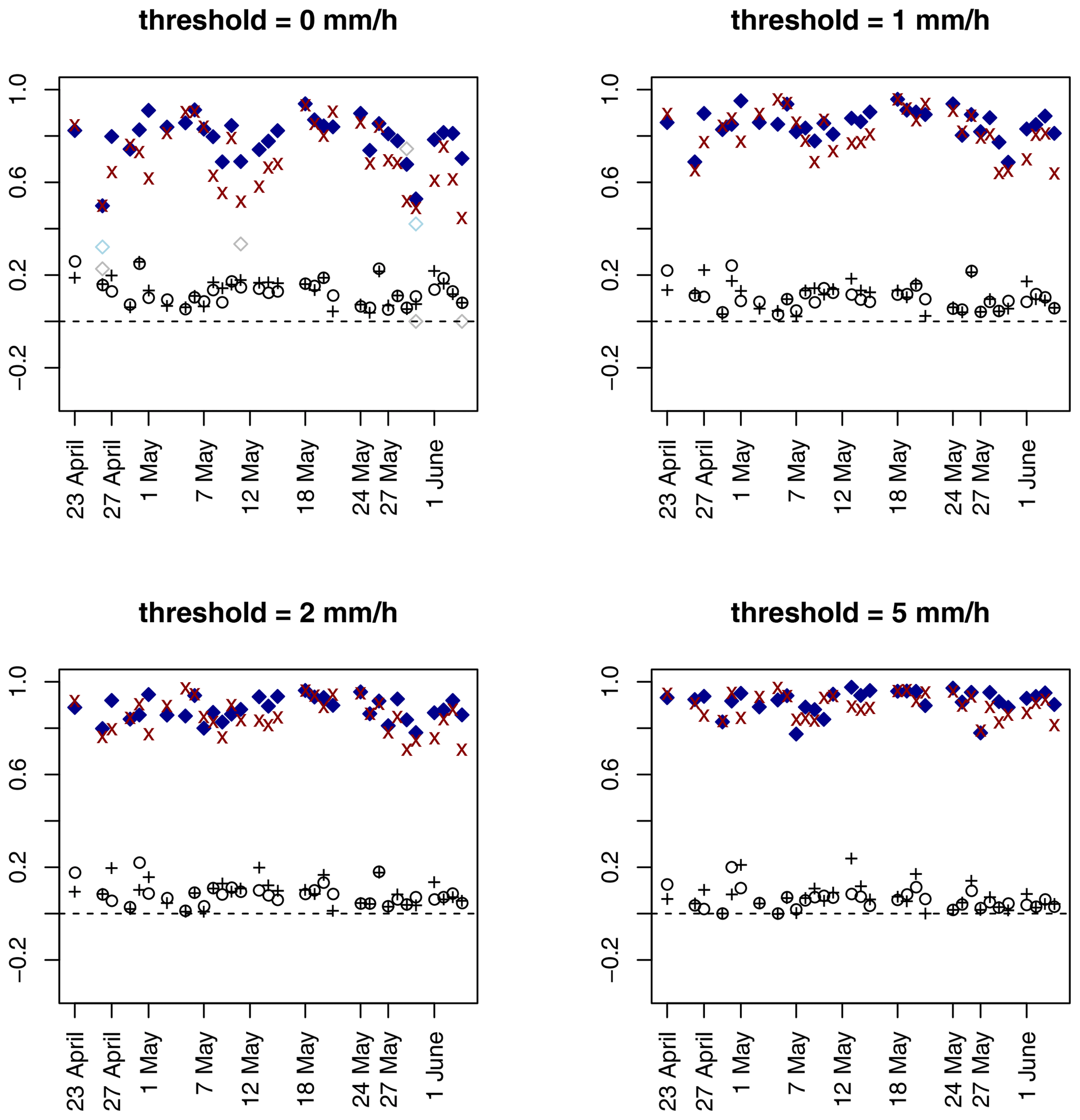
Figure 14 Results from applying G_β,IL, $G_{\mathrm{2},\mathit{\beta },\text{IL}}$ (see Sect. 6.2), and ETS to the 32 ICP real cases. Blue solid diamonds are G_β,IL applied to ARW-WRF, red crosses are for G_β,IL applied to NMM, and open diamonds are $G_{\mathrm{2},\mathit{\beta },\text{IL}}$ applied to ARW (light blue) and NMM (gray). Black + signs are ETS for ARW-WRF, and black circles are ETS applied to NMM. The ordinate axis limits are from $-\mathrm{1}/\mathrm{3}$ to 1, corresponding to the possible range for ETS, and the dashed line provides a visual aid for zero.

Comparing Fig. 14 with Fig. 5 from Gilleland et al. (2010) shows that there is reasonably good agreement between the two methods in terms of which valid times have the best performance and which ones do not and which of the two models is better. The image-warping procedure from Gilleland et al. (2010) is a relatively cumbersome procedure that is difficult to implement in practice, while G_β,IL and $G_{\mathrm{2},\mathit{\beta },\text{IL}}$ are straightforward and efficient to compute. On the other hand, no thresholding procedure is required with the image-warping method.

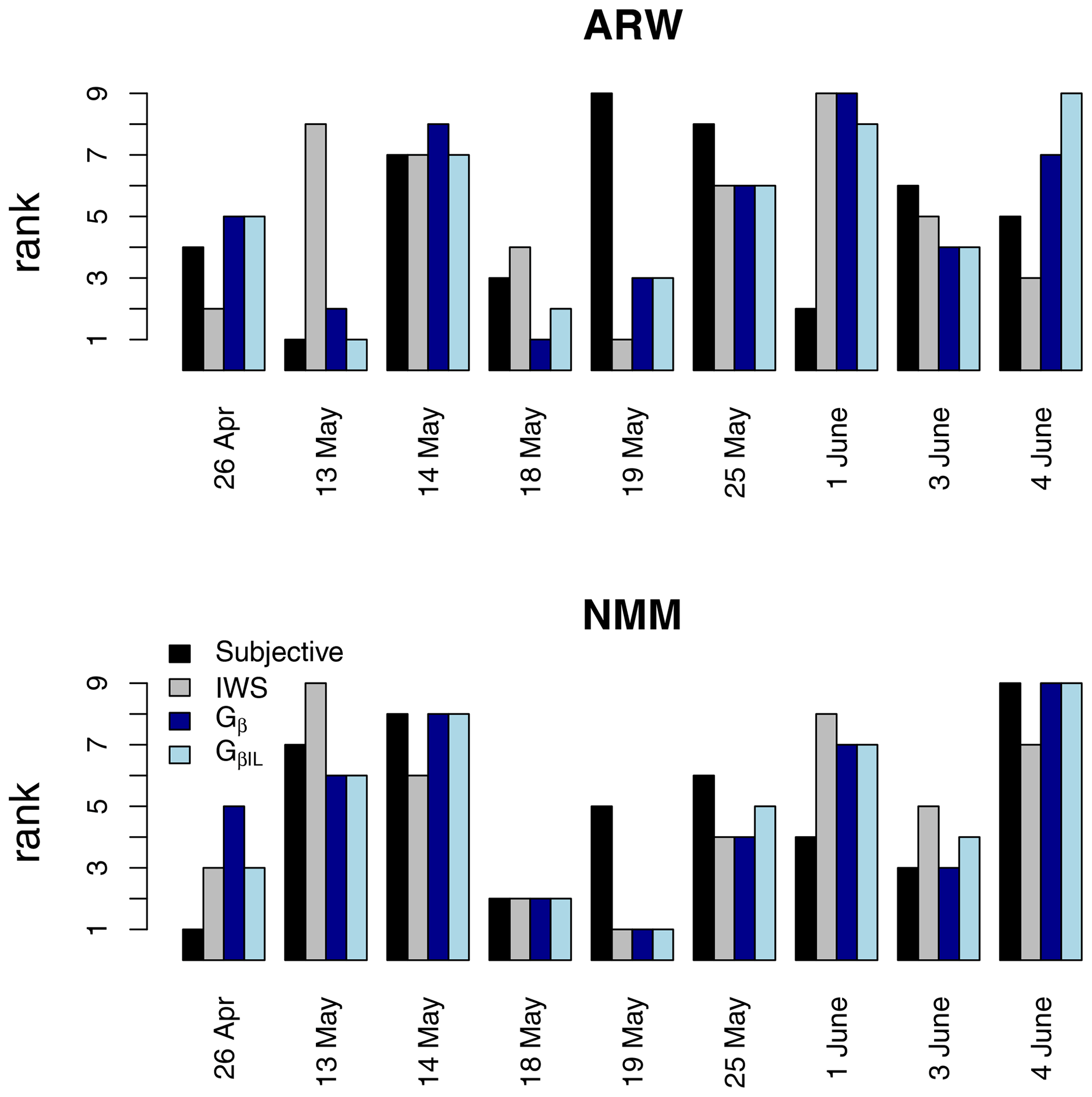
Figure 15 Comparison of the rankings (1 is best and 9 is worst) of the nine ICP real test cases from Ahijevych et al. (2009), including the subjective rankings described therein, and IWS, which is the image-warping score proposed by Gilleland et al. (2010). These cases are a subset of the 32 ICP real cases. A threshold of 2.1 mm h⁻¹ was applied for G_β and G_β,IL. Because the spatial area of precipitation for these cases is relatively small compared to the domain size, $\mathit{\beta }=N/\mathrm{2}$ is used here.

Figure 15 compares rankings for the nine ICP real cases that are a subset of the 32. These cases were introduced and evaluated subjectively in Ahijevych et al. (2009), and they were also evaluated using a summary, called IWS, based on image-warping results by Gilleland et al. (2010). These results are included for comparison with G_β and G_β,IL. The subjective scores cannot be taken as truth, and indeed, there was a large amount of variability among the subjective evaluators' opinions. Rankings for all of these methods are more similar for the NMM model than for ARW. With some notable exceptions, such as 13 May and 4 June for the ARW model, the IWS rankings are fairly similar to those of G_β and G_β,IL.

6 Discussion and conclusions

A total of three new measures are presented, dubbed G, G_β and G_β,IL, which provide meaningful summaries of forecast performance. The first two are spatial alignment and distance based, and the third additionally includes intensity error information in a distributional sense. The latter two measures each range from zero to one, where one represents a perfect match and zero a very poor forecast with the notion of very poor, determined by a user-chosen parameter, β. Desirable properties that have proved challenging for competing measures include that they provide (i) sensible information, even when one or both fields are empty of values, (ii) sensible information, when one or both fields are mostly empty of values, and (iii) information that is not overly sensitive to noise.

Although considerable effort has been made to rigorously test G and G_β, tests for G_β,IL, here, are less rigorous and should be seen as evidence that the measure provides reasonable information. Further testing will be necessary to know how well it can inform about forecast performance under all possible situations. Indeed, the intensity portion of the measure sets a low bar for a forecast to pass muster. However, if a single summary is needed, then it seems to perform well. However, G or G_β, combined with the traditional frequency bias, along with a distributional summary of intensity errors (e.g., differences in mean intensity or, better, the Kullback–Leibler divergence; Kullback and Leibler, 1951) provide a relatively comprehensive summary of forecast performance with little complexity and computational efficiency.

Table 3 Summary of the performance of the distance-based measures as informed through testing on the geometric cases from Gilleland et al. (2020). For each column, affirmative answers represent a positive attribute of the measure and negations represent a negative attribute. See the text for a description of each column heading.

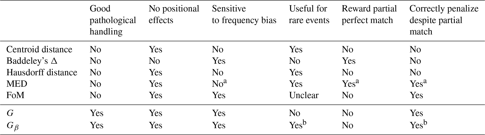
^a MED is an asymmetric measure that provides sensible information for these situations in one direction.
^b With an appropriate choice of β parameter.

Table 3 grossly summarizes the findings in Gilleland et al. (2020) for some of the measures tested there and for G and G_β. Each column specifies an attribute, where an affirmative answer is a positive and a negation is a negative for the measure. The first column refers to whether or not the measures behave well for all of the pathological cases. The next column, labeled “No positional effects,” refers to the first five circle cases in which the first three and second two sets A and B are completely identical, apart from their positions within the field. An affirmative answer means that the measure gives the same value for each set of identical cases. The third column refers to the comparison C2C11 as contrasted against any of the first three circle comparisons. An affirmative answer means that the measure provides sensible information for such biases. The “Useful for rare events” column pertains to whether the measure gives a poor grade to the case C13C14 or not. The last two columns refer to the pair of comparisons C6C7, as contrasted with any of the first three comparisons and C1C9 and C1C10, respectively. An affirmative answer in the penultimate column means that the measure gives a higher score to C6C7 than, for example, C1C2. An affirmative answer in the last column means that the measure differentiates between C1C9 and C1C10 rather than yielding the same value. A negation for a measure in both of these last columns is particularly undesirable although one might prefer a negation in the penultimate column for certain applications. That is, the error part of C6C7 is identical to the error in C1C9, and the partially correct part of C6C7 could be contrasted with the correct negatives in C1C9 (they are both correct in this same region). Therefore, a negation in the last column seems to be the more egregious error.

As can be quickly surmised from Table 3, the only negatives for G are in the “Useful for rare events” and “Reward partial perfect match” columns. The latter is the only negative among these attributes for G_β, where, again, a careful choice of β is necessary in order to be useful in this setting. In terms of the handling of comparison of C6C7 versus C1C2, the measure gives the same result. Thus, it does not give an extra reward for having obtained a perfect match in another part of the field. Thus, the measure will penalize for any defect in the field.

The fact that G is not useful for rare events is by design. The construction of both G and G_β is made with the aim of handling the pathological cases, while still providing sensible information for most situations, which has clearly been accomplished. The rare-event situation is not the focus, although G_β is useful in this setting, provided an appropriate choice of β is used as described in the text. Moreover, the one situation in which the Hausdorff distance is particularly useful is the “rare event” setting so that it can provide complementary information to the measures introduced here.

6.1 Some thoughts about intensity information in spatial verification

The intensity summary suggested, here, for G_β,IL is based on the distribution of errors so that, in particular, it is possible to obtain a perfect score when the two fields are not identical. The MesoVICT core case studied here shows an example in which any distributional measure for intensities is meaningless because the areas of intensity are separated by far too much distance. Therefore, the summary is not entirely satisfactory. It is meaningful when the spatial alignment of errors is much closer, and G or G_β can be used to help inform about the existence of such an issue.

Despite the fact that many methods have been proposed for solving the issue of double penalties and the over-accumulation of small-scale intensity errors, most of these methods do not directly assess intensity information. Most of them target intensity only indirectly through a thresholding procedure, like the one described in Sect. 1.1 and applied here. For example, the fractions skill score (Roberts and Lean, 2008) applies a smoothing filter to binary fields obtained through the threshold process in order to obtain information about frequency of occurrence within neighborhoods of points. Similarly, the intensity-scale skill score (Casati et al., 2004) applies a wavelet decomposition to the verification sets after a fair amount of processing, including reducing the fields to binary fields via thresholding before applying the wavelet decomposition. Other filter-based approaches smooth the intensity values before summarizing the performance, which is also unsatisfactory. Similarly, measures like FQI incorporate only distributional information about the intensities.

The feature-based approach proposed in Davis et al. (2006a, b, 2009) also applies a thresholding process but maintains the intensity information within features. However, the intensity performance is also only incorporated in the final analysis through distributional values, usually in the upper quartile of intensities within a spatial feature. Because these comparative summaries are applied to individual features within the fields, MODE can be thought of as a crude deformation approach, so that its distributional summaries are more satisfactory (e.g., the gross errors of the MesoVICT core case will be correctly handled).

The issue with assessing forecast performance in terms of the intensities stems from the inability to apply a grid-point-by-grid-point accounting of their errors. Once the requirement that their precise locations be used is lifted, then it becomes less clear which values should be compared. Subsequently, thresholding, smoothing, and distributional summaries of intensity performance are the most relevant solutions, and much work has focused on accounting for their spatial alignment errors instead.

One of the earliest methods proposed for verifying forecasts spatially is based on deformations (see Gilleland, 2013, and references therein). G_β, and more so G_β,IL, can be thought of as potentially optimistic image warp results. In particular, the method presented in Gilleland et al. (2010) tries to optimize an objective function that penalizes for translations that are non-physical or too long. G_β and G_β,IL summarize how much lack of overlap there is,and, on average, the distance of any lack of overlap. Thus, if everything could be perfectly aligned (the potential with or without the need for non-physical deformations), then it provides a summary of how much deformation might be required to do so. G_β,IL summarizes the intensity errors in a similar way to the warping procedure of Gilleland et al. (2010) through a distributional measure over the sorted values from each field only (i.e., a perfect match). They are optimistic because they do not consider what it might take to actually realign the fields, and it is possible that no physically meaningful realignment is possible.

Letting RMSL₀ be the root mean square loss (RMSL)³ calculated grid point by grid point in the traditional manner, and RMSL₁ the RMSL calculated over the sorted values only (this time it includes all grid points in each field), then, in the following:

$$\begin{array}{}\text{(5)}& {\displaystyle }{\displaystyle \frac{{\text{RMSL}}_{\mathrm{0}}-{\text{RMSL}}_{\mathrm{1}}}{{\text{RMSL}}_{\mathrm{0}}}}\times \mathrm{100}\end{array}$$

would be the potentially perfect percent reduction in RMSL analogous to that defined in Gilleland et al. (2010) and would represent an upper bound on the error reduction percentage capable of being achieved by the image-warping procedure. This percent reduction in error is analogous to Eq. (2) from Mittermaier (2014) but where the reference RMSL is RMSL₀. It is possible for a forecast to match the observation in intensity values perfectly, even if they are not located at precisely the same grid point locations, so that y₃=0. Indeed, a report of each of RMSL₀, RMSL₁, and the percent reduction in RMSL is a reasonably satisfactory summary of the intensity performance because it informs about the importance of displacement errors. Ebert and McBride (2000) apply translation-only deformations to individual features within the verification sets and summarize the RMSL similarly, as in Eq. (5), but where they are able to break it down into RMSL attributed to total, displacement, volume, and pattern types of errors. Such a breakdown is attractive but the processing involved to obtain them is considerable.

Another issue about summarizing intensity information is that many forecasts are first calibrated before applying any verification so that the intensity values should be fairly close in a distributional sense. Therefore, measures that include intensity components like those suggested here, i.e., FQI and MODE, among many others, will generally not be affected much by the intensity terms in their equations. Subsequently, the summaries proposed herein represent highly efficient, interpretable, and sensible summaries that provide a useful alternative.

6.2 Potential modifications to the proposed summary measures

A possible generalization of G_β (G_β,IL) that would allow a user to weight each component of y from Eq. (3) differently would be to replace y₁ and y₂ with $y_{\mathrm{1}}^{{\mathit{\gamma }}_{\mathrm{1}}}$ and $y_{\mathrm{2}}^{{\mathit{\gamma }}_{\mathrm{2}}}$. However, an initial investigation of implementing this additional complexity in G_β found the measure to be highly erratic for small changes in γ₁ and γ₂, making it difficult to obtain an interpretable measure.

Another possible modification to G_β is to introduce an additional user-chosen parameter $\mathrm{0}\le \mathit{\alpha }<\mathit{\beta }$ in the following manner:

$$\begin{array}{}\text{(6)}& {\displaystyle }{\displaystyle }{G}_{\mathit{\alpha },\mathit{\beta }}(A,B)=max\left\{\mathrm{1}-{\displaystyle \frac{y-\mathit{\alpha }}{\mathit{\beta }-\mathit{\alpha }}},\mathrm{0}\right\}.\end{array}$$

The effect is to allow for a perfect score for a model that is very close to the observation but not a perfect match. It could be thought of as an adjustment for errors that are not considered important. In fact, G_β given in Eq. (3) is the same as Eq. (6) but with α=0.

Another modification that is similar to G_β,IL, denoted here by $G_{\mathrm{2},\mathit{\beta },\text{IL}}$, modifies Eq. (3) through the y term as follows:

$$\begin{array}{}\text{(7)}& {\displaystyle }{\displaystyle }{G}_{\mathrm{2},\mathit{\beta },\text{IL}}(A,B)=max\left\{\mathrm{1}-{\displaystyle \frac{y_{\mathrm{1}}{y}_{\mathrm{2}}(\mathrm{1}+y_{\mathrm{3}})}{\mathit{\beta }}},\mathrm{0}\right\},\end{array}$$

where y₁ and y₂ are as in Eq. (3), and y₃ is the mean absolute loss (MAL) between the sorted original values at locations within the sets A and B. The RMSL (as in Rezacova et al., 2007) could be used in the place of MAL if applying a greater penalty for large intensity differences is desired. If y₃=0, then $G_{\mathrm{2},\mathit{\beta },\text{IL}}$ reduces to G_β. Otherwise, the measure provides an additional penalty for a lack of distributional agreement in the intensities.

Figure 14 displays results for this modification along with those for G_β,IL, and it can be seen that the results are similar for both measures, apart from a few cases where the multiplication of the intensity term causes a more drastic penalization of the forecasts than G_β,IL (top left panel). A difficulty with $G_{\mathrm{2},\mathit{\beta },\text{IL}}$ is that the multiplication of the intensity term in Eq. (7) makes choosing β more difficult because the intensity loss information may depend on the specific variable of interest, and the units for y₃ will generally differ considerably from y₁ and y₂.

The summary measure, y, in both G_β and G_β,IL, passes the requirements to be a true mathematical metric. $max\mathit{\{}\mathrm{1}-y/\mathit{\beta },\mathrm{0}\mathit{\}}$ simply rescales the metric to be between zero and one and reorients it so that one, instead of zero, corresponds to a perfect match. Gilleland (2017) argued in favor of the violation of the symmetry property for the mean error distance (MED) because information about misses and false alarms can be inferred. G_β can be modified to be asymmetric in this way by only including one of the MED terms in the y₂ term of Eq. (3) and by removing one of the n_A or n_B terms from y₁; that is, an asymmetric $G_{\mathit{\beta }}^a(A,B)$ would have $y_{\mathrm{1}}^a=n_B-n_{AB}$ and $y_{\mathrm{2}}^a=\text{MED}(A,B)\cdot n_B$.

The building blocks for G_β and G_β,IL themselves make for a good summary vector for forecast performance. For example, knowledge of n_A, n_B, n_AB, MED(A,B), MED(B,A), and, in the case of non-binary fields, y₃ with MAL or RMSL calculated over the areas A and B, without first sorting them, provides a wealth of diagnostic information about forecast performance. Examples include which component(s) contributed most to a particular G_β or G_β,IL value, the frequency bias, the average distance from observed areas of activity to those that were forecast (and vice versa), and the potential and actual intensity error in addition to the percent reduction in error possible if the forecast field could be perfectly realigned with the observation field.

The proposed measures are designed for 2D spatial fields here, but because of the simplicity of the measures, they can be easily extended to any number of dimensions. For example, a third dimension of time could be added in order to verify an entire spatiotemporal verification set with a single summary number. Such a scheme would provide limited information, but it would nevertheless provide a simple summary that would allow for a ranking between competing gridded forecast models over numerous time points. Many variables also have an important vertical component so that the measures could be extended for the horizontal and vertical dimensions. Additionally, although the analysis here is focused on gridded verification sets, the measure can be extended to a verification set where both spatial fields are irregular point locations. Further study would be needed to investigate these applications, both in terms of their behavior in these settings and their feasibility in terms of computational efficiency.

Spatial forecast verification is only one avenue in which the measures introduced here can be applied. For example, G could be especially useful as the loss function when predicting a spatial-exceedance region as in Zhang et al. (2008); Cressie and Suesse (2020).