A generalized Spatio-Temporal Threshold Clustering method for identification of extreme event patterns

Extreme weather and climate events such as floods, droughts, and heat waves can cause extensive societal damages. While various statistical and climate models have been developed for the purpose of simulating extremes, a consistent definition of extreme events is still lacking. Furthermore, to better assess the performance of the climate models, a variety of spatial forecast verification measures have been developed. However, in most cases, the spatial verification measures that are widely used to compare mean states do not have sufficient theoretical justification to benchmark extreme events. In order to alleviate inconsistencies when defining extreme events within different scientific communities, we propose a new generalized Spatio-Temporal Threshold Clustering method for the identification of extreme event episodes, which uses machine learning techniques to couple existing pattern recognition indices with high or low threshold choices. The method consists of five main steps: (1) construction of essential field quantities; (2) dimension reduction; (3) spatial domain mapping; (4) time series clustering; and (5) threshold selection. We develop and apply this method using a gridded daily precipitation dataset derived from rain gauge stations over the contiguous United States. We observe changes in the distribution of conditional frequency of extreme precipitation from large-scale well-connected spatial patterns to smaller-scale more isolated rainfall clusters, possibly leading to more localized droughts and heat waves, especially during the summer months. The proposed method automates the threshold selection process through a clustering algorithm and can be directly applicable in conjunction with modeling and spatial forecast verification of extremes. Additionally, it allows for the identification of synoptic-scale spatial patterns that can be directly traced to the individual extreme episodes, and it offers users the flexibility to select an extreme threshold that is linked to the desired geometrical properties. The approach can be applied to broad scientific disciplines.

1 Introduction

Extreme events of essential climate variables (Bojinski et al., 2014) such as heavy rainfall, high temperatures, and strong winds and their derivatives such as droughts and heat waves are a major source of risk to society and the environment. The purpose of risk management is to design and implement a set of common procedures for predicting, measuring, and managing such high impact events. The critical step is how to identify these extreme processes. However, there is no uniformly accepted definition of extreme events. More often than not, the process of identifying extreme events has been typically based on classifying them into groups with characteristics such as frequency of occurrence, intensity, temporal duration, and timing (Stephenson, 2008). In addition, the evaluation of the multidimensional nature of extreme events, in most cases, has been confined to individual grid points or stations, thus overlooking embedded spatial dependency. The Intergovernmental Panel on Climate Change (IPCC) defines a climate extreme as “the occurrence of a value of a weather or climate variable above (or below) a threshold value near the upper (or lower) ends of the range of observed values of the variable” (IPCC, 2012). Typically, the choice of a high (or low) threshold depends on the conventions of specific scientific disciplines. For example, the climate science community tends to select location-specific thresholds based on either categories (e.g., Sun et al., 2007; Dai, 2001; Dai et al., 2017), quantiles (e.g., Groisman et al., 2005; Lau et al., 2013; Pendergrass and Hartmann, 2014), combinations (e.g., Kunkel et al., 2003, 2007, 2010, 2012), or indices (e.g., Alexander et al., 2006; Zhang et al., 2011; Donat et al., 2013a, b). Hereafter, we refer to these selection methods as conventional location-specific threshold (CLST) methods.

In the realms of statistical modeling, under appropriate conditions, excesses above (below) a high (low) threshold are often modeled using the generalized Pareto distribution (GPD) (Balkema and de Haan, 1974; Pickands, 1975), where the requirement for a chosen threshold is to be high (low) enough to satisfy a chosen goodness-of-fit test. Although threshold choices often overlap across disciplines, it is still difficult to compare extreme value analysis results between different scientific studies if the threshold selection methodologies differ. Even when the same forecast verification strategy is used (e.g., Jolliffe and Stephenson, 2003; Wilks, 2011, chap. 8), the results will be different. Thus a unified approach for threshold selection (i.e., universal extreme event definition) is essential because it standardizes the inference process for extreme event analysis, leading to further consistency and transparency when comparing results between different scientific findings. Unification, standardization, and transparency are the key pillars of disciplined risk management.

While many univariate methods have been proposed to automate the threshold choice (e.g., Fukutome et al., 2015; Scarrott and MacDonald, 2012; Bader et al., 2017), there are no clear-cut criteria, and in practice, threshold choice tends to be determined by either exploration methods or by stability assessments of parameter estimates, and in most cases, the threshold selection is disconnected from the geometrical properties of the desired spatial field. Here, we express geometrical properties by geometric attributes that measure the texture/dispersiveness of the spatial field. Ultimately, the choice of threshold is always an interplay between bias and variance (Smith, 1987). For high extreme thresholds, if the chosen threshold is not high enough, the GPD likely will not have a good fit to the excesses above the threshold, leading to approximation bias. Conversely, if the chosen threshold is too high, only a small number of exceedances will be generated, and consequently, there will be high variance in the estimators (in the case of low extreme thresholds, these conditions are reversed). A more comprehensive evaluation of univariate extreme value theory (EVT) is given in Coles (2001).

Analysis of extreme events must also incorporate the spatial nature of the key climate variables since many single quantities, such as precipitation or temperature, are measured at multiple locations that may also be teleconnected via atmospheric circulations or hydrological cycles. Implementation of spatial extreme value analysis has to be done using an integrative modeling approach (IMA), in which different scientific disciplines are combined into one holistic process, joined by a common modeling factor(s) subject to uniform assumptions. For example, in statistics, it may involve the integration of multivariate EVT (e.g., Cooley et al., 2012), geostatistics (e.g., Banerjee et al., 2015), and spatial forecast verification (e.g., Friederichs and Thorarinsdottir, 2012), and in atmospheric science, it would encourage the use of high-resolution climate models (e.g., to resolve localized extreme events) combined with a spatio-temporal threshold selection algorithm and multivariate EVT to capture spatial dependencies. While a myriad of other coupling combinations is possible, the challenging aspect of this integration lies in maintaining suitable and consistent statistical assumptions across all modeling blocks.

This paper proposes a new generalized Spatio-Temporal Threshold Clustering (STTC) method for extreme events within the IMA framework. By generalized, we mean the algorithm's applicability to the wide variety of essential climate and non-climate variables (e.g., air pollution, crop yield, streamflow) and their derived quantities, hereafter essential field quantities (EFQs). The algorithm, as objectively as possible, detects large-scale extreme spatial patterns that occupy fairly extensive geographical areas. Those patterns contain extreme fields (i.e., for high or low extreme thresholds, only fields from the respective upper or lower quantile of the distribution are selected) in both temporal and spatial variations. They can be linked to individual extreme episodes such as flash floods, heat waves, hurricanes, and droughts.

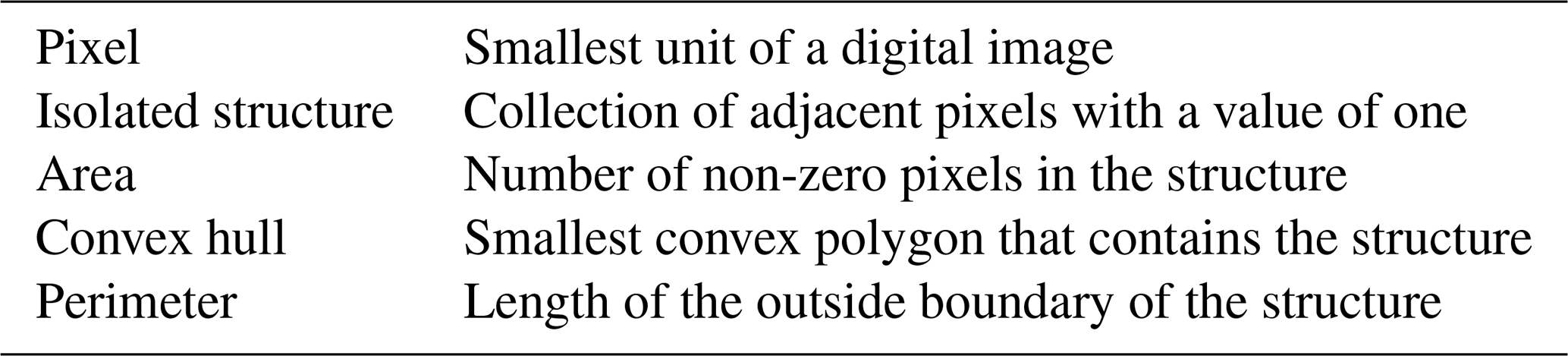
The threshold selection process is conditioned on these extreme patterns and enables one to detect latent spatial dependencies with the help of geometric indices from digital topology. Furthermore, to evaluate areas with the largest conditional frequency values, we apply the STTC methodology that uses a time series clustering procedure for a number of geometric indices. This procedure facilitates the algorithm's ability to classify a spatial pattern of an image (e.g., the conditional frequency of positive or negative extreme EFQ) by several geometrical constructs described in Table 1. As far as we are aware, this machine learning IMA is a new contribution in atmospheric science that links the threshold selection process conditioned on extreme patterns with the clustering of multivariate series of geometric properties.

Table 1 Geometrical constructs used in geometric indices.

The remainder of the paper is structured as follows. Section 2 reviews the conceptual framework and details all steps for the STTC algorithm. Section 3 describes the dataset for illustrating the algorithm development and evaluation. Section 4 and its subsections present underlying methods. Section 5 highlights an outcome of the clustering algorithm and comparative analysis utilizing daily precipitation data and underlines essential findings. Section 6 gives the conclusions.

2 Conceptual framework

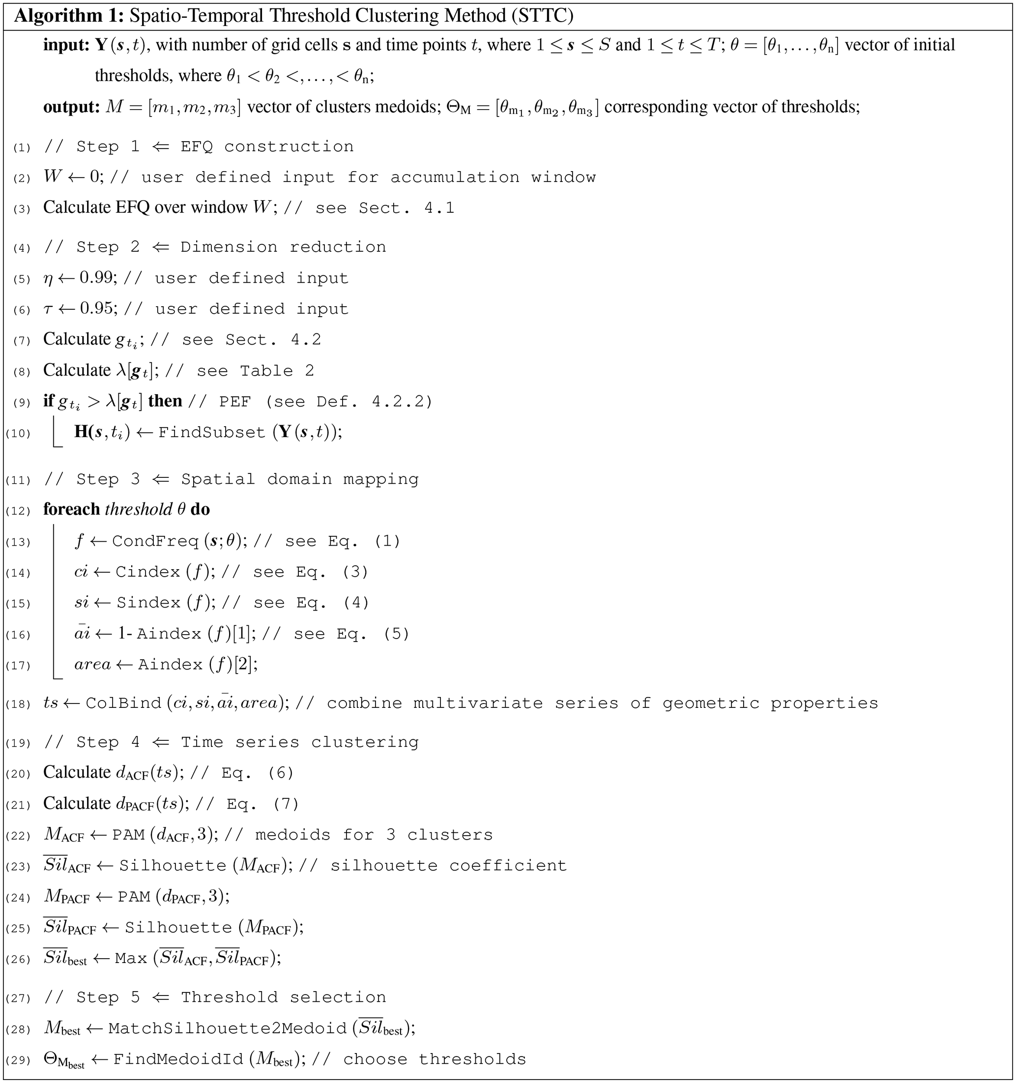
The STTC algorithm consists of five main steps:

1. EFQ construction closely matched to the timeframe of interest;

2. dimension reduction based on statistical quantiles;

3. spatial domain mapping represented by the geometric indices;

4. time series clustering applied to the multivariate series of geometric properties; and

5. threshold selection linked to the time series clustering.

The first step is the most flexible and difficult to apply. The user must decide whether to convert (e.g., normalize, standardize) the raw data to best represent an extreme pattern of interest. Large-scale patterns are usually described by gridded data, such as precipitation, temperature, geopotential height, or vorticity, to name a few. The patterns can be analyzed either at the right or left tail of the distribution. Ultimately, the choice of EFQ is based on the problem at hand and individual user preference.

Next, the dimension reduction or conditioning step identifies extreme processes that are spread out over a relatively extended portion of the spatial domain. This step is necessary to narrow spatio-temporal space to fit the class of events of interest. For example, the conditioning can be performed utilizing the algorithm to find either positive (i.e., wet-day) or negative (i.e., dry-day) extreme fields. Rather than considering extreme values at individual locations and their temporal dependence, we consider an overall spatial field that is conditioned on being extreme (i.e., not all individual grid cells within the field have to be extreme). In this case, it is possible to depict large-scale spatial extreme patterns independent of whether or not individual grid cells in space are extreme. The concept is similar to the high field energy used to identify severe storm environments in Gilleland et al. (2013, 2016). They used the product of the 0–6 km wind shear and maximum potential wind speed of updrafts and selected its upper quartile in space greater than its 90th percentile over time to define the high field energy. Here we adapt this framework of first identifying data-specific quantile in space (i.e., the quantile function is applied over entire spatial domain) and then in time. We also replace the concept of high field energy with more general positive and negative extreme fields (see Sect. 4.2) that can accommodate a variety of extreme field definitions, including different quantile values to meet the specific needs of different datasets.

The classification and evaluation of the graphical properties of the spatial fields, depicted in the previous step, are the purpose of the spatial domain mapping phase of the algorithm. The user selects a vector of initial thresholds where evaluation takes place. The threshold selection framework is integrated with methods from digital topology. Values greater or equal than a chosen threshold are assigned to one, and values below to zero. It is called image digitizing and is a widely used technique in computer imaging. The digitized image then can be mapped to several geometric attributes that represent a particular graphical property of the image. As the threshold varies, so do the values of the geometric attributes. As such, one can create a threshold series that is mapped to the corresponding multivariate series of geometric properties. The mapping process can be repeated for all geometric attributes, creating a non-linear dependence between the threshold series and the desired geometrical properties.

The fourth step of the algorithm consists of applying time series clustering to the multivariate series of geometric properties derived in the previous step. This unsupervised machine learning approach separates the multivariate series of geometric properties into individual clusters by minimizing the average dissimilarity between each cluster's centrally located representative object and any other object in the same cluster. Each of these representative objects is associated with a specific threshold from the threshold series.

The last threshold selection step selects a threshold out of the threshold series based on the clustering analysis of the multivariate series of geometric properties. The position of the representative object in the multivariate series of geometric properties is then matched to the same position in the threshold series, producing a cluster-specific threshold.

Thus, the overall objective of the algorithm is to detect latent spatial dependencies for an EFQ of interest within large-scale extreme episodes and to automate threshold selection for the extreme spatio-temporal processes. Ultimately, the identified spatial extremes can be linked to individual weather patterns because the corresponding occurrence times of such extreme events are tracked during the identification process. The objective threshold choice for extreme event modeling can help to deepen our understanding of the underlying processes in forming those patterns, that were possibly overlooked in the CLST methods. The STTC algorithm incorporates spatial and temporal dependencies in one holistic modeling framework and enables future spatio-temporal analysis of extreme events based on either a single quantity (e.g., precipitation) or a composite index of multiple quantities (e.g., the Palmer Drought Severity Index). Moreover, the extreme threshold value that was estimated through the unsupervised machine learning approach and the resultant extreme spatial field can be further incorporated into a spatial forecast verification process or independently applied in statistical modeling utilizing multivariate EVT. The use of this method can thus ensure consistency between the extreme threshold values and spatial fields selected during the modeling and forecast verification steps. A detailed summary of the entire STTC algorithm can be found in Appendix A.

3 Data

To illustrate the algorithm development and evaluation, we consider station-based precipitation measurements in millimeters per day obtained from the Global Historical Climatology Network-Daily (GHCN-Daily; Menne et al., 2012a) collected over the period from 1 January 1961 to 31 December 2016 (56 years). While the GHCN-Daily dataset was subject to a rigorous quality assurance procedure (Menne et al., 2012b), it was not adjusted for artificial discontinuities such as changes in station location, instrumentation, and time of observation (Donat et al., 2013b). To deal with these issues, we only select stations with at least 40 % data coverage, yielding 8516 stations. In addition, as described in Liang et al. (2004), we perform topographical adjustments to account for the strong elevation dependence of the rain gauge sites by using the Parameter-Elevation Regression on Independent Slopes Model (PRISM) (Daly et al., 1994, 1997). We then interpolate the GHCN-Daily dataset using the Cressman objective analysis scheme (Cressman, 1959) to a 30 km by 30 km grid covering the contiguous United States (CONUS). As a result, we obtain approximately 27 000 spatial points, with each point having over 20 000 days of temporal rainfall coverage.

4 Methods

4.1 EFQ construction

A fundamental decision in any extreme value analysis is to choose the types of extreme events to analyze (e.g., flash floods, persistent droughts, or other natural disasters). Depending on the choice, our algorithm allows adjustment of an accumulation window (W). The proposed EFQ derivation involves several steps, which can be modified or entirely skipped depending on a specific application.

1. Remove seasonal patterns by subtracting climatological mean values over the entire time length from the raw data.

2. Calculate W-period rolling accumulated anomalies.

3. Standardize accumulated anomalies by the corresponding high (or low) temporal quantile.

In this research paper, we select no accumulation window and a high quantile of order 0.95 and use daily precipitation as the field of study. That is, our interest during the algorithm testing lies in short-term extreme rainfall. These short-duration impactful precipitation events can produce a major natural hazard, such as a flash flood in some areas. To illustrate the general application, we also later present examples using more extended Ws for extreme EFQs. By design, EFQ has no units.

4.2 Dimension reduction

Conventional temporal dimension reduction methods such as principal component analysis (PCA) and linear discriminant analysis (LDA), which rely heavily on mean and covariance estimation, are not very informative for extremes. The block-maximum approach is often used to analyze extremes and potentially excludes relevant observations (Coles, 2001). The challenge is, therefore, to subsample a relatively small number of observations to represent the tail of the distribution and to select an aggregate measure that accurately describes extreme events. Gilleland et al. (2013) considered, for this purpose, a conditional frequency with quantile-based dimension reduction methodology in analyzing severe storms. In the present context, we modify this method to apply for temporal and spatial quantile values more appropriate in our case (see Sect. 5). We further formalize this method with the following definitions.

Definition 4.2.1.

Let Y(s,t) be a spatio-temporal EFQ with a number of spatial pixels s∈𝒟, where 𝒟 is the spatial domain; then, at each time point $t=[\mathrm{1},\mathrm{\dots },T]$, the ηth quantile in space y_t,η is given by $\mathbb{P}\mathit{\left\{}\mathbf{Y}\right(\mathit{s},t)\le y_{t,\mathit{\eta }}\mathit{\}}=\mathit{\eta }$, where $\mathit{\eta }\in [\mathrm{0},\mathrm{1}]$.

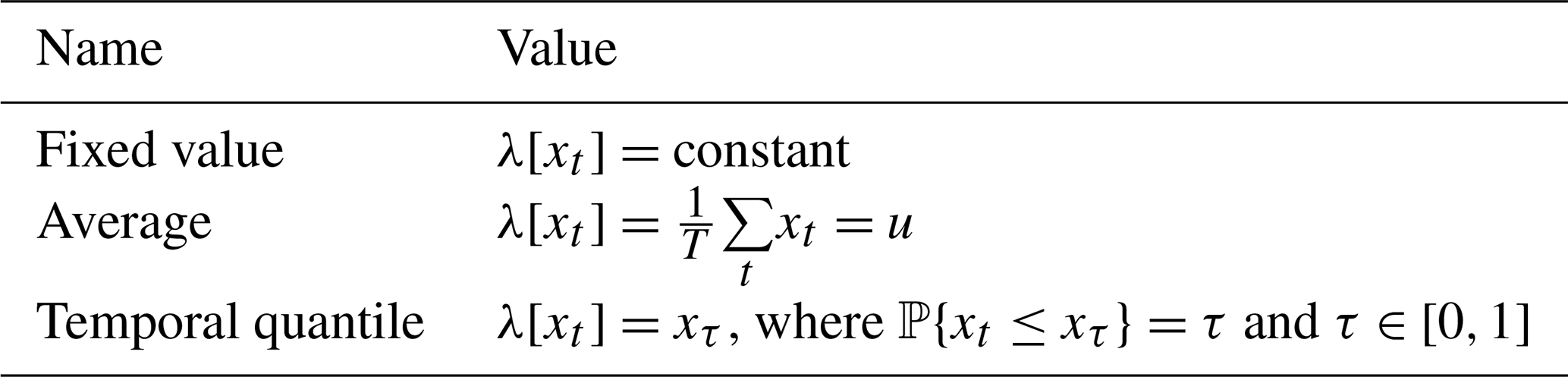
The quantile y_t,η in Definition 4.2.1 is taken over space at each point in time so that a univariate time series of the spatial quantile results. We denote this series by ${\mathit{g}}_t=g_{\mathrm{1}},\mathrm{\dots },g_T=y_{\mathrm{1},\mathit{\eta }},\mathrm{\dots },y_{T,\mathit{\eta }}$. In addition, we introduce a function λ[⋅] with possible forms in Table 2.

Definition 4.2.2.

A space–time process Y(s,t) is called a Positive Extreme Field (PEF) at any time point t_i when {$g_{t_i}>\mathit{\lambda }\left[{\mathit{g}}_t\right],i=[\mathrm{1},\mathrm{\dots },N_H],N_H\mathit{⩽}T$} denote H(s,t_i) to be the subset of Y(s,t) when Y(s,t) is a PEF.

Definition 4.2.3.

A space–time process Y(s,t) is called a Negative Extreme Field (NEF) at any time point t_j when {$g_{t_j}<\mathit{\lambda }\left[{\mathit{g}}_t\right],j=[\mathrm{1},\mathrm{\dots },N_L],N_L\mathit{⩽}T$} denote L(s,t_j) as the subset of Y(s,t) when Y(s,t) is a NEF.

Table 2 Possible forms for function λ[x_t].

The PEF (NEF) concepts are general constructs that can be applicable to both short- and long-term impactful extreme events. For instance, if we express PEF and NEF in terms of precipitation rates and try to detect natural disasters such as documented in the NOAA National Centers for Environmental Information (NCEI) report titled “U.S. Billion-Dollar Weather and Climate Disasters (2018)”, we can identify a multitude of high-profile cases, a few of which are presented in Fig. 1.

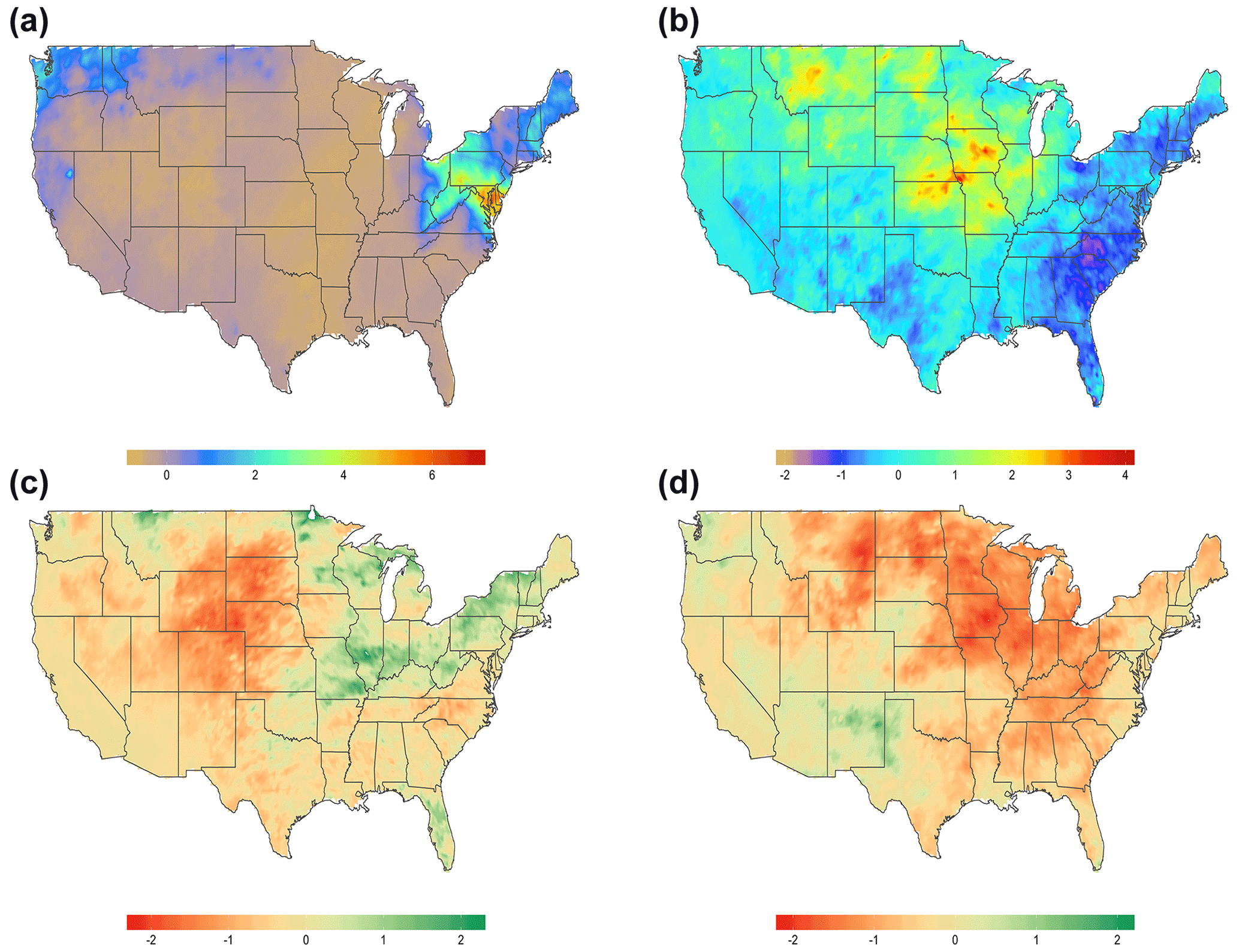
Figure 1 Examples of PEF: (a) October 2012 Superstorm Sandy (W=4); (b) May to October Great Flood of 1993 (W=180). Examples of NEF: (c) 2002 Drought, April–June (W=90); (d) 1988 Drought, March–July (W=150). The PEF and NEF were derived from precipitation measurements obtained from the gridded Global Historical Climatology Network-Daily (GHCN-Daily) dataset (see Sect. 3 for more information) and expressed in terms of standardized anomalies. The function λ[⋅] from Table 2 was set to the temporal quantile definition with η=0.99 for PEF (η=0.01 for NEF) for the univariate time series g_t with τ=0.95 for PEF (τ=0.05 for NEF).

Figure 1a shows Superstorm Sandy, where high PEF values (>6) are observed over the Mid-Atlantic and New England regions and northern Ohio. The Great Flood of 1993, which is found with a much longer accumulation window (W=180), is displayed in Fig. 1b. The areas with PEF >2 can be seen along the Missouri and Mississippi rivers and their tributaries. In addition, several heavy rainfall events are spotted in Montana during the same time period. Results for the drought of 2002 are shown in Fig. 1c. The Rocky Mountains and Midwest regions are particularly impacted by very dry conditions. Figure 1d shows a similar graph but for the 1988 drought and with W=150. The effects of low negative NEF ($<-\mathrm{1}$) are seen in Mid-Atlantic states, the southeastern United States, the midwestern United States, and the western United States. These are all examples of types of extreme processes H(s,t_i) (L(s,t_j)) that define a spatio-temporal subset of a dataset used to define a conditional frequency of extreme EFQ.

The conditional frequency of an EFQ Y(s,t) is given by (i.e., conditioned on) H(s,t_i) and can be defined as a function of high threshold θ_h at any spatial pixel s∈𝒟 in the following way:

$$\begin{array}{}\text{(1)}& f(\mathit{s};{\mathit{\theta }}_{\text{h}})={\displaystyle \frac{\sum _{i=\mathrm{1}}^{N_H}{\text{𝟙}}_{\mathit{\left\{}\mathbf{H}\right(\mathit{s},t_i)>{\mathit{\theta }}_{\text{h}}\mathit{\}}}}{N_H}},\end{array}$$

where 𝟙_{⋅} is the indicator function.

Alternatively, we can delineate a similar quantity but conditioned on L(s,t_j) if a low threshold θ_l is of interest:

$$\begin{array}{}\text{(2)}& f(\mathit{s};{\mathit{\theta }}_{\text{l}})={\displaystyle \frac{\sum _{j=\mathrm{1}}^{N_L}{\text{𝟙}}_{\mathit{\left\{}\mathbf{L}\right(\mathit{s},t_j)<{\mathit{\theta }}_{\text{l}}\mathit{\}}}}{N_L}}.\end{array}$$

In terms of additional notations, let $\mathit{\theta }=[{\mathit{\theta }}_{\text{1}},\mathrm{\dots },{\mathit{\theta }}_{\text{n}}]$ be a set of initial thresholds such as ${\mathit{\theta }}_{\text{1}}<{\mathit{\theta }}_{\text{2}}<,\mathrm{\dots },<{\mathit{\theta }}_{\text{n}}$. We can think of the series $f(\mathit{s};{\mathit{\theta }}_{\text{1}}),\mathrm{\dots },f(\mathit{s};{\mathit{\theta }}_{\text{n}})$ as a procedure of partitioning the conditional frequency image into several overlapping homogeneous fields, where each field is mapped into the corresponding geometric properties series described in the next section.

4.3 Spatial domain mapping

Geometric indices employed here were first introduced by AghaKouchak et al. (2010) and applied to validate radar data against satellite precipitation estimates and weather prediction models. Gilleland (2017b) complemented geometric indices with mean-error and mean-square-error distances, to introduce new diagnostic plots within a spatial forecast verification framework. The diagnostics were applied to a number of cases from the spatial forecast verification intercomparison project (ICP, http://www.ral.ucar.edu/projects/icp, last access: 13 April 2021) (Ahijevych et al., 2009; Gilleland et al., 2009, 2010). The indices vary between zero and one and describe the connectivity, shape, and area of the image pixels for a predefined threshold. The connectivity index is defined as

$$\begin{array}{}\text{(3)}& C_{\text{index}}=\mathrm{1}-{\displaystyle \frac{n-\mathrm{1}}{\sqrt{m}+n}},\end{array}$$

where n is the number of isolated structures, and m is the number of pixels with a value of one (i.e., above a chosen threshold). Here, an isolated structure is a group of adjacent non-zero pixels. The connectivity index shows how the structures within the image are interconnected. The higher (lower) the index, the more connected (dispersed) the fields are within the image. The shape index is given by

$$\begin{array}{}\text{(4)}& S_{\text{index}}={\displaystyle \frac{P_{\text{min}}}{P}},\end{array}$$

where P is the perimeter of the pixels above a given threshold, and P_min is the theoretical minimum perimeter of an m-pixel pattern, which is attained if the pattern of non-zero pixels was formed closest to a perfect circle. Mathematically, it is defined as

$$P_{\text{min}}=\left\{\begin{array}{ll}\mathrm{4}\times \sqrt{m},& \text{if}\lfloor \sqrt{m}\rfloor =\sqrt{m}\\ \mathrm{2}\times \left(\lfloor \mathrm{2}\times \sqrt{m}\rfloor +\mathrm{1}\right),& \text{otherwise}\end{array}\right.,$$

where ⌊⋅⌋ is the floor function. The near-one values of S_index imply an approximately circular pattern of non-zero pixels. For a more detailed discussion about these indices, see Gilleland (2017b). Finally, to measure object complexity, we introduce another geometric index defined in Bullock et al. (2016) as follows:

$$\begin{array}{}\text{(5)}& {\overline{A}}_{\text{index}}=\mathrm{1}-A_{\text{index}}\equiv \mathrm{1}-{\displaystyle \frac{A}{A_{\text{convex}}}},\end{array}$$

where A is the area of the pixels (i.e., the number of non-zero grid points) above a given threshold, A_convex is the area of the convex hull around those pixels, and A_index is defined as their ratio. The index values close to zero are representative of more structured image patterns, whereas fairly dispersive image patterns imply values near one.

As previously stated, past applications of geometric indices were performed primarily for model validation. However, we adapt this approach to observed data to evaluate geometric index values for different thresholds. The aim is to determine specific geometrical properties that are relevant to the conditional frequency of extreme EFQ, where high (or low) threshold values are derived via an unsupervised clustering procedure. That is, for every threshold θ_i from the set of initial thresholds θ, geometric properties are estimated and then grouped into the multivariate series of geometric properties for time series clustering depicted in the following section. For brevity, we represent these geometric properties series as G_α[f(s;θ)], where $\mathit{\alpha }=[\mathrm{1},\mathrm{\dots },\mathrm{4}]$ and G_α[⋅] is an index operator for geometric attribute α of the conditional frequency f at threshold θ. We set $G_{\mathrm{1}}[\cdot ]=C_{\text{index}}[\cdot ]$, $G_{\mathrm{2}}[\cdot ]=S_{\text{index}}[\cdot ]$, $G_{\mathrm{3}}[\cdot ]={\overline{A}}_{\text{index}}[\cdot ]$ and $G_{\mathrm{4}}[\cdot ]=A[\cdot ]$.

Figure 2 shows a typical example of the evolution of geometric indices as the functions of threshold series. The connectivity index starts high, near 0.7, with a few isolated non-zero grid points; then, as the threshold increases, the index drops as more contiguous clusters are segmented out and finally levels off at around 0.2 with more scattered spatial fields. The shape index is almost monotonically decreasing as a function of threshold series, with values near one indicating an approximately circular pattern of non-zero grid cells. The complexity index is almost an inverse mirror image of the shape index, with higher values indicating more structured spatial patterns. Another way to look at it is to consider how frequency of high extreme events changes as a function of threshold. At low threshold values the probability of simultaneous extreme events at two different spatial locations is relatively high and at high threshold values the same probability is relatively low. As such, both connectivity and shape indices will be decreasing but complexity index will be increasing (area will be decreasing). Analyses were performed using the SpatialVx (Gilleland, 2017a) package in R.

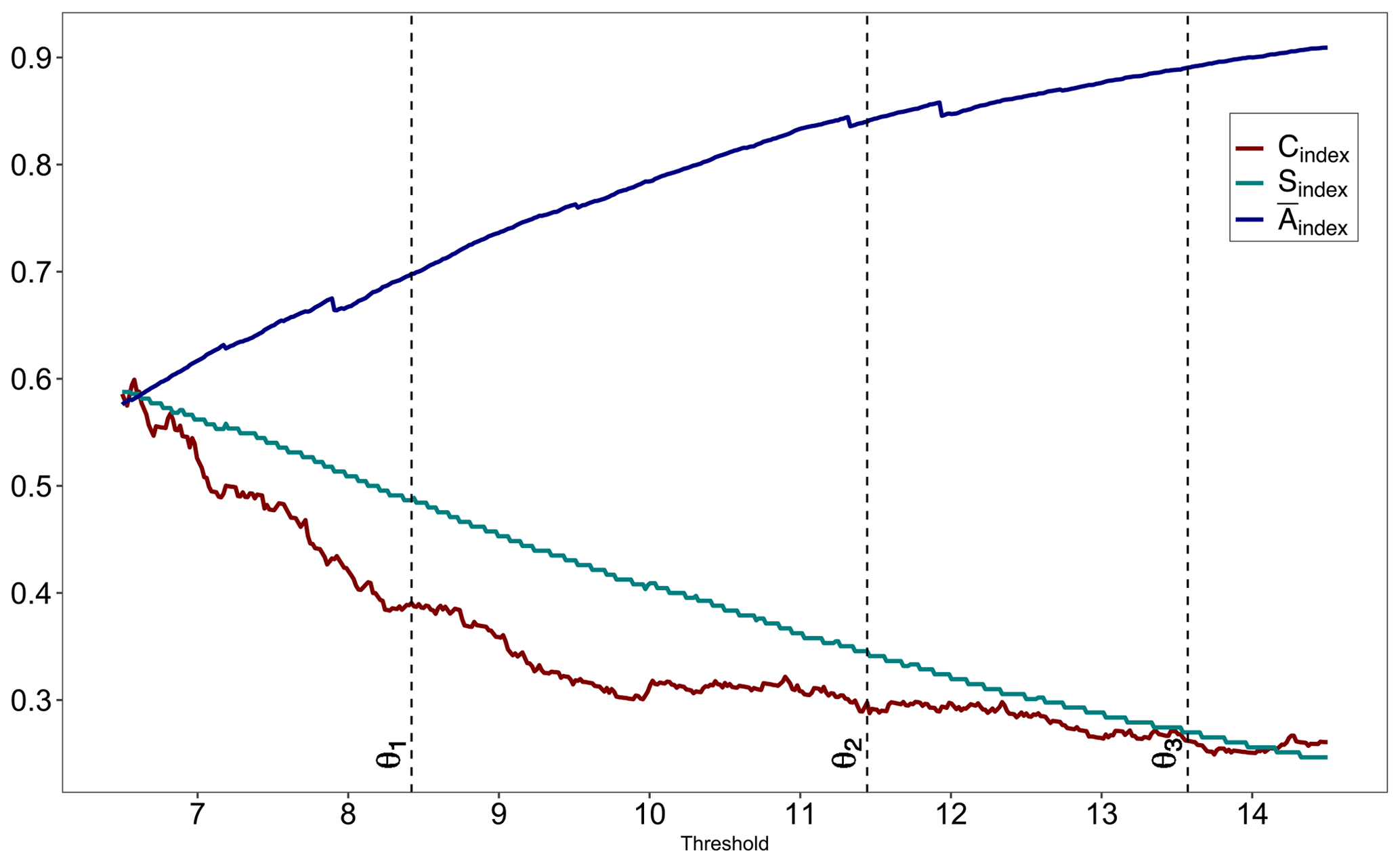
Figure 2 Geometric indices' evolution as a function of threshold for summer EFQ (GHCN-Daily dataset) with representative thresholds from low (θ₁), intermediate (θ₂), and high (θ₃) threshold clusters.

4.4 Time series clustering

Clustering is a statistical process applied in machine learning to group unlabeled data into homogeneous segments or clusters. The clusters are formed through segmentation of the data to maximize both inter-group dissimilarity and intra-group similarity according to objective criteria. The segmentation process entirely depends on a distance or dissimilarity metric, which measures how far away two objects are from each other. The degree of dissimilarity (or similarity) between the clustered objects is of significant importance in cluster analysis. Common dissimilarity metrics such as Euclidean and Manhattan are not suitable for time series clustering because they ignore serial correlations within the time series. Our main aim is to investigate the topological features of sequences of the conditional frequency images represented by multivariate series of geometric properties. These series may exhibit high degrees of serial correlation at different lag times (Fig. 2). Therefore, the first fundamental task in applying a clustering method is the selection of a dissimilarity metric that can capture these subtle characteristics. In particular, we are interested in discovering clusters of multivariate series of geometric properties with similar profiles representing large-scale extreme spatial patterns that can be buried under noise. For this purpose, several authors have suggested using dissimilarity measures based on the estimated autocorrelation functions of the time series (e.g., Galeano and Peña, 2000; Caiado et al., 2006). Here, we apply this approach to the multivariate series of geometric properties defined in the following way. Given f(s;θ) mapping to G_α[f(s;θ)], where $\mathit{\alpha }=[\mathrm{1},\mathrm{\dots },\mathrm{4}]$, we can alternatively map f(s;θ) to G_β[f(s;θ)], where $\mathit{\beta }=[\mathrm{1},\mathrm{\dots },\mathrm{4}]$. We let G_α[f(s;θ)] and G_β[f(s;θ)] be two geometric properties series, that is, $G_{\mathit{\alpha }}\left[f\right(\mathit{s};\mathit{\theta }\left)\right]=G_{\mathit{\alpha }}\left[f\right(\mathit{s};{\mathit{\theta }}_{\mathrm{1}}\left)\right],\mathrm{\dots },G_{\mathit{\alpha }}\left[f\right(\mathit{s};{\mathit{\theta }}_n\left)\right]$ and $G_{\mathit{\beta }}\left[f\right(\mathit{s};\mathit{\theta }\left)\right]=G_{\mathit{\beta }}\left[f\right(\mathit{s};{\mathit{\theta }}_{\mathrm{1}}\left)\right],\mathrm{\dots },G_{\mathit{\beta }}\left[f\right(\mathit{s};{\mathit{\theta }}_n\left)\right]$ for α≠β. We denote the vectors of the estimated autocorrelation coefficients of the geometric properties series G_α and G_β by ${\widehat{\mathit{\rho }}}_{G_{\mathit{\alpha }}}=\left({\widehat{\mathit{\rho }}}_{\mathrm{1},G_{\mathit{\alpha }}}\mathrm{\dots }{\widehat{\mathit{\rho }}}_{R,G_{\mathit{\alpha }}}\right)$ and ${\widehat{\mathit{\rho }}}_{G_{\mathit{\beta }}}=\left({\widehat{\mathit{\rho }}}_{\mathrm{1},G_{\mathit{\beta }}}\mathrm{\dots }{\widehat{\mathit{\rho }}}_{R,G_{\mathit{\beta }}}\right)$ for some R such as ${\widehat{\mathit{\rho }}}_{i,G_{\mathit{\alpha }}}\approx \mathrm{0}$ and ${\widehat{\mathit{\rho }}}_{i,G_{\mathit{\beta }}}\approx \mathrm{0}$ for i>R. Dissimilarity between G_α and G_β is measured by the following Euclidean distance:

$$\begin{array}{}\text{(6)}& d_{\text{ACF}}(G_{\mathit{\alpha }},G_{\mathit{\beta }})=\sqrt{\sum _{i=\mathrm{1}}^R({\widehat{\mathit{\rho }}}_{i,G_{\mathit{\alpha }}}-{\widehat{\mathit{\rho }}}_{i,G_{\mathit{\beta }}}{)}^{\mathrm{2}}}.\end{array}$$

Analogously, we define ${\widehat{\mathit{\varphi }}}_{ii,G_{\mathit{\alpha }}}$ and ${\widehat{\mathit{\varphi }}}_{ii,G_{\mathit{\beta }}}$ as the vectors of the estimated partial autocorrelation coefficients of G_α and G_β. A corresponding dissimilarity metric is given by

$$\begin{array}{}\text{(7)}& d_{\text{PACF}}(G_{\mathit{\alpha }},G_{\mathit{\beta }})=\sqrt{\sum _{i=\mathrm{1}}^R{\left({\widehat{\mathit{\varphi }}}_{ii,G_{\mathit{\alpha }}}-{\widehat{\mathit{\varphi }}}_{ii,G_{\mathit{\beta }}}\right)}^{\mathrm{2}}}.\end{array}$$

In the seasonal analysis that follows, the d_ACF and d_PACF measures vary between 0 and 0.001, indicating further how delicate the autocorrelation differences between geometric properties series can be. To calculate both distances, we used R package TSclust (Montero and Vilar, 2014).

The choice of the number of clusters K to form is another important task in the clustering algorithm. It typically involves iteratively searching for the number of clusters that optimizes a variety of criterion measures. Generally, cluster selection is still an unresolved problem requiring multiple iterations. However, in our case, it is somewhat simpler.

Previously we described that a balance between bias and variance was necessary when determining a threshold in EVT. A threshold choice for extremes in digital topology is also a challenge. A prudent question to pose is “what are desirable geometrical properties of the conditional frequency of extreme EFQ?” While it is difficult to generalize the shape and complexity indices, we postulate that choosing a threshold value with the desirable geometrical properties is an interplay between the connectivity index and area of non-zero points (referred to henceforth as connectivity/area trade-off). In cases involving both relatively low and very high threshold values connectivity index is close to one (see Eq. 3). The higher the threshold value, the lower the probability of simultaneous extreme events at two different spatial locations, the smaller the area of non-zero grid points. To balance this trade-off, we need to find a threshold value that is high enough to be practical to determine large-scale spatial patterns but not too high to cause the connectivity index to get close to one and the area of the non-zero pixels to be close to zero. Thus, there are three clusters of interest: the first cluster has multivariate series of geometric properties linked to the thresholds that are still high but may not be high enough to provide the desired geometric properties for the conditional frequency of extreme EFQ; the second cluster provides the high thresholds linked to desirable geometric properties; the third cluster produces the thresholds that are too high and impractical for our purpose. Therefore, we can observe that, if we have chosen more than three clusters, our task to deal with connectivity/area trade-off becomes very daunting. That is why we decided to concentrate our analysis on the second cluster to minimize potential connectivity/area impacts.

After selecting the dissimilarity measures and the number of clusters, it is necessary to select a clustering algorithm. The most popular partitioning clustering approaches are k-means and partitioning around medoids (PAM) (Kaufman and Rousseeuw, 1987). K-means creates cluster centers by averaging points within the cluster. However, this averaging process can be sensitive to outliers, and it also breaks the max-stability property, so that the mean of two maxima is no longer a maximum, which is an essential assumption in EVT. We, therefore, chose PAM, implemented in the cluster package in R (Maechler et al., 2017), which provides a more robust outcome, where each cluster is identified by its most representative object, called a medoid. Additionally, PAM preserves observational features of the dataset, which is essential for clustering extremes. The algorithm has two phases, BUILD and SWAP.

1. In the first phase, k representative objects are selected to form an initial clustering set.

2. In the second phase, an attempt is made to improve clustering by exchanging selected and unselected objects.

The objective of PAM is for all selected clusters to minimize average dissimilarity between their centrally located representative object and any other object in the same cluster. Further details can be found in Kaufman and Rousseeuw (1990). The quality of the resulting clusters and the choice of the number of clusters can be assessed using the “silhouette coefficient” (Rousseeuw, 1987), a statistic to determine how similar an object is to its own cluster (cohesion) compared to other clusters (separation). For an object i it is defined as follows:

$$\begin{array}{}\text{(8)}& \mathrm{Sil}\left(i\right)={\displaystyle \frac{b\left(i\right)-a\left(i\right)}{max\mathit{\left\{}a\right(i),b(i\left)\mathit{\right\}}}},\end{array}$$

where a(i) is the average dissimilarity of the object i to all other objects in its cluster and b(i) is the minimum average distance of object i to all other objects in the given cluster not containing i. The value of the silhouette coefficient Sil(i) ranges between −1 and 1, where a negative value is undesirable. If Sil(i)≈1, a strong structure has been found, which means that inter-cluster distance is much larger than intra-cluster distance. Conversely, if Sil(i)<0.25, no substantial structure has been found. The average silhouette coefficient $\stackrel{\mathrm{‾}}{\mathrm{Sil}}\left(K\right)$ can be used to evaluate the quality of segregation into K clusters, such as, for any finite K find $\underset{K}{max}\stackrel{\mathrm{‾}}{\mathrm{Sil}}\left(K\right)$.

4.5 Spatio-temporal threshold selection

Threshold selection is commonly used in the process of image segmentation (e.g., Sezgin and Sankur, 2004; Sahoo et al., 1988), that is, the process of using thresholds to partition an image into meaningful regions. This may include computer vision tasks such as finding a single threshold to separate an object in an image from its corresponding background, or separation of light and dark regions. However, these methods are not informative about spatial patterns (Kaur and Kaur, 2014) and are thus not appropriate for complex images (i.e., color images where multiband thresholding may be necessary) (Yogamangalam and Karthikeyan, 2013) such as those involved in this study. The problems we aim to solve involve identifying distinct extreme episodes that spread out over a large spatial domain and thus require more sophisticated methods.

Our threshold choice is directly linked to the outcome of the time series clustering step. The clustering solution produces results for the three clusters and their medoids, where every member is associated with the threshold and corresponding values of geometric properties series. As mentioned in the previous section, we address connectivity/area trade-off by selecting members from the second cluster only. The threshold selection is implemented as follows. First, we select maximum average silhouette coefficient between ${\stackrel{\mathrm{‾}}{\mathrm{Sil}}}_{\text{ACF}}$ and ${\stackrel{\mathrm{‾}}{\mathrm{Sil}}}_{\text{PACF}}$ and called it ${\stackrel{\mathrm{‾}}{\mathrm{Sil}}}_{\text{best}}$. This is necessary to select the best clustering solution between two distance measures. Next, the medoid from the second cluster is matched by the ${\stackrel{\mathrm{‾}}{\mathrm{Sil}}}_{\text{best}}$ to correspond to our threshold choice. Finally, the medoid index in the multivariate series of geometric properties is used to determine the corresponding geometric attributes. Equipped with both the high spatio-temporal threshold value and the spatial domain snapshot represented by geometric properties series, the user can make a more informative choice on a threshold appropriate for the particular class of extreme events and the needed applications.

4.6 Comparative analysis

To better understand the difference in spatial patterns produced by the two threshold selection methodologies, we compare geometrical properties between the STTC and CLST methods. The former is represented by a binary image of f(s;θ) conditioned on the fields' being a PEF, whereas the latter is a binary image of the usual location-specific frequency. However, in this form, the two frequencies are not compatible over space because they represent different subsets of the temporal domain. To put them on an equal footing, we start with a definition of a location-specific frequency. Let Y(s,t_j) be a spatio-temporal EFQ such that $\mathbf{Y}(\mathit{s},t_j)>\mathrm{0}$ for any $j=[\mathrm{1},\mathrm{\dots },M]$, M⩽T (i.e., our interest lies in “wet” EFQs in this comparative study). Then for any spatial pixel s∈𝒟, we can write

$$\begin{array}{}\text{(9)}& f_{\mathit{\tau }}\left(\mathit{s}\right)={\displaystyle \frac{\sum _{j=\mathrm{1}}^M{\text{𝟙}}_{\mathit{\left\{}\mathbf{Y}\right(\mathit{s},t_j)>\mathit{\lambda }[\mathbf{Y}(\mathit{s},t_j)\left]\mathit{\right\}}}}{M}},\end{array}$$

where λ[⋅] is the temporal quantile defined in Table 2 such as λ[Y(s,t_j)] = Y_τ(s) with τ=0.95. Note that f_τ(s) is a single spatial field representing the frequency of exceeding the τth quantile at each spatial location.

By its definition, the binary area calculated for all spatial pixels s and derived from A_index for this quantity will have more non-zero pixels than the segmented area of f(s;θ) and therefore will still not be adequate for the comparison. To reach a compromise, we threshold the spatial field for f_τ(s) to get as close to the area of f(s;θ) as possible. We can write this area-matched indicator as $f_{\mathit{\tau }}(\mathit{s};{\mathit{\theta }}^{\prime })$ for some threshold θ^′. Mathematically, we are searching for threshold θ^′ such that $A\left[f_{\mathit{\tau }}\right(\mathit{s};{\mathit{\theta }}^{\prime }\left)\right]\approx A\left[f\right(\mathit{s};\mathit{\theta }\left)\right]$. Henceforth, geometrical properties comparison is performed between $f_{\mathit{\tau }}(\mathit{s};{\mathit{\theta }}^{\prime })$ and the algorithmically determined f(s;θ).

5 Results

We apply the STTC algorithm to the EFQ of daily precipitation over the CONUS. Throughout, our analysis describes the spatial pattern and temporal evolution of the conditional frequency of an extreme, short-duration (i.e., daily), EFQ based on a high threshold. That is, our goal is to select a high threshold θ_h for the frequency of extreme EFQ conditioned on the fields' being a PEF based on daily precipitation rates. Based on empirical tests not shown here, we set η=0.99 for the univariate time series g_t and apply the temporal quantile definition for the function λ[⋅] from Table 2 with τ=0.95.

Heavy rainfall is seasonally dependent and varies in space and time. Thus, to understand the complete evolution of f(s;θ) and its spatial extent, we stratify the dataset by seasons defined as winter (DJF), spring (MAM), summer (JJA), and fall (SON). For every season, the clustering algorithm determines a high threshold value using the multivariate series of the geometric properties clustering procedure. Each cluster strength is represented via its average silhouette coefficient; values near one suggest strong clustering structures. Every threshold value is mapped to the corresponding set of geometric properties series, revealing the geometrical properties of the spatial image.

We demonstrate the performance of the STTC algorithm using inter-cluster comparison and determine important graphical properties of the three clusters. Also, we compare the results of our algorithm to the area-matched frequency (see Eq. 9) and identify the key differences between these two methods.

5.1 Inter-cluster comparison

To evaluate the performance of the clustering algorithm and the resultant geometrical properties of the conditional frequency of extreme EFQ, we characterize the results in the following manner.

• Cluster 1.

  Low thresholds. Expected both high values for the connectivity index and the area of non-zero points. The probability of simultaneous extreme events at two different spatial locations is relatively high.

• Cluster 2.

  Intermediate thresholds. Expected intermediate values (i.e., between the first and third clusters) for the area of non-zero points. The connectivity index is greater than zero and less than one-half. The threshold values from this cluster can be potentially used for modeling in EVT in conjunction with other statistical diagnostic tools. The probability of simultaneous extreme events at two different spatial locations is decreasing.

• Cluster 3.

  High thresholds. Expected small values for the area of non-zero points. The connectivity index is greater than zero. The probability of simultaneous extreme events at two different spatial locations is relatively low.

Tables 3–5 display the outcome of this process. Not surprisingly, the first low thresholds cluster has a higher connectivity and shape index and a larger areal extent and smaller complexity than the other two clusters. The average silhouette coefficient for this cluster is between 0.70 and 0.80. This cluster is useful if it is necessary to sample lower threshold values than the other two clusters. However, as we pointed out earlier, it may not be appropriate for extreme value analysis. As expected, the third high thresholds cluster has the lowest values for the connectivity and shape index and the smallest non-zero area among all other clusters. The average silhouette coefficient for the third cluster varies between 0.58 and 0.65. Finally, the second intermediate thresholds cluster has values of the geometric indices and the non-zero area between the first and second clusters. In addition, further examination of Fig. 2 reveals that the location of the second cluster falls within a low volatility regime for connectivity index, which is desirable for extreme value analysis as it helps to deal with connectivity/area trade-off. However, compared with the other two clusters, it results in a lower a(i) (i.e., the average dissimilarity of the object i to all other objects in its cluster) from Eq. (8) and, consequently, a lower average silhouette coefficient, which fluctuates between 0.46 and 0.50. However, it is still relatively high, as in all other clusters (i.e., above 0.25). Clearly, our clustering process characterizes the common features of multivariate series of geometric properties for the three clusters reasonably well. Hence, selecting a threshold from a different cluster for the conditional frequency of extreme EFQ can lead to different spatial forecast verification outcomes and ultimately to different statistical inferences regarding factors that explain extreme weather and climate events.

Table 3 Results of the Spatio-Temporal Threshold Clustering algorithm for the first (low thresholds) cluster.

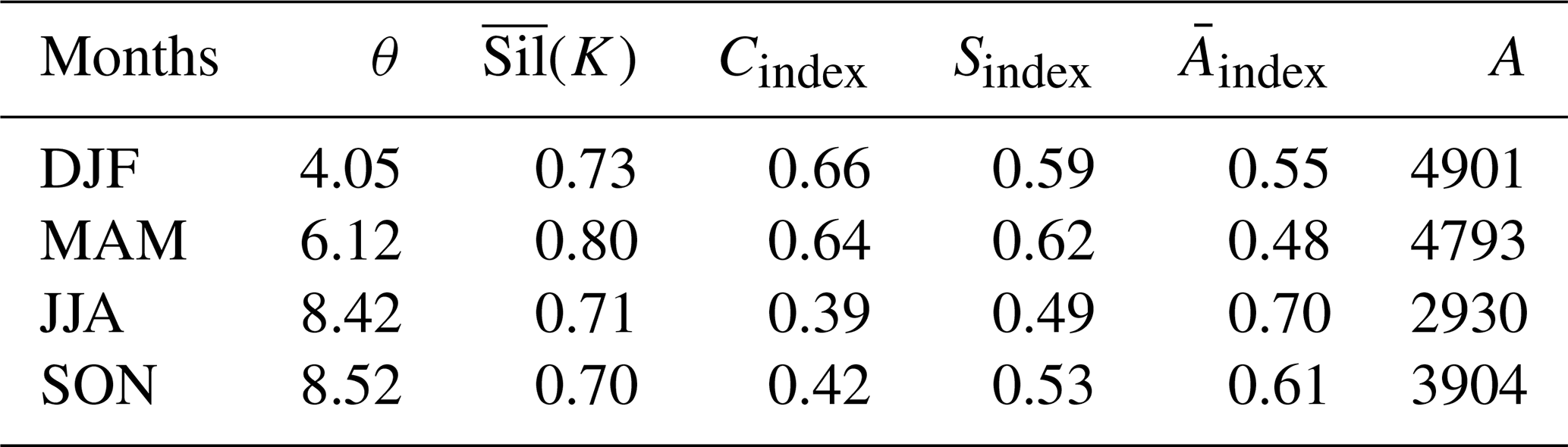
Table 4 Results of the Spatio-Temporal Threshold Clustering algorithm for the second (intermediate thresholds) cluster.

Table 5 Results of the Spatio-Temporal Threshold Clustering algorithm for the third (high thresholds) cluster.

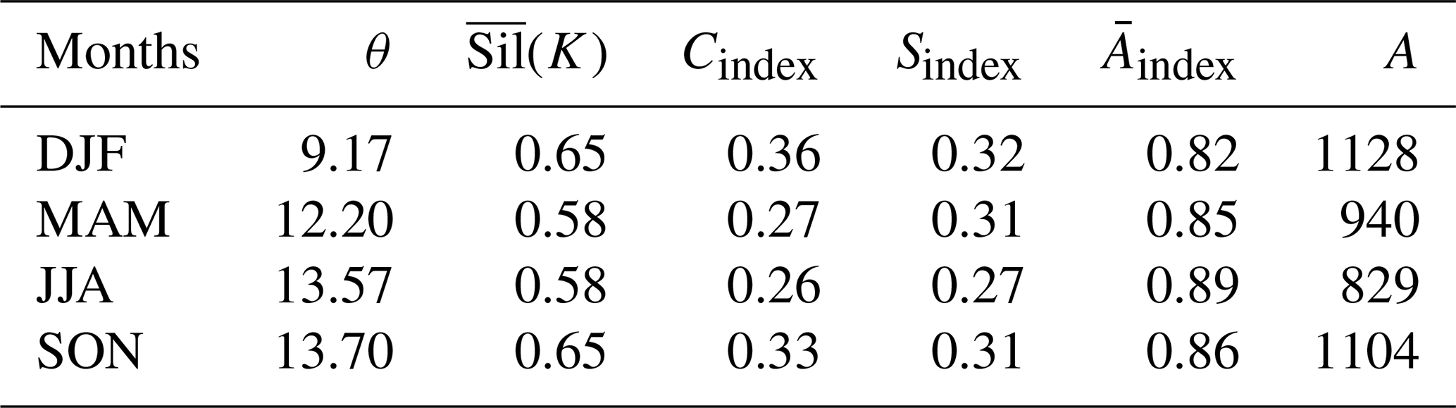
Figure 3 provides a graphical representation of the above results. The intermediate thresholds cluster has fewer isolated and more contiguous clusters (i.e., higher connectivity index), which are approximately circular in shape (i.e., higher shape index) and less scattered (i.e., lower complexity index). It occupies a broader spatial domain than the high thresholds cluster. The main advantage of having higher connectivity and larger areal extent attributes in spatial forecast verification for extremes is that it provides a more coherent representation of extremes patterns in space and, as a result, allows for a more informed decision about the causes, severity, and impact of the extremes under climate change, assuming climate models can simulate these graphical configurations reasonably well. These graphical qualities make the intermediate thresholds cluster the most likely choice for high threshold selection for the conditional frequency of extreme EFQ.

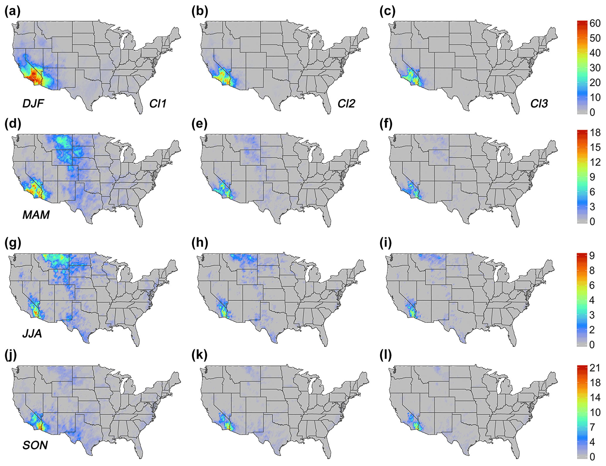
Figure 3 Frequency of extreme daily EFQ conditioned on the fields' being a PEF (GHCN-Daily dataset) for the three clusters: low thresholds cluster with threshold values from Table 3 (Cl1); intermediate thresholds cluster with threshold values from Table 4 (Cl2); high thresholds cluster with threshold values from Table 5 (Cl3), for every season: (a–c) winter (DJF); (d–f) spring; (g–i) summer; and (j–l) fall. All frequencies are stated in percent form.

The threshold selection methodology adopted here for f(s;θ) illustrates a fundamental difference with other conventional approaches for defining extreme event frequency. It is a common practice for threshold choice in univariate EVT to carry out an exploratory analysis or stability assessment of estimated parameters in the temporal domain without considering any spatial dependency. In our case, the threshold selection process has been conditioned on the fields' being a PEF, which allows analysis of temporal processes within a reasonably large spatial field, notwithstanding that many of the individual grid cells may not be necessarily extreme.

5.2 Comparison with the conventional approach

We stratify our dataset annually and by seasons, and Table 6 contains a summary of the large differences for connectivity, shape, and complexity indices between $f_{\mathit{\tau }}(\mathit{s};{\mathit{\theta }}^{\prime })$ and f(s;θ). Based on the experimental analysis (not shown here), we define a large difference for connectivity and shape indices as a difference smaller than −0.2, and for the complexity index the corresponding large difference is defined as greater than 0.2. In the table, we count those differences, and the resulting sum is divided by the number of samples (56 in our case). Analysis of the table clearly reveals that the smallest differences between $f_{\mathit{\tau }}(\mathit{s};{\mathit{\theta }}^{\prime })$ and f(s;θ) are observed in complexity and shape indices. This is because $f_{\mathit{\tau }}(\mathit{s};{\mathit{\theta }}^{\prime })$ is designed to closely match the area of f(s;θ). The ${\overline{A}}_{\text{index}}$ is related to the area in A_index, and the S_index is related to the square root of the area in P_min. On the other hand, it is apparent that the largest differences are confined to the connectivity index. That is, the algorithmically determined f(s;θ) has more connected and contiguous regions than the area-matched $f_{\mathit{\tau }}(\mathit{s};{\mathit{\theta }}^{\prime })$. To show this information graphically, we select a representative example with a large connectivity index difference equal to −0.27. Figure 4a and b display results for f(s;θ) and $f_{\mathit{\tau }}(\mathit{s};{\mathit{\theta }}^{\prime })$ respectively.

Table 6 Percent difference in geometric properties series between $f_{\mathit{\tau }}(\mathit{s};{\mathit{\theta }}^{\prime })$ and f(s;θ) when the difference is large.

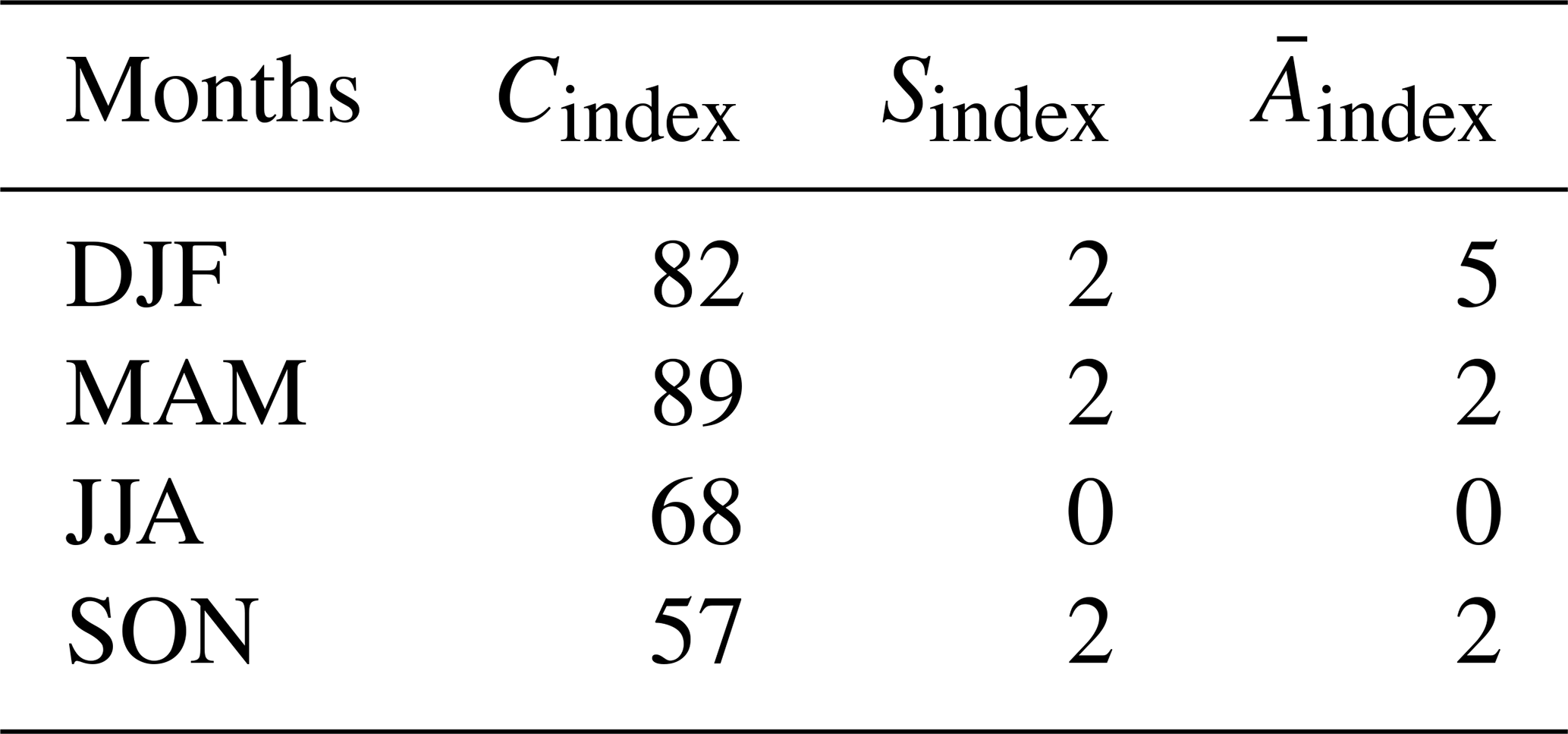
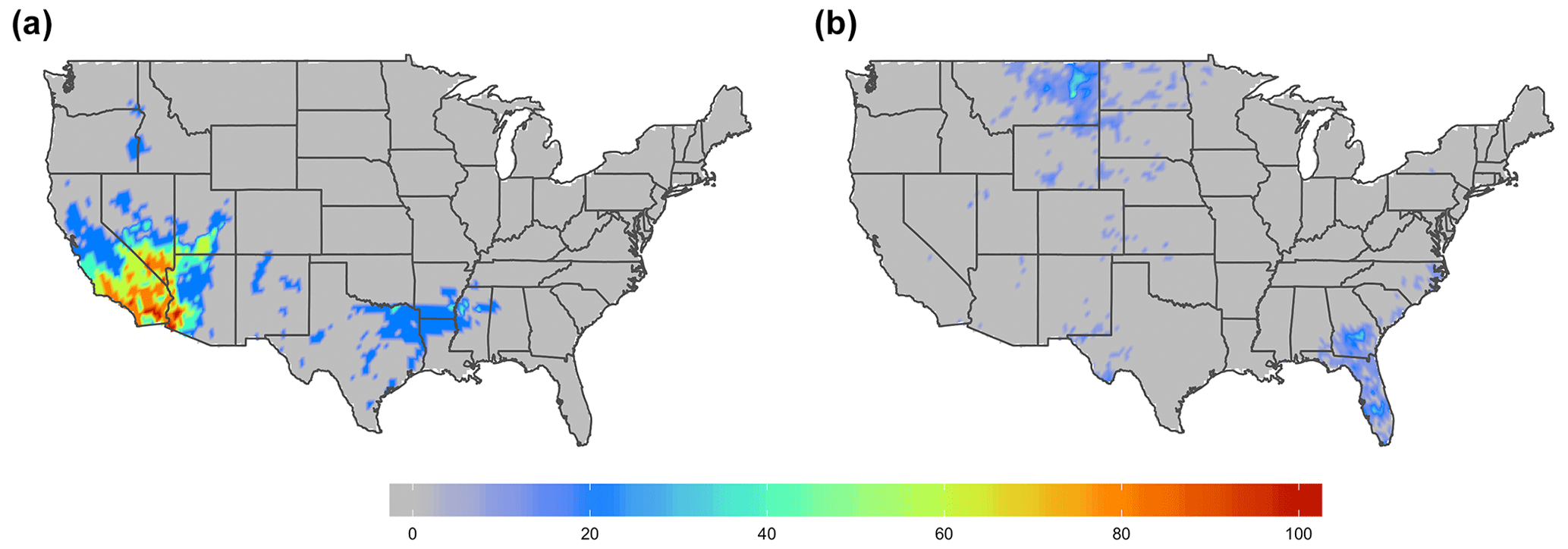
Figure 4 Examples of (a) f(s;θ) and (b) $f_{\mathit{\tau }}(\mathit{s};{\mathit{\theta }}^{\prime })$ for the winter of 2001 when the difference in $C_{\text{index}}=-$0.27, $S_{\text{index}}=-$0.12 and ${\overline{A}}_{\text{index}}=\mathrm{0}$.1 between $f_{\mathit{\tau }}(\mathit{s};{\mathit{\theta }}^{\prime })$ and f(s;θ). All frequencies are stated in percent form.

It is clear that the STTC algorithm has captured real spatial relationships by having low complexity and a greater number of contiguous (though a few were isolated), approximately circular-in-shape clusters. One of these regions covers most of the California, southern Nevada, Utah, and western Arizona, while another one starts in eastern Texas and stretches northeast along the Mississippi and Ohio rivers (see Fig. 4a). By comparison, the CLST method may or may not pick up important synoptic systems because it displays spatial fields with high complexity, including more isolated and disconnected clusters. For example, there are spatial areas with large $f_{\mathit{\tau }}(\mathit{s};{\mathit{\theta }}^{\prime })$ located in northeastern Montana, southern Georgia, and central Florida (see Fig. 4b).

To understand why f(s;θ) and $f_{\mathit{\tau }}(\mathit{s};{\mathit{\theta }}^{\prime })$ spatial representations have such different graphical properties, we consider the individual extreme event cases that we use to calculate these two frequencies. In the case of f(s;θ), we map these cases (Fig. 5; see caption) to the extreme weather episodes described in National Weather Service and local weather station reports. Figure 5a and b show high PEF values in southern–central California from the substantial rainfall and considerable snow accumulation in the mountains. Two significant snowstorms in California are displayed in Fig. 5c and d. Severe storms that spawn at least one tornado, causing ample rainfall and flooding in northeastern Texas and Arkansas, are shown in Fig. 5e. Conversely, since $f_{\mathit{\tau }}(\mathit{s};{\mathit{\theta }}^{\prime })$ calculations are done for every grid cell, we present a frequency distribution of the extreme cases in Fig. 5f. For every calendar day of the studied period from 1 January to 31 December 2001, we assign corresponding sequential number from 1 to 90. We display this number on the x axis. On the y axis, we show a frequency distribution of only extreme days that we use in $f_{\mathit{\tau }}(\mathit{s};{\mathit{\theta }}^{\prime })$ calculation (Eq. 9) across the entire spatial domain. High-frequency values imply a large contribution to $f_{\mathit{\tau }}(\mathit{s};{\mathit{\theta }}^{\prime })$ over s, whereas low values imply a small contribution. The red crosses mark days for the extreme cases from f(s;θ) calculation (Eq. 1). While the same days for the extreme cases appear in both frequencies, there were many other local extreme events present in $f_{\mathit{\tau }}(\mathit{s};{\mathit{\theta }}^{\prime })$ that were eliminated from f(s;θ) during the dimension reduction step. This explains why f(s;θ) and $f_{\mathit{\tau }}(\mathit{s};{\mathit{\theta }}^{\prime })$ have such different spatial representations in Fig. 4.

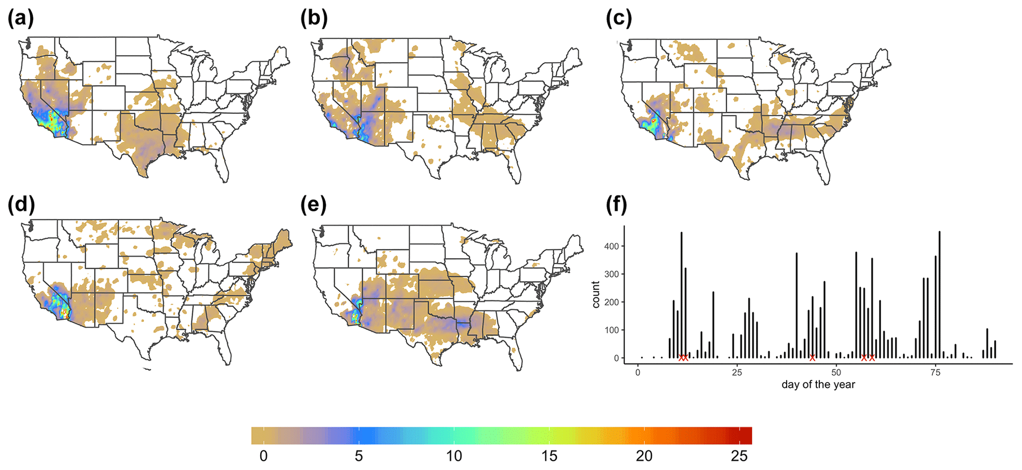
Figure 5 PEFs for individual extreme event cases that we use to calculate f(s;θ) from Fig. 4a: (a) 11 January 2001, (b) 12 January 2001, (c) 13 February 2001, (d) 26 February 2001, (e) 28 February 2001. PEF has no units. (f) Frequency distribution of only extreme days that we use in $f_{\mathit{\tau }}(\mathit{s};{\mathit{\theta }}^{\prime })$ calculation (Eq. 9) in Fig. 4b across the entire spatial domain. The red crosses mark days for the extreme cases from f(s;θ) calculation (Eq. 1).

Overall, while helpful for a location-specific analysis, the CLST method displays extremes at every non-empty grid cell and, in most cases, is deficient in geometric inter-connectivity between spatial pixels. At the same time, it has similar shape and complexity indices to the STTC algorithm. These graphical properties highlight the main advantage of the methodology adopted here – it represents larger-scale weather patterns such as storms and high- or low-pressure systems more accurately than the CLST method, by removing noisy data in both space and time, which is clearly desirable for spatial forecast verification of extreme events.

Figure 6 Annual linear trend for C_index of f(s;θ) from 1961 to 2016. Arrows show selected years, where n is the number of isolated structures and m is the number of non-zero grid cells (see Eq. 3). List of the years: (a) 1963, (b) 1970, (c) 1988, (d) 1998, (e) 2004; (f) 2014. All frequencies are stated in percent form.

6 Conclusions and applications

The lack of a universal definition of the concept “extreme” makes it difficult to compare different scientific studies of extreme events. It also makes statistical inference much harder and obfuscates transparency and risk management processes. The current work was an attempt to formalize this important concept. We introduced a new generalized Spatio-Temporal Threshold Clustering method (STTC) for extreme events using an integrative modeling approach framework. Step by step, we described the interworking of an algorithm that is applicable to a wide variety of essential field quantities (EFQs). We used EFQ constructed from gridded GHCN-Daily dataset comprised of 8516 stations from 1961 to 2016 across the CONUS. We applied a quantile-based dimension reduction methodology in space and time to identify extreme patterns for rainfall and droughts (Fig. 1). These precipitation patterns can be asymmetric for some storms due to the wind shear and are thus not fully detectable using conventional location-specific methods. To overcome this, we evaluated an entire spatial field comprised of relatively large-scale extreme patterns regardless of whether individual grid cells in space were extreme or not. Conditioned on these extreme patterns, the STTC method for the frequency of extreme EFQ allowed us to study not only individual local extreme episodes, but also the inter-connectivity, shape, complexity, and spatial extent of multiple extremes.

The threshold selection process, which is necessary for the conditional frequency calculation, was based on a multivariate series of geometric properties clustering analysis. We used a silhouette coefficient to measure a quality of resulting clusters. In Tibshirani et al. (2001) a variety of other metrics were used to decide on the number of clusters for non-extreme events, and it was found that the silhouette method did not have the best performance. However, in our case, we performed clustering of the multivariate series of geometric properties for the extreme events, and we predetermined the number of clusters and set them to three.

We analyzed the output of the clustering algorithm and we demonstrated that the intermediate thresholds cluster was the most suitable choice to deal with connectivity/area trade-off for analysis of extreme events when compared to the low thresholds and high thresholds clusters. In addition, we established that the STTC algorithm had more spatial connectivity and, in most cases, similar complexity and shape when compared to the CLST method. This finding is particularly important for spatial forecast verification of high-resolution climate models.

Our new threshold selection algorithm has a number of potential benefits. It objectively automates the threshold selection process through the clustering algorithm and can ultimately be used in conjunction with spatial forecast verification and modeling of extreme events. It is adaptable to model extremes with both high and low threshold choices. It incorporates spatial and temporal dependence in one holistic modeling framework, thus opening an opportunity for future analysis of statistical inference of extreme events for univariate and possibly multivariate EFQ in space and time, which is not currently possible using conventional location-specific methods. It is less sensitive to the data grid size when performing areal mean interpolation (Chen and Knutson, 2008) and can thus provide a consistent spatial pattern across different grid resolutions. It also links the chosen threshold to desired geometrical properties, which offers users more informed and flexible choices in selecting extreme events. The algorithm is relatively fast for large datasets and could be embedded within climate modeling systems (global or regional) to identify synoptic-scale spatial patterns that are linked to the individual extreme episodes. However, it entails selecting a range of initial thresholds, which could be time-consuming for some users. The proposed threshold selection method requires spatially and temporally varying data and not applicable in modeling location-specific single extreme events (Cattiaux and Ribes, 2018). The algorithm is quite stable to small changes in the range of the initial thresholds necessary for time series clustering step. However, it is sensitive to the choice of λ[⋅] as well as to spatial and temporal quantile values, especially when the spatio-temporal data size is small. The user must decide what form of λ[⋅] is the most suitable for the underlying application and what quantile values are capturing essential extreme episodes for the specific domain of interest.

The algorithm can be used to compare biases between global and regional climate models (Liang et al., 2012) and possibly uncover the underlying physical mechanisms of these biases. Furthermore, an interesting perspective of this work is to determine whether or not one can capture dynamic and thermodynamic properties of the spatio-temporal structure of the conditional frequency of extreme EFQ from an ensemble of simulations in a single climate model with multiple physics configurations (Sun and Liang, 2020) or a set of different climate models (Min et al., 2011). Another potential application is to investigate how the observed spatio-temporal processes of the conditional frequency of extreme EFQ have changed and the causes of those changes, utilizing the most recent detection and attribution framework (e.g., Knutson et al., 2017; Ribes et al., 2017).

We foresee that our novel threshold selection approach could lead to new insights into spatial trends analysis in patterns of extreme EFQs. Figure 6 shows a linear downward trend for the connectivity index (C_index) of f(s;θ) from 1961 to 2016, where the conditional frequencies are objectively and independently derived for each year. The model fit (intercept $=\mathrm{5.57}\pm \mathrm{1.07},p\ll \mathrm{0.001}$; slope $=-\mathrm{0.003}\mp \mathrm{0.0005},p\ll \mathrm{0.001}$; R²=0.29) exhibited about the same variability between 1961 and 1988 (interquartile range ≈0.07) and between 1989 and 2016 (≈0.08). The downward trend in C_index is primarily caused by the upward trend (not shown here) in the parameter n (i.e., number of isolated structures). We found no trend in the parameter m (i.e., the number of non-zero grid cells) (see Eq. 3). Figure 6a–f display f(s;θ) for selective years with decreasing n and corresponding m values. To the untrained eye, it is difficult to see any periodic changes in the number of isolated structures. However, the supplied numerical values should substantiate our claim.

An important caveat of C_index is that it is a binary index. As such, it only calculates all components based on the number of non-zero grid cells in the spatial patterns by setting values below a threshold to zero and those above to one. It does not provide any information about the original raw intensities. However, evaluation of this index at different threshold values can provide some information about the error intensity (Gilleland, 2017b). The upward trend in the number of isolated structures implies that the distribution of conditional frequency of extreme precipitation is changing from large-scale well-connected spatial patterns to smaller-scale less contiguous rainfall clusters. In order to understand why we observe the distributional change, it is important to establish the linkages between changes in circulation and other essential climate variables (e.g., temperature and precipitation). If the trend continues, we expect to see more localized droughts and heat waves, especially during the summer months. It would also create a tremendous challenge for weather forecasting and climate adaptation efforts as the forecast skill drops significantly at smaller scales. Thus, the STTC offers a unique way of performing diagnostic analysis of the large-scale weather patterns specifically associated with these extreme episodes, and such analysis for the detected trend is in progress.

Appendix A