Forecast score distributions with imperfect observations

The field of statistics has become one of the mathematical foundations in forecast evaluation studies, especially with regard to computing scoring rules. The classical paradigm of scoring rules is to discriminate between two different forecasts by comparing them with observations. The probability distribution of the observed record is assumed to be perfect as a verification benchmark. In practice, however, observations are almost always tainted by errors and uncertainties. These may be due to homogenization problems, instrumental deficiencies, the need for indirect reconstructions from other sources (e.g., radar data), model errors in gridded products like reanalysis, or any other data-recording issues. If the yardstick used to compare forecasts is imprecise, one can wonder whether such types of errors may or may not have a strong influence on decisions based on classical scoring rules. We propose a new scoring rule scheme in the context of models that incorporate errors of the verification data. We rely on existing scoring rules and incorporate uncertainty and error of the verification data through a hidden variable and the conditional expectation of scores when they are viewed as a random variable. The proposed scoring framework is applied to standard setups, mainly an additive Gaussian noise model and a multiplicative Gamma noise model. These classical examples provide known and tractable conditional distributions and, consequently, allow us to interpret explicit expressions of our score. By considering scores to be random variables, one can access the entire range of their distribution. In particular, we illustrate that the commonly used mean score can be a misleading representative of the distribution when the latter is highly skewed or has heavy tails. In a simulation study, through the power of a statistical test, we demonstrate the ability of the newly proposed score to better discriminate between forecasts when verification data are subject to uncertainty compared with the scores used in practice. We apply the benefit of accounting for the uncertainty of the verification data in the scoring procedure on a dataset of surface wind speed from measurements and numerical model outputs. Finally, we open some discussions on the use of this proposed scoring framework for non-explicit conditional distributions.

1 Introduction

Probabilistic forecast evaluation generally involves the comparison of a probabilistic forecast cumulative distribution function (cdf) F (in the following, we assume that F admits a probability density function f) with verification data y that could be of diverse origins (Jolliffe and Stephenson, 2004; Gneiting et al., 2007). In this context verification data are, most of the time, but not exclusively, observational data. Questions related to the quality and variability of observational data have been raised and tackled in different scientific contexts. For instance, data assimilation requires careful estimation of uncertainties related to both numerical models and observations (Daley, 1993; Waller et al., 2014; Janjić et al., 2017). Apart from a few studies (see, e.g., Hamill and Juras, 2006; Ferro, 2017), error and uncertainty associated with the verification data have rarely been addressed in forecast evaluation. Nonetheless, errors in verification data can lead to severe mischaracterization of probabilistic forecasts, as illustrated in Fig. 1, where a perfect forecast (a forecast with the same distribution as the true data) appears underdispersed when the verification data have a larger variance than the true process. In the following, the underlying hidden process that is materialized by model simulations or measured through instruments will be referred to as the true process. Forecast evaluation can be performed qualitatively through visual inspection of statistics of the data such as in Fig. 1 (see, e.g., Bröcker and Ben Bouallègue, 2020) and quantitatively through the use of scalar functions called scores (Gneiting et al., 2007; Gneiting and Raftery, 2007). In this work, we focus on the latter, and we illustrate and propose a framework based on hidden variables to embed imperfect verification data in scoring functions via priors on the verification data and on the hidden state.

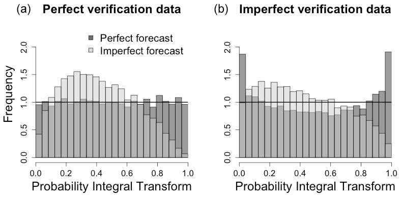
Figure 1 “Perfect” (dark grey) and “imperfect” (light grey) synthetic forecasts, with respective distributions 𝒩(0,2) and 𝒩(0.5,4), are compared with “perfect” verification data (a) with distribution 𝒩(0,2) and imperfect verification data Y and (b) with distribution 𝒩(0,3). Comparing a perfect forecast (forecast with the same distribution as the true data) to corrupted verification data leads to an apparent underdispersion of the perfect forecast.

1.1 Motivating example

To illustrate the proposed work, we consider surface wind data from a previous work (Bessac et al., 2018). Time series of ground measurements from the NOAA Automated Surface Observing System (ASOS) network are available at ftp://ftp.ncdc.noaa.gov/pub/data/asos-onemin, last access: 8 September 2021 and are extracted at 1 min resolution. We focus on January 2012 in this study; the data are filtered via a moving-average procedure and considered at an hourly level, leading to 744 data points. These ground-station data are considered verification data in the following. Outputs from numerical weather prediction (NWP) forecasts are generated by using WRF v3.6 (Skamarock et al., 2008), a state-of-the-art numerical weather prediction system designed to serve both operational forecasting and atmospheric research needs. The NWP forecasts are initialized by using the North American Regional Reanalysis fields dataset that covers the North American continent with a resolution of 10 min of a degree, 29 pressure levels (1000–100 hPa, excluding the surface), every 3 h from the year 1979 until the present. Simulations are started every day during January 2012 with a forecast lead time of 24 h and cover the continental United States on a grid of 25×25 km with a time resolution of 10 min. Only one trajectory is simulated in this study. As observed in Fig. 2, the uncertainty associated with observation data can affect the evaluation of the forecast. As an extension, if two forecasts were to fall within the uncertainty range of the observations, it would require a non-trivial choice from the forecaster to rank forecasts.

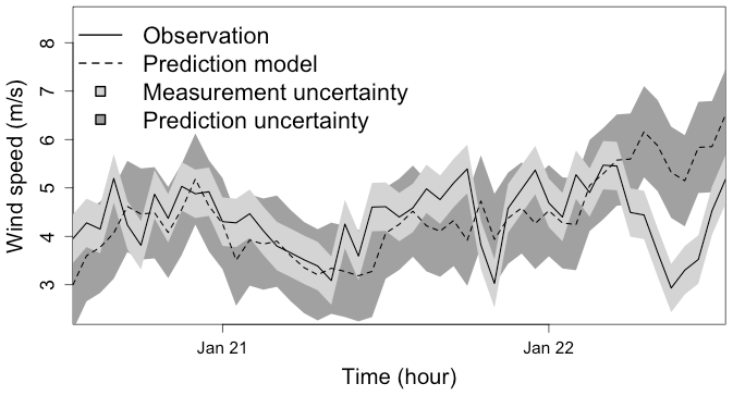
Figure 2 Time series of surface wind speed measurements of two days of January 2012 in Wisconsin, USA. The solid line represents ground measurements and the light grey shaded area represents observational uncertainty (±σ, with σ=0.5 defined in Pinson and Hagedorn, 2012). The dashed line represents a numerical model output and the model uncertainty in dark grey shade. The model uncertainty refers to the standard deviation computed on the available forecast time series.

We will apply our proposed scoring framework to this dataset in Sect. 5.2 and compute scores embedding this uncertainty.

1.2 Imperfect verification data and underlying physical state

In verification and recalibration of ensemble forecasts, an essential verification step is to find data that precisely identify the forecast events of interest, the so-called verification dataset (see, e.g., Jolliffe and Stephenson, 2004). Jolliffe and Stephenson (2004), in Sect. 1.3 of their book, discussed the uncertainty associated with verification data, such as sampling uncertainty, direct measurement uncertainty, or changes in locations in the verification dataset. Verification data arise from various sources and consequently present various types of errors and uncertainties, such as measurement error (Dirkson et al., 2019), design, and quality: e.g., gridded data versus weather stations, homogenization problems, sub-sampling variability (Mittermaier and Stephenson, 2015), or mismatching resolutions. Resolution mismatching is becoming an issue due to weather or regional climate models running at ever finer resolution with increased fidelity for which observational data are rarely available for evaluation, hence requiring us to account for up- or down-scaling error. In order to provide accurate forecast evaluations, it is crucial to distinguish and account for these types of errors. For instance, the effect of observational error can be stronger at a short-term horizon when forecast error is smaller. Additive models have been used for the observational error (Ciach and Krajewski, 1999; Saetra et al., 2004) or used to enhance coarser resolutions to allow comparison with fine-resolution data (Mittermaier and Stephenson, 2015). In the following, we will present an additive and a multiplicative framework based on a hidden variable to embed uncertainty in data sources.

A common way of modeling errors is by representing the truth as a hidden underlying process also called the state (Kalman, 1960; Kalman and Bucy, 1961). Subsequently each source of data is seen as a proxy of the hidden state and modeled as a function of it. This forms the basis of data assimilation models where the desired state of the atmosphere is estimated through the knowledge of physics-based models and observational data that are both seen as versions of the non-observed true physical state. In the following, we base our scoring framework on the decomposition of the verification data as a function of a hidden true state, referred to as X, and an error term.

1.3 Related literature

Uncertainty and errors arise from various sources, such as the forecast and/or the verification data (predictability quality, uncertainty, errors, dependence and correlation, time-varying distribution), and the computational approximation of scores. A distribution-based verification approach was initially proposed by Murphy and Winkler (1987), where joint distributions for forecast and observation account for the information and interaction of both datasets. Wilks (2010) studied the effect of serial correlation of forecasts and observations on the sampling distributions of Brier score and, in particular, serially correlated forecasts inflate its variance. Bolin and Wallin (2019) discussed the misleading use of average scores, in particular for the continuous ranked probability score (CRPS) that is shown to be scale-dependent, when forecasts have varying predictability such as in non-stationary cases or exhibit outliers. Bröcker and Smith (2007), in their conclusion, highlighted the need to generalize scores when verification data are uncertain in the context of properness and locality. More specifically, robustness and scale-invariance corrections of the CRPS are proposed to account for outliers and varying predictability in scoring schemes. Concerning the impact of the forecast density approximation from finite ensembles, Zamo and Naveau (2018) compared four CRPS estimators and highlighted recommendations in terms of the type of ensemble, whether random or a set of quantiles. In addition, several works focus on embedding verification data errors and uncertainties in scoring setups. Some methods aimed at correcting the verification data and using regular scoring metrics, such as perturbed ensemble methods (Anderson, 1996; Hamill, 2001; Bowler, 2008; Gorgas and Dorninger, 2012). Other works modeled observations as random variables and expressed scoring metrics in that context (Candille and Talagrand, 2008; Pappenberger et al., 2009; Pinson and Hagedorn, 2012). Some approaches directly modified the expression of metrics (Hamill and Juras, 2006; Ferro, 2017), and others (see, e.g., Hamill and Juras, 2006) accounted for varying climatology by sub-dividing the sample into stationary ones. In Ciach and Krajewski (1999) and Saetra et al. (2004), additive errors were embedded in scores via convolution. Analogously to the Brier score decomposition of Murphy (1973), Weijs and Van De Giesen (2011) and Weijs et al. (2010) decomposed the Kullback–Leibler divergence score and the cross-entropy score into uncertainty into reliability and resolution components in order to account for uncertain verification data. Kleen (2019) discussed score-scale sensitivity to additive measurement errors and proposed a measure of discrepancy between scores computed on uncorrupted and corrupted verification data.

1.4 Proposed scoring framework

The following paper proposes an idealized framework to express commonly used scores with observational uncertainty and errors. The new framework relies on the decomposition of the verification data y into a “true” hidden state x and an error term and on the representation of scores as a random variable when the verification data are seen as a random variable. Information about the hidden state and the verification data is embedded via priors in the scoring framework, sharing analogies with classical Bayesian analysis (Gelman et al., 2013). More precisely, the proposed framework relies on the knowledge about the conditional distribution of the “true” hidden state given the verification data or about information which allows us to calculate that conditional distribution.

Section 2 introduces a scoring framework that accounts for errors in the verification data for scores used in practice. Sections 3 and 4, respectively, implement the additive and multiplicative error-embedding cases for the logarithmic score (log score) and CRPS. Section 5 illustrates the merits of scores in a simulation context and in a real application case. Finally, Sect. 6 provides a final discussion and insights into future works. In particular, we discuss the possible generalization of the proposed scoring framework when the decomposition of the verification data y into a hidden state x and an error does not fall into an additive or multiplicative setting as in Sects. 3 and 4.

2 Scoring rules under uncertainty

In the following, we propose a version of scores based on the conditional expectation of what is defined as an “ideal” score given the verification data tainted by errors, when scores are viewed as random variables. The idea of conditional expectation was also used in Ferro (2017) but with a different conditioning and is discussed below as a comparison.

2.1 Scores as random variables

In order to build the proposed score version as well as to interpret scores further than through their mean and assess for their uncertainty, we will rely on scores represented as random variables. In practice, scores are averaged over all available verification data y, and the uncertainty associated with this averaged score is mostly neglected. However, this uncertainty is revealed to be significant, as pointed out in Dirkson et al. (2019), where confidence intervals were computed through bootstrapping. In order to assess the probability distribution of score s₀, we assume Y is a random variable representing the verification data y and write a score as a random variable s₀(F,Y), where F is the forecast cdf to be evaluated. This representation gives access to the score distribution and enables us to explore the uncertainty of the latter. A few works in the literature have already considered scores to be random variables and performed the associated analysis. In Diebold and Mariano (2002) and Jolliffe (2007), score distributions were considered to build confidence intervals and hypothesis testing to assess differences in score values when comparing forecasts to the climatology. In Wilks (2010), the effect of serial correlation on the sampling distributions of Brier scores was investigated. Pinson and Hagedorn (2012) illustrated and discussed score distributions across different prediction horizons and across different levels of observational noise.

2.2 Hidden state and scoring

Scores used in practice are evaluated on verification data y, s₀(F,y). We define the “ideal” score as s₀(F,x), where x is the realization of the hidden underlying “true” state that gives rise to the verification data y. Ideally, one would use x to provide the best assessment of forecast F quality through s₀(F,x); however, since x is not available, we consider the best approximation of s₀(F,x) given the observation y in terms of the L² norm via the conditional expectation. For a given score s₀, we propose the following score version $s_{\vee }(.,y)$:

$$\begin{array}{}\text{(1)}& s_{\vee }(F,y)=\mathbb{E}\left(s_{\mathrm{0}}(F,X)|Y=y\right),\end{array}$$

where X is the true hidden state, Y is the random variable representing the available observation used as verification data, and F is the forecast cdf to be evaluated. One can view this scoring framework incorporating information about the discrepancy between the true state and the verification data in terms of errors and uncertainty in a Bayesian setting. To compute Eq. (1), we assume that the distributional features of the law of X and the conditional law of [Y|X], where [.] and $[.|.]$ denote, respectively, marginal and conditional distributions, are directly available or can be obtained. This is the classical framework used in data assimilation when both observational and state equations are given, and the issue is to infer the realization x given observations y; see also our example in Sect. 5.2. Under this setup, the following properties hold for the score s_∨:

$$\begin{array}{}\text{(2)}& \begin{array}{rl}{\mathbb{E}}_X\left[s_{\mathrm{0}}(F,X)\right]& ={\mathbb{E}}_Y\left[s_{\vee }(F,Y)\right],\\ {\mathbb{V}}_X\left[s_{\mathrm{0}}(F,X)\right]& \ge {\mathbb{V}}_Y\left[s_{\vee }(F,Y)\right],\text{ for any forecast cdf}F.\end{array}\end{array}$$

Details of the computations are found in Appendix A. The first equality guarantees that any propriety attached to the mean value of s₀ is preserved with s_∨. The second inequality arises from the law of total variance and implies a reduced dispersion of the corrected score compared to the ideal score. This can be explained by the prior knowledge on the verification data that reduces uncertainty in the score. These properties are illustrated with simulated examples and real data in Sect. 5.

As a comparison, Ferro (2017) proposed a mathematical scheme to correct a score when error is present in the verification data y. Ferro's modified score, denoted s_F(f,y) in this work, is derived from a classical score, say s₀(f,x), where x is the hidden true state. With these notations, the corrected score s_F(f,y) is built such that it respects the following conditional expectation:

$$s_{\mathrm{0}}(f,x)=\mathbb{E}\left(s_F(f,Y)|X=x\right).$$

In other words, the score s_F(f,y) computed from the ys provides the same value on average as the proper score computed from the unobserved true state xs. The modified score s_F explicitly targets biases in the mean induced by imperfect verification data. In terms of assumptions, we note that the conditional law of Y given X needs to be known in order to compute s₀(f,x) from s_F(f,y); e.g., see Definitions 2 and 3 in Ferro (2017). In particular, in Ferro (2017) the correction framework is illustrated with the logarithmic score in the case of a Gaussian error model, i.e., $\left[Y\right|X=x]\sim \mathcal{N}(x,{\mathit{\omega }}^{\mathrm{2}})$.

Implementation and generalization

The proposed score reveals desirable mathematical properties of unbiasedness and variance reduction while accounting for the error in the verification data; however, it relies on the knowledge of [X|Y] or equivalently of [Y|X] and [X]. We assume that the decomposition of Y into a hidden state X and an error is given and is fixed with respect of the evaluation framework. Additionally, the new framework relies on the necessity to integrate s₀(f,x) against conditional distributions, which might require some quadrature approximations in practice when closed formulations are not available. In this work, we assume we have access to the climatology distribution, and we rely on this assumption to compute the distribution of X or priors of its distribution. However, depending on the context and as exemplified in Sect. 5.2, alternative definitions and computations of X can be considered, as for instance relying on known measurement error models. Nonetheless, as illustrated in Sects. 3 and 4, the simplifying key to the score derivation in Eq. (1) is to use Bayesian conjugacy when applicable. This is illustrated in the following sections with a Gaussian additive case and a Gamma multiplicative case. Although the Bayesian conjugacy is a simplifying assumption, as in most Bayesian settings it is not a necessary condition, and for cases with non-explicit conjugate priors, all Bayesian and/or assimilation tools (e.g., via sampling algorithms such as Markov chain Monte Carlo methods (Robert and Casella, 2013) or non-parametric approaches such as Dirichlet processes) could be used to draw samples from [X|Y] and estimate the distribution $\left[s_{\mathrm{0}}\right(F,X\left)\right|Y=y]$ for a given $s_{\mathrm{0}}(F,.)$. Finally, in the following we assume that distributions have known parameters; however, this assumption can be relaxed by considering prior distributions on each involved parameter via hierarchical Bayesian modeling. The scope of this paper is to provide a conceptual tool, and the question of parameter estimation, besides the example in Sect. 5, is not treated in detail. In Sect. 5, we apply the proposed score derivation to the aforementioned surface wind data example described in the introduction. In Sect. 6, we discuss the challenges of computing scores as defined in Eq. (1) or in Ferro (2017) in more general cases of state-space models that are not limited to additive or multiplicative cases.

3 Gaussian additive case

As discussed earlier, a commonly used setup in applications is when errors are additive and their natural companion distribution is Gaussian. Hereafter, we derive the score from Eq. (1) for the commonly used log score and CRPS in the Gaussian additive case, where the hidden state X and the verification data Y are linked through the following system:

$$\text{ Model (A)}\left\{\begin{array}{l}X\sim \mathcal{N}\left({\mathit{\mu }}_{\mathrm{0}},{\mathit{\sigma }}_{\mathrm{0}}^{\mathrm{2}}\right),\\ Y=X+\mathcal{N}\left(\mathrm{0},{\mathit{\omega }}^{\mathrm{2}}\right),\end{array}\right.$$

where Y is the observed verification data, X is the hidden true state, and all Gaussian variables are assumed to be independent. In the following, for simplicity we consider 𝔼(X)=𝔼(Y); however, one can update the model easily to mean-biased verification data Y. Parameters are supposed to be known from the applications; one could use priors on the parameters when estimates are not available. In the following, we express different versions of the log score and CRPS: the ideal version, the used-in-practice version, and the error-embedding version from Eq. (1). In this case, as well as in Sect. 4, since conditional distributions are expressed through Bayesian conjugacy, most computational efforts rely on integrating the scores against the conditional distributions.

3.1 Log-score versions

For a Gaussian predictive probability distribution function (pdf) f with mean μ and variance σ², the log score is defined by

$$\begin{array}{}\text{(3)}& s_{\mathrm{0}}(f,x)=\log \mathit{\sigma }+{\displaystyle \frac{\mathrm{1}}{\mathrm{2}{\mathit{\sigma }}^{\mathrm{2}}}}(x-\mathit{\mu }{)}^{\mathrm{2}}+{\displaystyle \frac{\mathrm{1}}{\mathrm{2}}}\log \mathrm{2}\mathit{\pi }\end{array}$$

and has been widely used in the literature. Ideally, one would access the true state X and evaluate forecast against its realizations x; however, since X is not accessible, scores are computed against observations y:

$$\begin{array}{}\text{(4)}& s_{\mathrm{0}}(f,y)=\log \mathit{\sigma }+{\displaystyle \frac{\mathrm{1}}{\mathrm{2}{\mathit{\sigma }}^{\mathrm{2}}}}(y-\mathit{\mu }{)}^{\mathrm{2}}+{\displaystyle \frac{\mathrm{1}}{\mathrm{2}}}\log \mathrm{2}\mathit{\pi }.\end{array}$$

Applying basic properties of Gaussian conditioning, our score defined by Eq. (1) can be written as

$$\begin{array}{}\text{(5)}& \begin{array}{rl}{s}_{\vee }(f,y)=& \log \mathit{\sigma }+{\displaystyle \frac{\mathrm{1}}{\mathrm{2}{\mathit{\sigma }}^{\mathrm{2}}}}\mathit{\{}{\displaystyle \frac{{\mathit{\omega }}^{\mathrm{2}}{\mathit{\sigma }}_{\mathrm{0}}^{\mathrm{2}}}{{\mathit{\sigma }}_{\mathrm{0}}^{\mathrm{2}}+{\mathit{\omega }}^{\mathrm{2}}}}\\ & +{\left(\stackrel{\mathrm{‾}}{y}-\mathit{\mu }\right)}^{\mathrm{2}}\mathit{\}}+{\displaystyle \frac{\mathrm{1}}{\mathrm{2}}}\log \mathrm{2}\mathit{\pi },\\ & \text{where }\stackrel{\mathrm{‾}}{y}={\displaystyle \frac{{\mathit{\omega }}^{\mathrm{2}}}{{\mathit{\sigma }}_{\mathrm{0}}^{\mathrm{2}}+{\mathit{\omega }}^{\mathrm{2}}}}{\mathit{\mu }}_{\mathrm{0}}+{\displaystyle \frac{{\mathit{\sigma }}_{\mathrm{0}}^{\mathrm{2}}}{{\mathit{\sigma }}_{\mathrm{0}}^{\mathrm{2}}+{\mathit{\omega }}^{\mathrm{2}}}}y.\end{array}\end{array}$$

In particular, $\stackrel{\mathrm{‾}}{y}=\mathbb{E}\left(X\right|Y=y)$ arises from the conditional expectation of $s_{\vee }(f,Y)$ in Eq. (3) and is a weighted sum that updates the prior information about $X\sim \mathcal{N}({\mathit{\mu }}_{\mathrm{0}},{\mathit{\sigma }}_{\mathrm{0}}^{\mathrm{2}})$ with the observation $Y\sim \mathcal{N}({\mathit{\mu }}_{\mathrm{0}},{\mathit{\sigma }}_{\mathrm{0}}^{\mathrm{2}}+{\mathit{\omega }}^{\mathrm{2}})$. In the following equations, $\stackrel{\mathrm{‾}}{y}$ represents the same quantity. Details of the computations are found in Appendix B and rely on the integration of Eq. (3) against the conditional distribution of $\left[X\right|Y=y]$.

As a comparison, the corrected score from Ferro (2017) is expressed as $s_F(f,y)=\log \mathit{\sigma }+\frac{(y-\mathit{\mu }{)}^{\mathrm{2}}-{\mathit{\omega }}^{\mathrm{2}}}{\mathrm{2}{\mathit{\sigma }}^{\mathrm{2}}}+\frac{\mathrm{1}}{\mathrm{2}}\log \mathrm{2}\mathit{\pi }$, with the same notations and under the assumption $\left[Y\right|X=x]\sim \mathcal{N}(x,{\mathit{\omega }}^{\mathrm{2}})$. In this case, the distribution of the hidden state x is not involved; however, y is not scale-corrected, and only a location correction is applied compared to Eq. (5).

3.2 CRPS versions

Besides the logarithmic score, the CRPS is another classical scoring rule used in weather forecast centers. It is defined as

$$\begin{array}{}\text{(6)}& c_{\mathrm{0}}(f,x)=\mathbb{E}|Z-x|-{\displaystyle \frac{\mathrm{1}}{\mathrm{2}}}\mathbb{E}|Z-Z^{\prime }|,\end{array}$$

where Z and Z^′ are independent and identically distributed copy random variables with a continuous pdf f. The CRPS can be rewritten as $c_{\mathrm{0}}(f,x)=x+\mathrm{2}\mathbb{E}(Z-x{)}_{+}-\mathrm{2}\mathbb{E}(Z\stackrel{\mathrm{‾}}{F}\left(Z\right)),$ where $(Z-x{)}_{+}$ represents the positive part of Z−x and $\stackrel{\mathrm{‾}}{F}\left(x\right)=\mathrm{1}-F\left(x\right)$ corresponds to the survival function associated with the cdf F. For example, the CRPS for a Gaussian forecast with parameters μ and σ is equal to

$$\begin{array}{}\text{(7)}& \begin{array}{rl}{c}_{\mathrm{0}}(f,x)& =x+\mathrm{2}\mathit{\sigma }\left[\mathit{\varphi }\left({\displaystyle \frac{x-\mathit{\mu }}{\mathit{\sigma }}}\right)-{\displaystyle \frac{x-\mathit{\mu }}{\mathit{\sigma }}}\stackrel{\mathrm{‾}}{\mathrm{\Phi }}\left({\displaystyle \frac{x-\mathit{\mu }}{\mathit{\sigma }}}\right)\right]\\ & -\left[\mathit{\mu }+{\displaystyle \frac{\mathit{\sigma }}{\sqrt{\mathit{\pi }}}}\right],\end{array}\end{array}$$

where ϕ and Φ are the pdf and cdf of a standard normal distribution (Gneiting et al., 2005; Taillardat et al., 2016). Similarly to Eq. (4), in practice one evaluates Eq. (7) against observations y since the hidden state X is unobserved.

Under the Gaussian additive Model (A), the proposed CRPS defined by Eq. (1) is written as

$$\begin{array}{}\text{(8)}& \begin{array}{rl}{c}_{\vee }\left(f,y\right)& =\stackrel{\mathrm{‾}}{y}+\mathrm{2}{\mathit{\sigma }}_{\mathit{\omega }}\left[\mathit{\varphi }\left({\displaystyle \frac{\stackrel{\mathrm{‾}}{y}-\mathit{\mu }}{{\mathit{\sigma }}_{\mathit{\omega }}}}\right)-{\displaystyle \frac{\stackrel{\mathrm{‾}}{y}-\mathit{\mu }}{{\mathit{\sigma }}_{\mathit{\omega }}}}\stackrel{\mathrm{‾}}{\mathrm{\Phi }}\left({\displaystyle \frac{\stackrel{\mathrm{‾}}{y}-\mathit{\mu }}{{\mathit{\sigma }}_{\mathit{\omega }}}}\right)\right]\\ & -\left[\mathit{\mu }+{\displaystyle \frac{\mathit{\sigma }}{\sqrt{\mathit{\pi }}}}\right],\end{array}\end{array}$$

where ${\mathit{\sigma }}_{\mathit{\omega }}^{\mathrm{2}}={\mathit{\sigma }}^{\mathrm{2}}+\frac{{\mathit{\omega }}^{\mathrm{2}}{\mathit{\sigma }}_{\mathrm{0}}^{\mathrm{2}}}{{\mathit{\sigma }}_{\mathrm{0}}^{\mathrm{2}}+{\mathit{\omega }}^{\mathrm{2}}}$ and $\stackrel{\mathrm{‾}}{y}=\frac{{\mathit{\omega }}^{\mathrm{2}}}{{\mathit{\sigma }}_{\mathrm{0}}^{\mathrm{2}}+{\mathit{\omega }}^{\mathrm{2}}}{\mathit{\mu }}_{\mathrm{0}}+\frac{{\mathit{\sigma }}_{\mathrm{0}}^{\mathrm{2}}}{{\mathit{\sigma }}_{\mathrm{0}}^{\mathrm{2}}+{\mathit{\omega }}^{\mathrm{2}}}$ as defined above. Details of the computations are found in Appendix C and rely on similar principles to the above paragraph.

3.3 Score distributions

Under the Gaussian additive Model (A), the random variables associated with the proposed log scores defined by Eq. (4) and (5) are written as

$$\begin{array}{}\text{(9)}& s_{\mathrm{0}}\left(f,Y\right)\stackrel{d}{=}{a}_{\mathrm{0}}+b_{\mathrm{0}}{\mathit{\chi }}_{\mathrm{0}}^{\mathrm{2}}\text{and}{s}_{\vee }\left(f,Y\right)\stackrel{d}{=}{a}_{\vee }+b_{\vee }{\mathit{\chi }}_{\vee }^{\mathrm{2}},\end{array}$$

where $\stackrel{d}{=}$ means equality in distribution and ${\mathit{\chi }}_{\mathrm{0}}^{\mathrm{2}}$ and ${\mathit{\chi }}_{\vee }^{\mathrm{2}}$ non-central chi-squared random variables with 1 DOF (degree of freedom) and respective non-centrality parameters λ₀ and λ_∨. The explicit expressions of the constants λ₀, λ_∨, a₀, a_∨, b₀, and b_∨ are found in Appendix D. The distribution of s₀(f,X) can be derived similarly. Figure 3 illustrates the distributions in Eq. (9) for various values of the noise parameter ω. The distributions are very peaked due to the single degree of freedom of the chi-squared distribution; moreover, their bulks are far from the true mean of the ideal score of $s_{\mathrm{0}}(.,X)$, challenging the use of the mean score to compare forecasts. The concept of propriety is based on averaging scores; however, the asymmetry and long right tails of the non-central chi-squared densities make the mean a non-reliable statistic to represent such distributions. Bolin and Wallin (2019) discussed the misleading use of averaged scores in the context of time-varying predictability where different scales of prediction errors arise, generating different orders of magnitude of evaluated scores. However, the newly proposed scores exhibit a bulk of their distribution closer to the mean and with a reduced variance as stated in Eq. (2), leading to more confidence in the mean when the latter is considered.

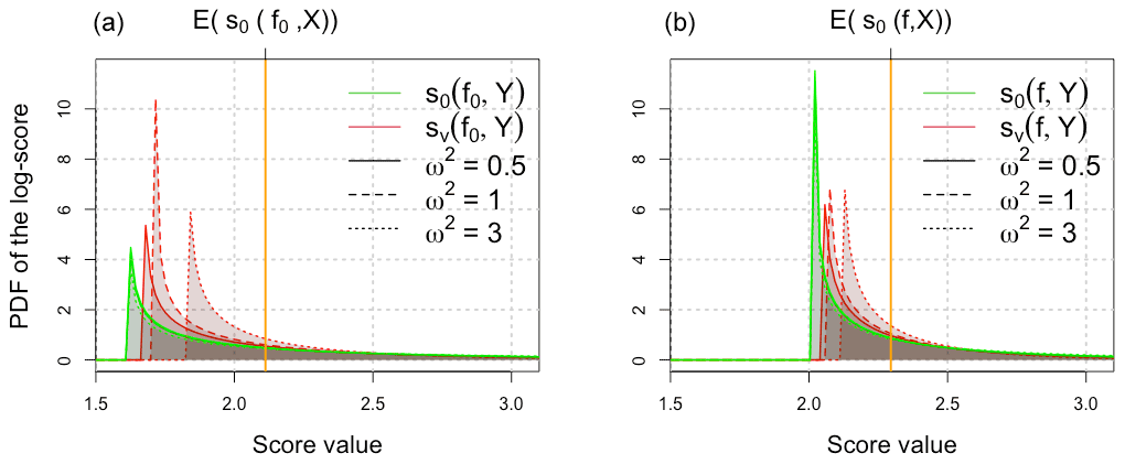
Figure 3 Probability distribution functions (pdfs) from Eq. (9) of the log score used in practice $s_{\mathrm{0}}(.,Y)$ (green) and the proposed score $s_{\vee }(.,Y)$ (red) computed for the perfect forecast f₀ on the left ($\mathit{\mu }={\mathit{\mu }}_{\mathrm{0}}=\mathrm{0}$ and $\mathit{\sigma }={\mathit{\sigma }}_{\mathrm{0}}=\mathrm{2}$) and imperfect forecasts f on the right (μ=1 and σ=3). The mean of the ideal score is depicted with an orange line: (a) 𝔼(s₀(f₀,X)) and (b) 𝔼(s₀(f,X)) on the right. The following distributions are used: $X\sim \mathcal{N}(\mathrm{0},\mathrm{4})$ and $Y\sim \mathcal{N}(\mathrm{0},\mathrm{4}+{\mathit{\omega }}^{\mathrm{2}})$ with several levels of observational noise ω²=0.5, 1, and 3.

Similarly, under the additive Gaussian Model (A), the random variable associated with the proposed CRPS defined by Eq. (8) is written as

$$\begin{array}{}\text{(10)}& \begin{array}{rl}{c}_{\vee }\left(f,Y\right)& =\stackrel{\mathrm{‾}}{Y}+\mathrm{2}{\mathit{\sigma }}_{\mathit{\omega }}\left[\mathit{\varphi }\left({\displaystyle \frac{\stackrel{\mathrm{‾}}{Y}-\mathit{\mu }}{{\mathit{\sigma }}_{\mathit{\omega }}}}\right)-{\displaystyle \frac{\stackrel{\mathrm{‾}}{Y}-\mathit{\mu }}{{\mathit{\sigma }}_{\mathit{\omega }}}}\stackrel{\mathrm{‾}}{\mathrm{\Phi }}\left({\displaystyle \frac{\stackrel{\mathrm{‾}}{Y}-\mathit{\mu }}{{\mathit{\sigma }}_{\mathit{\omega }}}}\right)\right]\\ & -\left[\mathit{\mu }+{\displaystyle \frac{\mathit{\sigma }}{\sqrt{\mathit{\pi }}}}\right],\end{array}\end{array}$$

where ${\mathit{\sigma }}_{\mathit{\omega }}^{\mathrm{2}}={\mathit{\sigma }}^{\mathrm{2}}+\frac{{\mathit{\omega }}^{\mathrm{2}}{\mathit{\sigma }}_{\mathrm{0}}^{\mathrm{2}}}{{\mathit{\sigma }}_{\mathrm{0}}^{\mathrm{2}}+{\mathit{\omega }}^{\mathrm{2}}}$ and the random variable $\stackrel{\mathrm{‾}}{Y}=\frac{{\mathit{\omega }}^{\mathrm{2}}}{{\mathit{\sigma }}_{\mathrm{0}}^{\mathrm{2}}+{\mathit{\omega }}^{\mathrm{2}}}{\mathit{\mu }}_{\mathrm{0}}+\frac{{\mathit{\sigma }}_{\mathrm{0}}^{\mathrm{2}}}{{\mathit{\sigma }}_{\mathrm{0}}^{\mathrm{2}}+{\mathit{\omega }}^{\mathrm{2}}}Y$ follow a Gaussian pdf with mean μ₀ and variance ${\mathit{\sigma }}_{\mathrm{0}}^{\mathrm{2}}\times \frac{{\mathit{\sigma }}_{\mathrm{0}}^{\mathrm{2}}}{{\mathit{\sigma }}_{\mathrm{0}}^{\mathrm{2}}+{\mathit{\omega }}^{\mathrm{2}}}$. The distribution of Eq. (10) does not belong to any known parametric families; however, it is still possible to characterize the score distribution through sampling when the distribution of Y is available. Finally, having access to distributions like Eq. (9) or Eq. (10) gives access to the whole range of uncertainty of the score distributions, helping to derive statistics that are more representative than the mean as pointed out above and to compute confidence intervals without bootstrapping approximations as in Wilks (2010) and Dirkson et al. (2019). Finding adequate representatives of a score distribution that shows reliable discriminative skills is beyond the scope of this work. Nevertheless, in Appendix G we take forward the concept of score distributions and apply it to computing distances between score distributions in order to assess their discriminative skills.

4 Multiplicative Gamma case

The Gaussian assumption is appropriate when dealing with averages, for example, mean temperatures; however, the normal hypothesis cannot be justified for positive and skewed variables such as precipitation intensities. For instance, multiplicative models are often used in hydrology to account for various errors and uncertainty (measurement errors, process uncertainty, and unknown quantities); see Kavetski et al. (2006a, b) and McMillan et al. (2011). An often-used alternative in such cases is to use a Gamma distribution, which works fairly well in practice to represent the bulk of rainfall intensities. Hence, we assume in this section that the true but unobserved X follows a Gamma distribution with parameters α₀ and β₀: $f_X\left(x\right)=\frac{{\mathit{\beta }}_{\mathrm{0}}^{{\mathit{\alpha }}_{\mathrm{0}}}}{\mathrm{\Gamma }\left({\mathit{\alpha }}_{\mathrm{0}}\right)}{x}^{{\mathit{\alpha }}_{\mathrm{0}}-\mathrm{1}}\exp (-{\mathit{\beta }}_{\mathrm{0}}x)$, for x>0. For positive random variables such as precipitation, additive models cannot be used to introduce errors. Instead, we prefer to use a multiplicative model of the type

$$\begin{array}{}\text{(11)}& \text{Model (B)}\left\{\begin{array}{l}X\sim \mathrm{\Gamma }({\mathit{\alpha }}_{\mathrm{0}},{\mathit{\beta }}_{\mathrm{0}}),\\ Y=X\times \mathit{ϵ},\end{array}\right.\end{array}$$

where ϵ is a positive random variable independent of X. To make feasible computations, we model the error ϵ as an inverse Gamma pdf with parameters a and b: $f_{\mathit{ϵ}}\left(u\right)=\frac{b^a}{\mathrm{\Gamma }\left(a\right)}{u}^{-a-\mathrm{1}}\exp \left(-\frac{b}{u}\right),$ for u>0. The basic conjugate prior properties of such Gamma and inverse Gamma distributions allows us to easily derive the pdf $\left[X\right|Y=y]$. Analogously to Sect. 3, we express the log score and CRPS within this multiplicative Gamma model in the following paragraphs.

4.1 Log-score versions

Let us consider a Gamma distribution f with parameters α>0 and β>0 for the prediction. With obvious notations, the log score for this forecast f becomes

$$\begin{array}{}\text{(12)}& s_{\mathrm{0}}(f,x)=(\mathrm{1}-\mathit{\alpha })\log x+\mathit{\beta }x-\mathit{\alpha }\log \mathit{\beta }+\log \mathrm{\Gamma }\left(\mathit{\alpha }\right).\end{array}$$

Under the Gamma multiplicative model (B), the random variable associated with the corrected log scores defined by Eqs. (1) and (12) is expressed as

$$\begin{array}{}\text{(13)}& \begin{array}{rl}{s}_{\vee }(f,Y)& =(\mathrm{1}-\mathit{\alpha })\left(\mathit{\psi }\left({\mathit{\alpha }}_{\mathrm{0}}+a\right)-\log \left({\mathit{\beta }}_{\mathrm{0}}+b/Y\right)\right)\\ & +\mathit{\beta }{\displaystyle \frac{{\mathit{\alpha }}_{\mathrm{0}}+a}{{\mathit{\beta }}_{\mathrm{0}}+b/Y}}-\mathit{\alpha }\log \mathit{\beta }+\log \mathrm{\Gamma }\left(\mathit{\alpha }\right),\end{array}\end{array}$$

where ψ(x) represents the digamma function defined as the logarithmic derivative of the Gamma function, namely, $\mathit{\psi }\left(x\right)=\mathrm{d}\log \mathrm{\Gamma }\left(x\right)/\mathrm{d}x$. Details of the computations are found in Appendix E.

4.2 CRPS versions

For a Gamma forecast with parameters α and β, the corresponding CRPS (see, e.g., Taillardat et al., 2016; Scheuerer and Möller, 2015) is equal to

$$\begin{array}{}\text{(14)}& \begin{array}{rl}{c}_{\mathrm{0}}(f,x)& =\left[{\displaystyle \frac{\mathit{\alpha }}{\mathit{\beta }}}-{\displaystyle \frac{\mathrm{1}}{\mathit{\beta }B(.5,\mathit{\alpha })}}\right]-x\\ & +\mathrm{2}\left[{\displaystyle \frac{x}{\mathit{\beta }}}f\left(x\right)+\left({\displaystyle \frac{\mathit{\alpha }}{\mathit{\beta }}}-x\right)\stackrel{\mathrm{‾}}{F}\left(x\right)\right].\end{array}\end{array}$$

Under the multiplicative Gamma model (B), the random variable associated with the CRPS Eq. (14) corrected by Eq. (1) is expressed as

$$\begin{array}{}\text{(15)}& \begin{array}{rl}{c}_{\vee }(f,Y)& =\left[{\displaystyle \frac{\mathit{\alpha }}{\mathit{\beta }}}-{\displaystyle \frac{\mathrm{1}}{\mathit{\beta }B(\mathrm{5},\mathit{\alpha })}}\right]-{\displaystyle \frac{{\mathit{\alpha }}_{\mathrm{0}}+a}{{\mathit{\beta }}_{\mathrm{0}}+\frac{b}{Y}}}\\ & +\mathrm{2}{\displaystyle \frac{{\mathit{\beta }}^{\mathit{\alpha }-\mathrm{1}}{\left({\mathit{\beta }}_{\mathrm{0}}+b/Y\right)}^{{\mathit{\alpha }}_{\mathrm{0}}+a}}{B\left(\mathit{\alpha },{\mathit{\alpha }}_{\mathrm{0}}+a\right){\left(\mathit{\beta }+{\mathit{\beta }}_{\mathrm{0}}+b/Y\right)}^{\mathit{\alpha }+{\mathit{\alpha }}_{\mathrm{0}}+a}}}\\ & +{\displaystyle \frac{\mathrm{2}{\left({\mathit{\beta }}_{\mathrm{0}}+b/Y\right)}^{{\mathit{\alpha }}_{\mathrm{0}}+a}}{\mathrm{\Gamma }\left(\mathit{\alpha }\right)\mathrm{\Gamma }\left({\mathit{\alpha }}_{\mathrm{0}}+a\right)}}\underset{\mathrm{0}}{\overset{+\mathrm{\infty }}{\int }}\left({\displaystyle \frac{\mathit{\alpha }}{\mathit{\beta }}}-x\right)\\ & \mathrm{\Gamma }(\mathit{\alpha },\mathit{\beta }x)x^{{\mathit{\alpha }}_{\mathrm{0}}+a-\mathrm{1}}\exp \left(-\left({\mathit{\beta }}_{\mathrm{0}}+b/Y\right)x\right)\mathrm{d}x.\end{array}\end{array}$$

Details of the computations are found in Appendix F. Similarly to Sect. 3.3, one can access the range of uncertainty of the proposed scores, Eqs. (13) and (15), when sampling from the distribution of Y is available. As an illustration, Fig. 4 shows the distributions of the three CRPSs presented in this section. Similarly to the previous section, one can see that the benefits of embedding the uncertainty of the verification data are noticeable in the variance reduction of distributions shaded in red and the smaller distance between the bulk of distributions in red and the mean value of the ideal score.

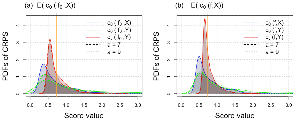
Figure 4 Estimated probability distribution of the CRPS under the multiplicative Gamma model; shown in blue is the distribution of $c_{\mathrm{0}}(.,X)$, shown in green is the distribution of $s_{\mathrm{0}}(.,Y)$, and shown in red is the distribution of $c_{\vee }(.,Y)$, respectively, from Eqs. (14) and (15). The mean of the ideal score $\mathbb{E}\left(c_{\mathrm{0}}\right(.,X\left)\right)$ is depicted with an orange line. (a) Score distributions for the perfect forecast f₀ with the same distribution as X ($\mathit{\alpha }={\mathit{\alpha }}_{\mathrm{0}}=\mathrm{7}$ and $\mathit{\beta }={\mathit{\beta }}_{\mathrm{0}}=\mathrm{2}$) validated against X and corrupted verification data Y with different levels of error: a=7 and 9 and b=8. (b) Score distributions for the imperfect forecast f with distribution parameters α=4 and β=1 validated against X and corrupted verification data Y. The following parameters α₀=7 and β₀=2 are used for the hidden state X.

5 Applications and illustrations

The following section applies and illustrates through simulation studies the benefit of accounting for uncertainty in scores as presented in Sect. 2 through the power analysis of a hypothesis test and the numerical illustration of the motivating example with wind data from Sect. 1. In Appendix G, we illustrate further the consideration of score distributions via the Wasserstein distance.

5.1 Power analysis of hypothesis testing

In this section, a power analysis of the following hypothesis test is performed on simulated data following Diebold and Mariano (2002) in order to investigate the discriminative skills of the proposed score from Eq. (1). In Diebold and Mariano (2002), hypothesis tests focused on discriminating forecasts from the climatology; in the current study, we test the ability of the proposed score to discriminate any forecast f from the perfect forecast f₀ (forecast having the “true” hidden state X distribution). We consider the reference score value of the perfect forecast f₀ to be the mean score evaluated against the true process 𝔼(s₀(f₀,X)). Hypothesis tests are tuned to primarily minimize the error of type I (wrongly rejecting the null hypothesis); consequently, it is common practice to assess the power of a test. The power p is the probability of rejecting a false null hypothesis; the power is expressed as 1−β, where β is the error of type II (failing to reject a false null hypothesis) and is expressed as $p=P\left(\text{Rejecting }{\mathrm{H}}_{\mathrm{0}}\right|{\mathrm{H}}_{\mathrm{1}}\text{ true})$. The closer to 1 the power is, the better the test is at detecting a false null hypothesis. For a given forecast f, the considered hypothesis is expressed as

$$\begin{array}{}\text{(16)}& \left\{\begin{array}{l}{\mathrm{H}}_{\mathrm{0}}:\text{forecast}f\text{is perfect}(f=f_{\mathrm{0}})\\ \text{through the score}s,\\ \text{ leading to }\mathbb{E}\left(s\right(f,.\left)\right)\text{ close to }\mathbb{E}\left(s_{\mathrm{0}}\right(f_{\mathrm{0}},X\left)\right),\\ {\mathrm{H}}_{\mathrm{1}}:\text{forecast}f\text{is imperfect,}\text{leading to}\mathbb{E}\left(s\right(f,.\left)\right)\\ \text{ far from }\mathbb{E}\left(s_{\mathrm{0}}\right(f_{\mathrm{0}},X\left)\right),\end{array}\right.\end{array}$$

where f₀ and f are, respectively, the perfect forecast and an imperfect forecast to be compared with the perfect forecast f₀. In the following, the score $s(f,.)$ will represent, respectively, s₀(f,X), s₀(f,Y), and $s_{\vee }(f,Y)$ in order to compare the ability of the ideal score, the score used in practice, and the proposed score. The parameters associated with the hypothesis are the parameters, μ and σ in the following additive Gaussian model, of the imperfect forecast f, and they are varied to compute the different powers. The statistical test corresponding to Eq. (16) is expressed as

$$\begin{array}{}\text{(17)}& \left\{\begin{array}{l}{\mathrm{H}}_{\mathrm{0}}\text{ is accepted if }t\le c,\\ {\mathrm{H}}_{\mathrm{0}}\text{ is rejected if }t>c,\end{array}\right.\end{array}$$

where $t=\left|\mathbb{E}\right(s(f,.))-\mathbb{E}(s_{\mathrm{0}}(f_{\mathrm{0}},X)\left)\right|$ is the test statistics and c is defined via the error of type I $P(t>c|H_{\mathrm{0}}\text{ is true})=\mathit{\alpha }$ with the level α=0.05 in the present study.

To illustrate this test with numerical simulations, the additive Gaussian Model (A) is considered for the log score, where the forecast, X, and Y are assumed to be normally distributed with an additive error. The expectation in Eq. (17) is approximated and computed over N=1000 verification data points, the true state being X and the corrupted data Y. The approximated test statistic is denoted with $\widehat{t}$. The power p is expressed as $P(\widehat{t}>c|f\text{ is imperfect})$ and is computed over 10 000 samples of length N when parameters μ and σ of the forecast f are varied.

In Fig. 5, the above power p is shown for varying mean μ and standard deviation σ of the forecast f in order to demonstrate the ability of the proposed score $s_{\vee }(.,Y)$ to better discriminate between forecasts than the commonly used score $s_{\mathrm{0}}(.,Y)$. One expects the power to be low around, respectively, μ₀ and σ₀, and as high as possible outside these values. We note that the ideal score s₀ and the proposed score s_∨ have similar power for the test Eq. (17), suggesting similar discriminating skills for both scores. However, the $s_{\mathrm{0}}(.,Y)$ score commonly used in practice results in an ill-behaved power as the observational noise increases (from left to right), indicating the necessity to account for the uncertainty associated with the verification data. The ill-behaved power illustrates the propensity of the test based on $s_{\mathrm{0}}(.,Y)$ to reject H₀ too often and in particular wrongfully when the forecast f is perfect and equals f₀. In addition, the power associated with the score $s_{\mathrm{0}}(.,Y)$ fails to reach the nominal test level α due to the difference in means between $s_{\mathrm{0}}(.,X)$ and $s_{\mathrm{0}}(.,Y)$ ($\mathbb{E}\left(s_{\mathrm{0}}\right(f,X\left)\right)\ne \mathbb{E}\left(s_{\mathrm{0}}\right(f,Y\left)\right)$ for any forecast f) caused by the errors in the verification data Y. This highlights the unreliability of scores evaluated against corrupted verification data. Both varying mean and standard deviation reveal similar conclusions regarding the ability of the proposed score to improve its discriminative skills over a score evaluated on corrupted evaluation data.

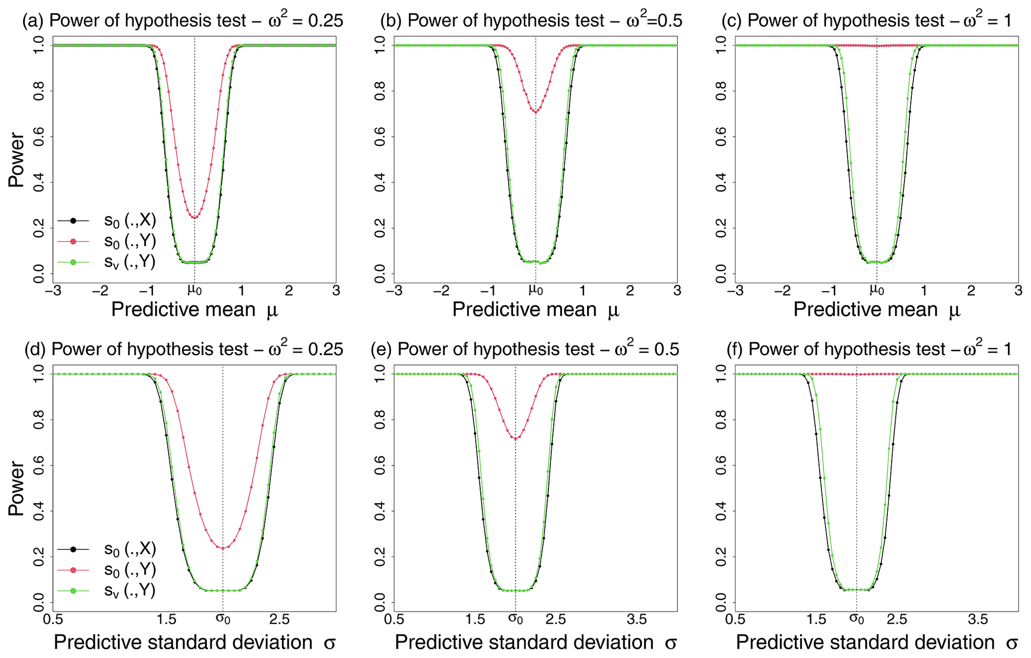
Figure 5 Power of the test Eq. (17) against varying predictive mean μ (a, b, c) and against varying predictive standard deviation σ (d, e, f) of the forecast f for different observational noise levels ω²=0.25 (a, d), ω²=0.5 (b, e), and ω²=1 (c, f). In the simulations, the true state X is distributed as $\mathcal{N}({\mathit{\mu }}_{\mathrm{0}}=\mathrm{0},{\mathit{\sigma }}_{\mathrm{0}}^{\mathrm{2}}=\mathrm{4})$, and Y is distributed as $\mathcal{N}(\mathrm{0},{\mathit{\sigma }}_{\mathrm{0}}^{\mathrm{2}}+{\mathit{\omega }}^{\mathrm{2}})$. The power is expected to be low around μ₀ (or σ₀) and as large as possible elsewhere.

5.2 Application to wind speed prediction

As discussed in the motivating example of Sect. 1, we consider surface wind speed data from the previous work (Bessac et al., 2018) and associated probabilistic distributions. In Bessac et al. (2018), a joint distribution for observations, denoted here as X_ref, and NWP model outputs is proposed and based on Gaussian distributions in a space–time fashion. This joint model aimed at predicting surface wind speed based on the conditional distribution of X_ref given NWP model outputs. The data are Box–Cox-transformed in this study to approximate normal distributions. The model was fitted by maximum likelihood for an area covering parts of Wisconsin, Illinois, Indiana, and Michigan in the United States. In this study, we focus on one station in Wisconsin and recover the parameters of its marginal joint distribution of observations X_ref and NWP outputs from the joint spatiotemporal model. In the following, we evaluate with scores the probability distribution of the NWP model outputs depicted in Fig. 2. In Bessac et al. (2018), the target distribution was the fitted distribution of the observations X_ref; however, in the validation step of the predictive probabilistic model, the observations shown in Fig. 2 were used without accounting for their potential uncertainty and error. This leads to a discrepancy between the target variable X_ref and the verification data that we denote as Y_obs. From Pinson and Hagedorn (2012), a reasonable model for unbiased measurement error in wind speed is ${\mathit{ϵ}}_{\mathrm{obs}}\sim \mathcal{N}(\mathrm{0},\mathrm{0.25})$. Subsequently to Sect. 3, we proposed the following additive framework to account for the observational noise in the scoring framework:

$$\left\{\begin{array}{l}{X}_{\mathrm{ref}}\sim \mathcal{N}({\mathit{\mu }}_{\mathrm{0}},{\mathit{\sigma }}_{\mathrm{0}}^{\mathrm{2}}),{\mathit{\mu }}_{\mathrm{0}}\text{and}{\mathit{\sigma }}_{\mathrm{0}}\text{ retrieved from the joint model},\\ Y_{\mathrm{obs}}=X_{\mathrm{ref}}+{\mathit{ϵ}}_{\mathrm{obs}},\text{ with }{\mathit{ϵ}}_{\mathrm{obs}}\sim \mathcal{N}(\mathrm{0},\mathrm{0.25}),\end{array}\right.$$

where μ₀=2.55 and σ₀=1.23 from the fitted distribution in Bessac et al. (2018). In Table 1, log scores and CRPS are computed as averages over the studied time series in the additive Gaussian case with a previously given formula in Sect. 3. The variance associated with each average score is provided in parentheses. Table 1 shows a significant decrease in the variance when the proposed score is used compared to the score commonly used in practice that does not account for measurement error. One can notice that the variance of the scores used in practice are considerably high, limiting the reliability of these computed scores for decision-making purposes. Additionally, the new mean scores are closer to the ideal mean log score and CRPS, showing the benefit of accounting for observational errors in the scoring framework.

Table 1 Average scores (log score and CRPS) computed for the predictive distribution of the NWP model; the associated standard deviation is given in parentheses. The statistics are computed over the entire studied time series. The mean ideal score 𝔼(s₀(f,X)), the averaged score computed in practice against the measurements 𝔼(s₀(f,Y)), and the proposed score $\mathbb{E}\left(s_{\vee }\right(f,X\left)\right)$ embedding the error in the verification data are computed.

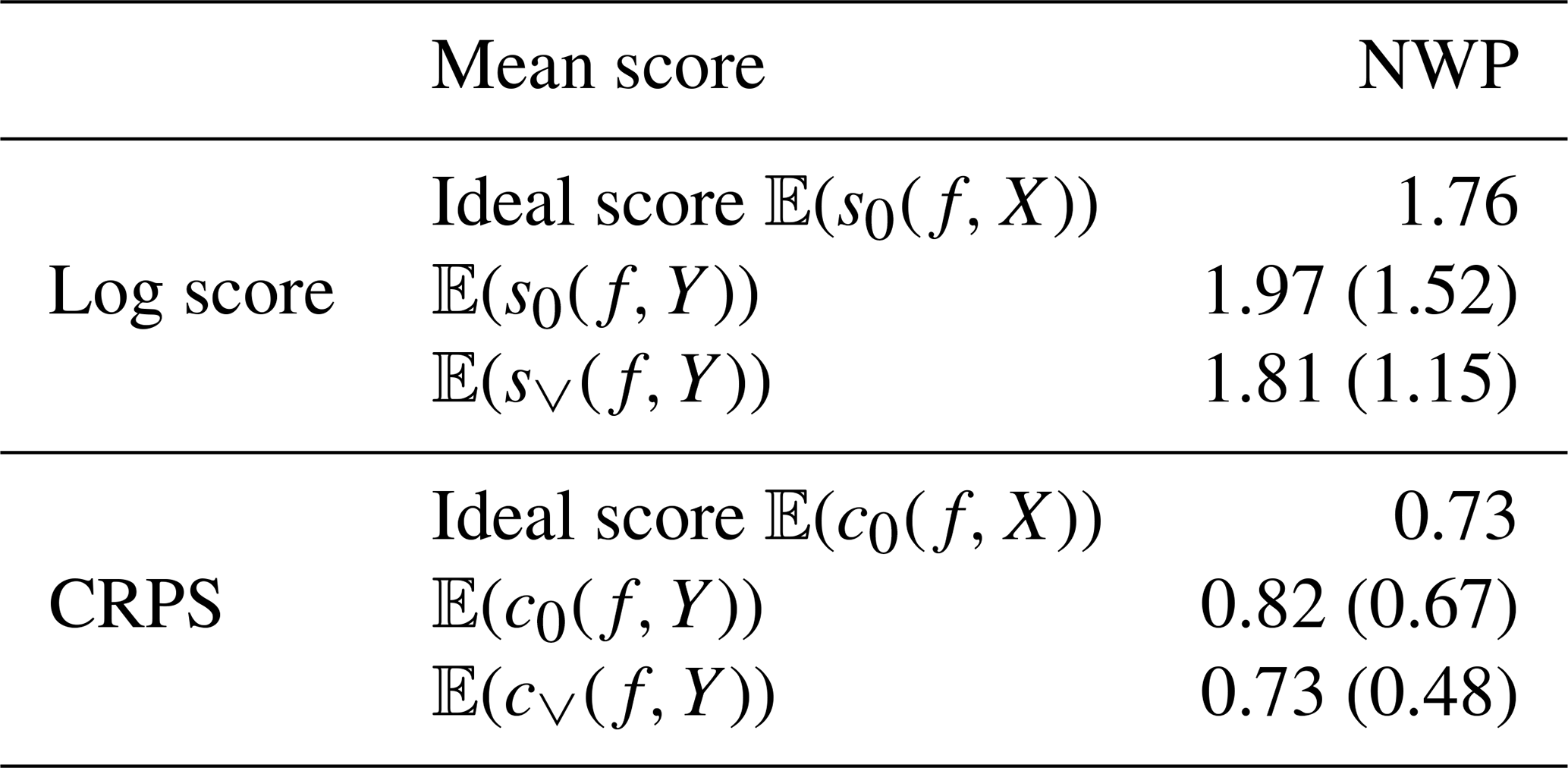
Figure 6 shows the pdf of the scores considered in Table 1; the skewness and the large dispersion in the upper tail illustrate with wind speed data cases where the mean is potentially not an informative summary statistic of the whole distribution. The non-corrected version of the score has a large variance, raising the concern of reliability on scores when computed on error-prone data.

Figure 6 Empirical distribution of uncorrected (green) and corrected scores (red) for the log score (a) and CRPS (b) for the probabilistic distribution NWP model 1 evaluated against observations tainted with uncertainty. The ideal mean score value is illustrated by the orange vertical line.

6 Conclusions

We have quantified, in terms of variance and even distribution, the need to account for the error associated with the verification data when evaluating probabilistic forecasts with scores. An additive framework and a multiplicative framework have been studied in detail to account for the error associated with verification data. Both setups involve a probabilistic model for the accounted errors and a probabilistic description of the underlying non-observed physical process. Although we look only at idealized cases where the involved distributions and their parameters are known, this approach enables us to understand the importance of accounting for the error associated with the verification data.

6.1 Scores with hidden states

The proposed scoring framework was applied to standard additive and multiplicative models for which, via Bayesian conjugacy, the expression of the new scores could be made explicit. However, if the prior on X is not conjugate to the distribution of Y, one can derive approximately the conditional distribution $\left[X\right|Y=y]$ through sampling algorithms such as Markov chain Monte Carlo methods. Additionally, one can relax the assumption of known parameters for the distributions of [X] and [Y|X] by considering priors on the parameters (e.g., priors on μ₀ and σ₀). In practice, we rely on the idea that the climatology and/or information on measurement errors can help express the distribution of X or its priors.

In the current literature on scoring with uncertain verification data, most proposed works rely on additive errors as in Ciach and Krajewski (1999), Saetra et al. (2004), and Mittermaier and Stephenson (2015). Multiplicative error models for various error representations have been proposed in modeling studies, such as for precipitation (McMillan et al., 2011), but have not been considered in scoring correction frameworks. Furthermore, additive and multiplicative state-space models can be generalized to nonlinear and non-Gaussian state-space model specifications; see chap. 7 of Cressie and Wikle (2015) for a discussion and examples. More generally, one could consider the following state-space model specification:

$$\left\{\begin{array}{l}X=f\left(\mathit{\eta }\right),\\ Y=g(X,\mathit{ϵ}),\end{array}\right.$$

where f and g are nonlinear functions describing the hidden state and the state-observation mapping, and η and ϵ are stochastic terms representing, respectively, the stochasticity of the hidden state and the observational error. This generalized specification of the state-observation model could be integrated in future work in the proposed scoring framework via Bayesian specifications of the new score in order to account for prior information on the verification data Y and its uncertainty and priors on the true state X.

6.2 Scores as random variables

Finally, the study raises the important point of investigating the distribution of scores when the verification data are considered to be a random variable. Indeed, investigating the means of scores may not provide sufficient information to compare between score discriminative capabilities. This has been pointed and investigated in Taillardat et al. (2019) in the context of evaluating extremes. This topic has also been extensively discussed by Bolin and Wallin (2019) in the context of varying predictability that generates non-homogeneity in the score values that is poorly represented by an average. One could choose to take into account the uncertainty associated with the inference of distribution parameters and compute different statistics of the distribution rather than the mean. In this case, a Bayesian setup similar to the current work could elegantly integrate the different hierarchies of knowledge, uncertainties, and a priori information to generalize the notion of scores.

Appendix A: Proof of Eq. (2)

For any random variable, say U, its mean can be written conditionally to the random variable y in the following way:

$$\mathbb{E}\left[U\right]=\mathbb{E}\left[\mathbb{E}\left[U|Y=y\right]\right].$$

In our case, the variables $U=s_o(f,X)$ and $s_{\vee }(f,y)=\mathbb{E}\left[U|Y=y\right]$. This gives $\mathbb{E}\left[s_{\vee }(f,Y)\right]=\mathbb{E}\left[s_o(f,X)\right]$. To show the inequality Eq. (2), we use the classical variance decomposition

$$\mathbb{V}\left[U\right]=\mathbb{V}\left[\mathbb{E}\left[U|Y=y\right]\right]+\mathbb{E}\left[\mathbb{V}\left[U|Y=y\right]\right].$$

With our notations, we have

$$\begin{array}{rl}\mathbb{V}\left[s_o(f,X)\right]& =\mathbb{V}\left[\mathbb{E}\left[s_o(f,X)|Y=y\right]\right]\\ & +\mathbb{E}\left[\mathbb{V}\left[s_o(f,X)|Y=y\right]\right]\\ & =\mathbb{V}\left[s_{\vee }(f,Y)\right]+\text{ a non-negative term}.\end{array}$$

This leads to

$$\mathbb{V}\left[s_o(f,X)\right]\ge \mathbb{V}\left[s_{\vee }(f,Y)\right].$$

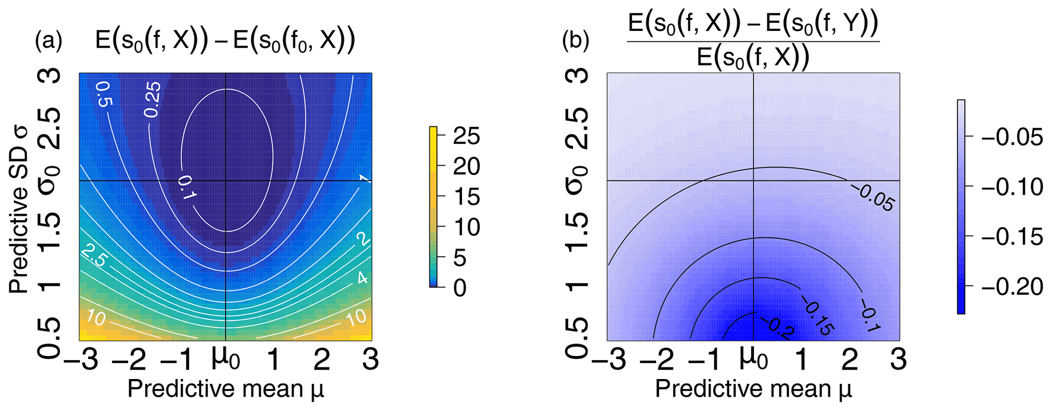
Figure A1 (a) Mean log score for an imperfect forecast f minus the mean log score of the perfect forecast f₀ when evaluated against perfect data X; the imperfect forecast $f\sim \mathcal{N}(\mathit{\mu },\mathit{\sigma })$ has a varying mean μ (x axis) and varying standard deviation σ (y axis). (b) Relative difference between 𝔼(s₀(f,X)) and 𝔼(s₀(f,Y)).

Appendix B: Proof of Eq. (5)

To express the score proposed in Eq. (1), one needs to derive the conditional distribution $\left[X\right|Y=y]$ from Model (A). More precisely, the Gaussian conditional distribution of X given Y=y is equal to

$$\left[X\right|Y=y]\sim \mathcal{N}\left(\stackrel{\mathrm{‾}}{y},{\displaystyle \frac{{\mathit{\omega }}^{\mathrm{2}}{\mathit{\sigma }}_{\mathrm{0}}^{\mathrm{2}}}{{\mathit{\sigma }}_{\mathrm{0}}^{\mathrm{2}}+{\mathit{\omega }}^{\mathrm{2}}}}\right),$$

where $\stackrel{\mathrm{‾}}{y}$ is a weighted sum that updates the prior information about $X\sim \mathcal{N}({\mathit{\mu }}_{\mathrm{0}},{\mathit{\sigma }}_{\mathrm{0}}^{\mathrm{2}})$ with the observation $Y\sim \mathcal{N}({\mathit{\mu }}_{\mathrm{0}},{\mathit{\sigma }}_{\mathrm{0}}^{\mathrm{2}}+{\mathit{\omega }}^{\mathrm{2}})$:

$$\stackrel{\mathrm{‾}}{Y}={\displaystyle \frac{{\mathit{\omega }}^{\mathrm{2}}}{{\mathit{\sigma }}_{\mathrm{0}}^{\mathrm{2}}+{\mathit{\omega }}^{\mathrm{2}}}}{\mathit{\mu }}_{\mathrm{0}}+{\displaystyle \frac{{\mathit{\sigma }}_{\mathrm{0}}^{\mathrm{2}}}{{\mathit{\sigma }}_{\mathrm{0}}^{\mathrm{2}}+{\mathit{\omega }}^{\mathrm{2}}}}Y\sim \mathcal{N}\left({\mathit{\mu }}_{\mathrm{0}},{\mathit{\sigma }}_{\mathrm{0}}^{\mathrm{2}}\times {\displaystyle \frac{{\mathit{\sigma }}_{\mathrm{0}}^{\mathrm{2}}}{{\mathit{\sigma }}_{\mathrm{0}}^{\mathrm{2}}+{\mathit{\omega }}^{\mathrm{2}}}}\right).$$

Combining this information with Eqs. (1) and (3) leads to

$$\begin{array}{rl}{s}_{\vee }(f,y)& =\log \mathit{\sigma }+{\displaystyle \frac{\mathrm{1}}{\mathrm{2}{\mathit{\sigma }}^{\mathrm{2}}}}\left\{\mathbb{E}\left[(X-\mathit{\mu }{)}^{\mathrm{2}}|Y=y\right]\right\}+{\displaystyle \frac{\mathrm{1}}{\mathrm{2}}}\log \mathrm{2}\mathit{\pi }\\ & =\log \mathit{\sigma }+{\displaystyle \frac{\mathrm{1}}{\mathrm{2}{\mathit{\sigma }}^{\mathrm{2}}}}\left\{\mathbb{V}\left[X\right|Y=y]+{\left(\mathbb{E}\left[X\right|Y=y]-\mathit{\mu }\right)}^{\mathrm{2}}\right\}\\ & +{\displaystyle \frac{\mathrm{1}}{\mathrm{2}}}\log \mathrm{2}\mathit{\pi }\\ & =\log \mathit{\sigma }+{\displaystyle \frac{\mathrm{1}}{\mathrm{2}{\mathit{\sigma }}^{\mathrm{2}}}}\mathit{\{}{\displaystyle \frac{{\mathit{\omega }}^{\mathrm{2}}{\mathit{\sigma }}_{\mathrm{0}}^{\mathrm{2}}}{{\mathit{\sigma }}_{\mathrm{0}}^{\mathrm{2}}+{\mathit{\omega }}^{\mathrm{2}}}}\\ & +{\left({\displaystyle \frac{{\mathit{\omega }}^{\mathrm{2}}}{{\mathit{\sigma }}_{\mathrm{0}}^{\mathrm{2}}+{\mathit{\omega }}^{\mathrm{2}}}}{\mathit{\mu }}_{\mathrm{0}}+{\displaystyle \frac{{\mathit{\sigma }}_{\mathrm{0}}^{\mathrm{2}}}{{\mathit{\sigma }}_{\mathrm{0}}^{\mathrm{2}}+{\mathit{\omega }}^{\mathrm{2}}}}y-\mathit{\mu }\right)}^{\mathrm{2}}\mathit{\}}+{\displaystyle \frac{\mathrm{1}}{\mathrm{2}}}\log \mathrm{2}\mathit{\pi }.\end{array}$$

By construction, we have

$${\mathbb{E}}_Y\left(s_{\vee }(f,Y)\right)={\mathbb{E}}_{\stackrel{\mathrm{‾}}{Y}}\left(s_{\vee }(f,\stackrel{\mathrm{‾}}{Y})\right)={\mathbb{E}}_X\left(s_{\mathrm{0}}(f,X)\right).$$

This means that, to obtain the right score value, we can first compute $\stackrel{\mathrm{‾}}{Y}$ as the best estimator of the unobserved X and then use it in the corrected score $s_{\vee }(f,\stackrel{\mathrm{‾}}{Y})$.

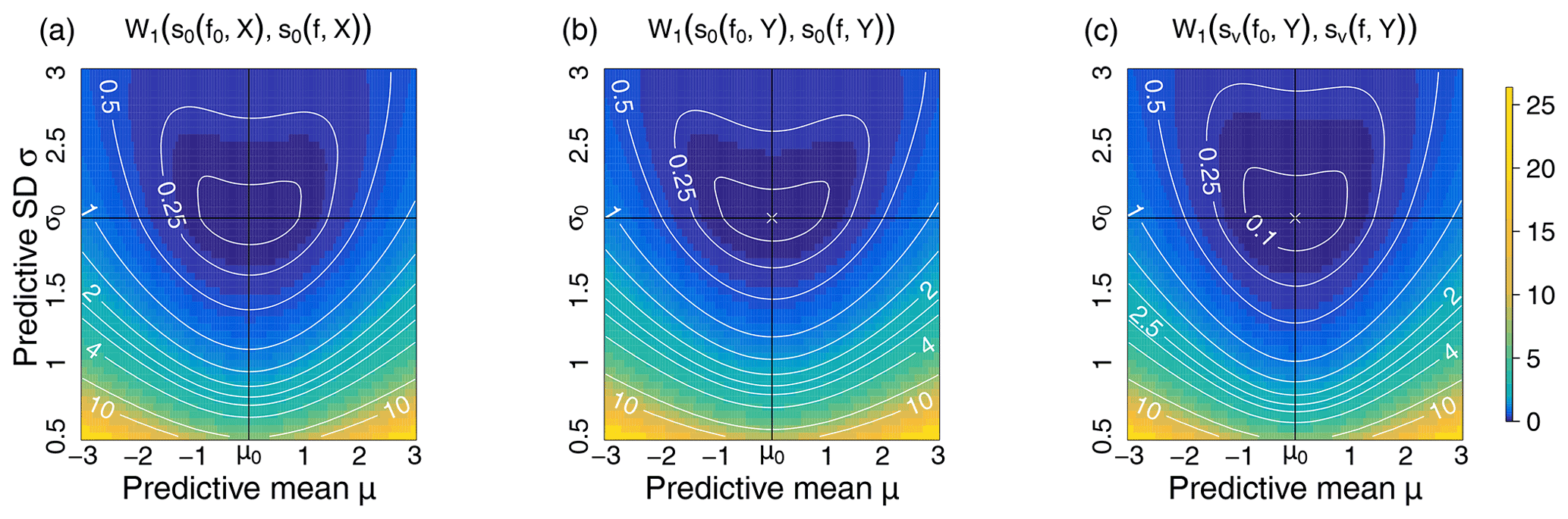
Figure B1 Bottom row: Wasserstein distance $W_{\mathrm{1}}\left(s_{\mathrm{0}}\right(f_{\mathrm{0}},.),s_{\mathrm{0}}(f,.\left)\right)$ between log-score s₀ distributions evaluated at the perfect forecast f₀ and the imperfect forecast f with varying predictive mean μ (x axis) and varying predictive standard deviation σ (y axis). From (a) to (c): log scores are evaluated against the hidden true state X via s₀(f,X), against Y tainted by observational noise of level ω²=1 via s₀(f,Y) and through the corrected log-score version $s_{\vee }(f,Y)$. The verification data X and perfect forecast f₀ are distributed according to $f_{\mathrm{0}}\sim \mathcal{N}(\mathrm{0},\mathrm{4})$. On the central and right surfaces, the white cross “X” indicates the numerical minimum of each surface.

Appendix C: Proof of Eq. (8)

To compute the corrected CRPS, one needs to calculate the conditional expectation of c₀(f,X) under the distribution of $\left[X\right|Y=y]$. We first compute the expectation E(c₀(f,X)) and then substitute X by $\stackrel{\mathrm{‾}}{Y}$ and its distribution with mean $a=\stackrel{\mathrm{‾}}{y}$ and standard deviation $b=\sqrt{\frac{{\mathit{\omega }}^{\mathrm{2}}{\mathit{\sigma }}_{\mathrm{0}}^{\mathrm{2}}}{{\mathit{\sigma }}_{\mathrm{0}}^{\mathrm{2}}+{\mathit{\omega }}^{\mathrm{2}}}}$. From Eq. (7) we obtain

$$\begin{array}{rl}\mathbb{E}\left(c_{\mathrm{0}}\right(f,X\left)\right)& =\mathbb{E}\left(X\right)+\mathrm{2}\mathit{\sigma }[\mathbb{E}\left(\mathit{\varphi }\left({\displaystyle \frac{X-\mathit{\mu }}{\mathit{\sigma }}}\right)\right)\\ & -\mathbb{E}\left({\displaystyle \frac{X-\mathit{\mu }}{\mathit{\sigma }}}\stackrel{\mathrm{‾}}{{\mathrm{\Phi }}_{\mathrm{0}}}\left({\displaystyle \frac{X-\mathit{\mu }}{\mathit{\sigma }}}\right)\right)]-\left[\mathit{\mu }+{\displaystyle \frac{\mathit{\sigma }}{\sqrt{\mathit{\pi }}}}\right].\end{array}$$

If X follows a normal distribution with mean a and variance b², that is, $X=a+bZ$ with Z a standard random variable, then we can define the continuous function $h\left(z\right)=\stackrel{\mathrm{‾}}{\mathrm{\Phi }}\left(\frac{a+bz-\mathit{\mu }}{\mathit{\sigma }}\right),$ with $h^{\prime }\left(z\right)=-\frac{b}{\mathit{\sigma }}\mathit{\varphi }\left(\frac{a+bz-\mathit{\mu }}{\mathit{\sigma }}\right).$ Then, we apply Stein's lemma (Stein, 1981), which states that $\mathbb{E}\left[h^{\prime }\left(Z\right)\right]=\mathbb{E}\left[Zh\left(Z\right)\right]$, because Z is a standard random variable. It follows with the notations $t=\frac{b^{\mathrm{2}}}{\mathrm{2}{\mathit{\sigma }}^{\mathrm{2}}}$ and $\mathit{\lambda }=\frac{a-\mathit{\mu }}{\mathit{\sigma }}$ that

$$\begin{array}{rl}\mathbb{E}\left[{\displaystyle \frac{X-\mathit{\mu }}{\mathit{\sigma }}}\stackrel{\mathrm{‾}}{\mathrm{\Phi }}\left({\displaystyle \frac{X-\mathit{\mu }}{\mathit{\sigma }}}\right)\right]& =\mathit{\lambda }\mathbb{E}\left[\stackrel{\mathrm{‾}}{\mathrm{\Phi }}\left(\mathit{\lambda }+{\displaystyle \frac{b}{\mathit{\sigma }}}Z\right)\right]\\ & +{\displaystyle \frac{b}{\mathit{\sigma }}}\mathbb{E}\left[Zh\left(Z\right)\right],\\ & =\mathit{\lambda }\mathbb{E}\left(\mathbb{P}\left[Z^{\prime }>\left(\mathit{\lambda }+{\displaystyle \frac{b}{\mathit{\sigma }}}Z\right)\right]\right)\\ & +{\displaystyle \frac{b}{\mathit{\sigma }}}\mathbb{E}\left[h^{\prime }\left(Z\right)\right],\end{array}$$

where Z^′ has a standard normal distribution

$$=\mathit{\lambda }\mathbb{E}\left(\mathbb{P}\left[Z^{\prime }-{\displaystyle \frac{b}{\mathit{\sigma }}}Z>\mathit{\lambda }\right]\right)-{\displaystyle \frac{b^{\mathrm{2}}}{{\mathit{\sigma }}^{\mathrm{2}}}}\mathbb{E}\left[\mathit{\varphi }\left({\displaystyle \frac{a+bZ-\mathit{\mu }}{\mathit{\sigma }}}\right)\right],$$

with

$$\begin{array}{rl}\mathit{\lambda }\mathbb{P}\left[Z^{\prime }-{\displaystyle \frac{b}{\mathit{\sigma }}}Z>\mathit{\lambda }\right]& =\mathit{\lambda }\stackrel{\mathrm{‾}}{\mathrm{\Phi }}\left[{\displaystyle \frac{\mathit{\lambda }}{\sqrt{\mathrm{1}+b^{\mathrm{2}}/{\mathit{\sigma }}^{\mathrm{2}}}}}\right]\\ & =\mathit{\lambda }\stackrel{\mathrm{‾}}{\mathrm{\Phi }}\left[{\displaystyle \frac{a-\mathit{\mu }}{\sqrt{{\mathit{\sigma }}^{\mathrm{2}}+b^{\mathrm{2}}}}}\right]\\ & ={\displaystyle \frac{a-\mathit{\mu }}{\mathit{\sigma }}}\stackrel{\mathrm{‾}}{\mathrm{\Phi }}\left[{\displaystyle \frac{a-\mathit{\mu }}{\sqrt{{\mathit{\sigma }}^{\mathrm{2}}+b^{\mathrm{2}}}}}\right].\end{array}$$

Then

$$\begin{array}{rl}\mathbb{E}\left[{\displaystyle \frac{X-\mathit{\mu }}{\mathit{\sigma }}}\stackrel{\mathrm{‾}}{\mathrm{\Phi }}\left({\displaystyle \frac{X-\mathit{\mu }}{\mathit{\sigma }}}\right)\right]& ={\displaystyle \frac{a-\mathit{\mu }}{\mathit{\sigma }}}\stackrel{\mathrm{‾}}{\mathrm{\Phi }}\left[{\displaystyle \frac{a-\mathit{\mu }}{\sqrt{{\mathit{\sigma }}^{\mathrm{2}}+b^{\mathrm{2}}}}}\right]\\ & -{\displaystyle \frac{b^{\mathrm{2}}}{{\mathit{\sigma }}^{\mathrm{2}}}}\mathbb{E}\left[\mathit{\varphi }\left({\displaystyle \frac{a+bZ-\mathit{\mu }}{\mathit{\sigma }}}\right)\right]\end{array}$$

and

$$\begin{array}{rl}\mathbb{E}\left[\mathit{\varphi }\left({\displaystyle \frac{a+bZ-\mathit{\mu }}{\mathit{\sigma }}}\right)\right]& ={\displaystyle \frac{\mathrm{1}}{\sqrt{\mathrm{2}\mathit{\pi }}}}\mathbb{E}\left(\exp \left(-{\displaystyle \frac{\mathrm{1}}{\mathrm{2}}}{\left({\displaystyle \frac{a+bZ-\mathit{\mu }}{\mathit{\sigma }}}\right)}^{\mathrm{2}}\right)\right)\\ & ={\displaystyle \frac{\mathrm{1}}{\sqrt{\mathrm{2}\mathit{\pi }}}}\mathbb{E}\left(\exp \left(-{\displaystyle \frac{b^{\mathrm{2}}}{\mathrm{2}{\mathit{\sigma }}^{\mathrm{2}}}}{\left(Z+{\displaystyle \frac{a-\mathit{\mu }}{b}}\right)}^{\mathrm{2}}\right)\right).\end{array}$$

${\left(Z+\frac{(a-\mathit{\mu })}{b}\right)}^{\mathrm{2}}$ is a non-centered chi-squared distribution with 1 degree of freedom and a non-central parameter $(\frac{a-\mathit{\mu }}{b}{)}^{\mathrm{2}}$ with a known moment-generating function

$$G\left(t;k=\mathrm{1},\mathit{\lambda }={\left({\displaystyle \frac{a-\mathit{\mu }}{b}}\right)}^{\mathrm{2}}\right)={\displaystyle \frac{\exp \left(\frac{\mathit{\lambda }t}{\mathrm{1}-\mathrm{2}t}\right)}{(\mathrm{1}-\mathrm{2}t{)}^{k/\mathrm{2}}}}.$$

It follows that

$$\begin{array}{rl}\mathbb{E}\left[\mathit{\varphi }\left({\displaystyle \frac{a+bZ-\mathit{\mu }}{\mathit{\sigma }}}\right)\right]& ={\displaystyle \frac{\mathrm{1}}{\sqrt{\mathrm{2}\mathit{\pi }}}}\\ & G\left(t={\displaystyle \frac{-b^{\mathrm{2}}}{\mathrm{2}{\mathit{\sigma }}^{\mathrm{2}}}};k=\mathrm{1},\mathit{\lambda }={\left({\displaystyle \frac{a-\mathit{\mu }}{b}}\right)}^{\mathrm{2}}\right)\\ & ={\displaystyle \frac{\mathrm{1}}{\sqrt{\mathrm{2}\mathit{\pi }}}}{\displaystyle \frac{\exp \left(\frac{\frac{-(a-\mathit{\mu }{)}^{\mathrm{2}}}{b^{\mathrm{2}}}\frac{b^{\mathrm{2}}}{\mathrm{2}{\mathit{\sigma }}^{\mathrm{2}}}}{\mathrm{1}+\frac{b^{\mathrm{2}}}{{\mathit{\sigma }}^{\mathrm{2}}}}\right)}{\sqrt{\left(\mathrm{1}+\frac{b^{\mathrm{2}}}{{\mathit{\sigma }}^{\mathrm{2}}}\right)}}}\\ & ={\displaystyle \frac{\mathit{\sigma }}{\sqrt{\mathrm{2}\mathit{\pi }}\sqrt{{\mathit{\sigma }}^{\mathrm{2}}+b^{\mathrm{2}}}}}\\ & \exp \left({\displaystyle \frac{-(a-\mathit{\mu }{)}^{\mathrm{2}}}{\mathrm{2}\left({\mathit{\sigma }}^{\mathrm{2}}+b^{\mathrm{2}}\right)}}\right).\end{array}$$

We obtain

$$\begin{array}{rl}E\left(c_{\mathrm{0}}\right(f,X\left)\right)& =E\left(X\right)+\mathrm{2}\mathit{\sigma }[\left(\mathrm{1}+{\displaystyle \frac{b^{\mathrm{2}}}{{\mathit{\sigma }}^{\mathrm{2}}}}\right)E\left(\mathit{\varphi }\left({\displaystyle \frac{X-\mathit{\mu }}{\mathit{\sigma }}}\right)\right)\\ & -{\displaystyle \frac{a-\mathit{\mu }}{\mathit{\sigma }}}\stackrel{\mathrm{‾}}{\mathrm{\Phi }}\left[{\displaystyle \frac{a-\mathit{\mu }}{\sqrt{{\mathit{\sigma }}^{\mathrm{2}}+b^{\mathrm{2}}}}}\right]]-\left(\mathit{\mu }+{\displaystyle \frac{\mathit{\sigma }}{\sqrt{\mathit{\pi }}}}\right)\\ & =E\left(X\right)+\mathrm{2}\mathit{\sigma }[\left(\mathrm{1}+{\displaystyle \frac{b^{\mathrm{2}}}{{\mathit{\sigma }}^{\mathrm{2}}}}\right){\displaystyle \frac{\mathit{\sigma }}{\sqrt{\mathrm{2}\mathit{\pi }({\mathit{\sigma }}^{\mathrm{2}}+b^{\mathrm{2}})}}}\\ & \exp \left({\displaystyle \frac{-(a-\mathit{\mu }{)}^{\mathrm{2}}}{\mathrm{2}({\mathit{\sigma }}^{\mathrm{2}}+b^{\mathrm{2}})}}\right)-{\displaystyle \frac{a-\mathit{\mu }}{\mathit{\sigma }}}\stackrel{\mathrm{‾}}{\mathrm{\Phi }}\left[{\displaystyle \frac{a-\mathit{\mu }}{\sqrt{{\mathit{\sigma }}^{\mathrm{2}}+b^{\mathrm{2}}}}}\right]]\\ & -\left(\mathit{\mu }+{\displaystyle \frac{\mathit{\sigma }}{\sqrt{\mathit{\pi }}}}\right)\\ & =E\left(X\right)+\mathrm{2}[{\displaystyle \frac{\sqrt{{\mathit{\sigma }}^{\mathrm{2}}+b^{\mathrm{2}}}}{\sqrt{\mathrm{2}\mathit{\pi }}}}\exp \left({\displaystyle \frac{-(a-\mathit{\mu }{)}^{\mathrm{2}}}{\mathrm{2}({\mathit{\sigma }}^{\mathrm{2}}+b^{\mathrm{2}})}}\right)\\ & -(a-\mathit{\mu })\stackrel{\mathrm{‾}}{\mathrm{\Phi }}\left[{\displaystyle \frac{a-\mathit{\mu }}{\sqrt{{\mathit{\sigma }}^{\mathrm{2}}+b^{\mathrm{2}}}}}\right]]\\ & -\left(\mathit{\mu }+{\displaystyle \frac{\mathit{\sigma }}{\sqrt{\mathit{\pi }}}}\right).\end{array}$$

The expression of Eq. (8) is obtained by substituting X with $\stackrel{\mathrm{‾}}{Y}$ and its Gaussian distribution with mean $a=\stackrel{\mathrm{‾}}{y}$ and standard deviation $b=\sqrt{\frac{{\mathit{\omega }}^{\mathrm{2}}{\mathit{\sigma }}_{\mathrm{0}}^{\mathrm{2}}}{{\mathit{\sigma }}_{\mathrm{0}}^{\mathrm{2}}+{\mathit{\omega }}^{\mathrm{2}}}}$ in the expression Eq. (6). This gives

$$\begin{array}{rl}{c}_{\vee }(f,\stackrel{\mathrm{‾}}{y})& =E\left(c_{\mathrm{0}}\right(f,X\left)\right|Y=y)\\ & =\stackrel{\mathrm{‾}}{y}-\left(\mathit{\mu }+{\displaystyle \frac{\mathit{\sigma }}{\sqrt{\mathit{\pi }}}}\right)\\ & +\mathrm{2}\left({\displaystyle \frac{\sqrt{{\mathit{\sigma }}^{\mathrm{2}}+\frac{{\mathit{\sigma }}_{\mathrm{0}}^{\mathrm{2}}{\mathit{\omega }}^{\mathrm{2}}}{{\mathit{\sigma }}_{\mathrm{0}}^{\mathrm{2}}+{\mathit{\omega }}^{\mathrm{2}}}}}{\sqrt{\mathrm{2}\mathit{\pi }}}}\exp \left(-{\displaystyle \frac{(\stackrel{\mathrm{‾}}{y}-\mathit{\mu }{)}^{\mathrm{2}}}{\mathrm{2}({\mathit{\sigma }}^{\mathrm{2}}+\frac{{\mathit{\omega }}^{\mathrm{2}}{\mathit{\sigma }}_{\mathrm{0}}^{\mathrm{2}}}{{\mathit{\sigma }}_{\mathrm{0}}^{\mathrm{2}}+{\mathit{\omega }}^{\mathrm{2}}})}}\right)\right.\\ & \left.-\left(\stackrel{\mathrm{‾}}{y}-\mathit{\mu }\right)\mathrm{\Phi }\left({\displaystyle \frac{\stackrel{\mathrm{‾}}{y}-\mathit{\mu }}{\sqrt{{\mathit{\sigma }}^{\mathrm{2}}+\frac{{\mathit{\omega }}^{\mathrm{2}}{\mathit{\sigma }}_{\mathrm{0}}^{\mathrm{2}}}{{\mathit{\sigma }}_{\mathrm{0}}^{\mathrm{2}}+{\mathit{\omega }}^{\mathrm{2}}}}}}\right)\right).\end{array}$$

Appendix D: Proof of Eq. (9)

For Model (A), both random variables Y and $\stackrel{\mathrm{‾}}{Y}=\frac{{\mathit{\omega }}^{\mathrm{2}}}{{\mathit{\sigma }}_{\mathrm{0}}^{\mathrm{2}}+{\mathit{\omega }}^{\mathrm{2}}}{\mathit{\mu }}_{\mathrm{0}}+\frac{{\mathit{\sigma }}_{\mathrm{0}}^{\mathrm{2}}}{{\mathit{\sigma }}_{\mathrm{0}}^{\mathrm{2}}+{\mathit{\omega }}^{\mathrm{2}}}Y$ are normally distributed with the same mean μ₀ but different variances, ${\mathit{\sigma }}_{\mathrm{0}}^{\mathrm{2}}+{\mathit{\omega }}^{\mathrm{2}}$ and ${\left(\frac{{\mathit{\sigma }}_{\mathrm{0}}^{\mathrm{2}}}{{\mathit{\sigma }}_{\mathrm{0}}^{\mathrm{2}}+{\mathit{\omega }}^{\mathrm{2}}}\right)}^{\mathrm{2}}({\mathit{\sigma }}_{\mathrm{0}}^{\mathrm{2}}+{\mathit{\omega }}^{\mathrm{2}})$, respectively. Since a chi-squared distribution can be defined as the square of a Gaussian random variable, it follows from Eq. (5) that

$$s_{\mathrm{0}}\left(f,Y\right)\stackrel{d}{=}{a}_{\mathrm{0}}+b_{\mathrm{0}}{\mathit{\chi }}_{\mathrm{0}}^{\mathrm{2}}\text{ and }{s}_{\vee }\left(f,Y\right)\stackrel{d}{=}{a}_{\vee }+b_{\vee }{\mathit{\chi }}_{\vee }^{\mathrm{2}},$$

where $\stackrel{d}{=}$ means equality in distribution and

$$\begin{array}{c}{\displaystyle }{a}_{\mathrm{0}}=\log \mathit{\sigma }+{\displaystyle \frac{\mathrm{1}}{\mathrm{2}}}\log \mathrm{2}\mathit{\pi }\text{ and }{b}_{\mathrm{0}}={\displaystyle \frac{{\mathit{\sigma }}_{\mathrm{0}}^{\mathrm{2}}+{\mathit{\omega }}^{\mathrm{2}}}{\mathrm{2}{\mathit{\sigma }}^{\mathrm{2}}}},\\ {\displaystyle }{a}_{\vee }=\log \mathit{\sigma }+{\displaystyle \frac{\mathrm{1}}{\mathrm{2}{\mathit{\sigma }}^{\mathrm{2}}}}{\displaystyle \frac{{\mathit{\omega }}^{\mathrm{2}}{\mathit{\sigma }}_{\mathrm{0}}^{\mathrm{2}}}{{\mathit{\sigma }}_{\mathrm{0}}^{\mathrm{2}}+{\mathit{\omega }}^{\mathrm{2}}}}+{\displaystyle \frac{\mathrm{1}}{\mathrm{2}}}\log \mathrm{2}\mathit{\pi }\text{ and }\\ {\displaystyle }{b}_{\vee }={\displaystyle \frac{{\mathit{\sigma }}_{\mathrm{0}}^{\mathrm{2}}+{\mathit{\omega }}^{\mathrm{2}}}{\mathrm{2}{\mathit{\sigma }}^{\mathrm{2}}}}{\left({\displaystyle \frac{{\mathit{\sigma }}_{\mathrm{0}}^{\mathrm{2}}}{{\mathit{\sigma }}_{\mathrm{0}}^{\mathrm{2}}+{\mathit{\omega }}^{\mathrm{2}}}}\right)}^{\mathrm{2}},\end{array}$$

with ${\mathit{\chi }}_{\mathrm{0}}^{\mathrm{2}}$ and ${\mathit{\chi }}_{\vee }^{\mathrm{2}}$ representing a non-central chi-squared random variable with 1 degree of freedom and a non-centrality parameter:

$${\mathit{\lambda }}_{\mathrm{0}}={\displaystyle \frac{({\mathit{\mu }}_{\mathrm{0}}-\mathit{\mu }{)}^{\mathrm{2}}}{{\mathit{\sigma }}_{\mathrm{0}}^{\mathrm{2}}+{\mathit{\omega }}^{\mathrm{2}}}}\text{ and }{\mathit{\lambda }}_{\vee }={\displaystyle \frac{({\mathit{\mu }}_{\mathrm{0}}-\mathit{\mu }{)}^{\mathrm{2}}}{{\mathit{\sigma }}_{\mathrm{0}}^{\mathrm{2}}+{\mathit{\omega }}^{\mathrm{2}}}}{\left({\displaystyle \frac{{\mathit{\sigma }}_{\mathrm{0}}^{\mathrm{2}}+{\mathit{\omega }}^{\mathrm{2}}}{{\mathit{\sigma }}_{\mathrm{0}}^{\mathrm{2}}}}\right)}^{\mathrm{2}}.$$

Appendix E: Proof of Eq. (13)

In Model (B), the basic conjugate prior properties of such Gamma and inverse Gamma distributions allow us to say that $\left[X\right|Y=y]$ now follows a Gamma distribution with parameters α₀+a and ${\mathit{\beta }}_{\mathrm{0}}+b/y$:

$$\begin{array}{rl}{f}_{X|Y=y}\left(x\right|y)& ={\displaystyle \frac{{\left({\mathit{\beta }}_{\mathrm{0}}+b/y\right)}^{{\mathit{\alpha }}_{\mathrm{0}}+a}}{\mathrm{\Gamma }\left({\mathit{\alpha }}_{\mathrm{0}}+a\right)}}{x}^{{\mathit{\alpha }}_{\mathrm{0}}+a-\mathrm{1}}\\ & \exp \left(-x\left({\mathit{\beta }}_{\mathrm{0}}+b/y\right)\right),\text{for}x>\mathrm{0}.\end{array}$$

It follows that the proposed corrected score is

$$\begin{array}{rl}{s}_{\vee }(f,y)& =\mathbb{E}\left[s_o(f,X)|Y=y\right]\\ & =(\mathrm{1}-\mathit{\alpha })\mathbb{E}\left[\log \left(X\right)|Y=y\right]\\ & +\mathit{\beta }\mathbb{E}\left[X|Y=y\right]-\mathit{\alpha }\log \mathit{\beta }+\log \mathrm{\Gamma }\left(\mathit{\alpha }\right),\\ & =(\mathrm{1}-\mathit{\alpha })\left(\mathit{\psi }({\mathit{\alpha }}_{\mathrm{0}}+a)-\log \left({\mathit{\beta }}_{\mathrm{0}}+{\displaystyle \frac{b}{y}}\right)\right)\\ & +\mathit{\beta }{\displaystyle \frac{{\mathit{\alpha }}_{\mathrm{0}}+a}{{\mathit{\beta }}_{\mathrm{0}}+\frac{b}{y}}}-\mathit{\alpha }\log \mathit{\beta }+\log \mathrm{\Gamma }\left(\mathit{\alpha }\right).\end{array}$$

Indeed, $\mathbb{E}\left[X|Y=y\right]=\frac{{\mathit{\alpha }}_{\mathrm{0}}+a}{{\mathit{\beta }}_{\mathrm{0}}+\frac{b}{y}}$ and $\mathbb{E}\left[\log \left(X\right)|Y=y\right]=\mathit{\psi }({\mathit{\alpha }}_{\mathrm{0}}+a)-\log \left({\mathit{\beta }}_{\mathrm{0}}+\frac{b}{y}\right)$, where ψ(x) represents the digamma function defined as the logarithmic derivative of the Gamma function, namely, $\mathit{\psi }\left(x\right)=\mathrm{d}\log \mathrm{\Gamma }\left(x\right)/\mathrm{d}x$.

Appendix F: Proof of Eq. (15)

From Eq. (14) we obtain

$$\begin{array}{rl}{c}_{\vee }(f,y)& =\mathbb{E}\left[X|Y=y\right]-\left[{\displaystyle \frac{\mathit{\alpha }}{\mathit{\beta }}}+{\displaystyle \frac{\mathrm{1}}{\mathit{\beta }B(.5,\mathit{\alpha })}}\right]\\ & +\mathrm{2}[\mathbb{E}\left[{\displaystyle \frac{X}{\mathit{\beta }}}f\left(X\right)|Y=y\right]\\ & +\mathbb{E}\left[\left({\displaystyle \frac{\mathit{\alpha }}{\mathit{\beta }}}-X\right)\stackrel{\mathrm{‾}}{F}\left(X\right)|Y=y\right]].\end{array}$$

Since the conditional distribution of $\left[X\right|Y=y]$ is known,

$$\begin{array}{rl}\mathbb{E}\left[{\displaystyle \frac{X}{\mathit{\beta }}}f\left(X\right)|Y=y\right]& ={\displaystyle \frac{\mathrm{1}}{\mathit{\beta }}}\underset{\mathrm{0}}{\overset{+\mathrm{\infty }}{\int }}xf\left(x\right){\displaystyle \frac{({\mathit{\beta }}_{\mathrm{0}}+b/y{)}^{{\mathit{\alpha }}_{\mathrm{0}}+a}}{\mathrm{\Gamma }({\mathit{\alpha }}_{\mathrm{0}}+a)}}{x}^{{\mathit{\alpha }}_{\mathrm{0}}+a-\mathrm{1}}\\ & \exp \left(-x({\mathit{\beta }}_{\mathrm{0}}+b/y)\right)\mathrm{d}x\\ & ={\displaystyle \frac{{\mathit{\beta }}^{\mathit{\alpha }-\mathrm{1}}{\left({\mathit{\beta }}_{\mathrm{0}}+b/y\right)}^{{\mathit{\alpha }}_{\mathrm{0}}+a}}{\mathrm{\Gamma }\left(\mathit{\alpha }\right)\mathrm{\Gamma }\left({\mathit{\alpha }}_{\mathrm{0}}+a\right)}}\underset{\mathrm{0}}{\overset{+\mathrm{\infty }}{\int }}{x}^{\mathit{\alpha }+{\mathit{\alpha }}_{\mathrm{0}}+a-\mathrm{1}}\\ & \exp \left(-\left(\mathit{\beta }+{\mathit{\beta }}_{\mathrm{0}}+b/y\right)x\right)\mathrm{d}x\\ & ={\displaystyle \frac{{\mathit{\beta }}^{\mathit{\alpha }-\mathrm{1}}{\left({\mathit{\beta }}_{\mathrm{0}}+b/y\right)}^{{\mathit{\alpha }}_{\mathrm{0}}+a}}{\mathrm{\Gamma }\left(\mathit{\alpha }\right)\mathrm{\Gamma }\left({\mathit{\alpha }}_{\mathrm{0}}+a\right)}}\\ & {\displaystyle \frac{\mathrm{1}}{{\left(\mathit{\beta }+{\mathit{\beta }}_{\mathrm{0}}+b/y\right)}^{\mathit{\alpha }+{\mathit{\alpha }}_{\mathrm{0}}+a}}}\underset{\mathrm{0}}{\overset{+\mathrm{\infty }}{\int }}{u}^{\mathit{\alpha }+{\mathit{\alpha }}_{\mathrm{0}}+a-\mathrm{1}}\\ & \exp (-u)\mathrm{d}u\\ & ={\displaystyle \frac{{\mathit{\beta }}^{\mathit{\alpha }-\mathrm{1}}{\left({\mathit{\beta }}_{\mathrm{0}}+b/y\right)}^{{\mathit{\alpha }}_{\mathrm{0}}+a}}{\mathrm{\Gamma }\left(\mathit{\alpha }\right)\mathrm{\Gamma }\left({\mathit{\alpha }}_{\mathrm{0}}+a\right)}}\\ & {\displaystyle \frac{\mathrm{\Gamma }\left(\mathit{\alpha }+{\mathit{\alpha }}_{\mathrm{0}}+a\right)}{{\left(\mathit{\beta }+{\mathit{\beta }}_{\mathrm{0}}+b/y\right)}^{\mathit{\alpha }+{\mathit{\alpha }}_{\mathrm{0}}+a}}}\\ & ={\displaystyle \frac{{\mathit{\beta }}^{\mathit{\alpha }-\mathrm{1}}{\left({\mathit{\beta }}_{\mathrm{0}}+b/y\right)}^{{\mathit{\alpha }}_{\mathrm{0}}+a}}{B\left(\mathit{\alpha },{\mathit{\alpha }}_{\mathrm{0}}+a\right){\left(\mathit{\beta }+{\mathit{\beta }}_{\mathrm{0}}+b/y\right)}^{\mathit{\alpha }+{\mathit{\alpha }}_{\mathrm{0}}+a}}},\end{array}$$

and the last term is

$$\begin{array}{rl}& \mathbb{E}\left(\left({\displaystyle \frac{\mathit{\alpha }}{\mathit{\beta }}}-X\right)\stackrel{\mathrm{‾}}{F}\left(X\right)|Y=y\right)={\displaystyle \frac{{\left({\mathit{\beta }}_{\mathrm{0}}+b/y\right)}^{{\mathit{\alpha }}_{\mathrm{0}}+a}}{\mathrm{\Gamma }\left({\mathit{\alpha }}_{\mathrm{0}}+a\right)}}\underset{\mathrm{0}}{\overset{+\mathrm{\infty }}{\int }}\left({\displaystyle \frac{\mathit{\alpha }}{\mathit{\beta }}}-x\right)\\ & \left(\underset{x}{\overset{+\mathrm{\infty }}{\int }}{\displaystyle \frac{{\mathit{\beta }}^{\mathit{\alpha }}}{\mathrm{\Gamma }\left(\mathit{\alpha }\right)}}{u}^{\mathit{\alpha }-\mathrm{1}}\exp (-\mathit{\beta }u)\mathrm{d}u\right)\\ & \times x^{{\mathit{\alpha }}_{\mathrm{0}}+a-\mathrm{1}}\exp \left(-\left({\mathit{\beta }}_{\mathrm{0}}+b/y\right)x\right)\mathrm{d}x\\ & \text{with }\\ & \underset{x}{\overset{+\mathrm{\infty }}{\int }}{\displaystyle \frac{{\mathit{\beta }}^{\mathit{\alpha }}}{\mathrm{\Gamma }\left(\mathit{\alpha }\right)}}{u}^{\mathit{\alpha }-\mathrm{1}}\exp (-\mathit{\beta }u)\mathrm{d}u={\displaystyle \frac{\mathrm{1}}{\mathrm{\Gamma }\left(\mathit{\alpha }\right)}}\underset{\mathit{\beta }x}{\overset{+\mathrm{\infty }}{\int }}{v}^{\mathit{\alpha }-\mathrm{1}}\exp (-v)\mathrm{d}v\\ & ={\displaystyle \frac{{\left({\mathit{\beta }}_{\mathrm{0}}+b/y\right)}^{{\mathit{\alpha }}_{\mathrm{0}}+a}}{\mathrm{\Gamma }\left(\mathit{\alpha }\right)\mathrm{\Gamma }\left({\mathit{\alpha }}_{\mathrm{0}}+a\right)}}\underset{\mathrm{0}}{\overset{+\mathrm{\infty }}{\int }}\left({\displaystyle \frac{\mathit{\alpha }}{\mathit{\beta }}}-x\right)\mathrm{\Gamma }(\mathit{\alpha },\mathit{\beta }x)x^{{\mathit{\alpha }}_{\mathrm{0}}+a-\mathrm{1}}\\ & \exp \left(-\left({\mathit{\beta }}_{\mathrm{0}}+b/y\right)x\right)\mathrm{d}x,\end{array}$$

where $\mathrm{\Gamma }(\mathit{\alpha },\mathit{\beta }x)={\int }_{\mathit{\beta }x}^{+\mathrm{\infty }}{v}^{\mathit{\alpha }-\mathrm{1}}\exp (-v)\mathrm{d}v$ is the upper incomplete Gamma function.

The entire expression of the corrected CRPS is expressed as

$$\begin{array}{rl}{c}_{\vee }(f,y)& =\left[{\displaystyle \frac{\mathit{\alpha }}{\mathit{\beta }}}-{\displaystyle \frac{\mathrm{1}}{\mathit{\beta }B(.5,\mathit{\alpha })}}\right]-{\displaystyle \frac{{\mathit{\alpha }}_{\mathrm{0}}+a}{{\mathit{\beta }}_{\mathrm{0}}+\frac{b}{y}}}\\ & +\mathrm{2}{\displaystyle \frac{{\mathit{\beta }}^{\mathit{\alpha }-\mathrm{1}}{\left({\mathit{\beta }}_{\mathrm{0}}+b/y\right)}^{{\mathit{\alpha }}_{\mathrm{0}}+a}}{B\left(\mathit{\alpha },{\mathit{\alpha }}_{\mathrm{0}}+a\right){\left(\mathit{\beta }+{\mathit{\beta }}_{\mathrm{0}}+b/y\right)}^{\mathit{\alpha }+{\mathit{\alpha }}_{\mathrm{0}}+a}}}\\ & +\mathrm{2}{\displaystyle \frac{({\mathit{\beta }}_{\mathrm{0}}+b/y{)}^{{\mathit{\alpha }}_{\mathrm{0}}+a}}{\mathrm{\Gamma }\left(\mathit{\alpha }\right)\mathrm{\Gamma }\left({\mathit{\alpha }}_{\mathrm{0}}+a\right)}}\\ & \underset{\mathrm{0}}{\overset{+\mathrm{\infty }}{\int }}\left({\displaystyle \frac{\mathit{\alpha }}{\mathit{\beta }}}-x\right)\mathrm{\Gamma }(\mathit{\alpha },\mathit{\beta }x)x^{{\mathit{\alpha }}_{\mathrm{0}}+a-\mathrm{1}}\\ & \exp \left(-\left({\mathit{\beta }}_{\mathrm{0}}+b/y\right)x\right)\mathrm{d}x.\end{array}$$

Appendix G: Additional results: distance between score distributions

In order to further study the impact of imperfect verification data and to take full advantages of the score distributions, we compute the Wasserstein distance (Muskulus and Verduyn-Lunel, 2011; Santambrogio, 2015; Robin et al., 2017) between several score distributions and compare it to the commonly used score average. In particular, through their full distributions we investigate the discriminative skills of scores compared to the use of their mean only. The p-Wasserstein distance between two probability measures P and Q on ℝ^𝕕 with finite p moments is given by $W_p(P,Q):={\left({inf}_{\mathit{\gamma }\in \mathrm{\Gamma }(P,Q)}{\int }_{M\times M}\mathrm{d}(x,y{)}^p\mathrm{d}\mathit{\gamma }(x,y)\right)}^{\mathrm{1}/p},$ where Γ(P,Q) is the set of all joint probability measures on ℝ^𝕕×ℝ^𝕕 whose marginals are P and Q. In the one-dimensional case, as here, the Wasserstein distance can be computed as $W_p(F,G)={\left({\int }_{\mathrm{0}}^{\mathrm{1}}\left|F^{-\mathrm{1}}\right(u)-G^{-\mathrm{1}}(u){|}^p\mathrm{d}u\right)}^{\mathrm{1}/p},$ with F and G the cdfs of P and Q to be compared, F⁻¹ and G⁻¹ their generalized inverse (or quantile function), and, in our case p=1. The R-package transport (Schuhmacher et al., 2020) is used to compute Wasserstein distances. Figure A1 shows the mean of the log score minus its minimum 𝔼(s₀(f₀,X)) and the relative difference between the ideal mean log score and the mean log score evaluated against imperfect verification data. One can first observe the flatness of the mean log score around its minimum, indicating a lack of discriminative skills of the score mean when comparing several forecasts. Secondly, the discrepancy between the score evaluated against perfect and imperfect verification data indicates the effects of error-prone verification data as discussed earlier.

Figure B1 shows the Wasserstein distance between the distributions of three scores evaluated in different contexts (a perfect forecast and an imperfect forecast, true and error-prone verification data). Three different log scores are considered the ideal log score $s_{\mathrm{0}}(.,X)$, the log score used in practice $s_{\mathrm{0}}(.,Y)$, and the proposed corrected score $s_{\vee }(.,Y)$. One can notice that Wasserstein distances exhibit stronger gradients (contour lines are narrower) than the mean log score in Fig. A1. In particular, the surfaces delimited by a given contour level are smaller for the proposed score than for the other scores; for instance, the area inside the contour of level z=0.1 is larger for the mean log score in Fig. A1 than for the Wasserstein distance between the score distance. This indicates that considering the entire score distribution has the potential to improve the discriminative skills of scoring procedures. In particular, imperfect forecasts departing from the perfect forecast will be more sharply discriminated with the Wasserstein distance computed on score distributions.

Finally, when considering Wasserstein distances associated with the score evaluated on imperfect verification data, the minimum of the distances (indicated by white crosses “X” in the central and right panels) is close to the “true” minimum (intersection of x=μ₀ and y=σ₀). This indicates some robustness of the Wasserstein distance between the score distributions when errors are present in the verification data. Similar results are obtained for the CRPS and are not reported here. As stated earlier, developing metrics to express the discriminative skills of a score is beyond the scope of this work.