the Creative Commons Attribution 4.0 License.
the Creative Commons Attribution 4.0 License.
 | 14 Feb 2022
A statistical framework for integrating nonparametric proxy distributions into geological reconstructions of relative sea level
Nicole S. Khan
Lauren T. Toth
Andrea Dutton
Robert E. Kopp
Robust, proxy-based reconstructions of relative sea-level (RSL) change are critical to distinguishing the processes that drive spatial and temporal sea-level variability. The relationships between individual proxies and RSL can be complex and are often poorly represented by traditional methods that assume Gaussian likelihood distributions. We develop a new statistical framework to estimate past RSL change based on nonparametric, empirical modern distributions of proxies in relation to RSL, applying the framework to corals and mangroves as an illustrative example. We validate our model by comparing its skill in reconstructing RSL and rates of change to two previous RSL models using synthetic time-series datasets based on Holocene sea-level data from South Florida. The new framework results in lower bias, better model fit, and greater accuracy and precision than the two previous RSL models. We also perform sensitivity tests using sea-level scenarios based on two periods of interest – meltwater pulses (MWPs) and the Holocene – to analyze the sensitivity of the statistical reconstructions to the quantity and precision of proxy data; we define high-precision indicators, such as mangroves and the reef-crest coral Acropora palmata, with 2σ vertical uncertainties within ± 3 m and lower-precision indicators, such as Orbicella spp., with 2σ vertical uncertainties within ± 10 m. For reconstructing rapid rates of change in RSL of up to ∼ 40 m kyr−1, such as those that may have characterized MWPs during deglacial periods, we find that employing the nonparametric model with 5 to 10 high-precision data points per kiloyear enables us to constrain rates to within ± 3 m kyr−1 (1σ). For reconstructing RSL with rates of up to ∼ 15 m kyr−1, as observed during the Holocene, we conclude that employing the model with 5 to 10 high-precision (or a combination of high- and low-precision) data points per kiloyear enables precise estimates of RSL within 2 m (2σ) and accurate RSL reconstructions with errors ≲ 0.7 m. Employing the nonparametric model with only lower-precision indicators also produces fairly accurate estimates of RSL with errors ≲1.50 m, although with less precision, only constraining RSL to 3–4 m (2σ). Although the model performs better than previous models in terms of bias, model fit, accuracy, and precision, it is computationally expensive to run because it requires inverting large matrices for every sample. The new model also provides minimal gains over similar models when a large quantity of high-precision data are available. Therefore, we recommend incorporating the nonparametric likelihood distributions when no other information (e.g., reef facies or epibionts indicative of shallow-water environments to refine coral elevational uncertainties) or no high-precision data are available at a location or during a given time period of interest.
- Article
(10032 KB) - Full-text XML
- BibTeX
- EndNote


Realistically projecting future rates of change in relative sea level (RSL) requires a better understanding of past rates of RSL change during warmer periods and times of abrupt climate change. Recent statistical models of past RSL change (e.g., Stanford et al., 2011; Khan et al., 2015; Kopp et al., 2016; Cahill et al., 2016; Kopp et al., 2009) significantly improve upon earlier studies by using Bayesian frameworks to estimate RSL while accommodating elevation and age uncertainties and temporal incompleteness of proxy data. While modern statistical techniques have advanced the study of sea level, many statistical models of RSL assume that the relationships between RSL and the elevation of RSL proxies follow parametric (usually Gaussian) distributions, an assumption that may not be accurate (Kemp et al., 2014; Hay et al., 2015; Cahill et al., 2016; Khan et al., 2017). This assumption is especially problematic for proxies such as corals that have large, non-Gaussian elevational ranges (Hibbert et al., 2016).
Several recent studies have attempted to account for the empirical distributions of RSL proxies. Stanford et al. (2011) inferred a RSL curve using smoothing splines and combining multiple proxy records from various sites using some non-Gaussian (e.g., lognormal) parametric distributions. Hibbert et al. (2016, 2018) provided a thorough consideration of the depth distributions of coral taxa across all ocean basins and used Markov chain Monte Carlo (MCMC) sampling to empirically estimate RSL at single points in time from taxon-specific coral depth distributions, but they did not account for temporal correlations in RSL. These temporal correlations stem from the gradual climatic, oceanographic, and geophysical processes that modulate RSL and generally produce a smooth time series of sea-level change over centennial to millennial timescales (Horton et al., 2018; Rovere et al., 2016). Some statistical reconstructions of RSL and other climate variables based on multiproxy biotic assemblages have incorporated empirical likelihoods (e.g., through a transfer function using abundance or counts of foraminifera or pollen microfossils; Parnell et al., 2015; Cahill et al., 2016), although the nature of these data, which are based on community assemblages, differs from that of the single coral taxon usually found in a given depth horizon of a dated core. Holocene and deglacial coral records are often obtained from narrow cores that preclude complete characterizations of the species composition of the reef-forming community (see Toth et al., 2019). Furthermore, only one study (Kopp et al., 2009) has developed methods to statistically incorporate data that provide only an upper or lower bound on past RSL position, such as those that come from subaerial (e.g., freshwater peats) or subtidal (e.g., marine mollusks) zones. However, upper- and lower-bound data have not been integrated concurrently with other nonparametric data in sea-level estimation.
Here, we expand on previous work to incorporate modern elevation distributions of individual proxies from field observations in a new Bayesian statistical model used to estimate RSL. The model can use proxy data from any elevational distribution and can also explicitly incorporate data that provide only an upper or lower bound. We demonstrate the approach using coral and sedimentary proxies and build upon the analyses of Hibbert et al. (2016, 2018) to incorporate empirical proxy distributions in a flexible, hierarchical statistical framework that permits correlated temporal variability (e.g., Khan et al., 2015; Kopp et al., 2016; Khan et al., 2017) through the use of Gaussian process (GP) priors (Ashe et al., 2019).
We run two distinct types of tests on the model: (1) validation tests to compare performance to previous RSL models and (2) sensitivity tests to evaluate the performance of the new framework for different types and combinations of data. The validation tests simulate Holocene sea level with synthetic data that mimic actual proxy data from South Florida. We evaluate the bias, precision, and accuracy of the new framework compared to two previous models (e.g., Khan et al., 2017; Hibbert et al., 2016). Within the validation tests, we also analyze the Gaussian and nonparametric models to determine the portion of any improvement due to the empirical distributions versus the inclusion of more data in the new model. The sensitivity analysis evaluates the performance of the new framework using synthetic data of various precision and quantity from two scenarios with differing rates of sea-level change. This assessment estimates the type of data needed to accurately reconstruct sea level and its rates of change employing the new nonparametric framework, especially for periods of rapid accelerations in RSL. For both types of analyses, precision refers to how exact a prediction is (i.e., higher uncertainty corresponds to lower precision), and accuracy refers the proximity of a model estimate to the correct value for both sea-level and uncertainty predictions (i.e., larger errors correspond to lower accuracy).
Although we use the example of mangroves and corals to implement the modeling framework, our method could be applied to any RSL proxies that have nonparametric relationships to RSL or other climate variables for which modern distributions have been measured. We do not attempt to make conclusions about RSL for any particular location or time period with real proxy data in this paper; rather, we aim to demonstrate the validity of this nonparametric modeling framework and how it could be used to answer open questions about variability in the past.
Geological RSL reconstructions are derived from sea-level proxies, such as sediments, fossils, and geomorphological and archeological features (e.g., mangrove peat, corals, and salt-marsh sediment cores), the formation of which were controlled by the past position of RSL (Shennan, 2015). These sea-level proxies possess a systematic and quantifiable relationship to elevation with respect to a tidal datum (e.g., mean sea level, MSL, or highest astronomical tide, HAT). Different proxies have distinct relationships with sea level, a term called the “indicative meaning”, which includes the central tendency and range that are inferred from contemporary coastal settings (Hijma et al., 2015). When a sea-level proxy is found in geological archives (e.g., by collecting cores of mangrove peat or coral-reef framework) and dated (typically using radiocarbon or U-series methodologies), the past position of RSL can be approximated through reasoning by analogy (Sect. 2.1.1). In other words, we estimate past RSL by subtracting the proxy's indicative meaning from its elevation in the geological record (Fig. 1a).
Whereas proxies with bounded indicative meanings produce sea-level index points, other proxies like freshwater peats and marine invertebrates have less precise relationships with RSL and only provide an upper (or lower) bound on past RSL; these proxies produce terrestrial (or marine) limiting data (Fig. 1), respectively. All samples have unique uncertainty estimates, where age uncertainty is associated with the method used to date the sample (e.g., measurement and calibration uncertainties for radiocarbon-dated samples) and RSL uncertainty stems from both the indicative meaning and error in measuring the elevation of proxies within geological archives.

Figure 1Schematic representation of the indicative meaning and a theoretical example of its application to reconstruct relative sea level (RSL) from radiocarbon-dated mangrove sediment and reef-crest cores: (a) the vertical distribution (indicative meaning) of mangrove and reef zones for the Caribbean region with respect to mean sea level (MSL) and highest astronomical tide (HAT); (b) the distribution-fitting module, which determines the likelihoods that will be used in the subsequent modules; (c) elevations of dated samples in theoretical cores; (d) the sampling module, which approximates the distribution of RSL at each point with proxy data by conditioning the Gaussian process (GP) prior with sampled hyperparameters on all other data. The result is multiple sets of noisy RSL samples paired with sampled hyperparameters. Note, for example, that some samples of noisy RSL are very different from their original likelihood distributions prior to conditioning on all other data. (e) The sample-wise prediction module, which takes an arbitrary number of samples (here, 10) from the posterior GP created from each paired set of RSL samples and hyperparameters from the sampling module. These samples are pooled to estimate RSL. Symbols courtesy of the Integration and Application Network (https://ian.umces.edu/symbols/, last access: 4 February 2022) of the University of Maryland Center for Environmental Science and https://www.fisheries.noaa.gov/species/mountainous-star-coral, last access: 4 February 2022.
Here, using the proxy estimates of RSL and age, we employ a hierarchical framework to characterize the variability in sea level through temporal correlations and predict the evolution of RSL through time with uncertainties. This framework partitions uncertainties among model levels. Although we develop the model with mangrove, coral, and marine- and terrestrial-limiting samples in mind, it is flexible and can accommodate other data types. In the following sections, we describe the statistical model structure and how we incorporate uncertainties into the hierarchical framework, which accommodates measurement and inferential data uncertainties in its different levels (Sect. 2.1). We then demonstrate how we fit nonparametric probability distributions through kernel density estimation to proxies with non-Gaussian relationships to sea level by modeling the modern occurrences of individual coral taxa by depth to describe their indicative meanings (Sect. 2.2.1). Finally, we evaluate the performance of the new framework through (1) validation tests (Sect. 2.3.1) and (2) sensitivity tests (Sect. 2.3.2), which are all performed using synthetic data.
2.1 Statistical model structure
We use Bayesian analysis (Cressie and Wikle, 2015) to infer all unknown quantities, including RSL, parameters within the model, and uncertainties in each, as described in the model implementation (Sect. 2.2). The model structure is shown through a directed acyclic graph (Fig. 2), which highlights the levels of the Bayesian model. Throughout, we use italicized variables to represent scalars (e.g., the elevation of a single observation) and bold italic variables to introduce vectors (e.g., the elevations of all observations). The variables used throughout the statistical analyses are summarized in Table 1.
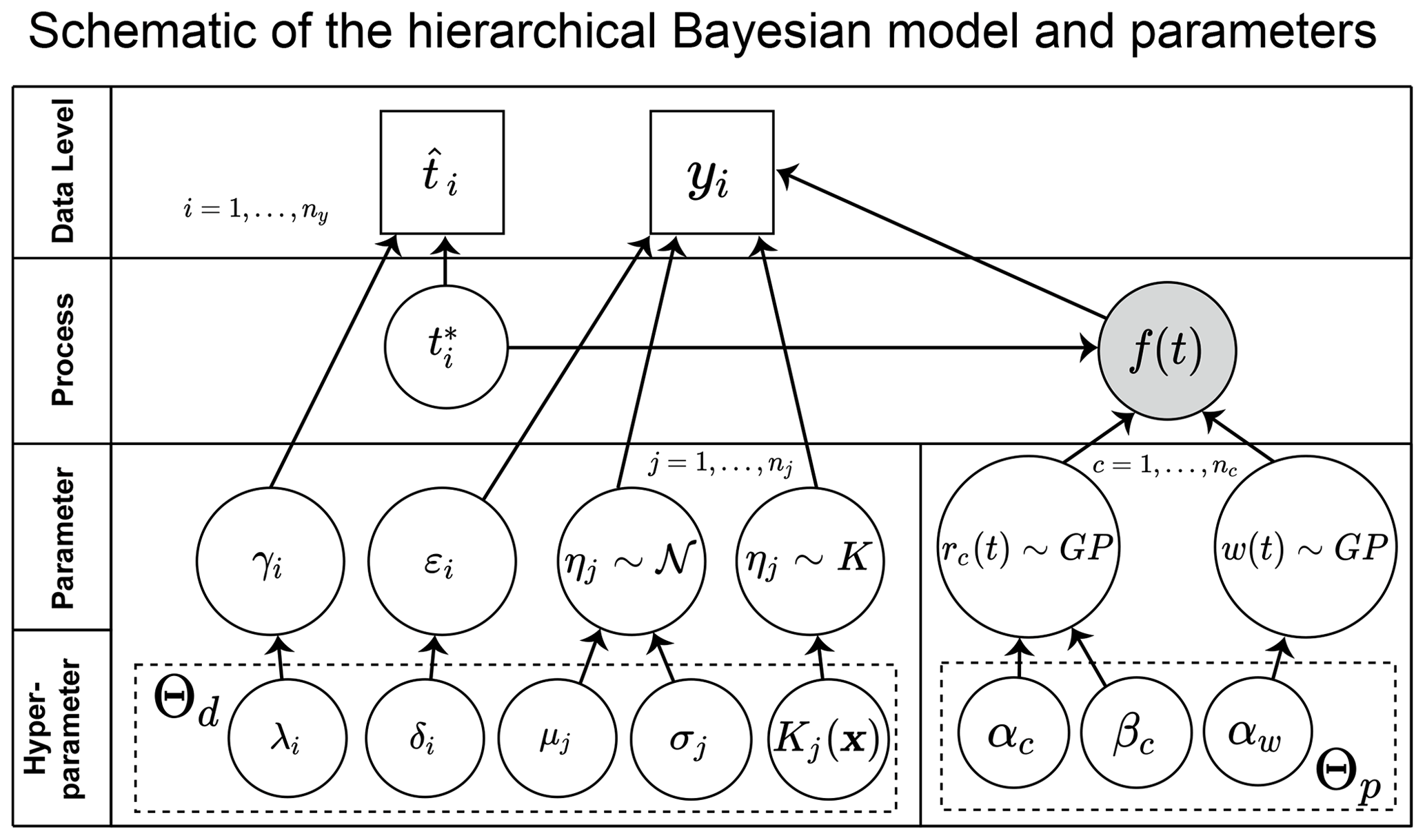
Figure 2Directed acyclic graph of the Bayesian hierarchical framework of our model. Square nodes represent observed quantities (data), and circular nodes represent unknown quantities (latent variables and model parameters), where the gray circle represents the ultimate variable of interest to be modeled. Arrows indicate conditionality. Each node in the graph is conditionally independent of all others, given the parameters in the previous level. Variables and conditional distributions are specified in the main text. The hyperparameters are represented in the lowest level, where x represents the data used in the data-fitting process, and K represents the nonparametric empirical distribution (kernel density function). Parameters of the models in the middle level are controlled by the hyperparameters in the bottom level. The (hyper)parameters on the left (right) represent the data (process) model. Unobserved (latent) variables and f(t) are represented in the process level, such that the data level represents the only observed quantities in the model. Posterior estimates of the parameter distributions contribute to the process uncertainty in the model, and sea levels over time can be estimated from distributions of the data and parameters. The Bayesian nature of the framework allows for the inversion of the conditional distributions resulting in the posterior distribution f(t), the final model output. Further details of each level and the parameters involved may be found in the text.
The goal of our analysis is to determine the probability distribution of RSL through time f(t), based on the observed elevations (y) of proxy data points and their estimated ages . Using hierarchical modeling, we explicitly distinguish between three levels: (1) a data level, (2) a process level, and (3) a parameter level (see Eq. 1). The data model describes , the joint probability for all samples i of each measured elevation yi conditional upon RSL (fi), estimated age (), and the data-level parameters (Θd), multiplied by the probability of an estimated age conditional on the latent (unobserved) true age () and the data-level parameters (Θd). The data level characterizes the way in which RSL is recorded by different proxies through the data parameters, according to modern depth distributions, measurement uncertainties, and dating uncertainties. The process level describes p(f(t)|Θp), the probability distribution of RSL through time f(t) conditional upon the process-level hyperparameters Θp. The parameter level characterizes key attributes (Θp,Θd) of the process and data levels, respectively.
We construct a Bayesian hierarchical model to estimate the posterior distribution of RSL and parameters given observed data.
We follow Parnell et al. (2015) and Cahill et al. (2016) in making some simplifying assumptions and taking a modular approach to implementation of the model (Sect. 2.2). As described in Sect. 2.2.1, we assume that the data model hyperparameters can be estimated from the modern data and that all proxy measurement errors (temporal and elevation) are adequately characterized by the uncertainties defined in the collection of the data. We assume that the relationship between RSL and the elevation of each proxy is independent of the RSL process. We also assume that elevation measurement uncertainty and age uncertainty are independent and normally distributed for all RSL proxies (with both nonparametric and normally distributed likelihoods). Although the assumption of normality in age uncertainty is an oversimplification, many RSL models assume normal uncertainties for calibrated radiocarbon ages or ignore age uncertainty entirely (e.g., Shennan et al., 2002; Engelhart et al., 2009). The widths of the normal versus nonparametric age distributions are also similar (i.e., both capture a similar range of possible ages). In addition, this simplifying assumption both significantly speeds up computation (i.e., O(n3) versus O(n4)) and is unlikely to impact the results of the analysis for the following two reasons: (1) these uncertainties are smaller and have less impact on the posterior distributions of sea level than the uncertainties in the proxy distributions, and (2) the models that we use for comparison in the validation tests also employ the same assumption.
2.1.1 Data level
The data level includes the noisy, observed elevation yi and estimated age of each RSL proxy data point. This level characterizes the relationship between elevation and RSL fi and describes measurement error. We make the simplifying assumptions that the elevation measurement error (ε) and the temporal (age) calibration error (γ) of the RSL proxies are independent and normally distributed, whereas the likelihood distribution (η) with respect to sea level does not need to be parametric, such that
yi,j is the ith observed elevation of the jth proxy type, is the median calibrated age, is the true (unobserved) age, , and . The standard deviations of elevation uncertainty are quantified based on the sampling process, which typically involves sediment coring in contemporary mangrove environments, underwater drilling of coral-reef framework, or extraction of fossil corals from subaerial outcrops. These uncertainties stem from errors inherent in determining the depth of a sample in a core and determining the absolute elevation of a core top or sample within an outcrop relative to a tidal or orthometric datum (Khan et al., 2015; Hijma et al., 2015).
The model can accommodate both parametric and nonparametric fitted distributions as likelihoods (ηj in Eq. 2), which characterize the relationship between elevation and RSL. For corals, a kernel density function (ηj∼K(x)) is fitted to each coral taxa's modern elevation data (x), where j indexes the proxy type, and ηj is a distribution on negative values for coral because their elevations are below MSL (Fig. 1a). See Sect. 2.2.1 for details on the distribution fitting.
Mangrove peats are assumed to form between MTL (mean tide level) and HAT (highest astronomical tide) in a normal distribution with mean μ and standard deviation σ, such that based on the indicative meaning of mangrove peat and local tidal levels (Fig. 1a). This simplifying assumption for mangroves is warranted, both due to analyses of modern mangrove distributions indicating that they are reasonably approximated by a normal distribution (Leong et al., 2018) and due to the relatively small distributional ranges (±1.0 m in South Florida). It is, therefore, worth the computational savings of the assumption of normality. These distributions can also be updated with new data to reflect local distributions. For mangrove peat index points, μj is positive because mangroves are assumed to grow above sea level.
Marine-limiting and terrestrial-limiting data define the lower and upper limits of sea level, respectively. We assume that the RSL likelihood decreases with the distance from the measured elevation of the limiting data. In order for the distribution to be normalized (continuous probability distribution function integrating to 1), we assign these a triangle distribution, which we conservatively bound with a lower (upper) limit of 50 m and an upper (lower) limit of 0 m for terrestrial (marine) limiting data points. In the limiting cases, the distribution of ηj takes the following form:
We maintain the simplifying assumption of conditional independence among observed elevations () and among calculated ages (), although there is clearly a correlation at the process level in the underlying RSL. In other words, we assume the relationship between RSL and the elevation of one observation does not affect that relationship for any other observation. The same is true for age uncertainties. The assumed independence may not strictly hold in all cases (e.g., measurements from the same sediment core where elevation estimates may be correlated). However, most samples in this study are not collected from the same core or are from distinct depositional periods within a core. Furthermore, given the possibility of a sea-level highstand in the circum-Caribbean region, the law of superposition (the geological assumption that sedimentary strata were deposited in ascending order such that the oldest strata will lie at the bottom of the sequence) does not strictly apply. If the elevation estimates were correlated through a single core age model, we would suggest using the law of superposition to inform these estimates.
2.1.2 Process level
In the implementation of the process-level model, we treat RSL f(t) as the sum of several processes with different temporal scales of variability:
where rc(t) represents a nonlinear signal with different parameterizations (which allows for distinct timescales), and w(t) is a white-noise process (which captures high-frequency variability). The rc(t) terms are modeled with mean-zero Gaussian process priors:
where αc is the amplitude (or prior standard deviation), βc is the characteristic timescale for each term, and ρ is a Matérn correlation function with a smoothness parameter of (Rasmussen and Williams, 2006). The choice of smoothness parameter ensures that the signal is “once differentiable” (i.e., it is smooth enough to have a single derivative but not a second derivative) to enable rough changes in RSL rates of change without abrupt changes in RSL. Differentiability is a requirement for the noisy-input Gaussian process (NIGP; see Sect. A1) approach to approximate the effects of geochronological uncertainty. The white-noise term has a standard deviation of αw and captures the high-frequency sea-level variability that is not captured by the other terms.
We choose to employ Gaussian process (GP) priors, which define the relationship among any arbitrary set of points in time (can be extended, without loss of generality, to a higher dimension such as space) as a multivariate normal distribution defined by a mean vector and a covariance matrix. In a GP model, the sea-level function, f(t), is nonparametric (i.e., its form is not predetermined) and can be used to determine trends solely from the data. Accordingly, GP time-series models have much more flexibility than many other models (e.g., temporally linear or change-point models). The shape of the curve is driven by the covariance matrix, which is estimated through the correlations in the RSL data points. While nonparametric, certain conditions or assumptions are inherent in any approach, such as the smoothness or scale of variability, via the type of covariance function or bounds on parameters, for example. Those choices and the hyperparameters of these models are described at the parameter level (Sect. 2.1.3).
2.1.3 Parameter level
At the parameter level, represents the hyperparameters that characterize the process level of the model. Here, , where nc is the number of terms in the model, representing different frequencies; αc represents the prior standard deviations of these nc frequencies of sea-level processes; βc represents the characteristic timescale of variability in sea-level processes; and αw is the prior standard deviation of the white-noise term w(t).
For each parameter, we employ uniform prior distributions with bounds set to separate the terms in the covariance function according to patterns in RSL and to exclude unrealistic interpretations of the data, based on prior knowledge (see Fig. C1 for plots of various hyperparameter combinations). For example, the prior standard deviation (or amplitude) and temporal scale are restricted proportionally, based on the ratio of magnitude to time of RSL change during the Holocene epoch, such that the prior standard deviation parameter α1 may take on values between 5 and 50 m, and the temporal-scale parameter β1 may take on values between 4 and 40 kyr. In contrast the higher-frequency term r2(t) restricts the prior standard deviation, such that α2 may take on values between 0.001 and 20 m, and β2 may take on values between 500 years and 10 kyr. We restrict the bounds on the white-noise standard deviation αw to between 0.001 and 10 m. Prior expectations regarding dominant scales of RSL variability inform our choices of prior distributions on hyperparameters for distinct sea-level processes. For example, glacial isostatic adjustment (GIA; a process driven by the viscous response of the mantle to the changes in ice mass loads since the Last Glacial Maximum) is known to adhere to roughly linear patterns over the past 3 to 4 kyr. Conversely, ocean dynamics occurs on shorter timescales with nonlinear variability (Kopp, 2013). Thus, these processes and others can be decomposed based on various magnitudes and temporal scales. The choices of priors on the hyperparameters allow for variation in this decomposition of terms while adhering to prior knowledge. See Fig. C1 for examples of different hyperparameter combinations.
2.2 Statistical model implementation
We define three modules – a distribution-fitting module, a sampling module, and a sample-wise prediction module – which are implemented in succession. The distribution-fitting module estimates data parameters Θd, which are then used in the sampling module (Eq. 7). The sampling module employs MCMC sampling and accounts for geochronological uncertainty using the noisy-input Gaussian process approximation method of McHutchon and Rasmussen (2011), which translates errors in the independent variable (age) into equivalent uncertainties in the dependent variable (proxy elevation; see Appendix A). The sampling module yields an estimate of (left-hand side of Eq. 7), which is input to the sample-wise prediction module (right-hand side of Eq. 8). The sample-wise prediction module then infers RSL over time (left-hand side of Eq. 8) through the NIGP. Each module is described below.
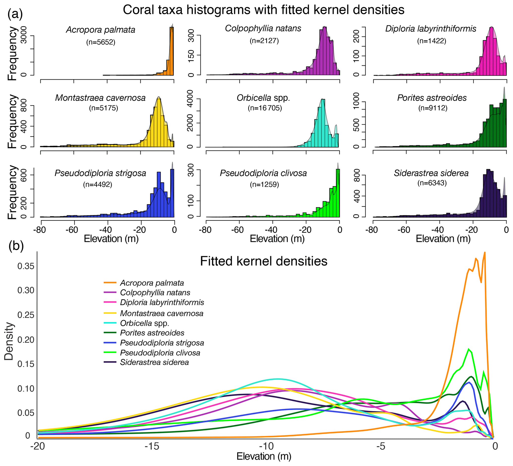
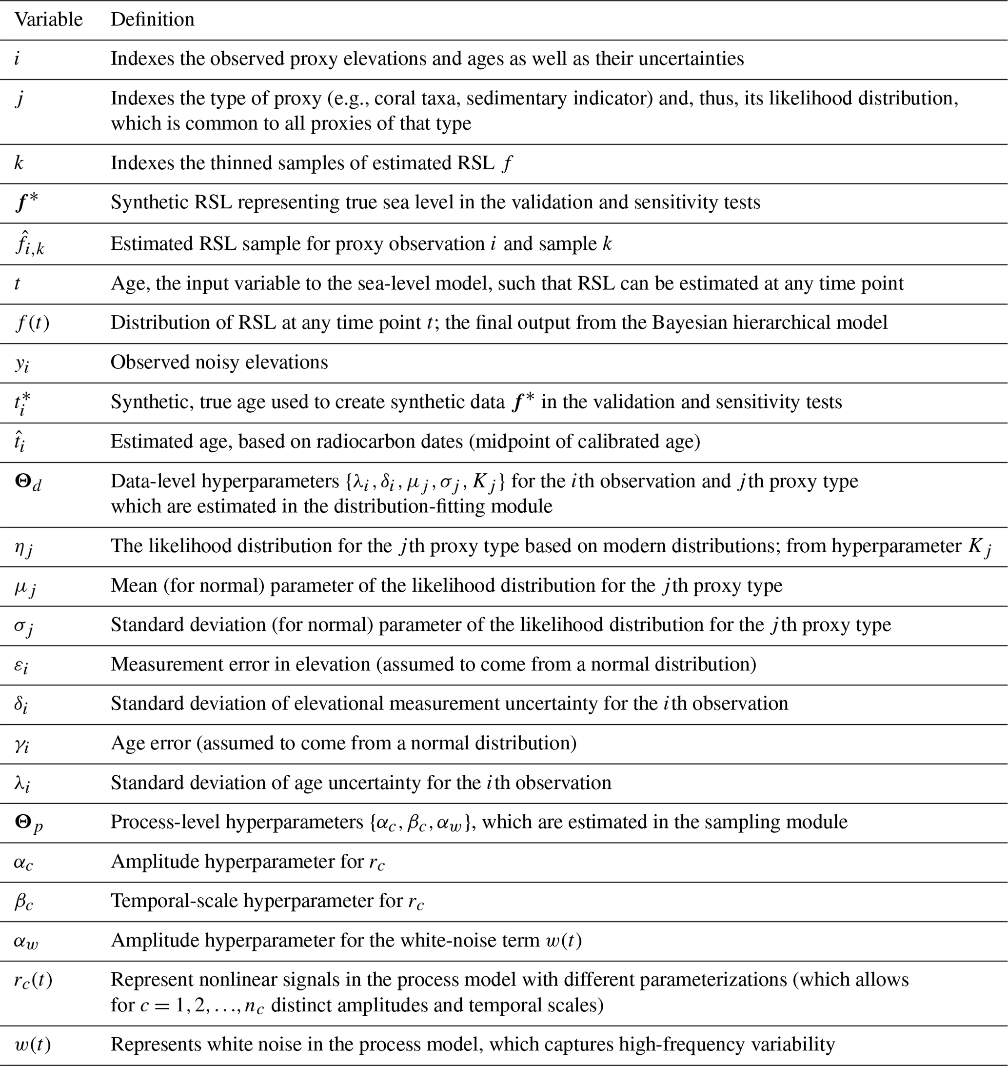
Figure 3Empirical elevation distributions of the nine coral taxa used in the statistical model: (a) histograms of the modern occurrences of the taxa by depth (negative elevation) with kernel densities overlaid (note that frequencies are not on the same scales), and (b) the fitted kernel densities for each taxon on the same scale.
2.2.1 Distribution-fitting module
The distribution-fitting module (Fig. 1b) analyzes the modern proxy elevations in relation to present-day MSL to determine their indicative meanings. Here, we examine the distributions of nine corals (Fig. 3) based on their prevalence in the Quaternary (the past 2.588 million years) fossil record of the western Atlantic/Caribbean region (Pandolfi and Jackson, 2006; Kuffner and Toth, 2017), from which the original RSL proxy datasets are derived. We evaluate observations of modern occurrences of each coral taxa by depth (i.e., elevation of living coral) to determine these distributions, based on data from the ecological studies archived on the Ocean Biodiversity Information System (OBIS) database (OBIS, 2017); see Appendix D, following Hibbert et al. (2016). The majority of the data used in the analysis come from the Atlantic and Gulf Rapid Reef Assessment (AGRRA, 2018). AGRRA monitoring protocols suggest that sampling should focus on reef zones from 1 to 15 m below MSL (−1 to −15 m elevation), which could bias the distribution data; however, the fact that the depth optima of some coral taxa in the database are deeper than 15 m suggests that this bias is small.
We fit nonparametric, empirical probability distributions to the modern coral depth data, using the “fitdist” function in MATLAB (Statistics and Machine Learning Toolbox), to assign the likelihood distribution of each coral taxon for use in the statistical model (Fig. 1b). We use a kernel density with positive support, which restricts the range of RSL to positive values (i.e., elevations of the observed corals are always below MSL). Using a nonparametric approach avoids making assumptions about the distribution of the data (Fig. 3). The kernel smoother assumes that each modern coral elevation has normal measurement uncertainty and assigns an individual probability density curve to each data point. The function has a bandwidth parameter, which can be optimally smoothed. We assigned all taxa densities a bandwidth value of 0.15 m based on (1) the ∼ 1 ft (0.15 m) precision of most underwater depth gauges used to measure coral depths, which is assumed to be the same for all coral taxa, and (2) the central tendency of the optimized bandwidths for all coral taxa (the nine optimized bandwidths have a mean of 0.161 and median of 0.121). In the distribution-fitting exercise, the final probability density function for each coral taxon is the normalized sum of all of the densities of that coral type (for details, see “ksdensity” in the MATLAB statistics toolbox; MATLAB, 2019).
In some cases the nonparametric distributions are bimodal because the depth distributions of corals are controlled both by light, which decreases exponentially with depth, and wave energy, which decreases with depth but is also relatively low in shallow “back reef” lagoon environments behind the wave-breaking reef crest (Hubbard et al., 1988).
2.2.2 Sampling module
In the sampling module (Fig. 1d), we transform the observed paleo-proxy elevations, y, into correlated samples of RSL, , and parameters, Θp, that characterize the sea-level processes. The likelihoods used in the sampling module are the kernel densities for each taxa found in the distribution-fitting module and at the data level (Sect. 2.1.1), such that
Here, n is the number of RSL proxy records in the model; k indexes each set of RSL and process-level parameter samples (nk samples in total); and () represents the vector of RSLs, where subscript −i signifies all points except the ith. Thus, each RSL sample () is successively conditioned on all other current RSL samples and the current GP process-parameter sample p(Θp,k). Temporal uncertainty is again incorporated using the noisy-input Gaussian process (NIGP) method described in Sect. A1. An adaptive Metropolis-within-Gibbs sampling algorithm (Gelman et al., 2011) produces nk thinned samples (). For more details on the algorithm, see Sect. A6.
2.2.3 Sample-wise prediction module
In the sample-wise prediction module (Fig. 1e), we combine each of the nk pairs and Θp,k to get the posterior distribution of RSL over time t:
Each sample Θp,k represents a prior distribution of RSL and is combined with the corresponding RSL sample, , through the NIGP (see Sect. A1 for details). The resulting sample-wise predictive distributions are each () randomly sampled 10 times, resulting in nk×10 total samples of f(t). We then pool these samples to estimate the final posterior distribution of RSL through time. A theoretical illustrative example of the 95 % credible interval and median posterior predictions over time is shown in purple in Fig. 1e.
More precise data have more weight in the model. For example, the less precise Orbicella spp. coral data point at ∼ 5 ka in Fig. 1d and e would alone predict lower RSL; however, because samples are conditioned on all other data, the more precise points of the same age constrain the MCMC samples to the upper limits of the coral likelihood distribution. In contrast, the coral with a relatively low elevation at ∼ 7 ka is the only data point of that age, so the MCMC sampling produces a distribution of samples that broadly matches its original likelihood distribution.
2.3 Validation tests and sensitivity analysis
We performed a model validation of the nonparametric model by comparing its predictions to synthetic “truths” and examined potential improvements over a previous Gaussian model (Khan et al., 2015) and empirical, uncorrelated model (Hibbert et al., 2016). For comparison to the Gaussian model, we also evaluated which portions of potential improvements in the nonparametric model were due to the more realistic interpretation of the data and which were due to including more data in the model. We performed sensitivity analyses by evaluating the performance of the nonparametric model with different quantities and qualities of data.
2.3.1 Model validation
We created five random iterations of a synthetic Holocene RSL dataset to compare model performance to two previously published models. The elevation and temporal uncertainties in the dataset are designed to mimic characteristics of an extensive coral-based Holocene RSL archive from South Florida (Toth et al., 2018a, b; Stathakopoulos et al., 2020; Stathakopoulos and Toth, 2020); reef-derived framework cores are housed at the U.S. Geological Survey core archive in St. Petersburg, Florida (https://doi.org/10.5066/F7319TR3). The South Florida dataset consists of 159 coral samples (Toth et al., 2018b, a) and 62 sedimentary samples (Khan et al., 2017). The 159 coral samples include Orbicella spp. (n=54), A. palmata (n=53), Pseudodiploria strigosa (n=18), Montastraea cavernosa (n=10), Diploria labyrinthiformis (n=9), Colpophyllia natans (n=6), Pseudodiploria clivosa (n=5), Siderastrea siderea (n=3), and Porites astreoides (n=1).
The synthetic “true” RSL curve was created from the ICE-6G_C VM5a GIA model pairing of Peltier et al. (2015). We employed linear interpolation on the GIA values, provided at kiloyear intervals from 11 ka to present, to assign true RSL through time. After generating true ages and RSL at each age, we perturbed those values to generate a dataset that mimics the uncertainties in the real Caribbean dataset. First, we perturbed the true ages, adding random normal error to each based on
where t is true age, is noisy age, γ is age error drawn from a normal distribution ( years), and λ is the standard deviation drawn from a normal distribution with a minimum value of 11 years (λi∼ min(11, 𝒩(140,752)) years). This choice was informed by the age uncertainties from the dataset described above.
We perturbed the true RSL heights with measurement error and to reflect the distribution (indicative meaning) of the indicator elevation relative to RSL:
Here, f* is true RSL, ε is measurement error drawn from a normal distribution ( m), and δ is the standard deviation drawn from a normal distribution with a minimum value of 0.1 m (δi∼ min(0.1, 𝒩(0.55,0.222)) m), also based on the dataset described above. For coral index points, ηi,j is drawn from the jth kernel density for the ith proxy index point (see Fig. 3).
We ran the new nonparametric model, a Gaussian model, and an “uncorrelated model” using the synthetic data described above. The Gaussian model samples hyperparameters instead of using single maximum-likelihood point estimates and can only handle data with normal distributions (i.e., the only coral taxa included is A. palmata, and it is assigned a normal distribution), similar to the implementation in Khan et al. (2017) (see Sect. B2 for full model specification). The uncorrelated model uses MCMC sampling of kernel densities based on the empirical coral depth distributions to predict RSL at ages where there are data, but it does not assume any correlation in time to make predictions elsewhere, similar to the implementation in Hibbert et al. (2016) (see Sect. B1 for details). We analyzed the log likelihoods, the precision of predictions, errors, and bias of each model based on the difference between the predicted median RSL (fi) and true RSL (si) at each time point at which data were generated. The precision is measured by credible intervals (95 % and 67 %), the bias is measured by mean error and median error (med(fi−si)), whereas overall error (or accuracy) is measured by root-mean-square error (RMSE; . We also calculated the total log likelihood of each model, by computing the probability of true RSL within the predicted posterior distribution of RSL at each data point. Another measure to validate the model is the coverage ratio, or the ratio of true RSL (si) within the 95 % (67 %) credible intervals (CIs) to the total number of data points; this ratio should be ∼ 0.95 (∼ 0.67) in a robust model. We compared the validation results using five randomly generated synthetic datasets, identical for the three models: nonparametric, Gaussian, and uncorrelated.
We ran additional validation tests comparing the performance of the nonparametric and Gaussian models to determine which portions of potential improvements were due to the more realistic interpretation of the data using kernel densities and which were due to including more data in the model. In these tests, we approximate both A. palmata and Orbicella spp. data with a normal distribution for use in the Gaussian model so as to compare the models with identical data. We used synthetic time-series data of various precision and quantity in each of 12 scenarios (i.e., runs 1–12 in Table D1). See Sect. 3.1 for results.
2.3.2 Sensitivity analysis
The sensitivity analysis tested the performance of the new model framework using different combinations of synthetic time-series data of various precision and quantity (Table D1). We constructed two synthetic RSL time series that approximate the rates of RSL change observed during the best constrained and most recent interglacial and deglacial periods: (1) the Holocene and (2) the late Pleistocene deglaciation following the Last Glacial Maximum ∼ 21 ka. The first synthetic RSL time series, “SL1” (Fig. 4a), uses a sine curve to simulate rates of change representative of the Holocene epoch, ranging from ∼ −10 to ∼ +10 m kyr−1. The second synthetic RSL time series, “SL2” (Fig. 4a), contains abrupt changes, breaking the model assumption of a smooth true RSL curve with a piecewise linear function. SL2 simulates meltwater pulses (MWPs) that occurred during deglaciation with rates of change potentially up to ∼ 40 m kyr−1 (e.g., Rohling et al., 2008; Lambeck et al., 2014; Abdul et al., 2016). Both time series extend over 12 kyr time periods but are not meant to correspond temporally to real-world changes in RSL.
To test the sensitivity of the model to different types of data, we applied the model to a total of 48 synthetic datasets for each of the two RSL time series. These 48 datasets represent all possible combinations of three factors: (1) the number of data points per 1 kyr period (1, 5, or 10), (2) the precision of the data (combinations of normally distributed sedimentary data, limiting data, and fitted kernel distributions for the two most common coral taxa: A. palmata and Orbicella spp.), and (3) the age uncertainty (normal with a standard deviation of 75 or 250 years). The precision (the inverse of the variance) of each distribution is presented in Fig. 4b, and the factors used in each individual test are provided in Table D1. The synthetic data for the sensitivity tests are generated in the same way as in the model validation (Sect. 2.3.1), except that the true ages are drawn from a uniform distribution within 2 kyr periods during the 12 kyr time period (e.g., ti∼U(4, 2 ka)) and the temporal error has a standard deviation of either 75 years or 250 years.
Figure 4(a) Synthetic relative sea-level (RSL) time series, which simulate rates characteristic of the Holocene (SL1) and the last deglaciation (SL2); (b) precision and elevation of the synthetic data distributions, where sedimentary indicators are normally distributed and centered above mean sea level (MSL), while Acropora palmata (A. palmata) and Orbicella spp. are distributed according to their regional empirical distributions below MSL.
We applied the nonparametric model to the synthetic data, taking 20 000 MCMC samples for each of the 48 tests for each sea-level scenario (SL1 and SL2). We ran each set of tests with five starting seeds (random numbers for replication) in order to maximize randomness and increase sample size for accurate statistical evaluation of the models. Each model run produced a posterior predictive distribution of RSL and its rates of change at 100-year intervals in addition to summary statistics (e.g., 67 % and 95 % credible intervals and coverage, cross-model mean RSL, and root-mean-square errors; Sect. 3.2), which describe the precision and accuracy of predicted RSL relative to true RSL. In addition, we evaluated the ability of the model to successfully predict the maximum rate in SL2 for each iteration of the model, which tests the model's ability to detect MWPs and their timing; therefore, we calculated the maximum median rate predicted from each test to determine the model's success in this capacity for each combination of data.
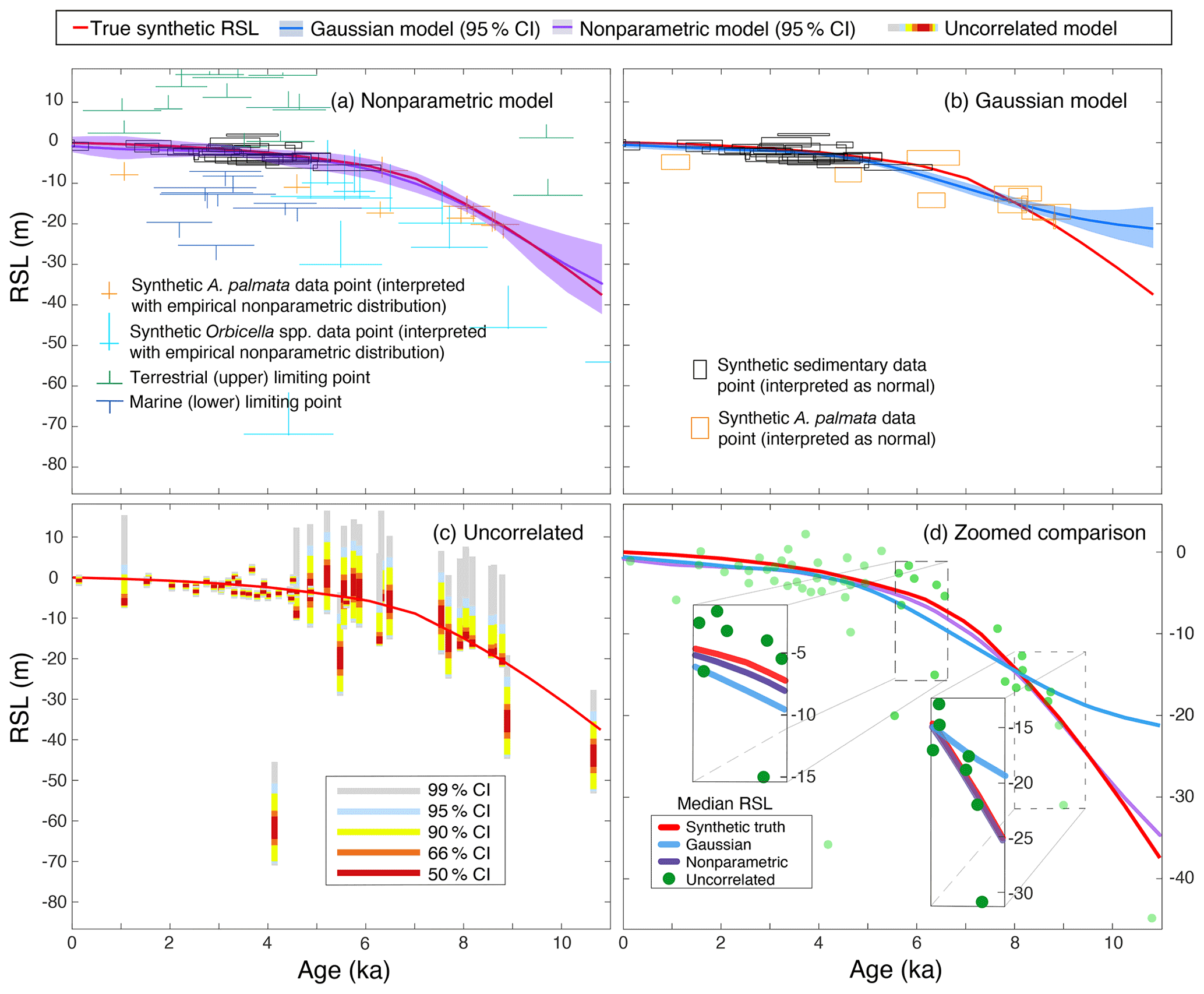
Figure 5Results of validation tests. Comparison of three models using a synthetic dataset based on the modern distributions of Acropora palmata (A. palmata) and Orbicella spp., with median relative sea-level (RSL) estimate and 95 % credible intervals: (a) the current nonparametric model incorporates all available data; (b) the Gaussian model uses the same interpretations of data as in Khan et al. (2017) but samples to incorporate distributions on parameters; (c) the uncorrelated model, similar to Hibbert et al. (2016), uses sampling to infer the probability of RSL at specific times based on modern empirical distributions but without consideration of correlations in time; and (d) predictions from all three models in a single overlapping plot with insets showing model predictions.
3.1 Validation test results
We evaluated the ability of the nonparametric, Gaussian, and uncorrelated models to predict RSL at each point where we generated synthetic data. The log likelihood, credible intervals (CIs), average bias, absolute mean error, root-mean-square error (RMSE), and the coverage of each of the CIs for each model are provided in Table D2. Overall, the nonparametric model performed better than previously published models (both Gaussian, Khan et al., 2015, and uncorrelated, Hibbert et al., 2016) because it incorporates more data than the Gaussian model and uses correlations in time to make predictions where there are no data and the uncorrelated model cannot (Fig. 5). The nonparametric model had a higher likelihood (smaller magnitudes indicate better model fit) across all random seeds with a cross-model mean log likelihood of ∼ −649. The Gaussian and uncorrelated models had cross-model means of ∼ −725 and ∼ −131 305, respectively (Table D2; Figs. 5, 6). The nonparametric model produced RSL estimates with similar precision to the Gaussian model, with 95 % CI widths averaging ∼ 0.87 and ∼ 0.85 m, respectively. The uncorrelated model appears to be much more precise; however, these CI widths are unrealistic given that the coverage of the 95 % CI is only 46 %. The nonparametric model has coverage that is approximately as expected with a cross-model mean of 95.2 % coverage, and the Gaussian model averaged 84.4 % (i.e., less than the expected 95 % of true values fall within 95 % CIs). The 67 % CI coverage results (Table D2) are even more distinct in the different models with cross-model means of 84.0 %, 48.3 %, and 32.0 %, respectively, indicating that the nonparametric model estimates higher-than-necessary uncertainties (CIs are too wide), whereas the other two models produce the opposite result. In other words, the Gaussian and uncorrelated models are overly confident in their predictions at the 67 % CI level, whereas the nonparametric model more conservatively predicts uncertainties.
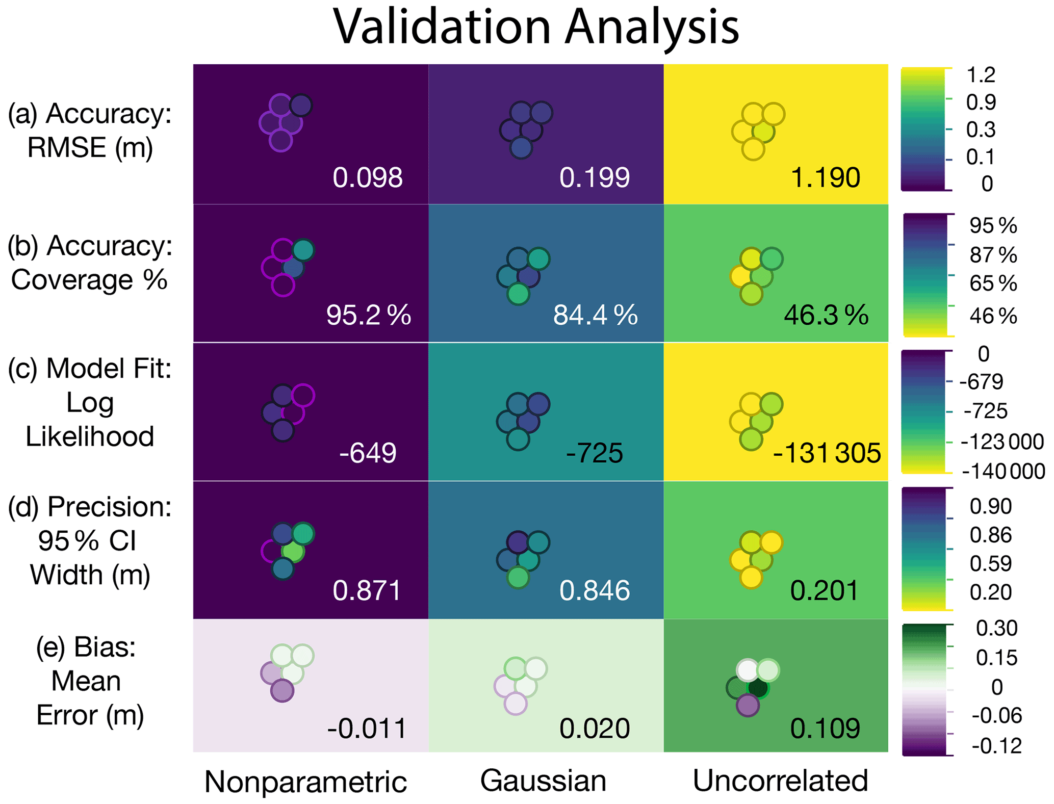
Figure 6Validation test results. These metrics are used to validate the new nonparametric model against the Gaussian and uncorrelated models when applied to equivalent synthetic datasets: (a) accuracy is represented by the root-mean-square error (RMSE); (b) coverage percentage represents the accuracy of uncertainty predictions or the ratio of true synthetic relative sea level (RSL) falling within the predicted 95 % credible interval (CI); (c) model fit is represented by the total log likelihood of each model; (d) precision is represented using the width of the 95 % CI; and (e) bias is represented using the average mean error. Purple (green/yellow) colors indicate better (worse) model performance. The cross-model averages of each metric are shown in each box, and the five runs (for randomness) are represented by the circles, with the position of the circle identifying the seed. Details for each validation test are presented in Table D2.
The nonparametric model also had less bias than the previously published models. The nonparametric model tended to slightly underpredict RSL (negative bias measured by the mean error; cross-model means of ∼ −0.01 m), whereas the Gaussian and uncorrelated models tended to overpredict RSL by ∼ 0.02 and ∼ 0.11 m, respectively (Figs. 5b, c, 6). The validation tests suggest that the uncorrelated model can be extremely inaccurate at points where the elevation of the proxy is far from the true RSL with a cross-model average RMSE of 1.19 m (Figs. 5c, 6; Table D2). This inaccuracy is due to the assumed independence of each sample, as the uncorrelated model does not account for temporal correlation in RSL. Both the nonparametric and the Gaussian models had smaller cross-model averages for RMSE values of ∼ 0.10 and ∼ 0.20 m, respectively, indicating higher general accuracy.
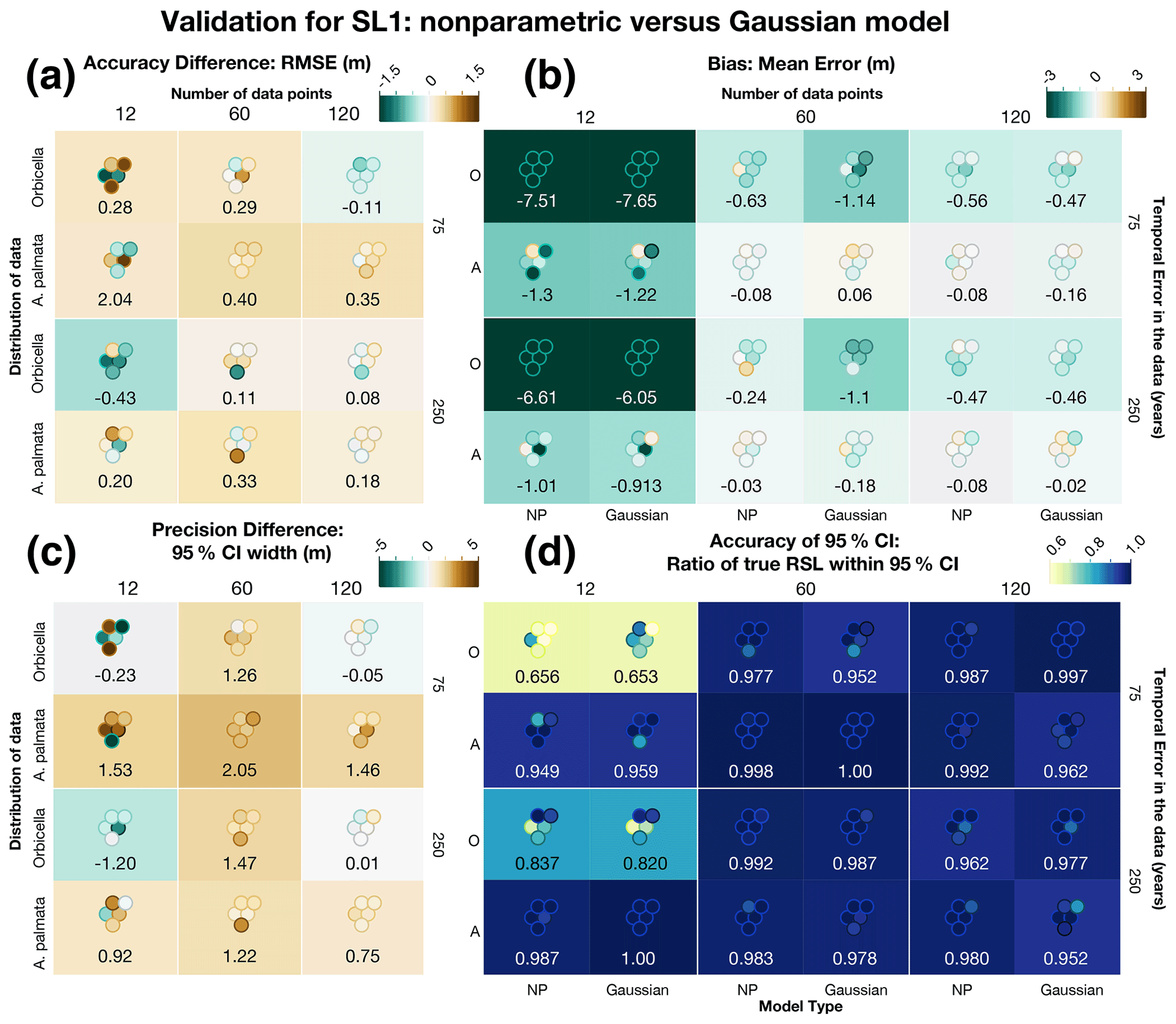
Figure 7Comparison of several metrics to validate the new nonparametric (NP) model against the Gaussian model with the same exact data using sea-level curve SL1. The Gaussian model includes the same quantity of data as the nonparametric model but approximated with normal distributions instead of with kernel densities for both Orbicella spp. (O) and Acropora palmata (A). The differences (a, c) represent the Gaussian metric minus the nonparametric metric. The box colors represent the average metric value (also shown numerically), and each dot represents the individual test, positioned to match the corresponding test run. (a) The difference in the average accuracy of the models, measured by the root-mean-square error (RMSE). (b) Average bias for each model, measured by the mean error, where brown (green) represents positive (negative) bias. (c) The difference in the precision of model predictions, measured by the width of the 95 % credible interval (CI). (a, c) Brown (green) values are positive (negative), signifying that the nonparametric model had less (more) error or more (less) precision. (d) Average accuracy of the uncertainty intervals, measured by the ratio of true values within the 95 % CI. Darker blues represent more coverage (better performance). (b, d) The model type is shown at the bottom of each column. Individual test results for all metrics are shown in Table D3.
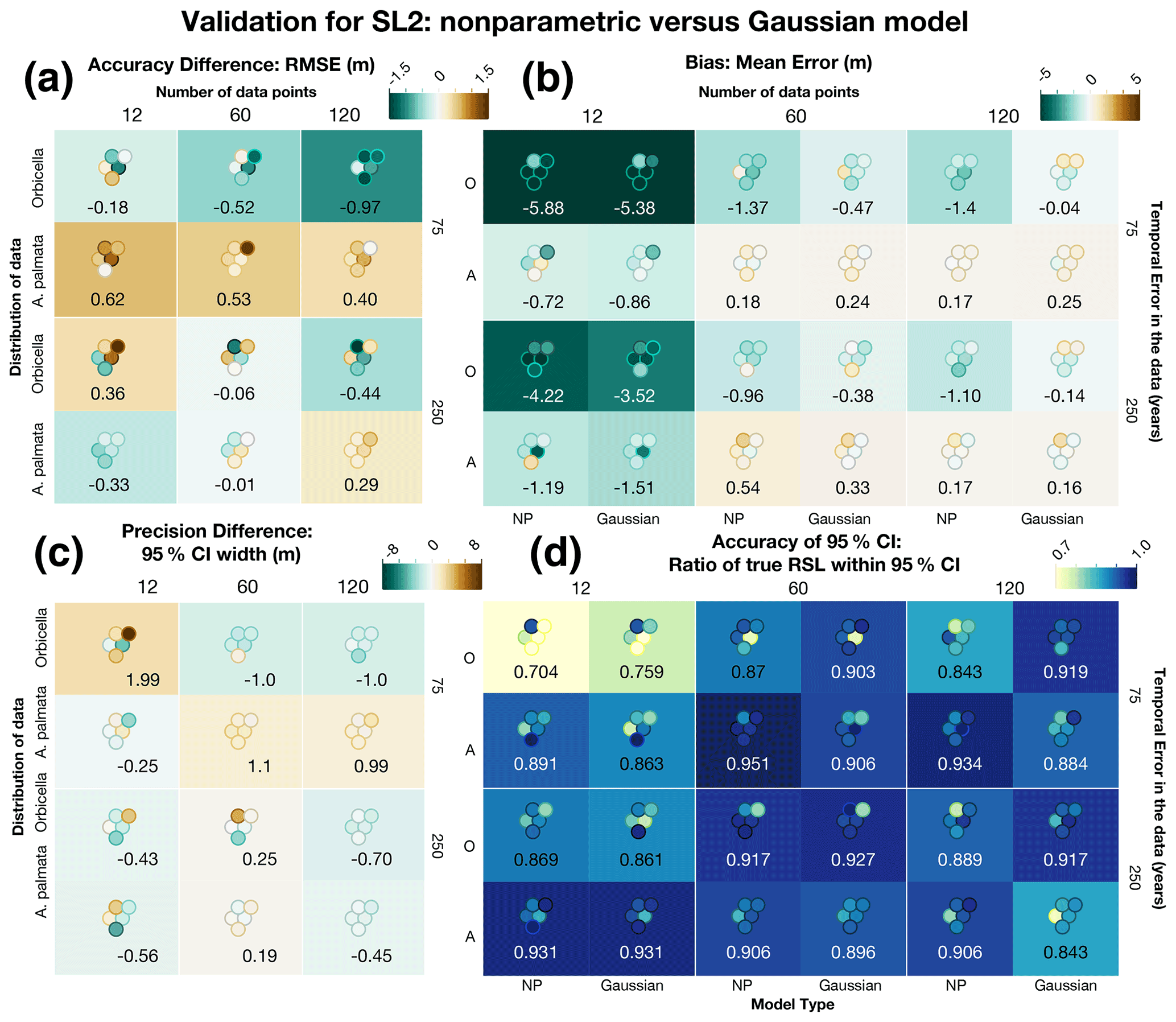
Figure 8Comparison of several metrics to validate the new nonparametric (NP) model against the Gaussian model with the same exact data using sea-level curve SL2. The Gaussian model includes the same quantity of data as the nonparametric model but approximated with normal distributions instead of with kernel densities for both Orbicella spp. (O) and Acropora palmata (A). The differences (a, c) represent the Gaussian metric minus the nonparametric metric. The box colors represent the average metric value (also shown numerically), and each dot represents the individual test, positioned to match the corresponding test run. (a) The difference in the average accuracy of the models, measured by the root-mean-square error (RMSE). (b) Average bias for each model, measured by the mean error, where brown (green) represents positive (negative) bias. (c) The difference in the precision of the model predictions, measured by the width of the 95 % credible interval (CI). (a, c) Brown (green) values are positive (negative), signifying that the nonparametric model had less (more) error or more (less) precision. (d) Average accuracy of the uncertainty intervals, measured by the ratio of true values within the 95 % CI. Darker blues represent more coverage (better performance). (b, d) The model type is shown at the bottom of each column. Individual test results for all metrics are shown in Table D4.
To account for the possibility that the differences in the performance of the nonparametric and Gaussian models were due to the fact that the Gaussian model excludes some (nonparametric) data that the nonparametric model includes, we conducted an additional comparison of the model where the number of data points and uncertainties were equivalent. In 10 of the 12 data cases tested, the nonparametric model had a lower RMSE (Fig. 7a), although the Gaussian model performed better in some cases. The general trend is that models with more data that incorporate A. palmata result in more pronounced accuracy where the nonparametric model performs better. Bias (Fig. 7a) is lower for the nonparametric model in 6 of 12 cases, but the biases are quite similar in those models where the Gaussian model performs better. Conversely, greater bias is more pronounced where the nonparametric model performs better, in particular when using Orbicella spp. data, as would be expected. In 8 of the 12 cases, the precision (Fig. 7b) is higher for the nonparametric model, and the coverage is near equivalent for all models, where each average coverage ratio is greater than the expected 95 % for both models; the only exception is in tests with only 12 Orbicella spp. data points, where the average coverage ratio is less than expected for both models. The results are similar with SL2 (Fig. 8).
These results indicate that the nonparametric model performs slightly better than the Gaussian model when the same amount of data are used in each. Thus, the majority of the improvement stems from the new model's ability to realistically handle nonparametric proxies, allowing the use of more data.
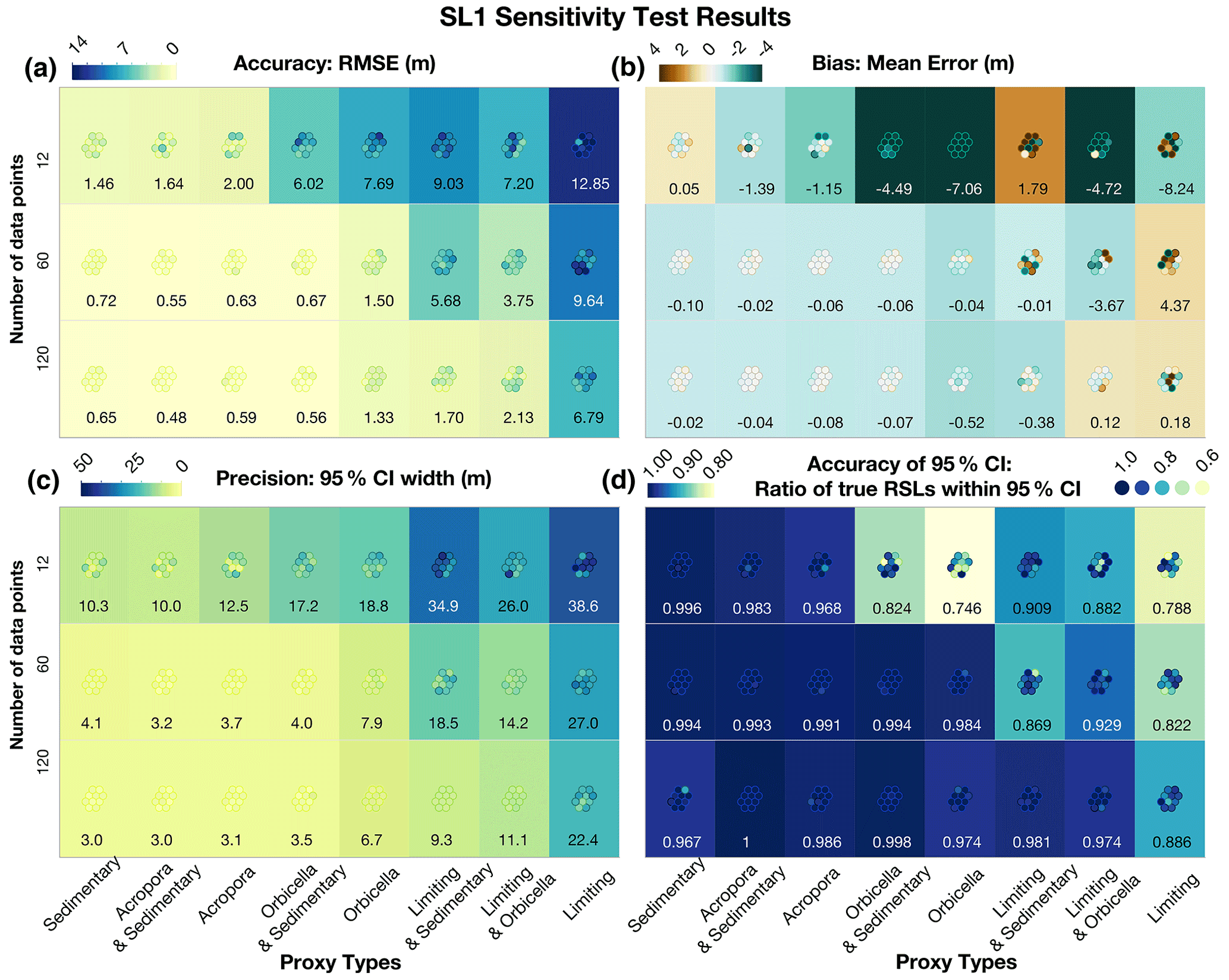
Figure 9SL1 sensitivity test results. The quantity of data is shown on the left, and the type of proxy is displayed on the bottom of each panel. The numbers in the boxes represent the cross-model averages of each metric, and the circles represent each of the individual tests. The specific values of these individual metrics are shown in Table D5. (a) Accuracy is represented by the root-mean-square error (RMSE), where blue values indicate less accuracy; (b) bias is represented by the mean error, where green is negative bias and brown is positive bias; (c) precision is measured by the width of the 95 % credible interval (CI), where blue signifies the least precise model runs; and (d) accuracy of the uncertainty intervals (or coverage %) is measured by the ratio of true values within the 95 % CI, where blue represents the highest coverage or greatest accuracy (Table D5).
3.2 Sensitivity analysis results
The sensitivity tests analyzed how the nonparametric model performs with various amounts and types of data (see Sect. 2.3.2). We compared the true synthetic sea level for each of the two sea-level scenarios to predict median RSL at points every 100 years and calculated CI widths, mean absolute error (MAE), and median error to estimate model precision, accuracy, and bias, respectively (Tables D5, D6). Models that perform well are those that accurately and precisely detect true RSL and rates of change. Consistent with statistical expectations, the sensitivity analyses indicated that the new nonparametric model performs best when the model is applied to high-precision data and/or a higher quantity of data, with trade-offs between the two. Details of the effects of each data factor and results of each test are given in Appendix D. We summarize the overall trends below.
The precision of the data directly affected the precision of the RSL and rate predictions as well as the average error of the predictions for the first sea-level scenario, SL1 (Fig. 9, Table D5). For example, the sensitivity analyses suggested that, in sea-level scenarios similar to the Holocene (last ∼ 12 ka), data that have the precision of sedimentary indicators and/or A. palmata and relatively small temporal uncertainties (standard deviation of ∼ 75 years) were able to constrain rates of RSL change to ±1.8 m kyr−1 at a ∼ 67 % confidence level and ±2.5 m kyr−1 at ∼ 95 % confidence (Table D5).
For tests with low-precision data, uncertainties increased to an average of ±3.0 m kyr−1 at a ∼ 67 % confidence level, and tests with limiting data were unable to constrain rates of RSL change to less than ±6.4 m kyr−1 at 67 % confidence. However, when supplementary sedimentary data were added, tests with limiting data could constrain rates to ± 5.5 m kyr−1 at a ∼ 67 % confidence level. The amount of data also generally affected the precision and the bias of RSL predictions: five per 1 kyr period (versus one point) reduced 95 % CI ranges by an average of ∼ 50 % (Fig. 9c) and cut the bias even more in both cases (Fig. 9c and d, respectively). An increase in the temporal uncertainty of the data from 75 to 250 years affected the models with high-precision data more than the models with lower-precision data but was not the most important factor in performance (Table D5).
The largest factor in the accuracy, precision, and bias of all models was the number of data points (Fig. 9), where including only one point per 1 kyr period (12 total data points) decreased accuracy to an average RMSE of almost 13 m for limiting data only and ∼ 1.5 m for sedimentary data. Precision ranged from a 95 % CI width of ∼ 10–40 m, and bias averaged more than ∼ 0.5 m in tests with only one point per kiloyear. The increases in accuracy, bias, and precision from 1 point per kiloyear to 5 points are generally more significant than those from 5 points to 10 points per kiloyear.
For reconstructing RSL with rates observed during the early Holocene (∼ 10 m kyr−1), employing the nonparametric model with more than one point per kiloyear is generally necessary, even with the most precise data. However, accurate (RMSE < 0.6 m) and precise (2σ<2 m) predictions can be made with almost any combination of sedimentary, Acropora, and Orbicella data. In addition, fairly accurate (RMSE < 1.5 m) and unbiased (magnitude of bias < 0.5 m) results can be produced with 60 points of almost any combination of proxies, except for limiting data alone (see Fig. 9a and b, bottom row). Conversely, precision of model estimates only improves when the nonparametric model is employed with high-precision data.
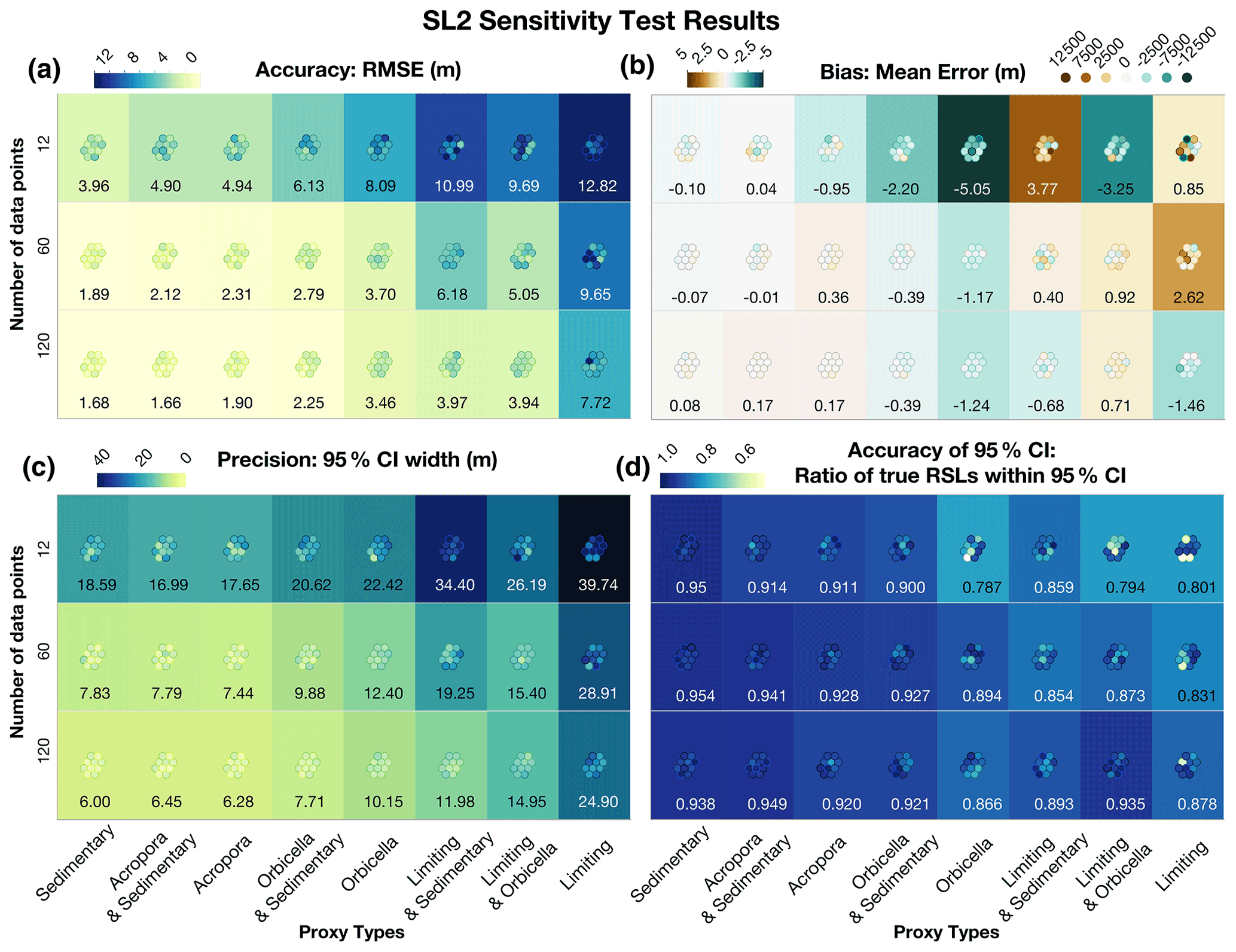
Figure 10SL2 sensitivity test results. The quantity of data is shown on the left, and the type of proxy is displayed on the bottom of each panel. The numbers in the boxes represent the cross-model averages of each metric, and the circles represent each of the individual tests. The specific values of these individual metrics are shown in Table D6. (a) Accuracy is represented by the root-mean-square error (RMSE), where blue values indicate less accuracy; (b) bias is represented by the mean error, where green is negative bias and brown is positive bias; (c) precision is measured by the width of the 95 % credible interval (CI), where blue signifies the least precise model runs; and (d) accuracy of the uncertainty intervals is measured by the ratio of true values within the 95 % CI or coverage percentage, where blue represents the highest coverage or greatest accuracy (Table D6).
In sensitivity analysis of the second sea-level scenario, SL2, which includes abrupt accelerations, results varied (Fig. 10). We test the sensitivity of SL2 to determine whether statistical models are able constrain large accelerations in sea-level rise accurately and precisely. We found that including more than 1 sedimentary or A. palmata data point per kiloyear (12 points total) with age uncertainties of 75 years produced a cross-model average 67 % CI for rates of RSL change of m kyr−1 and a 67 % CI for RSL of m (Table D6, Fig. 12). The cross-model average rate bias was m kyr−1, and the cross-model average bias for RSL was <0.2 m in these same tests. The precision of estimates generally decreased as the precision of the data decreased, as would be expected. Adding 4 or 9 points of data per 1 kyr period (from 1 point to 5 or 10) decreased the 95 % CI width by an average of 43 %–56 % and the 67 % CI width of rates by about 30 %–40 %. The only models with significant bias (predictions averaging more than 2 m above or below true sea level) were those with Orbicella spp. data or limiting data; however, the model resulted in a very low bias when applied to all other datasets (cross-model average error of all other tests of 0.4 m).
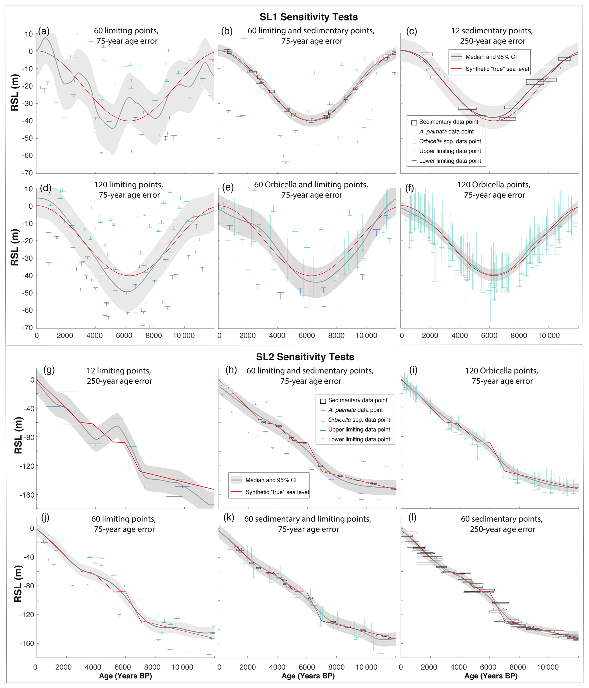
Figure 11Twelve examples of sensitivity tests performed on “true” synthetic relative sea-level (RSL) curves: panels (a)–(e) show sea-level curve 1 (SL1), which represents rates of RSL change similar to the Holocene; panels (g)–(l) show sea-level curve 2 (SL2), which represents abrupt rates of RSL change and maximum rates of up to ∼ 40 m kyr−1, similar to meltwater pulses. For both curves, the red line in each plot represents the synthetic truth. Each of these tests uses various combinations, quantities, and precision of data, which are labeled in each panel.
The sensitivity tests show that high-precision proxies (sedimentary or A. palmata) and dates are important for detecting high rates of change. When data had more precise ages (75-year standard deviation), the model estimated, on average, 2.5 m kyr−1 higher maximum rates (Table D6, Fig. 12), indicating that increasing the precision in dates of indicators can improve model results. However, some models that predict the highest rates of RSL change within the 67 % or 95 % CIs are so imprecise that these predictions mean very little (Fig. 12a, b, c, d). Models with the most bias were those applied with Orbicella data alone or Orbicella in addition to limiting data. In cases where there are sedimentary or A. palmata data to constrain the low-precision data or a greater quantity of data, there was less bias in RSL predictions (Fig. 11b, d, e). However, the bias in RSL did not always affect the ability of the models to predict the rates of abrupt accelerations (e.g., Fig. 12e, f).
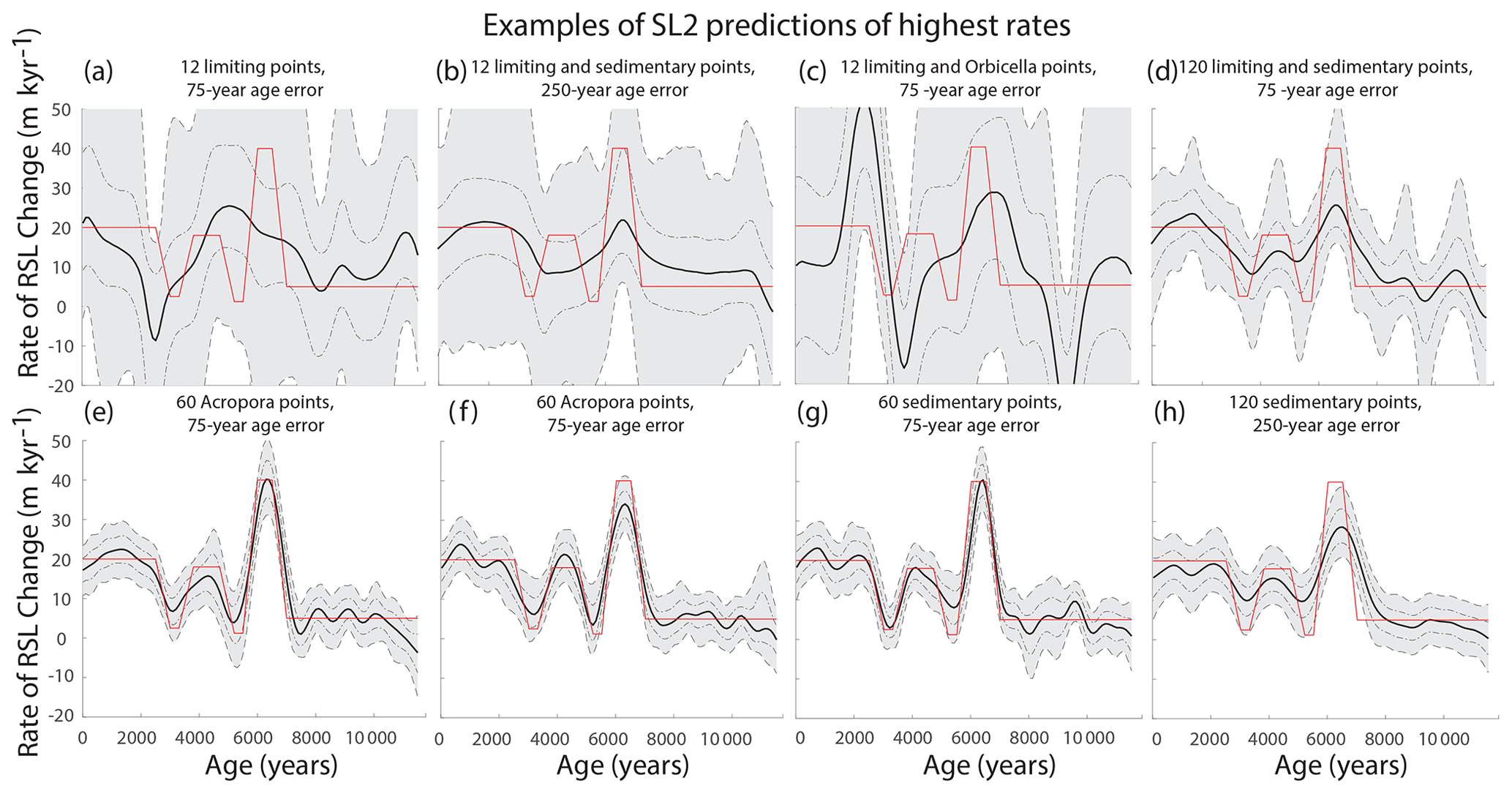
Figure 12Eight examples of sensitivity tests showing various precision and error in rates for sea-level curve 2 (SL2). The red line in each plot shows the true rate, and the black and gray plots show the median and the 67 % and 95 % credible intervals (CIs), respectively. The quantity, precision, and age error of each dataset is labeled above the corresponding plot. Note that panels (e) and (f) have the same data characteristics, but the randomness (i.e., how the data are perturbed for the different seeds) produces different model results.
Tests with different amounts of data varied greatly in their ability to predict true RSL for SL2. For example, Fig. 11g and h display the same type of data (limiting) with different data density, showing that the precision and accuracy increase as the quantity of data increases. It is important to note, however, that including both terrestrial- and marine-limiting data is essential to predictions. In other words, having only lower bounds on sea level would not create accurate results. Data density also influences the ability of the model to accurately constrain sudden accelerations in sea level. For example, the model in Fig. 11g did not predict the timing of sudden changes around 3–4 ka, whereas the model in Fig. 11h did. However, the former predicted the abrupt change at about 7 ka, although with less precision.
The precision of the data also influences model results. For example, the models in Fig. 11i and j, both include the same amount of data. Although the plots appear somewhat similar, the model with more precise Orbicella spp. data (Fig. 11i) produces more precise (95 % CI ± 4.8 versus ± 12.0 m) and accurate (RMSE of 3.5 versus 8.1 m) results. Interestingly, applying the model to data with the same characteristics can result in different model performance. For example, the models in Fig. 12e and f have the same type, amount, and precision of data with the only difference being the random perturbation of the data; however, the model in Fig. 12e predicts rates with more precision and accuracy, whereas the model in Fig. 12f is unable to predict those highest rates with any degree of precision.
In general, all of the models result in a smoothing effect, but a large amount of the most precise data are required to detect abrupt rates of change like MWPs. We find that employing the model with 5 to 10 high-precision data points per kiloyear enables the constraint of rapid rates of RSL (like those represented in SL2) to within m kyr−1 with 67 % confidence.
We develop a new technique for integrating nonparametric likelihoods into a hierarchical statistical framework to allow for a more realistic treatment of proxy uncertainties in probabilistic models of past RSL change. It is more flexible than past methods, with the ability to employ parametric, nonparametric, and limiting distributions. The framework provides a robust method for incorporating fitted empirical elevation distributions of a variety of proxies into RSL models, which we have illustrated with coral taxa.
Validation tests of the new framework show that it performed better than previous (Gaussian and uncorrelated) models based on model fit, accuracy, precision, bias, and overall error, although some of the differences in the model results were small (Fig. 5). Compared with Gaussian and uncorrelated models, the new nonparametric framework had higher likelihoods in all cases, achieved smaller errors (average RMSE of 0.1, 0.2, and 1.3 m, respectively), and had less bias (−0.01, −0.02, and 0.11 m, respectively; Fig. 5) for three reasons. First, assuming Gaussian distributions for RSL proxies when the modern elevations of those proxies are poorly approximated by a Gaussian distribution resulted in less accurate predictions of RSL and poorer model fit than when the kernel densities were applied. Second, employing a model that can handle nonparametric distributions enables the use of more data as input. Third, applying models that do not take advantage of known temporal correlations in sea level (i.e., the uncorrelated model) prevented any statistical prediction of RSL for times with no data and biased RSL predictions when the data fell into the lower-likelihood areas of the kernel densities of low-precision corals (Tables D5, D6).
Although the new model outperformed the previous models when applied to time-series data, its utility for large spatiotemporal datasets may be limited. The flexible, new framework can be adapted to spatial datasets and uses geographic correlations among data, but the computational expense of running fully Bayesian models may be time-prohibitive with large amounts of data ( points). For example, the time to invert a covariance matrix in a GP model scales with the cube of the number of data points, which also prevents the Gaussian model from running with data points. Improvements in high-performance computing, parallelizing code, and more advanced estimation methods for covariances may lessen the differences in implementation times in the future (Ashe et al., 2019). State-of-the art MCMC sampling strategies from off-the-shelf tools in many programming languages (e.g., R, Python) have the potential to make the nonparametric model more useful even with large amounts data. There are also several approximation and estimation techniques, which could speed up performance, that have not yet been applied in a sea-level context, such as variational inference (Blei et al., 2017). We find minimal gains over the Gaussian model when many precise proxies (sedimentary and A. palmata) are included in model runs; therefore, we generally recommend using the Gaussian model for the analysis of larger datasets for which precise data are available.
The quantity, precision, and temporal resolution of the data used in the model were important factors in the accuracy and precision of RSL reconstructions in validation experiments and sensitivity tests. Although including some data (5 or 10 points per kiloyear – 60 or 120 points total) with high precision assisted in creating the most accurate models of RSL change, there was generally a trade-off between the quality (precision or uncertainty) and quantity of data. Using the most data possible, from a variety of RSL proxies with well-characterized likelihood distributions, provided the most accurate and precise estimates of past RSL variability as shown in sensitivity tests (Tables D5, D6). These results could be used by researchers to optimize sampling strategies by providing a priori targets of sample densities and types based on the precision needed for reconstructing sea level for a particular time period and locality.
Our results also have implications for how low-precision data should be interpreted and used in the new framework. We found that models that used precise, sedimentary data and the low-precision kernel distributions of Orbicella spp. tended to produce more accurate and precise results than models using sedimentary and limiting data. Thus, it is better to have known fitted distributions to interpret data, rather than using terrestrial- or marine-limiting bounds. Moreover, when incorporating low-precision, massive coral data (Orbicella spp.) into the new framework, efforts should also be made, if possible, to refine the empirical distributions by further evaluating characteristics of their depositional environment and the taphonomy and morphology of the coral samples (e.g., Stathakopoulos et al., 2020; Blanchon and Perry, 2004; Perry and Hepburn, 2008) to increase their precision and improve model performance. The depth distributions of corals also have the potential to vary by location (Hibbert et al., 2018), so the empirical distributions could be further refined in areas where location-specific modern data are available. Therefore, we recommend using empirical distributions when no other information (e.g., reef facies or epibionts indicative of shallow-water environments to refine coral indicative meaning) or no additional, more precise data (e.g., sedimentary or A. palmata) are available at a location or for a time period of interest.
The new framework developed in this study has broad applicability to the analysis of past RSL. Many previous studies do not appropriately incorporate data uncertainties nor do they estimate rates in a statistically robust way. As discussed above, the flexibility of the new framework enables integration of proxies previously unused in Gaussian models (e.g., massive corals, limiting data). This provides an important improvement over previous RSL models, particularly in places or for periods of time where sedimentary indicators may not accumulate or preserve (e.g., Woodroffe et al., 2015). In addition, the new framework could be applied to assess rates of change during MWPs recorded in deglacial datasets. For example, while Deschamps et al. (2012) relied primarily on a handful of corals with narrower and shallow paleowater depth estimates to define the timing and magnitude of MWP-1A (between 13 500 and 14 700 years ago), inclusion of all of the coral data across this interval – even those with larger paleowater depth ranges – may help to better constrain the MWP according to our assessment of the model performance. Although the new framework produced some biased RSL height results compared with true RSL in sensitivity tests, the estimated rates of RSL change were less biased, even in sea-level scenarios with high rates of sea-level rise (∼ 40 m kyr−1). Average errors in the rates of RSL change were reduced by one-half when a sufficient amount of data (> five points per kiloyear) were included (∼ 0.3 m kyr−1 versus ∼ 0.6 m kyr−1). In fact, the synthetic tests performed in this study may call the validity of previously estimated rates of change during deglacial periods or MWPs into question, as the sensitivity tests have shown that more data are necessary to accurately and precisely constrain rates, even in the new nonparametric model. The new framework may also be used to evaluate the timing and magnitude of sea-level highstands in Holocene and Last Interglacial records. For example, the amplitude of highstands inferred in previous models (e.g., the Gaussian model used in Khan et al., 2017) may prove inaccurate or be overestimated. Based on results of the validation tests, the Gaussian model can be positively biased by more than 1 m, suggesting that further analyses are required to evaluate highstand timing and magnitudes.
Application of the new framework to sea-level datasets from a variety of locations and time periods has the potential to reveal more precise and accurate estimates of rates of RSL because the new framework has less bias, especially in rates. The nonparametric framework also allows the incorporation of limiting data, which could be valuable when there are long hiatuses of other data. In addition, the framework can statistically incorporate information that refines coral indicative meaning (e.g., by incorporating location-specific proxy depth distributions) that produce nonparametric likelihoods. At a minimum, this new framework could serve as a check on previous results when models similar to the Gaussian and uncorrelated models have been used. Although we have demonstrated the model’s potential using synthetic datasets, the future application of the new framework to real datasets could include previously unincorporated data to better estimate past RSL and rates of RSL change.
A1 Noisy input Gaussian process – NIGP
Age uncertainties are incorporated using the NIGP method of McHutchon and Rasmussen (2011), which uses the first-order Taylor-series approximation (a linear expansion about each input point) to translate errors in the independent variable (time) into equivalent errors in the dependent variable (RSL), such that age error is recast as sea-level error proportional to the squared gradient of the GP posterior mean (McHutchon and Rasmussen, 2011).
where is the sea-level process at time, , γi is the age error, and is the partial derivative of f with respect to . Age uncertainties are assumed to be normally distributed, such that . The approximation of f is
where ε is the normally distributed elevation measurement uncertainty in Sect. 2.1.1, such that (from Eq. 2). The predictive posterior distribution is a GP with mean, , and variance 𝕍[f∗]:
where ε2 is the vector of all , Σt is the age noise matrix, Γ is the matrix of derivatives, M is the original training covariance matrix, M* is the covariance between test t∗ and training points , and is the corrective variance term added to output noise, so that inputs (ages) can be treated as deterministic. See McHutchon and Rasmussen (2011) for more details.
A2 Markov chain Monte Carlo sampling – MCMC
The MCMC samples of and Θp, conditional on y, , and Θd, are generated using a Metropolis-within-Gibbs algorithm based on the following derivation. Assuming all parameters of Θp take a uniform prior distribution, (Eq. 7) can be estimated analytically from the NIGP predictive equations of McHutchon and Rasmussen (2011) (Sect. A1) using as the test point and all other data as the training data. Thus, samples of are created according to the likelihood of each randomly generated by calculating and multiplying and accepting or rejecting proposed samples based on the ratio A:
Here, the numerator represents the likelihood of the newly proposed sample , and the denominator represents the likelihood of the last sample accepted , both conditional on the previously accepted samples for all other variables.
Proposed samples of Θp are equivalently accepted or rejected based on the ratio A′:
where θh represents the hth hyperparameter in Θp.
The whole model is summarized in three modules:
-
Distribution-fitting module. Each coral taxa assumes a fixed modern coral distribution, based on the modern coral elevations with respect to MSL from OBIS or its indicative meanings. These distributions are used as likelihoods in step 2.
-
Sampling module. This step generates samples of RSL () and process hyperparameters (Θp). Inputs comprise y, , Θd, and f(t) (Eqs. 5, 6). The step proceeds by
- a.
initializing and Θp,0 (the vector of sea-level hyperparameters ) and all step sizes;
- b.
sequentially sampling new , based on NIGP predictions and the likelihood, with acceptance probability =A (Eq. A5) and each with acceptance probability (Eq. A6);
- c.
every 40th iteration, step size is reassigned (proposals are randomly sampled from a normal distribution with standard deviation of the initialized or recalculated step size) to optimize acceptance ratio (Gelman et al., 2013) according to two conditions,
- –
if a ratio > 0.3 or count < 5, the step size standard deviation is increased, or
- –
if a ratio < 0.2 is accepted, the step size standard deviation is decreased.
- –
- a.
-
Sample-wise prediction module. This step combines thinned samples of and Θp,k, the samples of RSL, and the process hyperparameters through the NIGP predictive equations of McHutchon and Rasmussen (2011) (Sect. A1). In this step, accepted samples are thinned based on sample autocorrelations. For each sample k, a pair represents a prior GP, conditioned on a set of data, which creates a posterior GP that can be used for predictions. A total of 10 samples of predictions over time are drawn from the thinned sample pairs. All 10 × nk sample predictions are pooled to estimate the final posterior distribution . Each estimate is consistent (and equally likely) given the observed data and data parameters.
B1 Uncorrelated method
The published uncorrelated method samples in both age and elevation measurement uncertainty, whereas the age is assumed to be constant in our approximation of that method. In this way, the log likelihood of the method achieves a higher value than it would if we assumed a bivariate distribution of uncertainties for each data point.
There is no correlation assumed between the data. Instead each nonparametric distribution is directly applied to each indicator, which individually determines the “posterior” probability of RSL at each point.
B2 Gaussian implementation
The Gaussian model is similar to the implementation in Khan et al. (2017). The published method implements a spatially correlated component by adding terms to the process level. These terms employ covariance functions that allow the correlation of data in both time and space to add information from other sites. See Khan et al. (2017) for more details.
We analyzed the results of various combinations of hyperparameters in order to restrict the bounds within the model framework. Figure C1 shows some examples of these combinations. When the ratio between the amplitude and the temporal scale of the covariance function is too high, the model predicts high-frequency wiggles that are unfounded in the known processes that affect relative sea level. When this ratio is too low, the model resorts to the prior distribution (in most cases the zero-mean prior) instead of gaining information from the data. The results of high white-noise amplitudes are wide bounds on all estimates of RSL (Fig. C1a, bottom plot).

Figure C1Examples of various hyperparameter combinations and the way they influence how the same data are interpreted and reflect the predicted relative sea level (RSL).
The average results of the analyses are shown in Tables D5 and D6, and the full results of the individual sensitivity and validation tests are available with the code and data at https://github.com/ericaashe/Nonparametric.
Monte Carlo Markov chains are strongly autocorrelated, which produces clumps of samples that may not be representative of the true underlying posterior distribution. Analyzing these autocorrelation plots leads us to accept every 20th MCMC sample (thinning by discarding the other 19 samples) so that samples are approximately independent of one another (Fig. D1a). We check convergence of a model or parameters in a model by looking at the progression of values. The number of samples to throw out is determined by how long (how many samples) it took for the model to converge. For example, in Fig. D1e, the first ∼ 50–75 samples must be “burned” or thrown out to achieve a representative posterior sample.
Table D1Temporal data density, age uncertainty, and proxy distributions used to create synthetic data to perform the sensitivity tests of the nonparametric model. Runs 1–12 are also applied in the validation tests comparing the nonparametric and Gaussian models (Sect. 2.3.1).
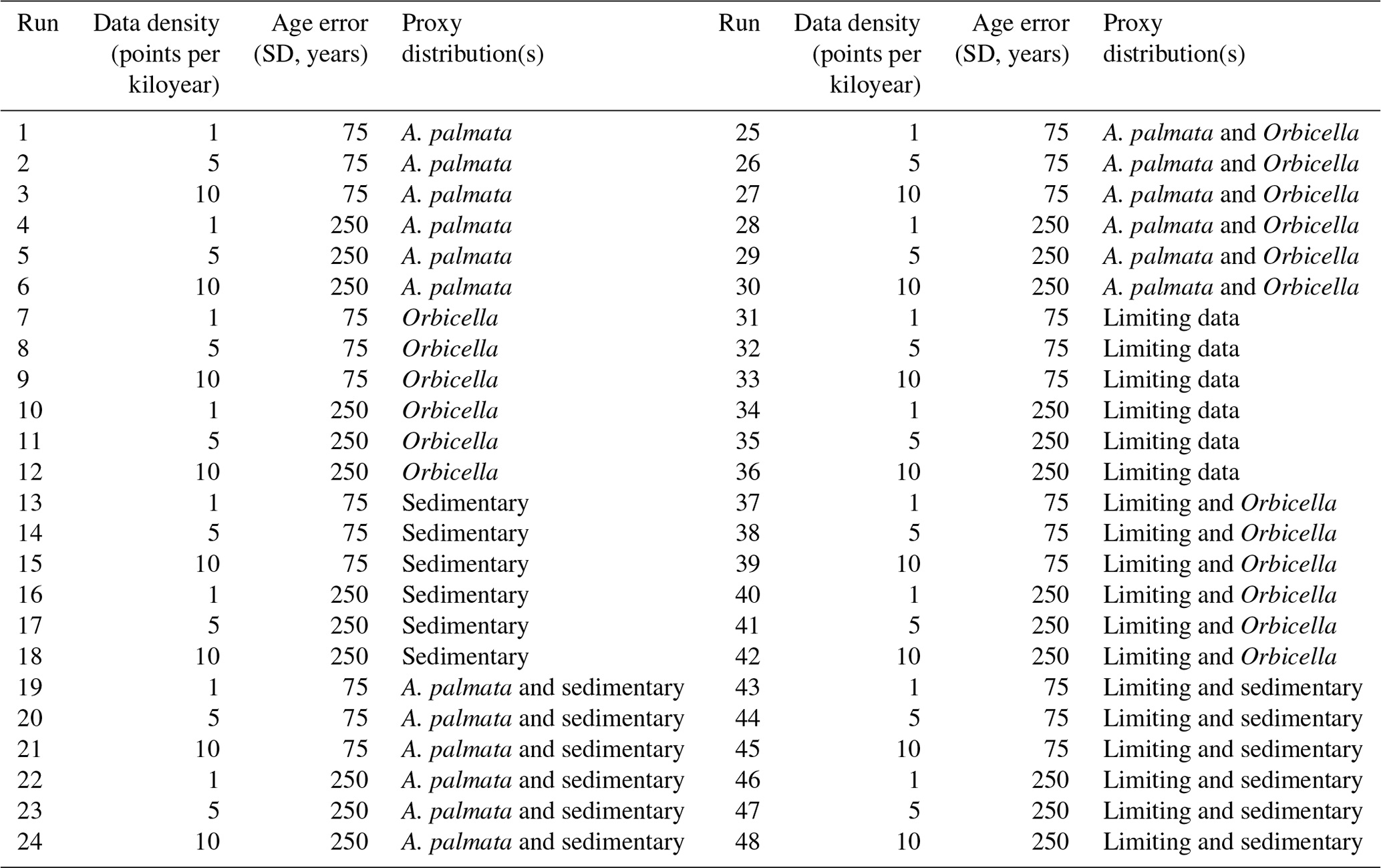
Table D2Validation tests results: model comparison of nonparametric, Gaussian, and uncorrelated models.
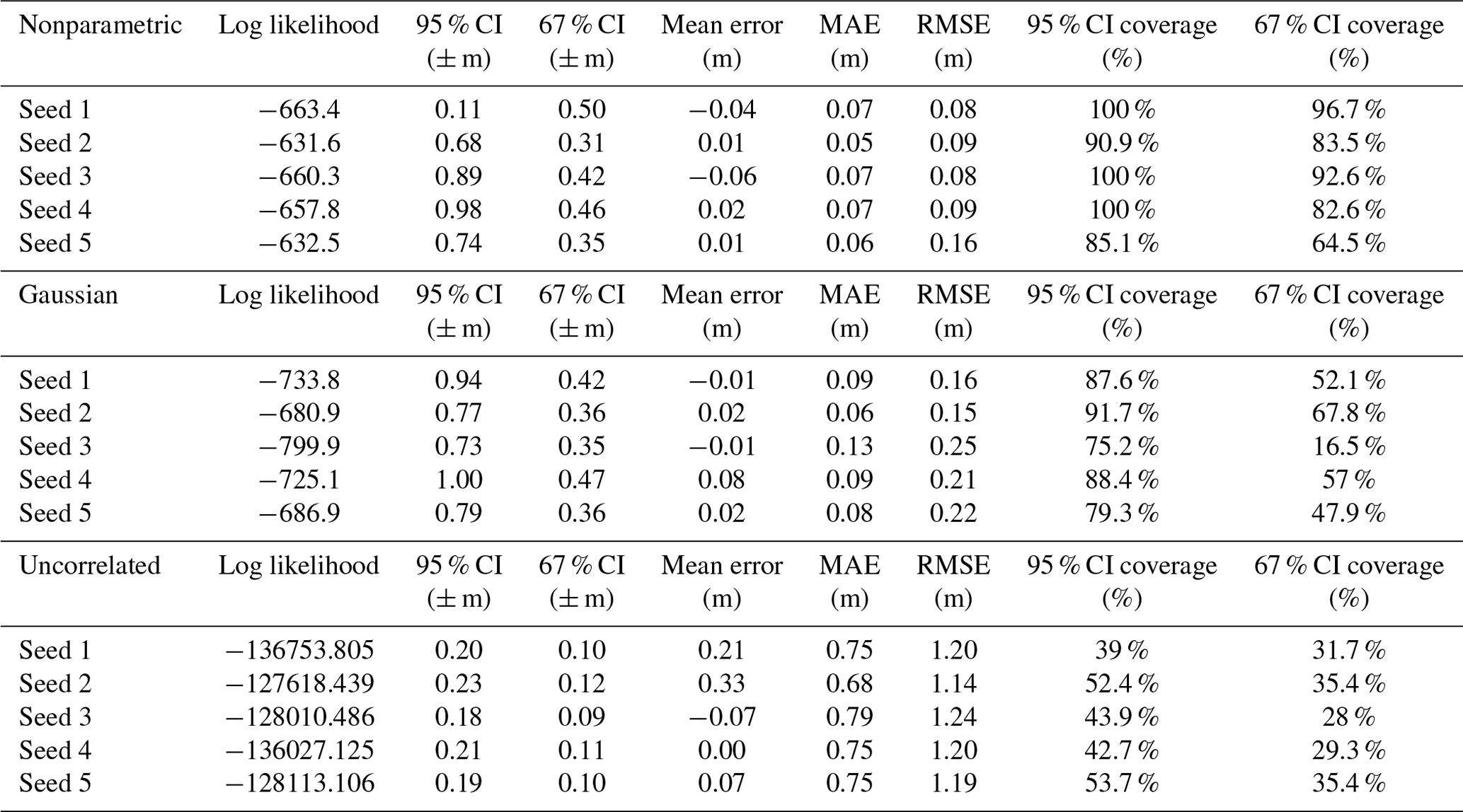
Table D3Summary of validation test results for the Gaussian model, which are compared to the nonparametric model results (Table D5, select test parameters) with same exact data for sea-level scenario 1 (SL1) to determine the portion of improvement from more precise empirical distributions versus the inclusion of more data in the nonparametric model. See Fig. 7 for a visual representation of the comparison.

Table D4Summary of validation test results for the Gaussian model, which are compared to the nonparametric model results (Table D6, select test parameters) with same exact data for sea-level scenario 2 (SL2) to determine the portion of improvement due to the empirical distributions versus due to the inclusion of more data in the nonparametric model. See Fig. 8 for a visual representation of the comparison.

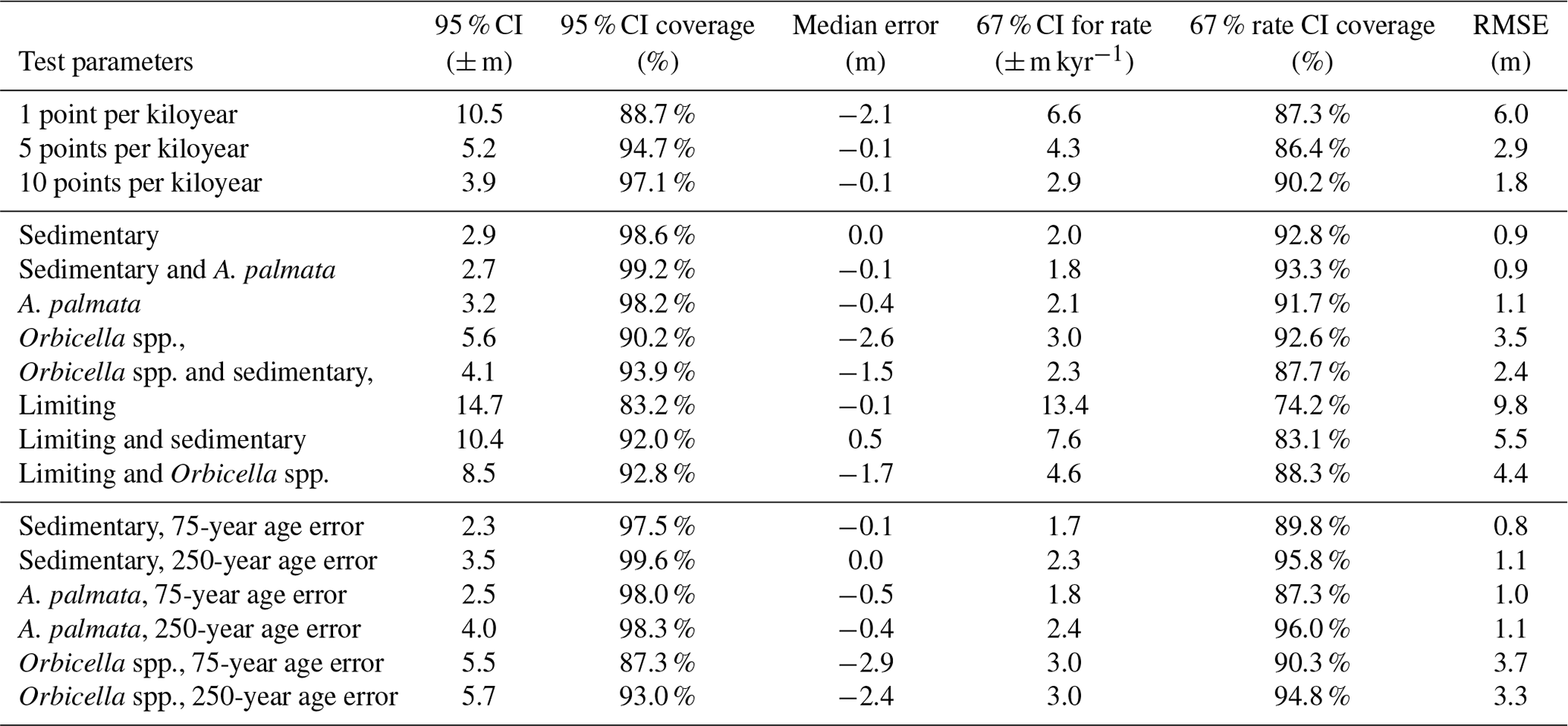
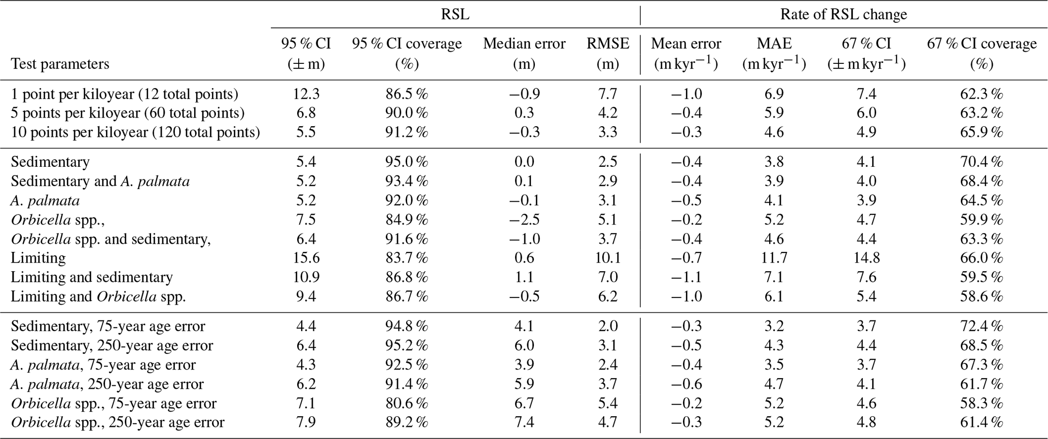
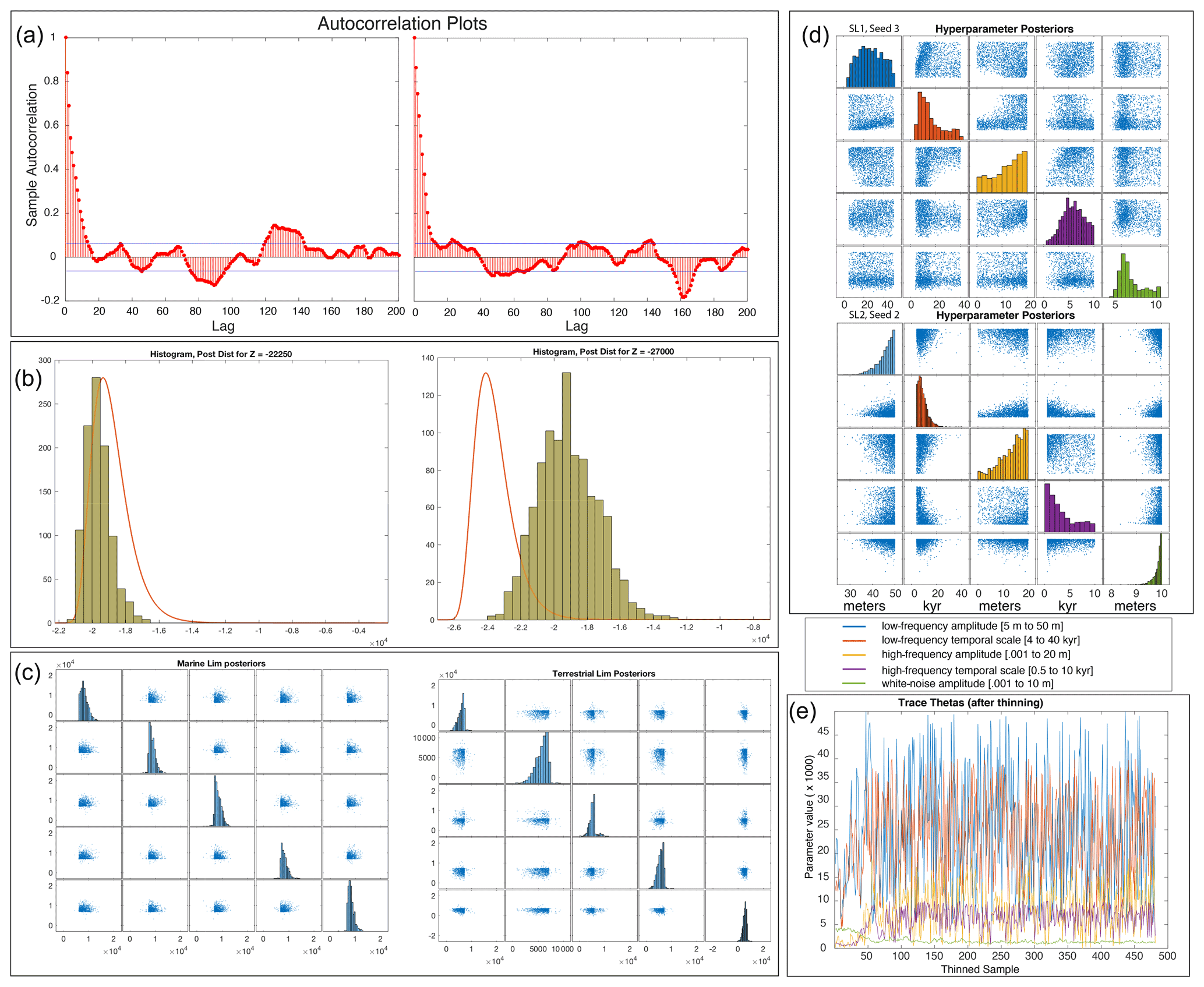
Figure D1Model diagnostics. (a) Autocorrelation plots show the autocorrelation between one sample and the following sample in order to determine the number of samples to discard to result in independent samples of the posterior distribution. (b) Two examples of prior likelihoods of proxy data (red line) and a tan histogram representing the (thinned) posterior sample distribution after going through the sampling module. This posterior distribution of samples (similar to the samples in Fig. 1d and e) may be significantly different from the prior likelihood because of the correlation with other data points that are close in age, such that other data may have influenced the posterior likelihoods. (c) Plots of posterior distributions (diagonal plots) of marine- and terrestrial-limiting data show that the data samples are correlated (off-diagonal plots). (d) Examples of posterior distributions of the hyperparameters of the model for sea-level curve 1 (SL1) and sea-level curve 2 (SL2), where the distributions are colored to match the hyperparameter that they represent, shown in the legend. The bounds on each parameter's uniform prior are also shown in the legend. (e) The trace plot shows the progression of values to check for convergence.
The MATLAB code and data required to run the models can be found on GitHub: https://github.com/ericaashe/Nonparametric (https://zenodo.org/record/5542542, Ashe, 2021).
ELA developed the methodology and models (with help from REK) and designed, implemented, and tested the software and models. REK conceived the project (with help from AD), developed the original base code, and acquired funding. LTT and NSK curated, synthesized, and performed preliminary analysis on the data. All co-authors contributed to writing, reviewing, and editing the manuscript.
The contact author has declared that neither they nor their co-authors have any competing interests.
Any use of trade, firm, or product names is for descriptive purposes only and does not imply endorsement by the U.S. Government.
Publisher's note: Copernicus Publications remains neutral with regard to jurisdictional claims in published maps and institutional affiliations.
Robert E. Kopp and Erica L. Ashe (grant nos. OCE-1831450, OCE-1702587, and OCE-2002437) and Andrea Dutton (grant no. 2041325) were supported by the National Science Foundation. Lauren T. Toth was supported by the U.S. Geological Survey Coastal and Marine Hazards and Resources Program. This work is a contribution to IGCP Project 639 “Sea Level Change from Minutes to Millennia”, INQUA Project CMP1601P “HOLSEA”, and “PALSEA3”.
This research has been supported by the National Science Foundation (grant nos. OCE-1702587 and OCE-2002437).
This paper was edited by Reik Donner and reviewed by three anonymous referees.
Abdul, N. A., Mortlock, R. A., Wright, J. D., and Fairbanks, R. G.: Younger Dryas sea level and meltwater pulse 1B recorded in Barbados reef crest coral Acropora palmata, Paleoceanography, 31, 330–344, https://doi.org/10.1002/2015PA002847, 2016. a
Marks, K. W.: AGRRA Database, version (2018-03), http://www.agrra.org/data-explorer/explore-summary-products/ (last access: 4 Ferbruary 2022), 2018. a
Ashe, E. L.: https://github.com/ericaashe/Nonparametric, Zenodo [data set and code], https://zenodo.org/record/6014827 (last access: 8 February 2022), 2021. a
Ashe, E. L., Cahill, N., Khan, N. S., Kemp, A. C., Engelhart, S. E., Horton, B. P., Parnell, A. C., and Kopp, R. E.: Statistical modeling of rates and trends in sea level, Quaternary Sci. Rev., 204, 58–77, https://doi.org/10.1016/j.quascirev.2018.10.032, 2019. a, b
Blanchon, P. and Perry, C. T.: Taphonomic differentiation of Acropora palmata facies in cores from Campeche Bank Reefs, Gulf of México, Sedimentology, 51, 53–76, https://doi.org/10.1046/j.1365-3091.2003.00610.x, 2004. a
Blei, D. M., Kucukelbir, A., and McAuliffe, J. D.: Variational Inference: A Review for Statisticians, J. Am. Stat. Assoc., 112, 859–877, 2017. a
Cahill, N., Kemp, A. C., Horton, B. P., and Parnell, A. C.: A Bayesian hierarchical model for reconstructing relative sea level: from raw data to rates of change, Clim. Past, 12, 525–542, https://doi.org/10.5194/cp-12-525-2016, 2016. a, b, c, d
Cressie, N. and Wikle, C. K.: Statistics for spatio-temporal data, John Wiley & Sons, Ltd. Sons, ISBN 978-0-471-69274-4, 2015. a
Deschamps, P., Durand, N., Bard, E., Hamelin, B., Camoin, G., Thomas, A. L., Henderson, G. M., Okuno, J., and Yokoyama, Y.: Ice-sheet collapse and sea-level rise at the Bølling warming 14,600 years ago, Nature, 483, 559–564, https://doi.org/10.1038/nature10902, 2012. a
Engelhart, S. E., Horton, B. P., Douglas, B. C., Peltier, W. R., and Törnqvist, T. E.: Spatial variability of late Holocene and 20th century sea-level rise along the Atlantic coast of the United States, Geology, 37, 1115–1118, 2009. a
Gelman, A., Brooks, S., and Jones, G. L., eds.: Handbook of Markov Chain Monte Carlo, Chapman & Hall/CRC Press, ISBN 978-1420079418, 2011. a
Gelman, A., Carlin, J. B., Stern, H. S., Dunson, D. B., Vehtari, A., and Rubin, D. B.: Bayesian Data Analysis, Chapman & Hall/CRC Press, London, 3rd Edn., ISBN 978-1439840955, 2013. a
Hay, C. C., Morrow, E., Kopp, R. E., and Mitrovica, J. X.: Probabilistic reanalysis of twentieth-century sea-level rise, Nature, 517, 481–484, 2015. a
Hibbert, F. D., Rohling, E. J., Dutton, A., Williams, F. H., Chutcharavan, P. M., Zhao, C., and Tamisiea, M. E.: Coral indicators of past sea-level change: A global repository of U-series dated benchmarks, Quaternary Sci. Rev., 145, 1–56, https://doi.org/10.1016/j.quascirev.2016.04.019, 2016. a, b, c, d, e, f, g, h, i
Hibbert, F. D., Williams, F. H., Fallon, S. J., and Rohling, E. J.: A database of biological and geomorphological sea-level markers from the Last Glacial Maximum to present, Sci. Data, 5, 180088, https://doi.org/10.1038/sdata.2018.88, 2018. a, b, c
Hijma, M., Engelhart, S. E., Törnqvist, T. E., Horton, B. P., Hu, P., and Hill, D. F.: Handbook of Sea-Level Research, chap. A protocol for a geological sea-level database, p. 34, John Wiley & Sons, Ltd, https://doi.org/10.1002/9781118452547.ch34, 2015. a, b
Horton, B. P., Kopp, R. E., Garner, A. J., Hay, C. C., Khan, N. S., Roy, K., and Shaw, T. A.: Mapping Sea-Level Change in Time, Space, and Probability, Annu. Rev. Environ. Res., 43, 481–521, https://doi.org/10.1146/annurev-environ-102017-025826, 2018. a
Hubbard, D. K., Miller, A. I., and Scaturo, D.: Controls of modern and fossil reef development common ground for biological and geological research, in: Proceedings of the 6th International Coral Reef Symposium, Vol. 1, Australia, 1988, 243–252, 1988. a
Kemp, A. C., Bernhardt, C. E., Horton, B. P., Kopp, R. E., Vane, C. H., Peltier, W. R., Hawkes, A. D., Donnelly, J. P., Parnell, A. C., and Cahill, N.: Late Holocene sea-and land-level change on the US southeastern Atlantic coast, Mar. Geol., 357, 90–100, 2014. a
Khan, N. S., Ashe, E. L., Shaw, T. A., Vacchi, M., Walker, J., Peltier, W., Kopp, R. E., and Horton, B. P.: Holocene relative sea-level changes from near-, intermediate-, and far-field locations, Curr. Clim. Change Rep., 1, 247–262, https://doi.org/10.1007/s40641-015-0029-z, 2015. a, b, c, d, e
Khan, N. S., Ashe, E. L., Horton, B. P., Dutton, A, Kopp, R. E., Brocard, G., Engelhart, S. E., Hill, D. F., Peltier, W. R., Vane, C. H., and Scatena, F. N.: Drivers of Holocene sea-level change in the Caribbean, Quaternary Sci. Rev., 155, 13–36, https://doi.org/10.1016/j.quascirev.2016.08.032, 2017. a, b, c, d, e, f, g, h, i
Kopp, R. E.: Does the mid-Atlantic United States sea level acceleration hot spot reflect ocean dynamic variability?, Geophys. Res. Lett., 40, 3981–3985, https://doi.org/10.1002/grl.50781, 2013. a
Kopp, R. E., Simons, F. J., Mitrovica, J. X., Maloof, A. C., and Oppenheimer, M.: Probabilistic assessment of sea level during the last interglacial stage, Nature, 462, 863–867, 2009. a, b
Kopp, R. E., Kemp, A. C., Bittermann, K., Horton, B. P., Donnelly, J. P., Gehrels, W. R., Hay, C. C., Mitrovica, J. X., Morrow, E. D., and Rahmstorf, S.: Temperature-driven global sea-level variability in the Common Era, P. Natl. Acad. Sci. USA, 113, E5694-6, https://doi.org/10.1073/pnas.1517056113, 2016. a, b
Kuffner, I. B. and Toth, L. T.: A geological perspective on the degradation and conservation of western Atlantic coral reefs, Conserv. Biol., 30, 706–715, 2017. a
Lambeck, K., Rouby, H., Purcell, A., Sun, Y., and Sambridge, M.: Sea level and global ice volumes from the Last Glacial Maximum to the Holocene, P. Natl. Acad. Sci. USA, 111, 15296–15303, 2014. a
Leong, R. C., Friess, D. A., Crase, B., Lee, W. K., and Webb, E. L.: High-resolution pattern of mangrove species distribution is controlled by surface elevation, Estuar. Coast. Shelf Sci., 202, 185–192, https://doi.org/10.1016/j.ecss.2017.12.015, 2018. a
MATLAB: MATLAB version 9.6.0.1214997 (R2019a), The Mathworks, Inc., Natick, Massachusetts, https://www.mathworks.com/products/matlab.html?s_tid=hp_ff_p_matlab, last access: 25 September 2019. a
McHutchon, A. and Rasmussen, C. E.: Gaussian Process Training with Input Noise, in: Advances in Neural Information Processing Systems 24, edited by: Shawe-Taylor, J., Zemel, R. S., Bartlett, P. L., Pereira, F., and Weinberger, K. Q., Curran Associates, Inc., 1341–1349, https://proceedings.neurips.cc/paper/2011/file/a8e864d04c95572d1aece099af852d0a-Paper.pdf (last access: 23 September 2021), 2011. a, b, c, d, e, f
OBIS: Data from the Ocean Biodiversity Information System, Intergovernmental Oceanographic Commission of UNESCO, 2017. a
Pandolfi, J. M. and Jackson, J. B.: Ecological persistence interrupted in Caribbean coral reefs, Ecol. Lett., 9, 818–826, 2006. a
Parnell, A. C., Doan, T. K., Salter-Townshend, M., Allen, J. R. M., Huntley, B., and Haslett, J.: Bayesian inference for palaeoclimate with time uncertainty and stochastic volatility, J. Roy. Stat. Soc. Ser. C, 64, 115–138, 2015. a, b
Peltier, W. R., Argus, D. F., and Drummond, R.: Space geodesy constrains ice age terminal deglaciation: The global ICE 6G C (VM5a) model, J. Geophys. Res.-Sol. Ea., 120, 450–487, 2015. a
Perry, C. and Hepburn, L. J.: Syn-depositional alteration of coral reef framework through bioerosion, encrustation and cementation: Taphonomic signatures of reef accretion and reef depositional events, Earth-Sci. Rev., 86, 106–144, 2008. a
Rasmussen, C. E. and Williams, C. K. I.: Gaussian Processes for Machine Learning, MIT Press, ISBN 026218253X, 2006. a
Rohling, E. J., Grant, K., Hemleben, C., Siddall, M., Hoogakker, B. A. A., Bolshaw, M., and Kucera, M.: High rates of sea-level rise during the last interglacial period, Nat. Geosci., 1, 38–42, 2008. a
Rovere, A., Stocchi, P., and Vacchi, M.: Eustatic and Relative Sea Level Changes, Curr. Clim. Change Rep., 2, 221–231, 2016. a
Shennan, I.: Handbook of Sea-Level Research, chap. Handbook of sea-level research: framing research questions, John Wiley & Sons, Ltd., print ISBN 9781118452585, online ISBN 9781118452547, https://doi.org/10.1002/9781118452547, 2015. a
Shennan, I., Peltier, W. R., Drummond, R., and Horton, B.: Global to local scale parameters determining relative sea-level changes and the post-glacial isostatic adjustment of Great Britain, Quaternary Sci. Rev., 21, 397–408, 2002. a
Stanford, J., Hemingway, R., Rohling, E., Challenor, P., Medina-Elizalde, M., and Lester, A.: Sea-level probability for the last deglaciation: A statistical analysis of far-field records, Glob. Planet. Change, 79, 193–203, 2011. a, b
Stathakopoulos, A. and Toth, L. T.: South Florida Holocene Coral Sea-Level Database, USGS Data Release, PeerJ, https://doi.org/10.5066/P98QFBJ3, 2020. a
Stathakopoulos, A., Riegl, B. M., and Toth, L. T.: Revised Holocene coral sea-level database from the Florida reef tract, USA: a baseline for future research, Peer J., 8, 8350, https://doi.org/10.7717/peerj.8350, 2020. a, b
Toth, L., Stathakopoulos, A., Kuffner, I., Ruzicka, R., Colella, M., and Shinn, E.: The unprecedented loss of Florida's reef‐building corals and the emergence of a novel coral‐reef assemblage, Ecology, 100, https://doi.org/10.1002/ecy.2781, 2019. a
Toth, L. T., Kuffner, I. B., and Stathakopoulos, A.: Descriptive Core Logs, Core Photographs, Radiocarbon Ages, and Data on Reef Development for Cores of Holocene Reef Framework from the Florida Keys Reef Tract, U.S. Geological Survey Data Series, U. S. Geological Survey, https://doi.org/10.5066/F7NV9HJX, 2018a. a, b
Toth, L. T., Kuffner, I. B., Stathakopoulos, A., and Shinn, E. A.: A 3,000‐year lag between the geological and ecological shutdown of Florida's coral reefs, Glob. Change Biol., 24, 5471–5483, https://doi.org/10.1111/gcb.14389, 2018b. a, b
Woodroffe, S. A., Long, A. J., Punwong, P., Selby, K., Bryant, C. L., and Marchant, R.: Radiocarbon dating of mangrove sediments to constrain Holocene relative sea-level change on Zanzibar in the southwest Indian Ocean, The Holocene, 25, 820–831, https://doi.org/10.1177/0959683615571422, 2015. a
- Abstract
- Introduction
- Methods
- Results
- Discussion and conclusions
- Appendix A: Model implementation
- Appendix B: Methods used for comparison in the validation tests
- Appendix C: Hyperparameter analysis
- Appendix D: Additional results
- Code and data availability
- Author contributions
- Competing interests
- Disclaimer
- Acknowledgements
- Financial support
- Review statement
- References