Analysis of the evolution of parametric drivers of high-end sea-level hazards

Climate models are critical tools for developing strategies to manage the risks posed by sea-level rise to coastal communities. While these models are necessary for understanding climate risks, there is a level of uncertainty inherent in each parameter in the models. This model parametric uncertainty leads to uncertainty in future climate risks. Consequently, there is a need to understand how those parameter uncertainties impact our assessment of future climate risks and the efficacy of strategies to manage them. Here, we use random forests to examine the parametric drivers of future climate risk and how the relative importances of those drivers change over time. In this work, we use the Building blocks for Relevant Ice and Climate Knowledge (BRICK) semi-empirical model for sea-level rise. We selected this model because of its balance of computational efficiency and representation of the many different processes that contribute to sea-level rise. We find that the equilibrium climate sensitivity and a factor that scales the effect of aerosols on radiative forcing are consistently the most important climate model parametric uncertainties throughout the 2020 to 2150 interval for both low and high radiative forcing scenarios. The near-term hazards of high-end sea-level rise are driven primarily by thermal expansion, while the longer-term hazards are associated with mass loss from the Antarctic and Greenland ice sheets. Our results highlight the practical importance of considering time-evolving parametric uncertainties when developing strategies to manage future climate risks.

1 Introduction

A rising sea level poses a threat to island and coastal regions around the world. More than 3.1 billion people globally live within 100 km of the coast (FAO, 2014). Due to high populations of people in these regions, the respective governing bodies need to assess and manage risk (e.g., Exec. Order No. 14008, 2021; New Orleans Health Department, 2018; Hinkel et al., 2014; Le Cozannet et al., 2015). Climate models provide a valuable tool to understanding future climate risks and testing the efficacy of risk management strategies in a computational experimental setting.

There are various modeling techniques that climate models are based on. Semi-empirical models (SEMs) are both flexible and computationally efficient. Because of that, they are appropriate for quantifying uncertainty, resolving the high-risk upper tails of probability distributions, and informing decision analysis. Other, more detailed process-based climate models (e.g., CLARA, Fischbach et al., 2012, or SLOSH, Jelesnianski et al., 1992) are also useful because they resolve more specific processes and have better geographical resolution. These models were not chosen, however, due to the computational expense required to run the number of simulations needed for this work and because the sea-level outputs are local as opposed to global. This work uses a SEM called the Building blocks for Relevant Ice and Climate Knowledge model (BRICK; Wong et al., 2017b). Other choices of model are available and can be made (e.g., Nauels et al., 2017a). Here, we elect to use the BRICK model because (i) the physically motivated parameterizations enable connecting uncertainties in individual model parameters and components to uncertainties in future sea levels; (ii) there are large ensembles of probabilistic projections available, calibrated and validated in previous studies through Bayesian inversion using observational data as opposed to model emulation (e.g., Vega-Westhoff et al., 2020, 2019; Bakker et al., 2017; Wong et al., 2017b); and (iii) the BRICK semi-empirical model accounts for the impacts of potential rapid disintegration of the Antarctic ice sheet due to marine ice sheet and ice cliff instabilities. A comparison between the results of this work, which is conditioned on our use of BRICK, and results using other semi-empirical models would certainly be of scientific interest and value. However, as such a study would require standardizing forcing scenarios, structural assumptions, parameter prior distributions, data employed for model calibration, and calibration methods, such a comparison is indeed beyond the scope of this work.

However, climate models have numerous model parameters, and multiple potentially conflicting data sets may be used to calibrate them, which poses a challenge when interpreting climate model outputs (Flato et al., 2013; Giorgi, 2019). All models are an approximation of reality. Parametric uncertainty arises due to imperfect knowledge of the model parameters (Kennedy and O'Hagan, 2001). As a result, this parametric uncertainty contributes to uncertainty in the coastal hazard estimates presented to risk managers and decision makers.

With climate change comes changing risks, and there is a need for methods to both assess these risks and attribute their causes (Haasnoot et al., 2013; Walker et al., 2013; Ruckert et al., 2019). To understand the impact on near-term and long-term risks, it is important to consider how the contribution of each parametric uncertainty to overall high-end sea-level hazard changes over time, where we define “high-end” as exceeding the 90th percentile of the data. In supplemental experiments, we considered other percentiles as the high-end threshold (Figs. A1 and A5). Understanding how these uncertainties change over time will aid in risk-averse decision-making related to adaptation to sea-level rise (Dayan et al., 2021). While the impacts of high-end climate risks have been studied, there has not been work done investigating the parametric drivers behind high-end scenarios in climate models. Dayan et al. (2021) consider the impacts of high-end sea-level scenarios to provide information that can be used to determine sea-level rise risk aversion strategies. Similarly, Thiéblemont et al. (2019) investigate the impact of high-end sea-level rise on the sandy coastlines of Europe. Addressing this research gap is relevant because there is a need for a way to determine the causes of future risk in order to assess and prepare for them (Haasnoot et al., 2013; Walker et al., 2013; Ruckert et al., 2019). Haasnoot et al. (2013) attempt to take into account uncertainties caused by socioeconomic and climate changes in a proposed method of decision-making called “Dynamic Adaptive Policy Pathways”. Similarly, Walker et al. (2013) explore another adaptive planning technique, “Assumption-Based Planning”, which also makes use of uncertainties in future climate change. Looking specifically at Norfolk, Virginia, Ruckert et al. (2019) investigate the effect of model uncertainties in future climate hazard aversion strategies. All of the work mentioned above shows that a better understanding of the drivers of high-end global mean sea level (GMSL) is needed to create effective climate risk aversion plans.

In this work we utilize machine learning techniques. Among the techniques we use are decision trees and random forests, which have previously been used in climate change studies. For example, Rohmer et al. (2021) used random forests to characterize the relative importance of uncertainties in relation to flooding due to sea-level rise. Rohmer et al. (2021) found that future coastal flood risk is driven by the uncertainty of human activities. Similarly, Wang et al. (2015) utilized random forests to assess regional flood risk. When applied to the Dongjiang River basin, China, Wang et al. (2015) determined that maximum 3 d precipitation, runoff depth, typhoon frequency, digital elevation model, and topographic wetness index are the most important risk indices. Gaál et al. (2012) used random forests to analyze the impact of climate change on the wine regions of Hungary and found that in the long term, only the northern region of Hungary will be suitable for the current grape crops that are typically grown in the country.

The goal of this work is to understand how parametric uncertainties impact future climate risks. We focus in particular on characterizing uncertainty in future high-end coastal hazards from mean sea-level rise. To do so, we will use random forests to do the following: (i) highlight which parameters impact the climate model projections the most, (ii) examine how each parameter's impact changes over time, and (iii) examine what values of the model parameters are most closely associated with high-end scenarios of sea-level rise. We chose these machine learning methods due to their ability to process large amounts of climate model output and climate data to determine each parameter's impact on future climate hazards.

2 Methods

2.1 Models and data

We use the model output from the coupled Hector–BRICK model (Vega-Westhoff et al., 2020). Hector is a simple climate carbon-cycle model (Hartin et al., 2015). Similarly, the Building blocks for Relevant Ice and Climate Knowledge (BRICK) model is a simple climate model for simulating global mean surface temperature and global mean sea-level rise, as well as regional sea-level rise (Wong et al., 2017b). BRICK uses the Diffusion Ocean Energy balance CLIMate model (DOECLIM; Kriegler, 2005), the Glaciers and Ice Caps portion of the MAGICC climate model (GIC-MAGICC; Meinshausen et al., 2011), a thermal expansion (TE) module based on the semi-empirical relationships used by, e.g., Grinsted et al. (2010) and Mengel et al. (2016), the Simple Ice-sheet Model for Projecting Large Ensembles (SIMPLE; A. M. Bakker et al., 2016), the ANTarctic Ocean temperature model (ANTO; Bakker et al., 2017), and the Danish Center for Earth System Science Antarctic Ice Sheet model (DAIS; Shaffer, 2014). Since our main focus is on changes in global mean sea level (GMSL), it is important to note that BRICK determines this by summing the sea-level change due to changes in land water storage (Church et al., 2013), glaciers and ice caps, the Greenland ice sheet, the Antarctic ice sheet, and thermal expansion.

We use the model output data from the Representative Concentration Pathway (RCP; Moss et al., 2010) 2.6 and 8.5 scenarios from BRICK simulations of Vega-Westhoff et al. (2020). RCP8.5 was chosen as proof of concept with high climate forcing, and RCP2.6 was chosen as a supplemental low-forcing case. These should be viewed roughly as bounding the space of likely results under this set of scenarios. Comprehensive discussions of the Hector model are given in Hartin et al. (2015), of the BRICK model in Wong et al. (2017b), and of the Hector–BRICK coupled model in Vega-Westhoff et al. (2020). This work focuses on the BRICK model for sea-level rise and how uncertainty in its parameters relates to uncertainty in future coastal hazards, so we use only the BRICK model parameters and their relation to the sea-level rise scenarios. A list of the 38 parameters of the BRICK model are shown in Table A1. These model parameters include, but are not limited to, equilibrium climate sensitivity (ECS), a factor that scales the effect of aerosols on radiative forcing (α_DOECLIM), thermal expansion (α_TE), the temperature associated with the onset of fast dynamical disintegration of the Antarctic ice sheet (T_crit), and the rate of fast dynamical disintegration of the Antarctic ice sheet (λ) (Wong et al., 2017a).

We use the model output from Vega-Westhoff et al. (2020) that has been calibrated using observations of global mean surface temperature and sea-level rise due to thermal expansion, glaciers and ice caps, the Greenland ice sheet (GIS), and the Antarctic ice sheet (AIS) to constrain model parameters and projections of future sea levels and temperatures. We use the 10 000 parameter sample values from the “TTEGICGISAIS.csv” file along with projected GMSL values for the 2020 to 2150 time period (Vega-Westhoff, 2019). This corresponds to the results presented in the main text of that work. The original data from Vega-Westhoff (2019) were converted from their original RData file format to CSV using R version 3.6.1 (R Core Team, 2019). The subsequent analyses and plots were done in Python (Python 3.7.4, 2019), using the sklearn library to make the decision trees and random forests (Pedregosa et al., 2011).

The aim of the present work is to explore high-end sea-level rise scenarios and analyze how the factors driving sea-level hazards change over time. Toward this end, we preprocessed the data. The GMSL model output from every 5 years between 2020 and 2150 was our output data of interest. We went through each year of GMSL outputs in those 5-year intervals from the different RCP scenarios and calculated the 90th percentile of the GMSL ensemble. We used the 90th percentile as the threshold for classifying high-end scenarios of sea-level rise as any state of the world (SOW, or ensemble member) that meets or exceeds this value; a concomitant set of model parameters, RCP forcing, and resultant temperature change and GMSL change comprises a SOW. SOWs with GMSL in each target year below this threshold are classified as “non-high-end”. It is possible for a SOW to have non-high-end GMSL in one 5-year time period and later have high-end GMSL. In addition to the 90th percentile threshold, we considered the 80th percentile as the threshold in a supplemental experiment and found that the results were not sensitive to the selection of the percentile threshold (see Appendix).

Because we used the 90th percentile to classify the data, our data set was necessarily unbalanced between the two classes (high-end and non-high-end). To account for this, we oversampled the high-end scenarios until the data were evenly balanced between high-end and non-high-end. Oversampling is necessary because unbalanced data could lead to our model being trained using exclusively or almost exclusively data that resulted in non-high-end GMSL.

2.2 Decision trees

We are interested in examining how a given SOW's model parameters are related to whether that SOW is more/less likely to be a high-end scenario of GMSL. Decision trees are a supervised machine learning technique that successively splits a set of input data into different outcome regions. They can be used in both classification and regression applications (James et al., 2013). We use decision trees to classify each set of model parameters as leading to high-end or non-high-end sea-level rise by successively splitting training outcomes into different outcome regions.

As a running example, Fig. 1 shows a graphical representation of a hypothetical decision tree. Figure 1 splits on ECS and the parameters P₀ and b_SIMPLE. ECS is defined as the equilibrium increase in global mean surface temperature that results from doubling the atmospheric CO₂ concentration relative to pre-industrial conditions and is related to the climate component of the BRICK model. Meanwhile P₀ and b_SIMPLE pertain to the major ice sheets' components of the model. P₀ represents the Antarctic annual precipitation for Antarctic surface temperature of 0 ^∘C, and b_SIMPLE is the equilibrium Greenland ice sheet volume for a temperature anomaly of 0 ^∘C.

Once the levels of splits in a tree reach a specified depth or another specified stopping criterion, the outcome from each leaf node is determined. We employ the following decision tree hyperparameters that can be used as stopping criteria in the sklearn library:

• max_depth, the maximum allowed depth of a tree, and

• min_impurity_decrease, the minimum impurity decrease required for a node to be split (Pedregosa et al., 2011).

In the example depicted in Fig. 1, the maximum depth (max_depth) we use is 3, so the tree splits on three levels before creating leaf nodes. In our case, the leaf nodes would be classified as non-high-end or high-end as described above by a simple majority vote among the data points allocated to that node. The values for the parent split nodes are determined by considering the information gain of each possible split. Information gain quantifies the reduction in impurity, such as entropy, that would occur as a result of that split. A large value of information gain is desirable. Therefore, the potential parameter choice and value for that parameter that give the largest information gain will be selected as the split.

After this training procedure, in which data from the ensembles of Vega-Westhoff et al. (2020) are used to determine the split node values and leaf outcome classifications, the decision tree can predict outcomes based on input feature data. For example, a feature data point x for which ECS equals 5 ^∘C, P₀ equals 0.2 m yr⁻¹, and b_SIMPLE equals 9 m would be classified as high-end. Starting at the top of the tree, we consider the ECS value. Since x has an ECS greater than 3.25 ^∘C, we move down the right branch of the tree to the P₀ node. x's P₀ value, 0.2 m yr⁻¹, is less than 0.5 m yr⁻¹, so we continue to the left child of the P₀ node, which is the b_SIMPLE node. Because x has a b_SIMPLE value greater than 7.9 m, we go to the right child of the b_SIMPLE node. This node is a high-end leaf node, so we classify x as high-end.

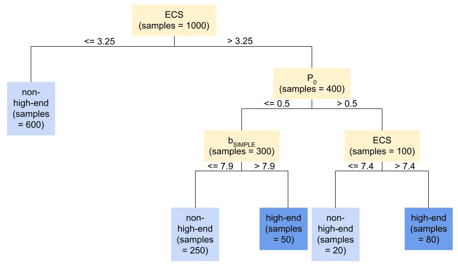
Figure 1 Hypothetical decision tree demonstrating the general decision tree structure using BRICK model parameters and our high-end and non-high-end classification outcomes. Since we used a maximum depth of 3 as the stopping criterion, the tree made three levels of splits before stopping to create leaf nodes.

2.3 Random forests

As can be the case with many machine learning algorithms, decision trees can overfit the training data used to create the tree (James et al., 2013). Random forests, which are an ensemble method, are one way to reduce overfitting. Random forests are a collection of many decision trees, created by using a random subset of the training data to build each tree and by using a random subset of the features at each split. Taking a random subset of the training data when creating a tree is called bootstrapped aggregation, or bagging. When bagging, the random subset of the training data is taken with replacement. In addition to bootstrap subsets of training data, random forests take a random subset of features from which to split the data. This further helps to address the issue of overfitting the training data. In this work, the features of the random forests are the parameters of the BRICK model, and the response to be classified is whether or not the time series of GMSL associated with those parameters is a high-end GMSL scenario (above the 90th percentile).

The following general process outlines how we construct each random forest. We repeat this process to classify the high-end GMSL scenarios in 5-year increments from 2020 through 2150 for each of RCP2.6 and RCP8.5. This leads to a total of 27 random forests for each of the two RCP scenarios.

To create a random forest of decision trees, we first split the data (after replication to balance the data between classes) into the parameters and the output for the given year. We then created training, validation, and test subsets of those data. The training set is used to train the model, the validation set is used to tune the model's hyperparameters, and the test set is used to test the model's performance. In this work, the training subset comprises 60 % of the original data, the validation subset is another 20 %, and the test is also 20 % of the original full data set. This follows the convention that training data should comprise 50 % to 75 % of the data (Hackeling, 2017). We use the RandomForestClassifier from the sklearn.ensemble library to make a forest of decision trees using entropy as the criterion to determine the splits of each tree (Pedregosa et al., 2011).

Prior to fitting the model, we tune the hyperparameters of the RandomForestClassifier by performing a grid search. For each hyperparameter combination in the grid, a random forest is constructed using the training data and evaluated using the validation data. The performance on the validation data determines the best values of the hyperparameters to use when constructing our forest. In addition to the three decision-tree-specific hyperparameters noted in Sect. 2.2, we explored values for the following parameters in our grid search:

• max_features, the number of features a tree can consider at each split, and

• n_estimators, the numbers of trees in the forest (Pedregosa et al., 2011).

We performed grid searches using the ranges shown in Table 1 on RCP2.6 and RCP8.5 in the year 2100. These cases were chosen to simplify the hyperparameter tuning and because sea-level rise (SLR) literature focuses on the projections in the year 2100. While the default value for max_features is “sqrt” (which equals a value of 6 for our features), we elected to search over values up to the maximum features of 38. A higher value of max_features could improve our model performance, but a lower value creates trees that are less correlated, hence decreasing the testing error (Probst et al., 2019; James et al., 2013). Likewise, a lower value is useful when there are many correlated features, which is the case with the BRICK model (James et al., 2013). We hold min_impurity_decrease at a value of 0.001 to reduce the opportunity for the decision trees to have node splits that do not appreciably improve the quality of the tree.

Both grid searches in the year 2100 yielded the same hyperparameter values as the best set of hyperparameter values (see Table 1). The performance on the validation data sets of the other high ranking hyperparameter combinations produced similar results to these best hyperparameter values. Thus, our model is not sensitive to changing the hyperparameters over the year 2100.

Table 1 Hyperparameter values of the best estimator from the grid search.

Using the random forest hyperparameters settings from the “Best value” row of Table 1, we fit random forests using the training data for each of the 5-year intervals for each of RCP2.6 and 8.5. We input the corresponding testing parameter values into the random forest models for them to predict output values. We then compare the predicted values to the actual output values from the testing data and calculate the percentage of the testing values that the model correctly predicted. The same process is done for the training subset that was used to create the forest. The training, validation, and testing accuracies for the forests can be found in Table A2. Likewise, the confusion matrices for the years 2050, 2100, and 2150 for both RCP scenarios can be found in Figs. A2 and A3, which show that both the negative predictive power and positive predictive power are strong. Using the test data, the positive predictive power ranges from 99.37 % to 100 % in RCP2.6 and ranges from 99.83 % to 100 % in RCP8.5. Meanwhile, the negative predictive value ranges from 94.53 % to 97.38 % in RCP2.6 and 93.6 % to 95.61 % in RCP8.5.

Given the initial hypothesis that the ECS parameter is an important indicator of future sea-level rise (Vega-Westhoff et al., 2020), we examine the set of all split values for the ECS parameter for each tree in the forest. Likewise, we examine the distribution of the maximum ECS value of each tree in the forest. The maximum split values are informative because they differentiate the highest cases of sea-level rise when the trees are branching. Hence, the maximum splits help quantify the threshold of ECS that separates the high-risk situations from the non-high-risk (lower) ECS splits.

2.4 Feature importances

We use feature importances to assess which parameters play the largest role in determining whether or not a given SOW is a high-end GMSL scenario. We compute the importances for each feature (i.e., BRICK model parameter) using our forests fit for each year from 2020 to 2150 in 5-year increments. We use Gini importances as the feature importances, which are the normalized reductions of node impurity by each feature chosen for splitting the tree (Pedregosa et al., 2011). While other importance measures, such as Sobol' sensitivity indices (Sobol', 2001), are based on a decomposition of variance in a distribution of model outcomes, the Gini importances depend on the prediction ability of random forests. The random forest model is trained to be able to predict the outcomes associated with potential parameter values. The Gini importances, in turn, are determined based on the trained random forest model and the roles played by each parameter (in this case, the features).

We calculate the Gini importance of each node in a tree using Eq. (1).

$$\begin{array}{}\text{(1)}& {\text{ni}}_j=w_j{C}_j-w_{\text{left},j}{C}_{\text{left},j}-w_{\text{right},j}{C}_{\text{right},j}\end{array}$$

ni_j is the node importance of node j, w_j is the weighted number of samples at node j, C_j is the impurity of node j, the “left” subscript represents the left child from the split on node j, and the “right” subscript represents the right child from the split on node j. The weighted number of samples is used as a coefficient of the different impurity calculations because the impurities of nodes address the proportion of data points that belong to that node's left and right children but do not address the total number of data points associated with that node. The calculation of ni_j in Eq. (1) addresses this by giving greater weight to nodes with a large proportion of the samples than nodes that split small numbers of samples.

For example, in Fig. 1, the root node is the ECS split with a value of 3.25 ^∘C. Considering that node, the node importance is described by the equation below.

$$\begin{array}{ll}{\displaystyle }{\text{ni}}_{\text{ECS},\mathrm{3.25}}=& {\displaystyle }\mathrm{1000}{C}_{\text{ECS},\mathrm{3.25}}-\mathrm{600}{C}_{\text{left};\text{ECS},\mathrm{3.25}}\\ {\displaystyle }& {\displaystyle }-\mathrm{400}{C}_{\text{right};\text{ECS},\mathrm{3.25}}\end{array}$$

The impurity of a node is a measure of the efficacy of the feature used for splitting the data set at that node for subdividing the data set. We use entropy as the impurity criterion in our forests, which ranges in value from 0 to 1. If the data at a given node are split evenly among that node's left and right children, then the node impurity is maximized at 1. The more asymmetrically the data at that node are split between the node's children, the lower the node's entropy will be. The closer the entropy is to 1, the more difficult it is to draw conclusions from the data split by that node. We calculate entropy using Eq. (2), where p_c is the fraction of examples in class c (where c here is either high-end GMSL or non-high-end GMSL).

$$\begin{array}{}\text{(2)}& C_j=\text{entropy}=-\sum _c{p}_c{\log }_{\mathrm{2}}\left(p_c\right)\end{array}$$

In the example using Fig. 1, the entropies would be the following:

$$\begin{array}{c}{\displaystyle }\begin{array}{rl}{C}_{\text{ECS},\mathrm{3.25}}=& -\left(p_{\text{high-end}}{\log }_{\mathrm{2}}\right(p_{\text{high-end}})\\ & \phantom{-(}+p_{\text{non-high-end}}{\log }_{\mathrm{2}}\left(p_{\text{non-high-end}}\right))\\ =& -\left({\displaystyle \frac{\mathrm{130}}{\mathrm{1000}}}{\log }_{\mathrm{2}}\left({\displaystyle \frac{\mathrm{130}}{\mathrm{1000}}}\right)+{\displaystyle \frac{\mathrm{870}}{\mathrm{1000}}}{\log }_{\mathrm{2}}\left({\displaystyle \frac{\mathrm{870}}{\mathrm{1000}}}\right)\right)\\ \approx & \mathrm{0.5574}\end{array}\\ {\displaystyle }\begin{array}{rl}{C}_{\text{left};\text{ECS},\mathrm{3.25}}=& -\left(p_{\text{high-end}}{\log }_{\mathrm{2}}\right(p_{\text{high-end}})\\ & \phantom{-(}+p_{\text{non-high-end}}{\log }_{\mathrm{2}}\left(p_{\text{non-high-end}}\right))\\ =& -\left({\displaystyle \frac{\mathrm{0}}{\mathrm{600}}}{\log }_{\mathrm{2}}\left({\displaystyle \frac{\mathrm{0}}{\mathrm{600}}}\right)+{\displaystyle \frac{\mathrm{600}}{\mathrm{600}}}{\log }_{\mathrm{2}}\left({\displaystyle \frac{\mathrm{600}}{\mathrm{600}}}\right)\right)\\ =& \mathrm{0}\end{array}\\ {\displaystyle }\begin{array}{rl}{C}_{\text{right};\text{ECS},\mathrm{3.25}}=& -\left(p_{\text{high-end}}{\log }_{\mathrm{2}}\right(p_{\text{high-end}})\\ & \phantom{-(}+p_{\text{non-high-end}}{\log }_{\mathrm{2}}\left(p_{\text{non-high-end}}\right))\\ =& -\left({\displaystyle \frac{\mathrm{130}}{\mathrm{400}}}{\log }_{\mathrm{2}}\left({\displaystyle \frac{\mathrm{130}}{\mathrm{400}}}\right)+{\displaystyle \frac{\mathrm{270}}{\mathrm{400}}}{\log }_{\mathrm{2}}\left({\displaystyle \frac{\mathrm{270}}{\mathrm{400}}}\right)\right)\\ \approx & \mathrm{0.9097}.\end{array}\end{array}$$

With these, the node impurity of the ECS split with a value of 3.25 ^∘C can be fully calculated as shown in the equations below.

$$\begin{array}{ll}{\displaystyle }{\text{ni}}_{\text{ECS},\mathrm{3.25}}=& {\displaystyle }\mathrm{1000}{C}_{\text{ECS},\mathrm{3.25}}-\mathrm{600}{C}_{\text{left};\text{ECS},\mathrm{3.25}}\\ {\displaystyle }& {\displaystyle }-\mathrm{400}{C}_{\text{right};\text{ECS},\mathrm{3.25}}\\ {\displaystyle }=& {\displaystyle }\mathrm{1000}\left(\mathrm{0.5574}\right)-\mathrm{600}\left(\mathrm{0}\right)-\mathrm{400}\left(\mathrm{0.9097}\right)\\ {\displaystyle }=& {\displaystyle }\mathrm{193.52}\end{array}$$

Once the node importances of a tree are calculated, we use them to calculate feature importances in Eq. (3).

$$\begin{array}{}\text{(3)}& {\text{fi}}_i={\displaystyle \frac{{\sum }_{j:\text{node}j\text{splits on feature}i}{\text{ni}}_j}{{\sum }_{n\in \text{all nodes}}{\text{ni}}_n}}\end{array}$$

In Eq. (3), fi_i is the feature importance of feature i. The feature importances are normalized so they sum to 1. Equation (4) demonstrates normalizing the previously calculated feature importances.

$$\begin{array}{}\text{(4)}& {\text{fi}}_{i,\text{normalized}}={\displaystyle \frac{{\text{fi}}_i}{{\sum }_{k\in \text{all features}}{\text{fi}}_k}}\end{array}$$

Since we are constructing forests of trees, the feature importances that we present for a given forest are the mean feature importances over all the trees in the forest.

We compute the feature importances for each feature for each forest that we fit, in 5-year intervals from 2020 to 2150. With these importances, we construct a stacked bar graph from 2020 to 2150 in 5-year increments. The bar for each year shows the breakdown of the feature importances for that specific year. Hence, all of the individual feature importances bars for a given year will add up to 1. We define an “other” category such that model parameters with an importance less than 4 % are grouped into “other”. There are 38 model parameters, so if the importances were uniform across all the parameters, each importance would be about 2.6 %. Hence, any “other” category threshold of 3 % or less would show importances that were not substantially different from the average. Because of that, we use 4 % as the threshold for the “other” category.

It is important to note that when parameters are grouped into the “other” category, it does not necessarily mean that the values of those parameters can be fixed at any value. It may mean, however, that the GMSL output that we are using in this work, which is just one of the multiple outputs of the BRICK model, is not sensitive to that specific parameter. A parameter could also be grouped into the “other” category because it is well constrained with relatively low uncertainty in addition to the GMSL output uncertainty not greatly depending on the uncertainty of that input parameter.

3 Results

3.1 Feature importances

Based on Fig. 2, ECS (darkest stippled blue boxes) and the aerosol scaling factor (α_DOECLIM) (solid blue boxes) are consistently associated with the greatest high-end sea-level hazard throughout both RCP2.6 and RCP8.5. Both of these model parameters are associated with the climate component of the BRICK model. In RCP2.6, ECS accounts for 15.1 % of the overall feature importance in the year 2020 and increases to 44.4 % by the year 2150 (Fig. 2a). Likewise, the aerosol scaling factor (α_DOECLIM) accounts for 5.0 % of the overall feature importance in 2025 and increases to 11.5 % by the year 2150 (Fig. 2a). In the higher-forcing RCP8.5 scenario, ECS accounts for 14.0 % and α_DOECLIM accounts for 4.6 % of the overall feature importance in 2020. By 2150 in RCP8.5, they increase to 21.7 % and 12.1 % respectively (Fig. 2b). The importance of the aerosol scaling factor (α_DOECLIM) is perhaps unsurprising, given that the uncertainty range in this parameter in previous work (e.g., Urban and Keller, 2010; Wong et al., 2017b) encompasses both positive and negative effects on net total radiative forcing. This parameter accounts for feedbacks from aerosol–cloud interactions and indirect effects from aerosols on radiative forcing (Hegerl et al., 2006; Lohmann and Feichter, 2005). These effects can vary widely and can depend on the specific representation of the cloud feedback processes incorporated into more detailed global climate models (Wang et al., 2021). The relatively higher importance associated with these climate module parameters in the lower-forcing RCP2.6 scenario is indicative of the large influence exerted by those parameters on the severity of the resulting sea-level rise. The only parameter in RCP2.6 that has an importance noticeably greater than 4 % and belongs to a non-climate component of BRICK is the temperature associated with AIS fast disintegration, T_crit (Fig. 2a). This suggests that in the high-end SOW of sea-level rise, even in the low-forcing RCP2.6 scenario, by the middle of the 21st century and beyond, the AIS dynamics can still drive severe risks to coastal areas.

In a supplemental experiment, we used 80th percentile of GMSL to classify the high-end and non-high-end cases. We find that the patterns emerging from the feature importances using the random forests fitted using the 80th percentile of the data are comparable to that of the 90th percentile (Fig. A1). Hence, our results are not sensitive to our choice to use the 90th percentile.

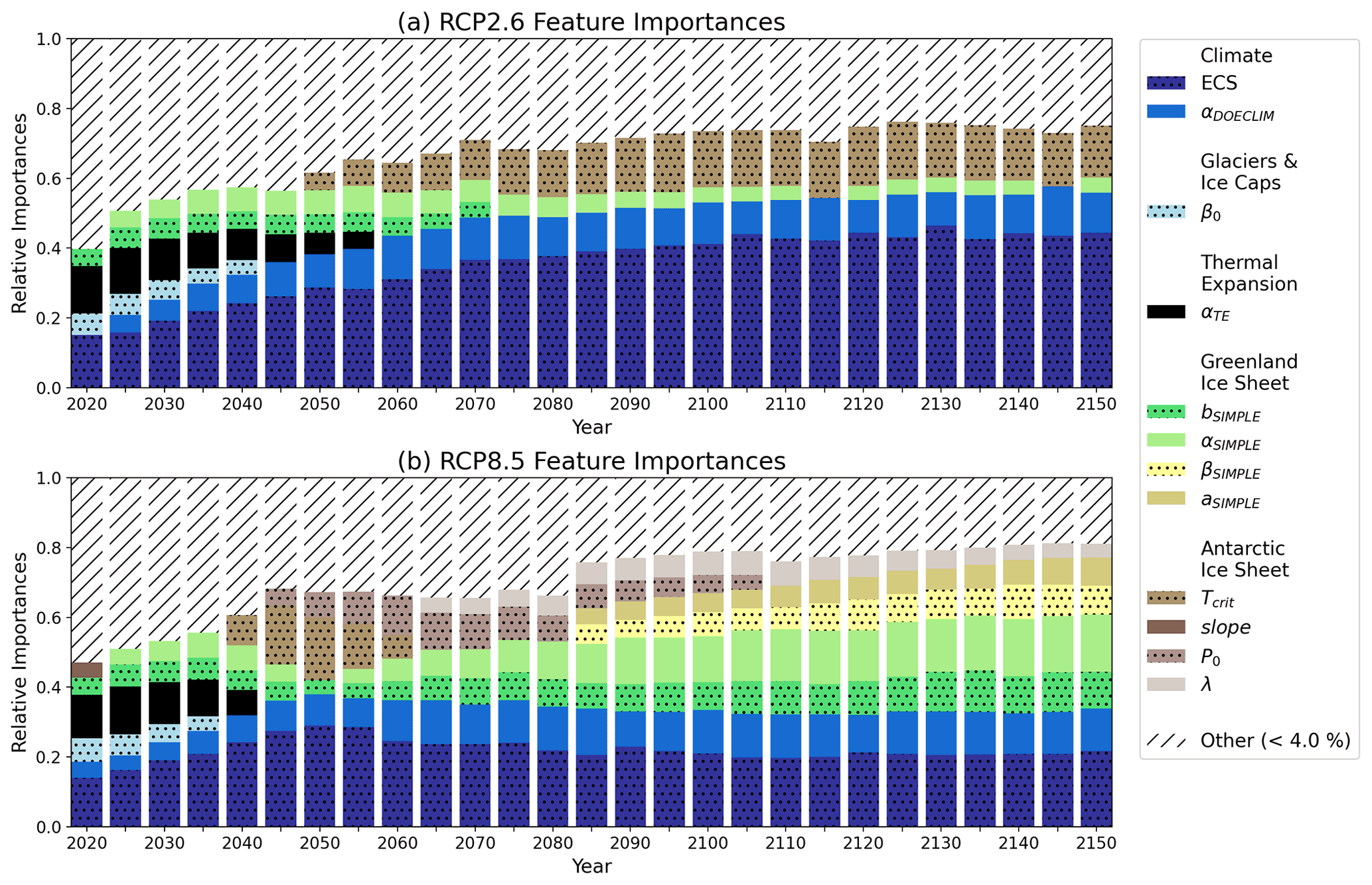
Figure 2 Relative feature importances of the BRICK model parameters calculated based on the fitted random forests. Shown are the importances of the BRICK model parameters using (a) the RCP2.6 radiative forcing scenario and (b) the RCP8.5 forcing scenario. All model parameters with an importance less than 4 % were grouped into an “other” category, which is shown with hatch marks to denote its difference from the parameters. Stippling was added to alternating parameters in the legend to aid in telling the difference between similar colors. An “other” threshold of 4 % was chosen because uniform importance across the parameters is 2.6 % importance for each parameter. Using a threshold close to 2.6 % would show parameters that were not substantially different than the average importance.

3.2 Characterization of risk over time

In contrast to high-end sea-level rise being driven primarily by climate uncertainties under RCP2.6, in the higher-forcing RCP8.5 scenario, the importances of the ECS and aerosol scaling factor are relatively lower. This is indicative of the transition to uncertainty in sea-level processes driving high-end risks under the higher-forcing scenario.

The near-term risk in both RCP2.6 and RCP8.5 is driven by sea-level rise from thermal expansion (α_TE) (solid black boxes) and mass loss from glaciers and ice caps (β₀) (stippled light blue boxes). Figure 2 shows that the parameters related to thermal expansion are important from 2020 until the middle of the century, becoming less important as time goes on. In RCP2.6, α_TE comprises 13.5 % of the overall feature importance in 2020, which then decreases to 4.9 % in 2055. Likewise in RCP8.5, α_TE accounts for 12.3 % in 2020 and decreases to 7.2 % in 2040. Thermal expansion will even occur in low-emission scenarios such as RCP2.6 due to inertia. Mengel et al. (2018) find that “thermal expansion, mountain glaciers, and the Greenland ice sheet continue to add to sea-level rise under temperature stabilization”. The importance of thermal expansion decreases over time because there are much more sizable contributions to sea-level rise from the ice sheets. This increase in contribution from the ice sheets is due to them being triggered. The ice sheets are triggered once we surpass the tipping point for them (Lenton et al., 2019).

Similar to thermal expansion, mass loss from glaciers and ice caps is important starting in 2020 and decreases in importance over time. In RCP2.6, β₀ accounts for 6.2 % of the overall feature importance in 2020 and decreases to 4.2 % in 2040. Meanwhile in RCP8.5, β₀ comprises of 6.8 % in 2020, which decreases to 4.3 % in 2035.

As for the long-term risks, ice loss from AIS is a driver in both emissions scenarios. In particular, the T_crit and λ parameters within the AIS component of BRICK are important (Fig. 2, solid dark brown boxes and solid taupe respectively). Within the BRICK model, T_crit is the temperature associated with the onset of fast dynamical disintegration of AIS. In RCP8.5, T_crit is significantly important from 2040 to 2060. This is consistent with predictions that major AIS disintegration will occur between 2040 and 2070 in high radiative forcing scenarios (Kopp et al., 2017; DeConto et al., 2021; Wong et al., 2017a; Nauels et al., 2017b).

In addition to AIS, ice loss from GIS also poses a risk in the long term. In the case of GIS, the sea-level rise associated with its ice loss only has significant importance in RCP8.5. The specific model parameters associated with the Greenland ice sheet are the following: b_SIMPLE, α_SIMPLE, β_SIMPLE, and a_SIMPLE (Fig. 2b; stippled green boxes, solid light green boxes, stippled yellow boxes, and solid tan boxes respectively).

This follows with the work of Wahl et al. (2017) that found uncertainty stemming from GIS is greater in higher-forcing RCP scenarios. In Fig. 2, the importance of GIS is much more prominent in RCP8.5 than RCP2.6. While the importance decreases over time in RCP2.6, it increases over time in RCP8.5. By 2100 in RCP8.5, it comprises 33.5 % of the overall feature importances, and by 2150, it grows to 43.3 % of the overall importance. This is likely attributable to the fact that the Greenland ice sheet mass balance may cross tipping points related to surface ice melt as early as 2030 under higher forcing (Lenton et al., 2019). Additionally, uncertainty in the magnitude of, the timing of, and the degree to which we surpass these tipping points compound, leading to greater uncertainty in ice sheet contributions to sea-level rise this century (Robinson et al., 2012). The sizable uncertainties attributable to the Greenland and Antarctic ice sheet contributions to global sea-level change are in line with previous assessments that compared the uncertainties in different components of sea-level rise (Wahl et al., 2017; Mengel et al., 2016). Specifically, higher uncertainties in higher-forcing scenarios are broadly consistent with the projections by other semi-empirical models for sea-level rise (e.g., Mengel et al., 2016).

Overall, it is expected that the uncertainty in GIS impacts future GMSL. P. Bakker et al. (2016) noted that uncertainty in GIS is a key driver of uncertainty in future Atlantic Meridional Overturning Circulation (AMOC) strength. AMOC strength, in turn, is critically linked to transport of heat meridionally across the Atlantic Ocean. Similarly, Wong and Keller (2017) performed a case study for New Orleans, Louisiana, which found that GIS may be of second-order importance for local flood hazard behind uncertainties from AIS and the storm surge. In this study, GIS only showed importance in the variance-based sensitivity analysis when the storm surge parameters were removed from the analysis.

For both GIS and AIS, the uncertainty in future GMSL contributions from these ice sheets dynamics compounds with uncertainty in future temperatures on which these dynamics rely (Jevrejeva et al., 2018; Robinson et al., 2012).

3.3 ECS threshold of high-end sea-level rise

Previous work by Vega-Westhoff et al. (2020) used 5 ^∘C as the value of ECS that separates high-end and non-high-end climate risk scenarios. Using our collection of random forests, we select the highest ECS split value that each decision tree in the forest split on. These split values should separate the highest-risk scenarios of GMSL in each time interval. Figure 3 shows the distribution of the maximum ECS splits for every 5 years in the 2020 to 2150 time period.

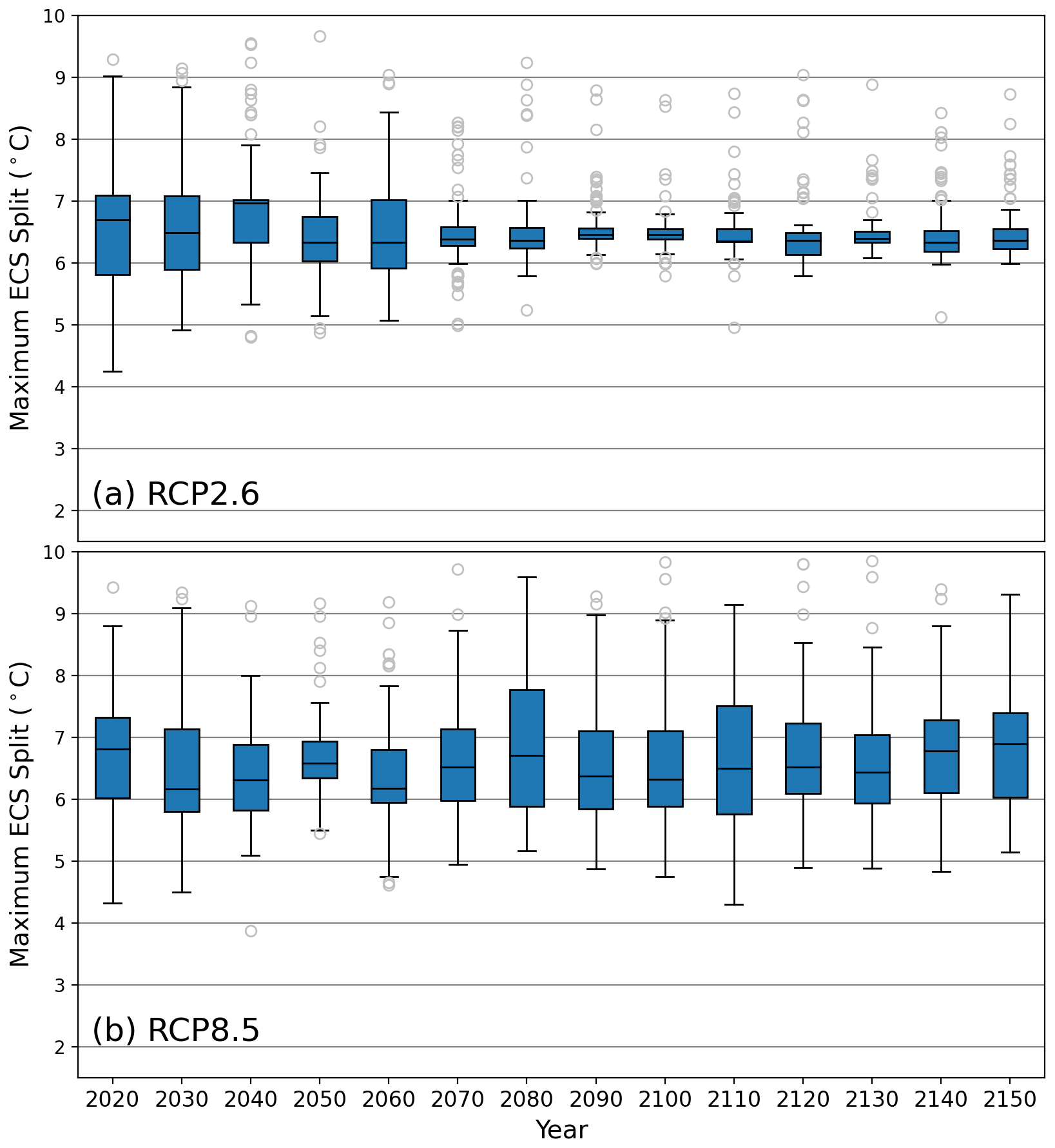
Figure 3 Distributions of the maximum equilibrium climate sensitivity (ECS) split value from each decision tree in the fitted random forests. Panel (a) depicts the maximum ECS split distributions in the RCP2.6 forests, and panel (b) depicts the maximum ECS split distributions in the RCP8.5 forests. The outliers are the data points less than $\text{Q1}-\mathrm{1.5}\cdot \text{IQR}$ or greater than $\text{Q3}+\mathrm{1.5}\cdot \text{IQR}$, where Q1 is quartile 1, Q3 is quartile 3, and IQR is the interquartile range (Q3−Q1). The blue boxes show the IQR, and the line within the IQR is the median.

There is a considerable number of outliers of the maximum ECS split value in RCP2.6, particularly in the high-risk upper tail (Fig. 3a). However, the interquartile ranges are quite small. In most cases, the interquartile range for RCP2.6 falls between approximately 6 and 7 ^∘C (Fig. 3a). The greatest interquartile range width is 1.3 ^∘C in 2020, and the smallest width is 0.2 ^∘C in 2100, with an average of 0.5 ^∘C (Table A3). Likewise, the median is consistently between 6.25 and 6.5 ^∘C. In RCP2.6, the median of the maximum ECS split over the given years ranges from 6.3 to 7.0 ^∘C (Table A3).

There are fewer outliers in RCP8.5 than in RCP2.6, but RCP8.5 has wider uncertain ranges. The interquartile ranges of the maximum ECS split value in RCP8.5 span a larger length than those of RCP2.6. Here, the interquartile ranges are mostly contained between 5.75 and 7.5 ^∘C (Fig. 3b). The interquartile range width in RCP8.5 is between 0.6 ^∘C (in 2050) and 1.9 ^∘C (in 2080), with an average of 1.2 ^∘C (Table A3). However, the median is consistently between 6.25 and 7 ^∘C. In RCP8.5, the median of the maximum ECS split over the given years ranges from 6.2 to 6.9 ^∘C (Table A3).

Since the median is consistently between 6.25 and 6.5 ^∘C in the low radiative forcing scenario and between 6.25 and 7 ^∘C in the high radiative forcing scenario, our random forests suggest that an ECS value of approximately 6.5 ^∘C could be used as a threshold for high-end scenarios of global mean sea-level rise to reconcile the differences between RCPs. In a supplemental experiment, we reproduced the same experiment using the 80th percentile of the global mean sea level to denote the high-end cases (as opposed to the 90th percentile in the main experiments). We find that the distribution of the maximum ECS split value from each decision tree in the random forests fitted using the 80th percentile of the data is very similar to that of the 90th percentile (Fig. A5). Hence, our results are not sensitive to our choice to use the 90th percentile.

4 Conclusions

In this work, we present an approach to classify global mean sea level from the BRICK semi-empirical model as either high-end or non-high-end. We use a previously published model output data set to construct random forests for 5-year increments from 2020 to 2150 for RCP2.6 and RCP8.5. We explore the parametric drivers of risk by examining the feature importances of random forests. Results show that climate components of the BRICK model, specifically equilibrium climate sensitivity (ECS) and the aerosol scaling factor (α_DOECLIM), are consistently the most important parametric uncertainties in both radiative forcing scenarios (Fig. 2). Our results also show that thermal expansion and glacier and ice cap mass loss both pose a risk in the near-term and that long-term risks are driven by mass loss from the Greenland and Antarctic ice sheets (Fig. 2). Nicodemus et al. (2010) found that random forests are more likely to select correlated features as the first split in the tree. We performed an experiment using permutation importance, a suggested alternative by Strobl et al. (2007), as the measure of feature importance and found similar results to the Gini importances (Fig. A6).

In addition to the feature importances, we find that an ECS value greater than 6.25 to 6.5 ^∘C indicates a high-end sea-level rise scenario based on the maximum ECS split values that each decision tree in a forest splits on (Fig. 3). This result is consistent for both RCP2.6 and RCP8.5, as well as when using the 80th or 90th percentile to characterize the sea-level data as high-end.

These results demonstrate the nonstationary risks posed by climate change and the related hazards driven by sea-level change. In turn, climate risk management strategies must address near-term actions to mitigate near-term risks such as sea-level rise from thermal expansion and glaciers and ice caps. At the same time, risk management strategies must also guard against the long-term risks driven by mass loss from the major ice sheets. While this work was centered around the impact of model parametric uncertainties on sea-level hazards, the same machine learning approaches can be generalized to incorporate the socioeconomic uncertainties that relate future climate hazards (e.g., changes in temperatures and sea levels) to financial and human risks. These approaches offer promise to provide a more holistic view of uncertainties affecting future climate risk and the efficacy of human strategies to mitigate and manage these risks.

Appendix A

Table A1 Hector–BRICK model parameter names, units, and descriptions (Vega-Westhoff et al., 2019).

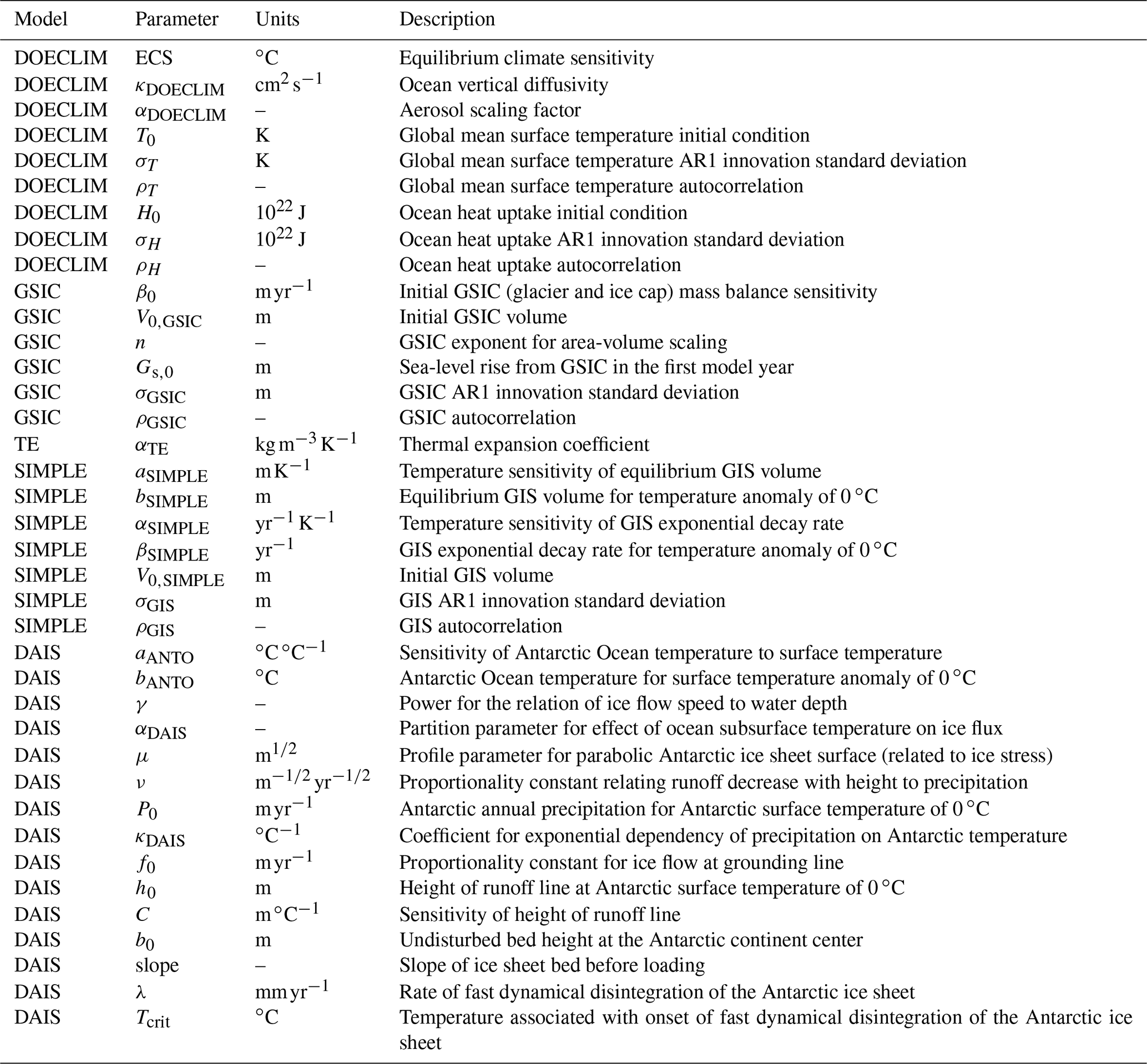
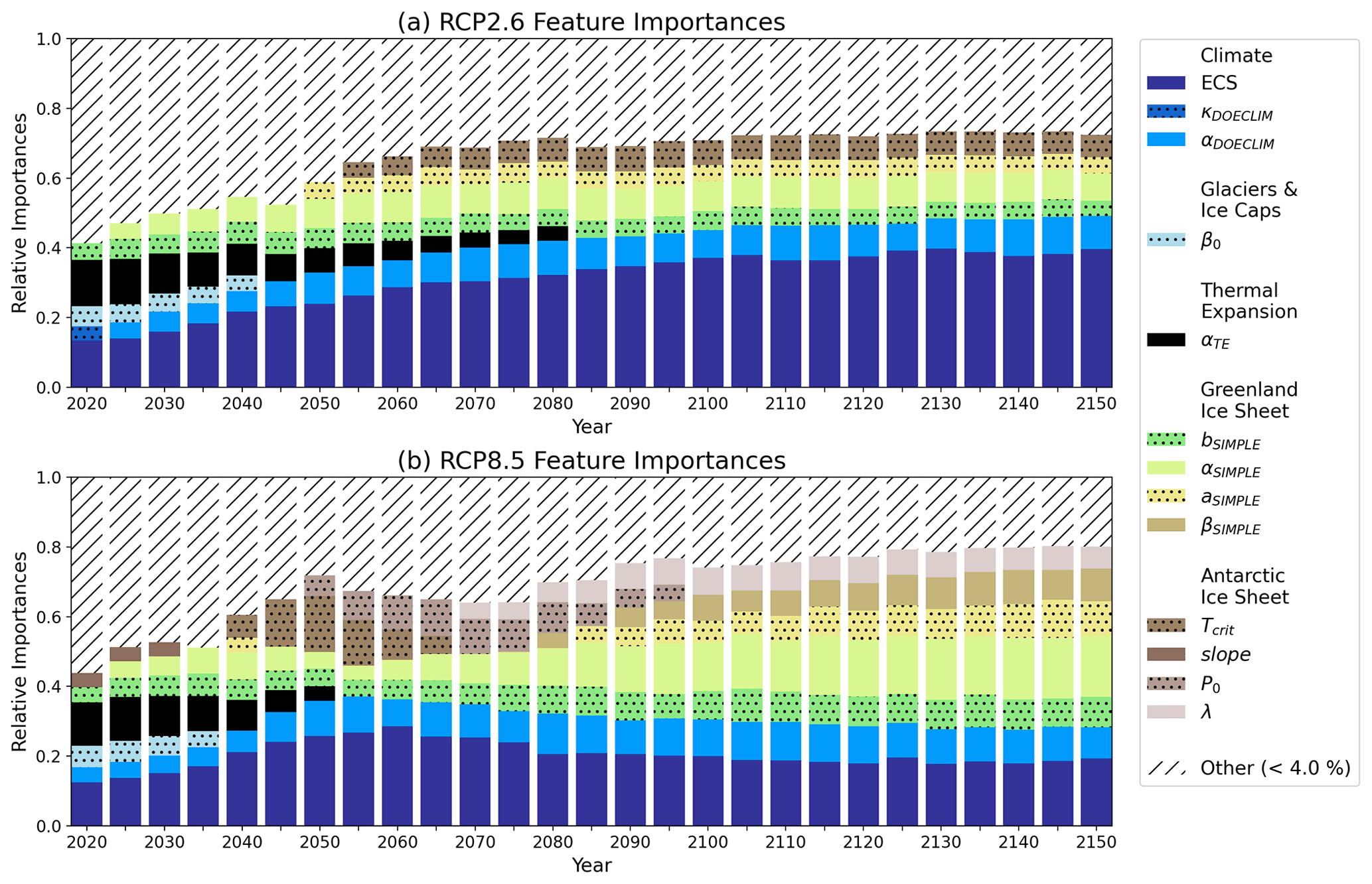
Figure A1 Relative feature importances of the BRICK model parameters calculated based on the random forests fitted when defining the high-end threshold as the 80th percentile of the data. Shown are the importances of the BRICK model parameters using (a) the RCP2.6 radiative forcing scenario and (b) the RCP8.5 forcing scenario. All model parameters with an importance less than 4 % were grouped into an “other” category, which is shown with hatch marks to denote its difference from the parameters. Stippling was added to alternating parameters in the legend to aid in telling the difference between similar colors.

Table A2 Random forests' accuracy on the training, validation, and testing subsets.

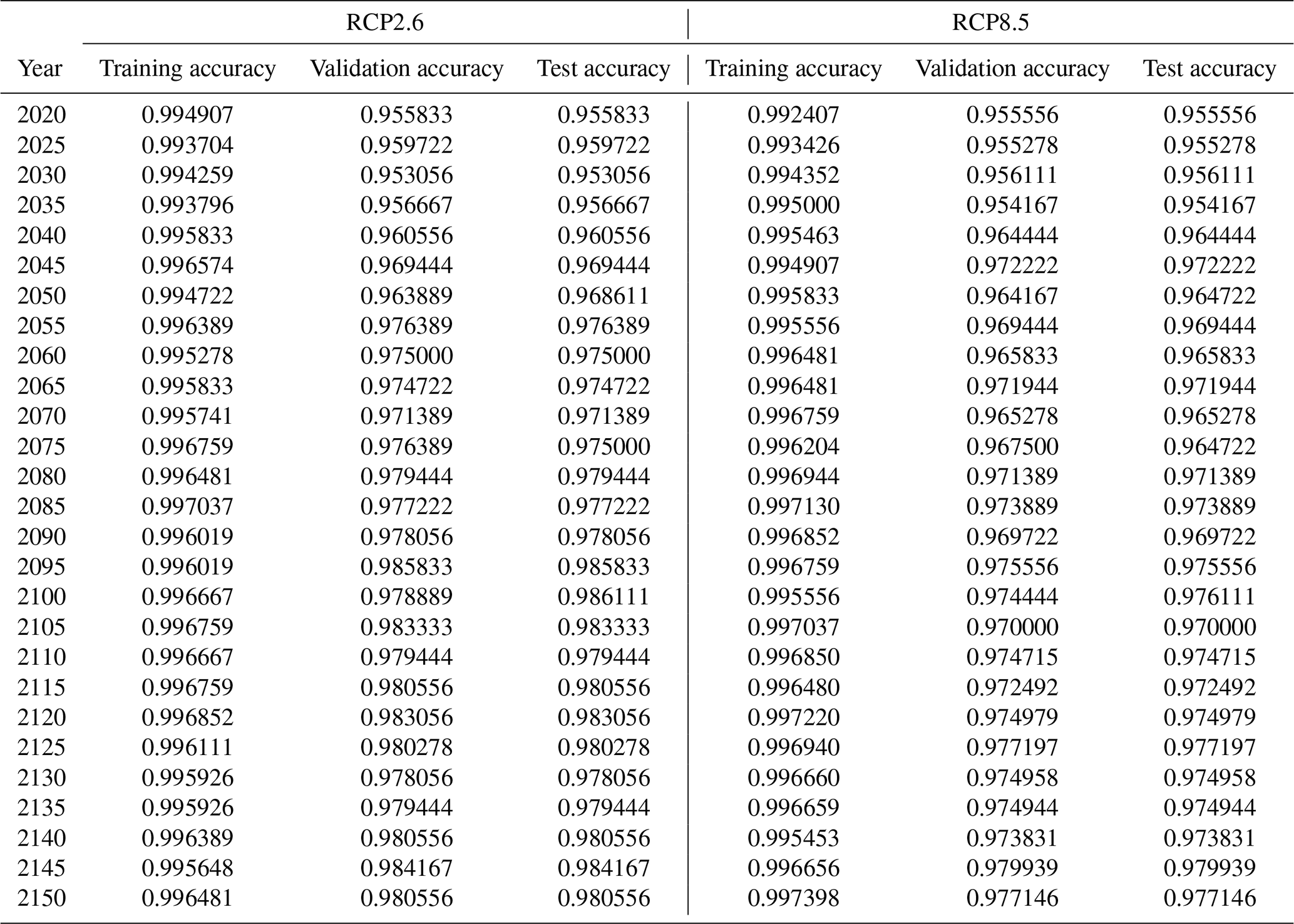
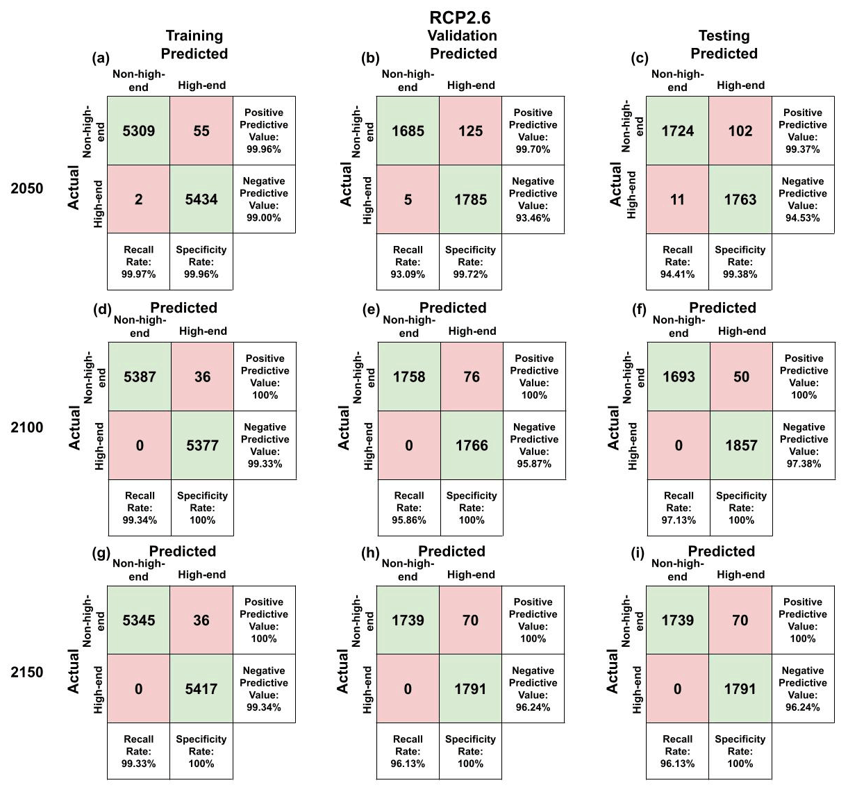
Figure A2 Random forests' confusion matrices on the RCP2.6 training, validation, and testing subsets.

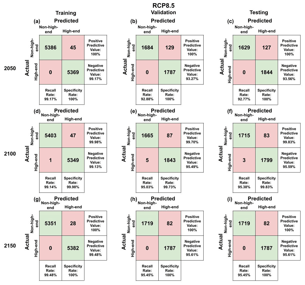
Figure A3 Random forests' confusion matrices on the RCP8.5 training, validation, and testing subsets.

Table A3 Quartile descriptions of the distributions of the maximum equilibrium climate sensitivity (ECS) split value from each decision tree in the fitted forests. Q1 denotes quartile 1, which is the 25th percentile of the data. The median is the 50th percentile of the data. Q3 denotes quartile 3, which is the 75th percentile of the data. IQR stands for the interquartile range, which is calculated as Q3−Q1.

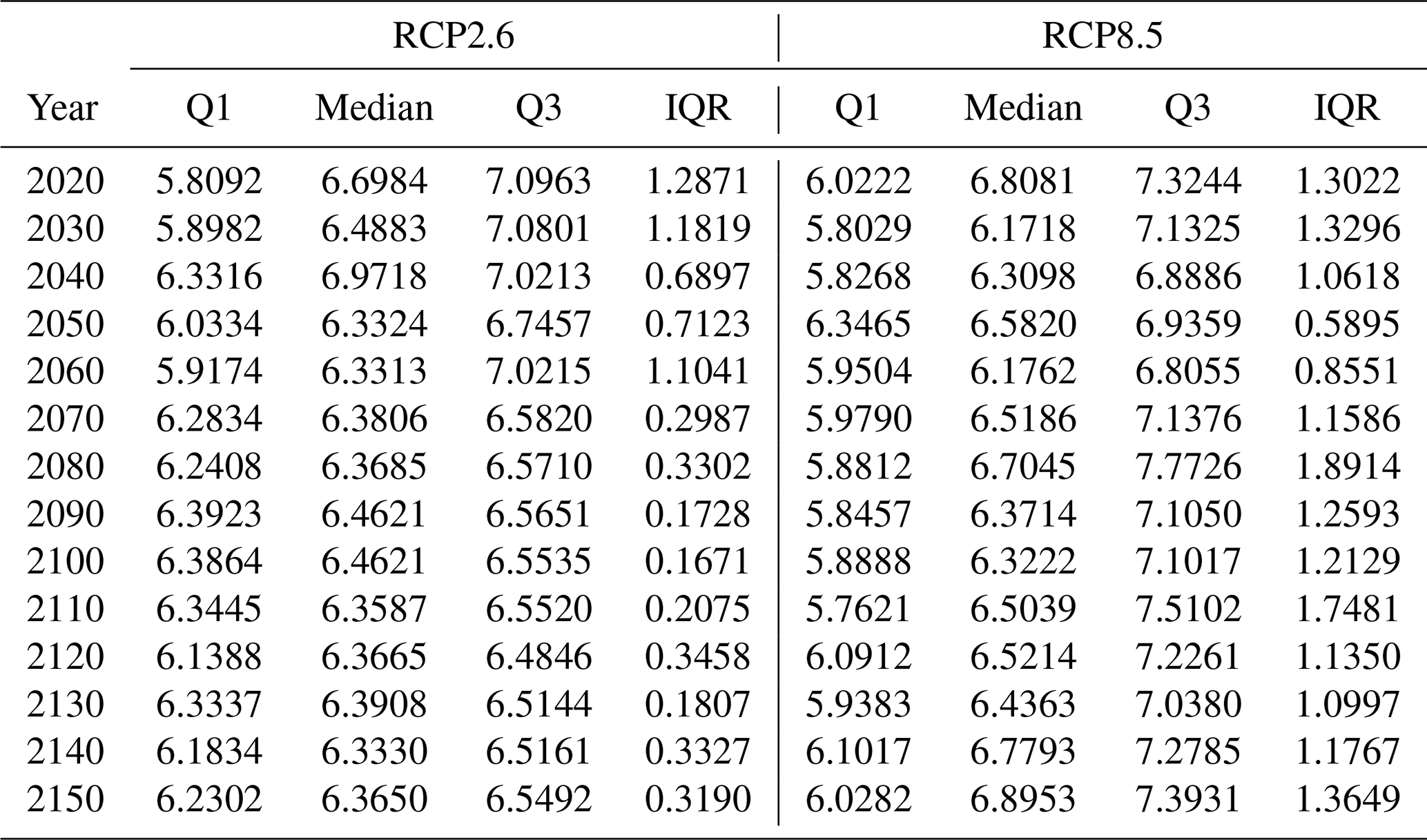
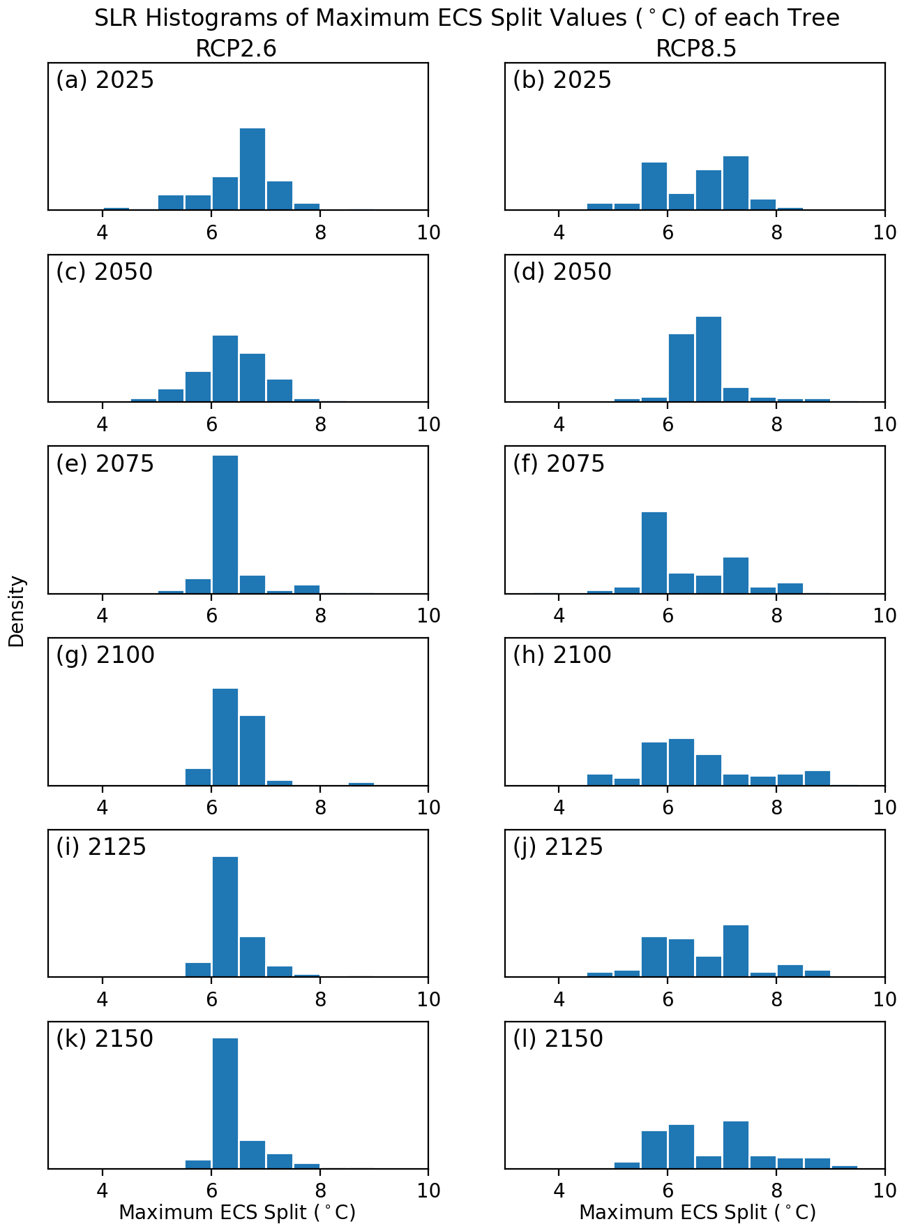
Figure A4 Distributions of the maximum equilibrium climate sensitivity (ECS) split value from each decision tree in the fitted random forests. The left column of plots depicts the maximum ECS split distributions in the RCP2.6 forests, and the right column depicts the maximum ECS split distributions in the RCP8.5 forests.

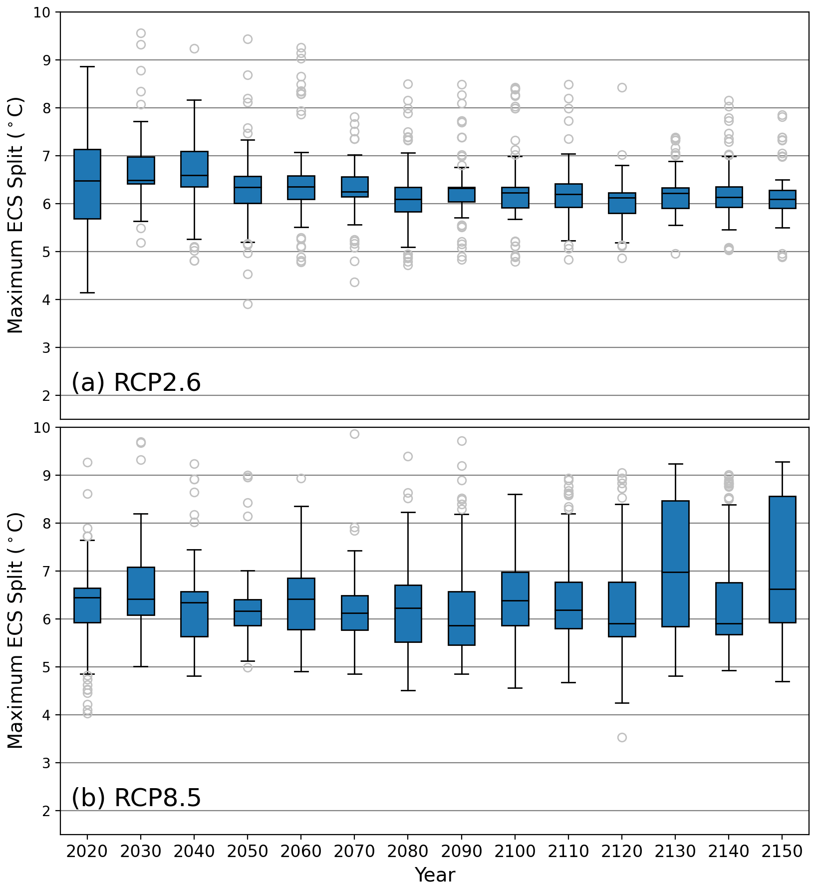
Figure A5 Distributions of the maximum equilibrium climate sensitivity (ECS) split value from each decision tree in the random forests fitted using the 80th percentile to classify the GMSL data. Panel (a) depicts the maximum ECS split distributions in the RCP2.6 forests, and panel (b) depicts the maximum ECS split distributions in the RCP8.5 forests. The outliers are the data points less than $\text{Q1}-\mathrm{1.5}\cdot \text{IQR}$ or greater than $\text{Q3}+\mathrm{1.5}\cdot \text{IQR}$, where Q1 is quartile 1, Q3 is quartile 3, and IQR is the interquartile range (Q3–Q1). The blue boxes show the IQR, and the line within the IQR is the median.

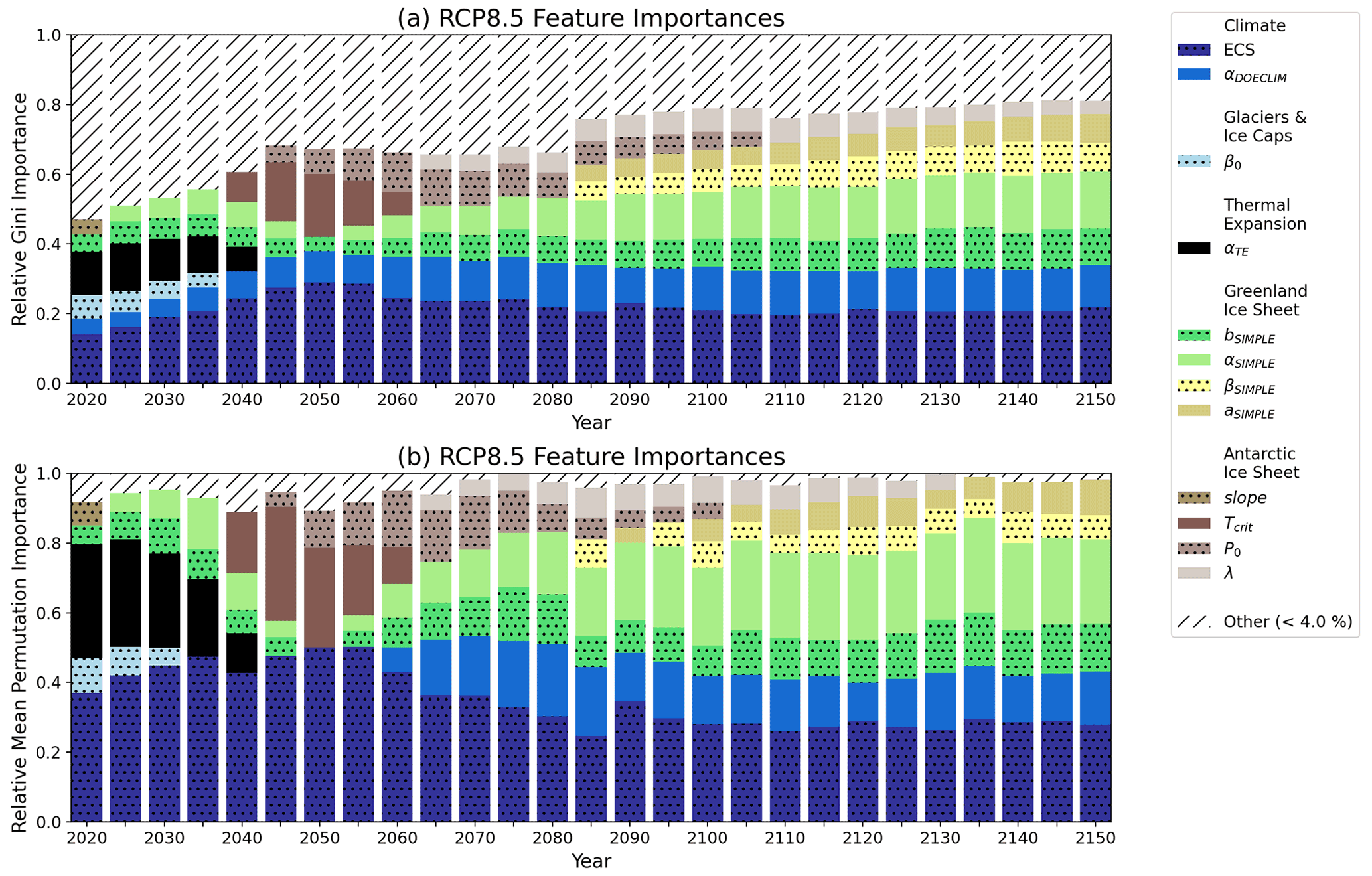
Figure A6 Relative feature importances of the BRICK model parameters calculated based on the fitted random forests using different feature importance measures. Shown are the importances of the BRICK model parameters using (a) the RCP8.5 radiative forcing scenario with Gini importances and (b) the RCP8.5 forcing scenario with permutation importances. All model parameters with an importance less than 4 % were grouped into an “other” category, which is shown with hatch marks to denote its difference from the parameters. Stippling was added to alternating parameters in the legend to aid in telling the difference between similar colors.