the Creative Commons Attribution 4.0 License.
the Creative Commons Attribution 4.0 License.
 | 01 Sep 2022
Statistical reconstruction of European winter snowfall in reanalysis and climate models based on air temperature and total precipitation
Flavio Maria Emanuele Pons
Davide Faranda
The description and analysis of compound extremes affecting mid- and high latitudes in the winter requires an accurate estimation of snowfall. This variable is often missing from in situ observations and biased in climate model outputs, both in the magnitude and number of events. While climate models can be adjusted using bias correction (BC), snowfall presents additional challenges compared to other variables, preventing one from applying traditional univariate BC methods. We extend the existing literature on the estimation of the snowfall fraction from near-surface temperature, which usually involves binary thresholds or nonlinear least square fitting of sigmoidal functions. We show that, considering methods such as segmented and spline regressions and nonlinear least squares fitting, it is possible to obtain accurate out-of-sample estimates of snowfall over Europe in ERA5 reanalysis and to perform effective BC on the IPSL_WRF high-resolution EURO-CORDEX climate model when only relying on bias-adjusted temperature and precipitation. In particular, we find that cubic spline regression offers the best tradeoff as a feasible and accurate way to reconstruct or adjust snowfall observations, without requiring multivariate or conditional bias correction and stochastic generation of unobserved events.
- Article
(15423 KB) - Full-text XML
- BibTeX
- EndNote


Despite the expectations of less frequent snow events in a warming climate, there are still several motivations to study trends in future snowfall. First of all, snowfall extremes can still have a great impact on economy and society. Recent snowfall over large, populated areas of France in February 2018 and in Italy in January 2017 caused transport disruption, several casualties, and economic damage. Snow is also an important hydrological quantity and crucial for the tourism industry of some countries. Although climate models predict a general reduction in snowfall amounts due to global warming, accurate estimates of this decline heavily depend on the considered model. Moreover, while this prediction is valid at the global scale, there may be regional exceptions, with northern areas receiving more snowfall during the winter. Large discrepancies in snowfall amounts indeed exist for observational or reanalysis datasets: in detecting recent trends in extreme snowfall events, Faranda (2020) has also investigated the agreement between the ERA5 reanalysis and the E-OBSv20.0e gridded observations in representing snowfall. Since direct snowfall measurements were not available for E-OBSv20.0e, all precipitation that occurred on days where the average temperature was below 2 ∘C was considered as snowfall. Faranda (2020) found that observed trends and the agreement in absolute value between the two datasets largely depended on the considered region. Overall, the climatologies of snowfall provided by the two datasets had similar ranges, although ERA5 tended to overestimate snowfall compared to E-OBSv20.0e. Even though such a binary separation of snowfall, using a temperature threshold, seemed a good option to retrieve snowfall data from E-OBSv20.0e, it has obvious limitations. For example, in an event characterized by abundant precipitation but a temperature associated to a roughly 50 % snow fraction, snowfall would be either strongly under- or overestimated. In this paper, we explore the possibility of reconstructing snowfall from bias-corrected temperature and precipitation via adequate statistical methods to obtain an improved estimate compared to raw snowfall simulation from climate models.
Climate models are the primary tool to simulate multi-decadal climate dynamics and to generate and understand global climate change projections under different future emission scenarios. Both regional and global climate models have coarse resolution and contain several physical and mathematical simplifications that make the simulation of the climate system computationally feasible but also introduce a certain level of approximation. This results in biases that can be easily observed when comparing the simulated climate to observations or reanalysis datasets. Therefore, they provide limited actionable information at the regional and local spatial scales. To circumvent this problem, it is of crucial importance to correct these biases for impact and adaptation studies and for the assessment of meteorological extreme events in a climate perspective (see, e.g., Ayar et al., 2016; Grouillet et al., 2016).
In order to mitigate the aforementioned biases, a bias correction (BC) step is usually performed. This step usually consists of a methodology designed to adjust specific statistical properties of the simulated climate variables towards a validated reference dataset in the historical period. The chosen statistics can be very simple, e.g., mean and variance, or it may include dynamical features in time, such as a certain number of lags of the autocorrelation function for time series data, it can be constructed using a limited number of moments or aim at correcting the entire probability distribution of the variable, and the correction can also be carried out in the frequency domain so that the entire time dependence structure is preserved. For an overview of various BC methodologies applied to climate models see, for example, Teutschbein and Seibert (2012, 2013) and Maraun (2016). Key efforts have also been made to bias correct precipitation (Vrac et al., 2016) and for multivariate (i.e., multi-sites and variables) approaches, both in downscaling and BC contexts (Vrac and Friederichs, 2015; Vrac, 2018).
Despite the effort devoted to correcting precipitation bias, only a few studies propose specific BC methods for snowfall data from climate projections. For instance, Frei et al. (2018) propose a bias adjustment of snowfall in EURO-CORDEX models specific to the Alpine region, involving altitude-adjusted total precipitation and a single threshold temperature to separate rain and snow. Krasting et al. (2013) study snowfall in CMIP5 models at the northern hemispheric level, highlighting biases but without suggesting any methodology to reduce them, while Lange (2019) proposes a quantile mapping approach that can be used for univariate BC of snowfall.
Indeed, snowfall presents additional challenges compared to other variables, precluding the use of traditional univariate BC methods. Besides the intermittent and non-smooth nature of snowfall fields – a feature in common with total precipitation – snowfall is the result of complex processes which involve not only the formation of precipitation but also the existence and persistence of thermal and hygrometric conditions that allow the precipitation to reach the ground in the solid state. As a result, snow is often observed in a mixed phase with rain, especially when considering daily data. This phase transition poses additional challenges to the bias correction of snowfall, namely the need of separating the snow fraction, using the available meteorological information. Ideally, methods to perform such a separation, also known as precipitation-phase partitioning methods, should be based on wet-bulb temperature, to which the snow fraction is particularly sensitive (Ding et al., 2014). However, due to the difficulty in estimating this parameter in the case of climate models, the task is usually performed by relying on temperature data. These issues would require the application of multivariate BC methodologies, which are significantly more complex than their univariate counterparts and whose applicability is not yet fully understood (François et al., 2020).
In the following, T denotes the mean daily near-surface temperature, Ptot the total daily precipitation, SF the total daily snowfall, fs denotes the snow fraction, and fr the rain fraction of total precipitation.
The fact that T is an effective predictor of fs was first observed by Murray (1952). This study tried to also link the precipitation phase to other variables, such as the freezing level and the thickness of pressure difference layers (1000–700 and 1000–500 hPa), finding that the near-surface temperature alone is as effective at predicting the snow fraction as the others. Following this result, several authors suggest the use of a binary separation of the snow fraction based on a threshold temperature both in climatological (US Army Corps of Engineers, 1956; de Vries et al., 2014; Zubler et al., 2014; Schmucki et al., 2015) and hydrological (Bergström and Singh, 1995; Kite, 1995) studies. In this setting, a threshold temperature T* is chosen, so that the fraction fs of total precipitation falling as snow is 1 for below and 0 for .
In a hydrological modeling context, Pipes and Quick (1977) proposed a linear interpolation between two threshold temperatures . This method provides a simple, yet more realistic, representation of the relationship between the snow fraction and near-surface temperature, which often resembles an inverse S-shaped curve. L'hôte et al. (2005) find similar S-shaped relationships over the Alps and the Andes, pointing to a broad validity of such an assumption; several other instances of research finding evidence of such a relationship are also mentioned in the following paragraph. An important limitation of this method is that the thresholds Tlow and Thigh are fixed. As reported by Kienzle (2008), Pipes and Quick (1977) use threshold values C and C to estimate snowfall in the U.S. Wen et al. (2013) point out that a similar method had already been implemented by US Army Corps of Engineers (1956), using three different threshold values; this adds parameters to the statistical model, which then requires even more fine-tuning before being applied to prediction. In more recent years, the double threshold method has also been applied to climatological analysis, for example in McCabe and Wolock (2008, 2009), where the authors stress that the choice of the thresholds require an important calibration procedure step. Still in the class of threshold models, Kienzle (2008) uses a parameterization considering a temperature TT at which the precipitation is half rain and half snow and a temperature range TR within which both phases co-exist. This method requires validation, using reliable and sub-daily station data, making it less suited for the characterization of gridded snowfall over large domains in reanalysis or climate models.
Slightly more complex methods aim at reproducing the quasi-smooth shape of the precipitation-phase transition by fitting S-shaped functions to the relationship between T and fs (or fr). For example, Dai (2008) proposes a hyperbolic tangent , while McAfee et al. (2014) choose a logistic function , both fitted via nonlinear least squares (NLSs). Harder and Pomeroy (2013) propose a similar procedure, adopted also by Pan et al. (2016), based on a sigmoidal function , where b and c are parameters calibrated using data from a single location, and Ti is the so-called hydrometeor temperature, i.e., the temperature at the surface of a falling hydrometeor, which is defined by Harder and Pomeroy (2013) as a function of air temperature and humidity. While Harder and Pomeroy (2013) find that this method provides more accurate results compared to simple and double thresholds, the estimation of Ti requires reliable measurements or predictions of relative humidity, making this technique more suited to treating observational data.
Wen et al. (2013) present a comparison of some of these methods. In particular, this study examined the model-generated snowfall using different models (namely a regional model with no atmosphere–surface coupling forced by observations and a coupled regional circulation model with land interaction) and assumed forms of fs. The methods put to the test are single threshold (with T* taken to be 0 and 2.5 ∘C), double threshold, both with the parameter values fixed by US Army Corps of Engineers (1956) and Pipes and Quick (1977), and the method proposed by Kienzle (2008) and the nonlinear relationship specified by Dai (2008). Results are mixed, with different methods performing differently in the two models. It is worth stressing that Wen et al. (2013) do not tune the parameterizations, nor do they assess whether the chosen single threshold is optimal for the considered datasets.
We stress that other studies highlight a dependency of the snow fraction on additional variables. For example, Jennings et al. (2018) find a strong sensitivity of fs to relative humidity, which is already included in the partitioning method by Harder and Pomeroy (2013). Dai (2008) and Jennings et al. (2018) also find a dependency on air pressure, pointing out the role of elevation in determining the optimal threshold temperature. Behrangi et al. (2018) find that the accuracy of phase partitioning models is increased by including wet-bulb and dew point temperature, pressure, and wind speed. We are not concerned by the role of elevation, since we estimate grid-point-specific statistical models, which automatically account for this effect. Concerning relative humidity and other thermodynamic quantities such as dew point and wet-bulb temperatures, we are aware of their role in determining the precipitation phase. However, our goal is to compare methods suitable for application to climate projection datasets. The inclusion of further variables would require obtaining and performing an effective bias correction on a much larger volume of data. We limit our analysis to a minimal set of variables that can significantly increase the accuracy of climate models, compared to unadjusted snowfall output.
We aim at finding a feasible method that allows for the accurate estimation of fs as a function of T and then of in gridded time series datasets, overcoming the drawbacks of the methodologies applied so far in the literature. We do so, first, by proposing a method to detect candidate values for the threshold temperature(s) in an automated and computationally feasible way, and second, by fitting nonlinear functions that can incorporate the threshold value(s) with or without parametric assumptions (such as hyperbolic tangent or logistic functions). In this way, we aim at ensuring sufficient flexibility to apply results from these methods to out-of-sample data, while adopting very simple statistical specifications. Our goal is to find one or more methodologies that allow us to reconstruct snowfall over large domains, including regions where this phenomenon is relatively rare, and occasional extremes can cause service disruption, damage, economic loss, and loss of life.
The rest of the paper is organized as follows: in Sect. 2, we describe the datasets used for statistical model specification and assessment of the snowfall reconstruction performance. In Sect. 3, we illustrate the statistical modeling of the snow fraction, and in Sect. 4, we discuss methods to evaluate and compare statistical methods. In Sect. 5, we present the results obtained on the considered datasets, including case studies on four regions characterized by different snowfall mechanisms and climatologies. In Sect. 6, we discuss the main results, and in Sect. 7, we report our conclusions.
2.1 The ERA5 reanalysis dataset
Most of the hydrological and climatological studies cited in Sect. 1 are focused on limited areas where snowfall is a recurrent phenomenon. In general, it is possible to find high-quality snowfall data for areas heavily affected by frequent snowfall, such as Scandinavian countries and the Alpine region (Auer et al., 2005; Scherrer and Appenzeller, 2006; Isotta et al., 2014), which, however, can still suffer from the lack of reliable data at high altitudes (Beaumet et al., 2020). On the other hand, good quality snow data at the synoptic scale are in general difficult to obtain (Rasmussen et al., 2012).
To match the goals defined in the previous section, we decide to rely on a gridded reanalysis dataset at the European scale to specify and validate our snowfall method, rather than on observational data from limited areas.
In particular, we use the fifth generation reanalysis product (ERA5) provided by the European Centre for Medium-Range Weather Forecast (ECMWF). This dataset has a high (0.25∘) horizontal resolution over Europe and state-of-the-art physical parameterizations (Copernicus Climate Change Service, 2017) over the period 1979–2005. We consider daily data over a domain covering the area between 26 and 70∘ N and between −22 to 46∘ E, consisting of a lat–long grid of 273×177 points covering Europe, part of the eastern Atlantic, and parts of Russia and northern Africa. We only include days from December, January, and February (DJF) in our analysis.
In most reanalysis and climate simulation models, snowfall is represented as snowfall flux (SF) in (Copernicus Climate Change Service, 2017, see also https://esgf-node.ipsl.upmc.fr, last access: 22 August 2022, for CMIP5, CMIP6, and EURO-CORDEX variable lists), from which it is easy to retrieve total snowfall through time integration. Here we consider SF expressed in m d−1 of equivalent water depth, considering that 1 kg m−2 corresponds to 10−3 m of water equivalent. This quantity is relevant for hydrologists, as it is closely related to runoff and river discharge, but also for climatologists, since it represents the intensity of the phenomenon well.
Snowfall in ERA5 consists of snow produced by both large-scale atmospheric flow and convective precipitations. It measures the total amount of water accumulated during the considered time step as the depth of the water resulting if all the snow melted and was spread evenly over the grid box.
We aggregate the hourly ERA5 data into daily values to match the time step of the climate simulations described in the following. We choose ERA5 as the dataset for our study because of its physical consistency and the use of advanced assimilation techniques for its compilation (Faranda, 2020).
2.2 Historical climate simulation
In this paper, we use outputs of a climate projection model from the EURO-CORDEX project obtained by nesting the regional circulation model (RCM) IPSL-WRF381P within the r1i1p1 variant of the IPSL-IPSL-CM5A-MR global circulation model (GCM) from CMIP5. The RCM results are presented at a 0.11∘ regular grid, while the GCM is given at a resolution of 2∘ for the period 1950–2100. However, model outputs considered in our analysis are presented at a 0.25∘ resolution, matching the ERA5 grid. Models are run under different Representative Concentration Pathway (RCP) scenarios (namely RCP2.6, 4.5, and 8.5); in our analysis, we will only include DJF data for the historical sub-period of 1979–2005. See Vautard et al. (2020) and Coppola et al. (2021) for more details about the EURO-CORDEX ensemble.
The relevant variables are T, Ptot, and SF, sampled at a daily time step. The datasets are freely available via the Earth System Grid Federation (ESGF) nodes (https://esgf.llnl.gov/nodes.html, last access: 22 August 2022). Both T and Ptot are available in a bias-adjusted version based on ERA5, using the cumulative distribution function transform (CDF-t) introduced by Vrac et al. (2012) and further developed by Vrac et al. (2016) to improve the adjustment of precipitation frequency. CDF-t is a distribution mapping method, frequently chosen in studies that involve climate projections, as they perform better than methods based on linear transformations in case of changing future conditions (Teutschbein and Seibert, 2013).
In the following, we show how statistical modeling of SF based on bias-adjusted Ptot and T can replace the direct BC of the snowfall, markedly improving model SF statistics with respect to the reference data. For both ERA5 and IPSL_WRF, we apply a binary land–sea mask to only consider snowfall over the continents.
In this section, we describe a set of candidate statistical models for the snow fraction fs as a function of the near-surface temperature T and how we compare their performance in terms of accurate reconstruction of the snowfall in an out-of-sample test set.
First, we consider the single threshold method (STM) as our baseline method. Given the spatial extent of our dataset and the relatively fine grid resolution, we anticipate that more refined methods could be better suited to the purpose of climatological analysis of snowfall. In particular, we aim at finding parsimonious models that can be easily fitted, pointwise, on the grid, producing location-specific parameter estimates that we may exploit to obtain an accurate approximation of snowfall using T and Ptot.
In order to do so, we explore different statistical models. We extend the STM to a more flexible framework, consisting of two steps. First, for each grid point we analyze the relationship between T and fs, and we exploit a breakpoint (or change-point) search algorithm to assess whether two, one, or no thresholds should be assumed to describe the rain–snow transition as a function of near-surface temperature. Then, we rely on regression to fit grid-point-specific statistical models of the snow fraction, incorporating the information about threshold temperatures. Furthermore, we explore spline regression with knots, based on the local probability distribution of T, which makes it possible to fit any nonlinear function without the initial breakpoint search step. Finally, we consider a method based on directly fitting a parametric S-shaped function to the data, as in Dai (2008). This statistical model can be fitted pointwise, carrying out the parameter estimation using NLS.
As a final remark, given their ready availability in bias-adjusted form, we estimated the presented regression models including also 850 hPa air temperature and total precipitation as explanatory variables of the snow fraction. However, including these additional explanatory variables did not significantly improve the goodness of fit or prediction skills of the regression models. For this reason, we only present and discuss results of one-dimensional methods considering near-surface temperature.
3.1 Single threshold model (STM)
First of all, we assess the results obtained applying the STM, introduced by Murray (1952), as follows:
As already discussed in Sect. 1, this method has been used in both hydrological and climatological contexts for almost 70 years, until the present. The most difficult step of this specification, and the greatest drawback of the method, is the choice of the threshold temperature itself.
Despite its simplicity, this technique presents some advantages. First, if T* is accurately chosen to preserve long-run snow totals in the reference dataset, snow totals in the climate model are also not expected to be severely biased. Moreover, this method can potentially represent extreme DJF snowfall in cold climates better than more complex methods, since it is very likely that important snowfall episodes happen below the threshold daily temperature and correspond to events during which the totality of daily precipitation falls as snow. On the other hand, heavy wet-snowfall with disruptive effects is a well-known phenomenon in temperate climates (Nikolov and Wichura, 2009; Bonelli et al., 2011; Llasat et al., 2014; Ducloux and Nygaard, 2014).
However, this method is also naive, as it gives a binary representation of a quantity continuously varying in [0, 1]. This makes it impossible for the results to provide insights on snowfall features in case of more in-depth climatological analysis or more refined hydrological models. Furthermore, the search for the optimal threshold should not be complex or computationally expensive, otherwise it invalidates the advantage of using such simplified assumptions. This does not prevent us from detecting a representative value of T* when conducing a site-specific or local-scale study, but a single value of the threshold extracted from the literature or estimated, considering the whole aggregated dataset, can be a gross approximation in case of gridded high-resolution data on a wide domain such as the EURO-CORDEX one.
Estimates reported in the literature for the single threshold range across quite different values. For example, Auer Jr. (1974) finds the optimal temperature to give a binary representation of the snowfall to be 2.5∘C after analyzing station data in the U.S., but values as low as 0∘C are reported by Wen et al. (2013), while Jennings et al. (2018) find a mean threshold of 1∘C for the northern hemisphere over the period 1978–2007. In a recent analysis of snowfall trends over Europe in the last few decades, based on ERA5 and E-OBS data, Faranda (2020) suggests a threshold of C, also finding that any threshold between 0 and 2.5∘C does not significantly change the overall results in that specific study, which focused on observed trends in snowfalls during the last few decades.
However, it is worth mentioning that the results by Faranda (2020) refer to snowfall over Europe where spatial averaging is applied at regional or country level. It is possible that different thresholds in the interval 0–2.5∘C are more suited for different parts of the domain, but the errors cancel out in the spatial averaging, thus not showing the sensitivity to the threshold value in terms of long run statistics. This condition does not hold if the reconstruction of the snowfall must be carried out to preserve spatial structures, and in general, we do not expect to be able to obtain an accurate representation of the snow fraction using a single value for the threshold over the whole domain. On the other hand, we can still expect this method to perform conveniently when considering long-term spatially averaged statistics but also right-tail extremes in cold climates or elevated locations. Here, extreme snowfall leading to important snow accumulation on the ground is expected to be concurrent with large daily precipitation and low temperature and then with high values of fs. Choosing a threshold above the freezing point and considering any precipitation happening with any daily mean temperature lower than such thresholds is conservative in terms of the estimation of extreme events, despite its inadequacy in terms of reproducing more complex features of snowfall.
In the following, we discuss a methodology that encompasses the case of a locally selected threshold temperature, while enabling us to determine the optimal number of thresholds and their respective values for each point of the considered domain.
3.2 Segmented logit-linear regression
In order to overcome the limitations of the STM of fs, we aim at reproducing the potentially nonlinear relationship between T and fs. We propose a way to extend the method by Pipes and Quick (1977), using the following two-step approach:
- i.
determine the optimal number m of thresholds temperatures for each grid point and their value, using a breakpoint search algorithm, and
- ii.
in each of the m+1 regimes corresponding to the estimated m thresholds, we describe the relationship between T and fs using a logit-linear regression.
In Appendix A, we describe the search algorithm used to determine the optimal number of threshold temperatures at each grid point. It is worth mentioning that we also considered a segmented beta regression with a logit link function, which would be the most theoretically sound way of modeling a [0,1] bounded variable. However, this algorithm showed several convergence problems, which ultimately made it unfeasible.
3.3 Cubic spline regression
While segmented logit-linear regression allows for more flexible functional forms compared to a STM, it is based on the specific assumption of a piecewise logit-linear relationship between T and fs. In order to try and catch such nonlinearity without imposing possibly unrealistic assumptions, we consider cubic spline regression. The procedure, described in Appendix A, relies on piece-wise polynomials; the deciles of the point-specific temperature distribution are taken as the knots defining the partition, making this procedure able to capture nonlinearity and, thus, avoiding the need for a breakpoint search as in segmented regression.
3.4 Sigmoid function fit
Finally, following Dai (2008) and Jennings et al. (2018), we consider an inverse S-shaped or sigmoid function to directly fit the transition. This method links snow fraction and near-surface temperature through a hyperbolic tangent and features the following four parameters:
At each grid point, we estimate the parameter values using the R function nls(), based on the NL2SOL port algorithm (Gay, 1990). We consider two versions of this statistical model. In one, we estimate the value of all four parameters, using as initial values . In the other, hereinafter named the constrained sigmoid, we fix prior to the estimation, and we only estimate b and c. This choice followed the observation that estimating all four parameters results in unphysical behaviors for extremely low and high temperatures, where the sigmoid should approach 1 and 0, respectively.
We assess the performance of each method in recovering fs as a function of T and then , using a test set from ERA5 for statistical method evaluation. Then, we select the best method, if any is found, as the one providing the out-of-sample best prediction of snowfall in ERA5, and we use parameter estimates to approximate SF in the IPSL_WRF model, assessing its performance in terms of bias correction with respect to the original model output. In the following, the superscripts E5 and IW denote ERA5 and IPSL_WRF variables, respectively. Moreover, the hat superscript denotes estimations obtained from the regression models. For example, denotes the total precipitation in ERA5, and denotes the snow fraction estimated from T in the IPSL_WRF climate simulations. If no superscript is shown, we refer to the indicated variable in general. Furthermore, as already mentioned, denote the threshold temperatures obtained estimated by the segmented regression algorithm. Finally, we use θ to denote the generic parameter vector of each method, including β and the temperature thresholds and for the corresponding estimate.
As a preparatory step, we transform the data so that they are included in (0,1) without assuming the boundary values. In fact, the segmented regression on logit-transformed data is ill-behaved in case the variable assumes the limiting values of 0 and 1. To circumvent this problem, Smithson and Verkuilen (2006) propose a transformation to effectively shrink the interval as follows:
where n is the sample size. Notice that the interval amplitude will depend on n. For example, for n=50 the interval reduces to [0.01, 0.99], while for n=100 it ranges in [0.005, 0.995]. In the following, all variables are transformed using Eq. (2) for regression models but not for the STM and the sigmoid fit. Since we consider this adjustment as part of the regression procedure, no different notation will be used to denote the transformed variables.
For the statistical model selection and validation steps, we use the entire available period from 1979 to 2005. For the STM, we test two threshold temperatures T*, namely C, following Jennings et al. (2018), and C, following Faranda (2020). Then, we put , if , and , if . To estimate snow fraction models based on regression, for each point on the ERA5 grid, if the total number of snowfall events is a least n=30, we randomly select half of the values as a training set, and the remaining is used as a test set; otherwise, the grid point is excluded from the analysis. Pure rainfall events are also excluded from regression analysis. Each method is evaluated on the training set to obtain the parameter estimate (with the exception of the STM). Then, is used to estimate in the test set, and we finally obtain the estimated snowfall as .
The performance of the method is assessed by comparing true and predicted fs values in the test set. In particular, for each grid point, we compute two error measures, the mean absolute error (MAE), and the root mean square error (RMSE), as follows:
We consider the best method to be the one providing the best performance in terms of minimum MAE and RMSE over the considered domain. We repeat the estimation for each grid point using the entire sample size n, instead of dividing it into a training and test set. Then, we use the resulting and TIW to estimate the snow fraction in the climate model, , and the corresponding snowfall . Then, we compare both SFIW and to SFE5, and we assess whether the version estimated with the chosen method and using bias-adjusted total precipitation is closer to reanalysis than the raw climate model output, showing that the statistical method can be used to perform snowfall BC.
The capability of the chosen methods to perform a BC-like task can be evaluated in terms of similarity between the distribution of the estimated daily snowfall and the reanalysis values. We will use three measures of dissimilarity between the distributions, i.e., the Kolmogorov–Smirnov (KS) statistics, the Kullback–Leibler (KL) divergence, and the χ2 divergence. See Sect. A2 for an illustration of these quantities.
5.1 Threshold temperatures
The breakpoint analysis for the search of optimal threshold temperatures is described in detail in Sect. A1. For each grid point in the ERA5 dataset, we run the search algorithm, saving the number of resulting breakpoint positions, while the values are discarded, since the segmented regression algorithm only requires the number of breaks as an input. We exclude all grid points where the total number of DJF snowfall events over 1979–2005 is smaller than 30, which is also the cutoff we chose as a minimal sample size for the regressions.
It is worth noting that at least one threshold temperature is found for each grid point, even though having no breakpoint is an admissible outcome from the search algorithm. This corroborates the idea that some form of transition between two regimes is to be expected concerning the relationship between T and fs.
As mentioned in Sect. 3.2, and illustrated in detail in Appendix A, the segmented regression algorithm finds the optimal threshold temperatures through Eq. (A11), using quantiles of the independent variable as initial guess. The results of this threshold temperature estimation are shown in Fig. 2.

Figure 1The (a, b) 1979–2005 average DJF snowfall (m) and (c, d) 1979–2005 number of DJF snowfall days. The left column shows ERA5, and the right column shows IPSL_WRF.
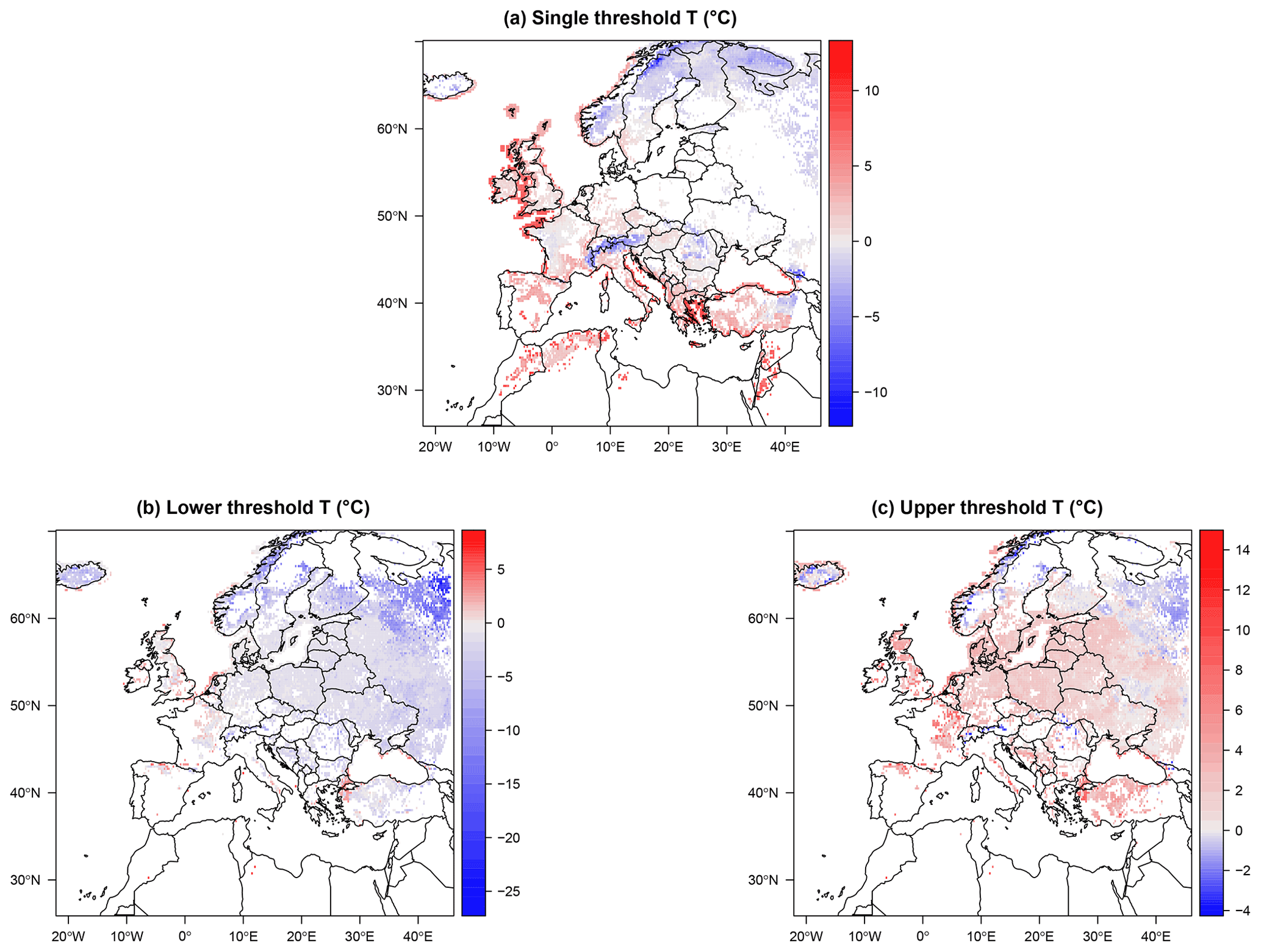
Figure 2Threshold temperatures optimized for segmented logit-linear regression, according to Eq. (A11), using ERA5 data. (a) Locations with a single threshold temperature. (b, c) Locations with double threshold temperatures, with lower thresholds (b) and upper thresholds (c) also shown.
Figure 2a displays the locations and temperature values where only one threshold is found. These are also likely locations where the choice of a STM may produce good results. However, it is clear from the figure that the values of the threshold are quite variable, displaying negative values on some areas, as opposed to the usual choice for a STM framework. In particular, strongly negative values (up to ∘C) are found over the Alps and Scandinavia, and slightly milder but still negative values are also observed over parts of eastern Türkiye, Austria, the Czech Republic, Slovakia, Hungary, Bulgaria, Romania, and Moldova. All these areas are characterized by a large or extremely large number of snowfall events (Fig. 1b), but only the Alps and eastern Türkiye are also areas with a large average DJF snowfall. The other two regions characterized by extreme total snowfall amounts, Iceland and the coast of Norway, with the exception of the most southwestern part, are instead not represented by this single threshold configuration. Thresholds ∘C are found over central–western France and Belgium, while positive values, more typical for single threshold methods are found for the UK, Spain, southern France and Germany, peninsular Italy, and the northern parts of Morocco, Algeria, and Tunisia. Panels (b) and (c) in Fig. 2 show, respectively, and for all the remaining grid points, characterized by a double threshold. These areas include Iceland and central–eastern Europe at all latitudes, excluding the aforementioned areas characterized by single thresholds. Concerning , we observe temperatures ∘C in the UK, eastern France, and central Europe, decreasing towards negative values over more northern and eastern locations, including Iceland. A similar gradient is observed for the upper threshold , with positive temperatures over UK and most of central–eastern Europe, and values closer to 0 ∘C in southern Finland and western Russia. Areas displaying unrealistically negative values for both thresholds over Iceland, coastal Norway, and northern Russia are likely areas characterized by a steep transition and noisy data, preventing the algorithm from detecting realistic threshold values.
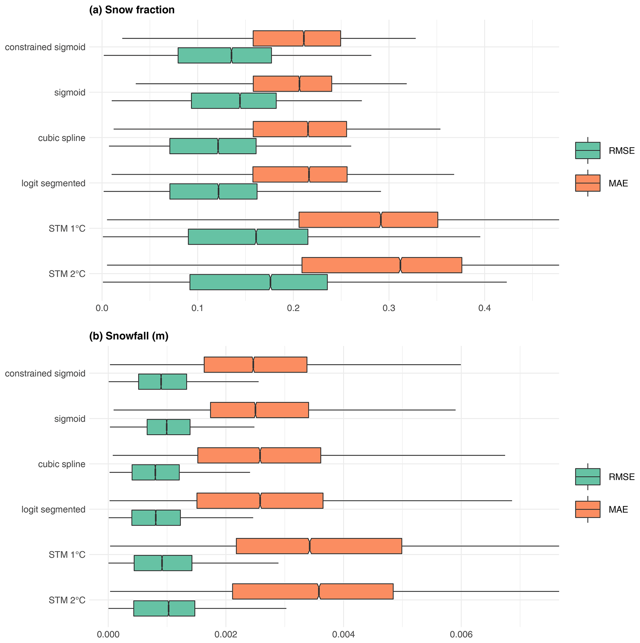
Figure 3Forecasting performance of the five considered methods applied to ERA5 reanalysis in terms of mean absolute error (orange) and root mean squared error (green). (a) Snow fraction. (b) Snowfall (m).
5.2 Statistical method evaluation and selection
We assess the performance of each method in terms of snow fraction prediction, as described in Sect. 4. For every grid point in the ERA5 dataset, we randomly split the time series of snow fraction into a training and a test set, we estimate each statistical model in the training set, and we use parameter estimates to predict the values in the test set. In Fig. 3, we show a summary of the results in terms of the chosen error measures. Each box plot refers to the values of the error measure over the entire domain for grid points with more than 30 snowfall events. The tested methods include the STM with 1 and 2 ∘C threshold temperatures, the segmented logit-linear and the cubic spline regressions, and the sigmoid fit based on NLS, both with and without constraints on the parameters. We do not display outliers in the box plot for greater graphical clarity.
We show results for both the snow fraction, directly derived from the statistical prediction (Fig. 3a), and the snowfall, obtained as (Fig. 3b).
From a visual inspection, the STM produces the poorest performance in terms of median and variability of the errors, for both fs and SF. The other methods provide very similar results, with the two versions of the sigmoid showing slightly higher median RMSE and lower median MAE; the segmented logit-linear and the cubic spline regressions display no visible differences.
In order to choose the best possible methodology based on quantitative considerations, we test for significant differences among groups using the rank test proposed by Kruskal and Wallis (1952).
We perform a total of four Kruskal–Wallis tests on snow fraction RMSE, snow fraction MAE, snowfall RMSE, and snowfall MAE. In all cases, the null hypothesis must be rejected, with virtually null p values (all , which is the smallest value resolved in R). From this, we can infer that at least one method produces significantly smaller errors compared to at least another method. However, we cannot establish exactly which groups are concerned. For this purpose, we rely on post hoc testing using the pairwise Wilcoxon rank sum test (Wilcoxon, 1992), a nonparametric alternative to pairwise Student's t tests suited for non-Gaussian samples, also known as Mann–Whitney U test. See Sect. A3 for a detailed description of the statistical tests.
For fs, the test indicates significant differences among all groups, except between spline and segmented logit-linear regressions, (p values 0.34 and 0.60 for RMSE and MAE, respectively). For SF, the test gives results analogous to fs for RMSE (no difference between spline and segmented logit-linear regressions; p value =0.20), while, in terms of MAE, differences are nonsignificant also between the two versions of STM (p value =0.56), between spline and segmented logit-linear regression (p value =0.50), between sigmoid and segmented logit-linear regression (p value =0.12), and between sigmoid fit and spline regression (p value =0.34). It is worth mentioning that, due to the very large sample size, the tests may be sensitive even to very small differences, possibly leading to a high probability of rejection, even with differences that are unrecognizable in practice.
The close similarity of results from the segmented logit-linear and the spline regression is also evident from the summary statistics of the distributions of the two error measures for the two variables, as shown in Table 1. Based on these results, spline regression seems to be potentially the best candidate, as it shows the lowest error statistics, while being less demanding than segmented regression, as it does not require the breakpoint analysis step, which is the longest and most computationally intensive step among the presented procedures.
Table 1Summary statistics of the distributions of the RMSE and MAE for snow fraction and snowfall in ERA5. The mean, standard deviations, median, and interquartile range are shown.

Table 2Summary statistics of the distributions of correlation between ERA5 reanalysis and predicted snow fraction. Note: IQR indicates the amplitude of the interquartile range.
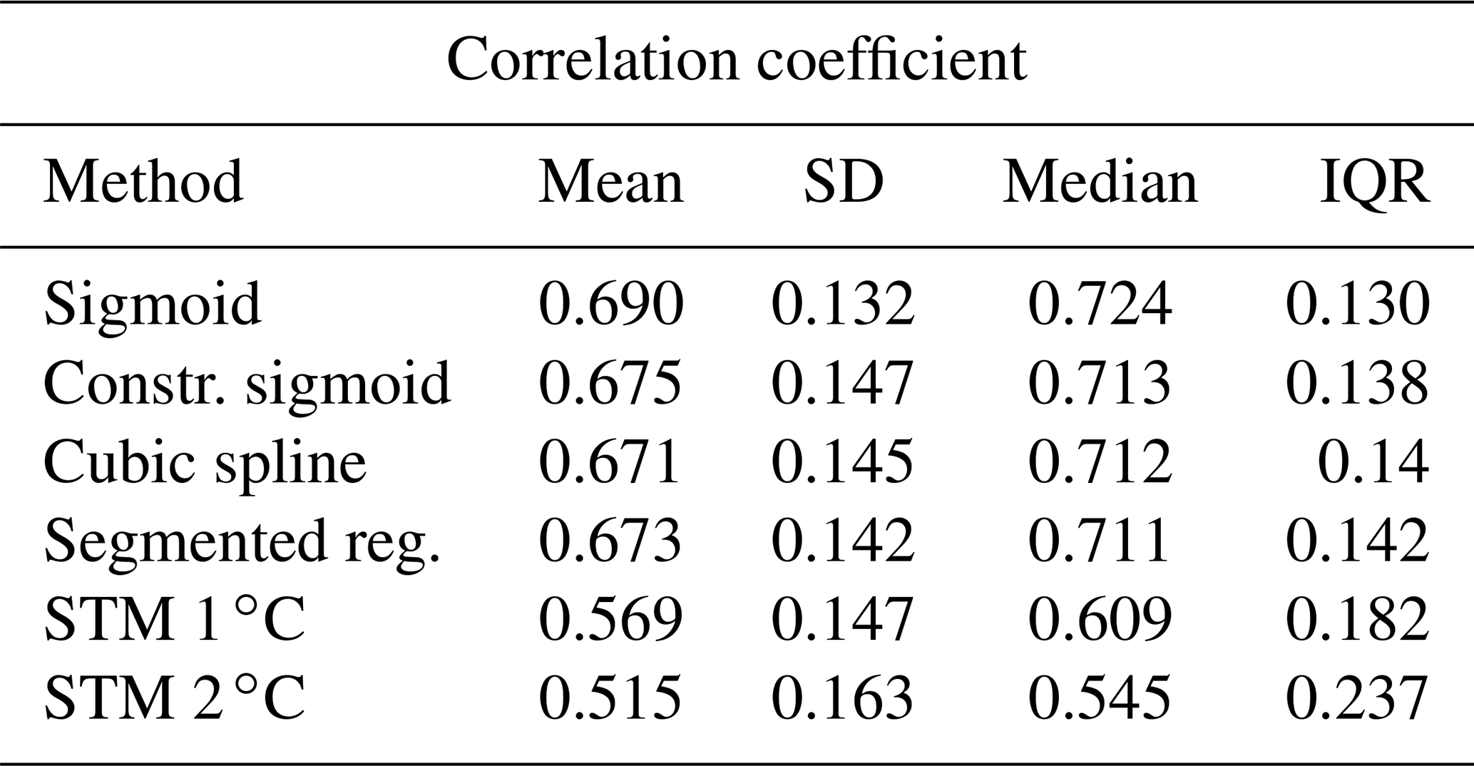
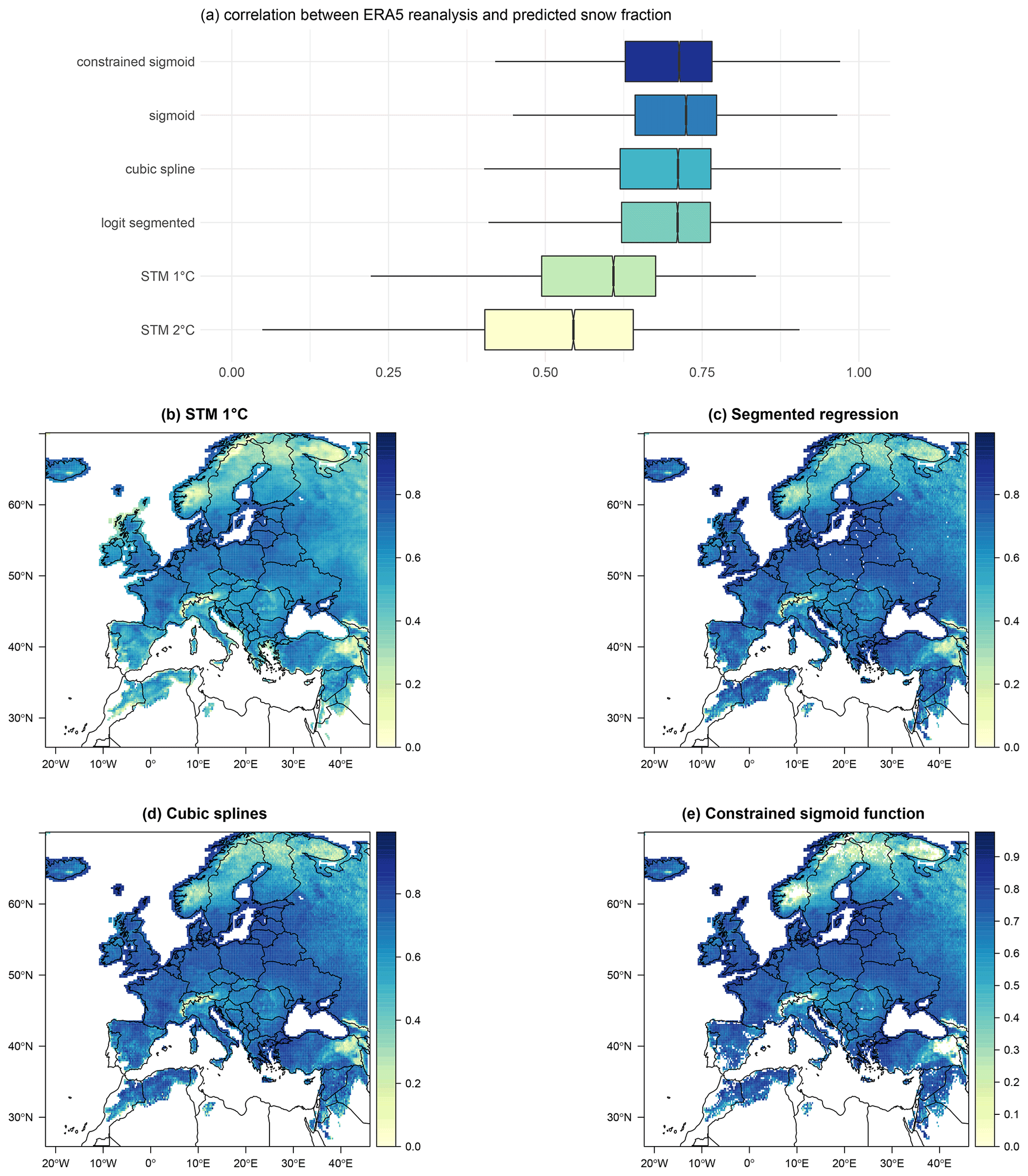
Figure 4Box plots of correlation coefficients between the ERA5 reanalysis and predicted snow fraction, using the five selected methods, for all grid points with at least 30 snowfall events (a). Mapped values of the snowfall correlation coefficient for the STM (b), segmented logit-linear regression (c), cubic spline regression (d), and constrained sigmoid fit (e). White areas over Scandinavia, the Alps, Türkiye and isolated points in Spain, southern France, and Italy shown in panel (e) are due to the non-convergence of the constrained sigmoid fit.
As a further criterion to choose the best-performing method, we consider the Pearson's correlation coefficient computed, at each grid point, between the snow fraction observed in ERA5 and predicted using the five methods under investigation. Notice that the factor linking fs and SF is for both true reanalysis and reconstructed data, so that results in terms of the correlation coefficient are exactly the same for both variables. The summary statistics for the correlation coefficient are shown in Table 2. The box plots, shown in Fig. 4a and constructed as described for MAE and RMSE, show that the STM with 2 ∘C displays the lowest correlation, followed by the 1 ∘C STM, segmented logit-linear regression, spline regression, constrained sigmoid, and unconstrained sigmoid fit. As in the previous case, the Kruskal–Wallis test finds a significant stochastic dominance of at least one group on the others, but the pairwise Mann–Whitney test suggests significant differences among all methods, except between segmented and spline regression (p value 0.9985).
Figure 4b–e show the spatial structure of correlation between predicted and observed snow fraction for all methods, except the STM with 2 ∘C threshold and the constrained sigmoid. Clearly, areas characterized by frequent and abundant winter snowfall, such as the Alps, Scandinavia, and eastern Türkiye, correspond to the lowest values of the correlation coefficient. It becomes evident that the slightly better performance of the unconstrained sigmoid fit is due to the non-convergence of the NLS algorithm over parts of the Alps, Norway, Sweden, Finland, and northern Russia, which are characterized by the lowest correlation values. This suggest that, while this method can perform as well as the segmented and spline regressions, it may be sensitive to misspecification, making it unsuitable for areas where the transition departs from an inverse S-shaped function. The constrained version does indeed show better convergence as it providing results very close to the logit-linear segmented and cubic spline regression.
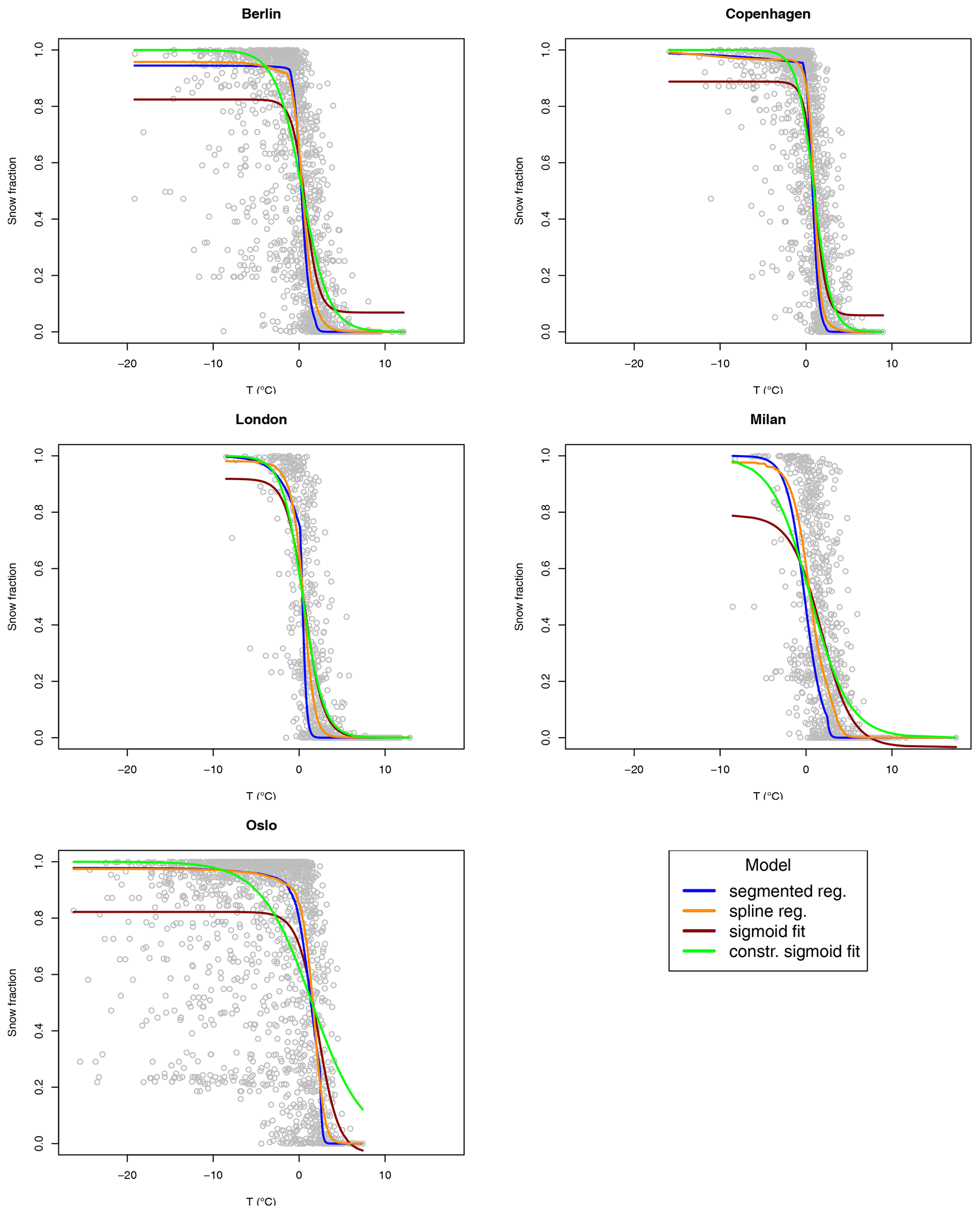
Figure 5Snow fraction as a function of temperature for the five ERA5 grid points closest to some European cities (gray circles). Solid lines represent fitted values for the segmented logit-linear regression (blue), spline regression (orange), sigmoid fit (dark red), and constrained sigmoid fit (green).

Figure 6Snow fraction as a function of temperature for the five ERA5 grid points closest to some European cities (gray circles). Solid lines represent fitted values for the segmented logit-linear regression (blue), spline regression (orange), sigmoid fit (dark red), and constrained sigmoid fit (green).
Figures 5 and 6 show the transition for a total of 10 locations corresponding to the closest grid points to some European capitals and the fits resulting from the segmented logit-linear regression, spline regression, and sigmoid fit, which are both constrained and unconstrained.
It is clear that the unconstrained sigmoid fit has some issues with extreme values of fs, especially in catching the saturation at fs=1 for very low values of T. The constrained version of the sigmoid fit is well-behaved at the extremes of the transition; however, in most of the shown locations, it is less accurate than the logit-linear segmented and cubic spline regression in following the overall transition.
As expected, fitted values from segmented and spline regressions are quite close, with the splines giving the smoothest result, since they are continuous at the knots by construction.
It is clear that, overall, the segmented logit-linear regression and the spline regression perform significantly better at reconstructing the snowfall compared to the STM. However, these results do not constitute strong evidence towards a better performance in reconstructing snowfall in practical cases, i.e., when it is unobserved or severely biased. To this purpose, we will apply both methods to reconstruct the snowfall in a climate projection model, and we assess which one produces the least biased snowfall using bias-adjusted temperature and precipitation as an input.
As an additional element to evaluate the performance of the identified methods, we assess if they can produce robust snowfall estimates in a pseudo climate change scenario. In order to do so, we repeat the validation procedure described in Sect. 4; after ordering the ERA5 dataset based on the annual DJF average temperature, we take the coldest 25 % as the training set and the warmest 25 % as the test set. We run this procedure for all methods, except the 2 ∘C STM, which clearly showed the poorest performance and will not be considered again in the following.

Figure 7Performance of the statistical methods for the prediction of snow fraction, trained on the 25 % coldest ERA5 years, in forecasting in the 25 % warmest years. (a–e) Maps of Pearson's correlation coefficient between prediction and reanalysis. (f, g) Comparison of the box plots of the correlation coefficient and of the statistical method performance in terms of RMSE and MAE, respectively. White points over northern Europe and Russia indicate non-convergence of the two sigmoid fits.
Figure 7 shows the statistical model performance metrics in analogy with Figs. 3 and 4. Figure 7a–e display the map of the event-to-event correlation coefficient, showing overall higher values than for the random training and test sets, which is arguably due to more frequent snowfall in the top 25 % coldest years providing more training data. On the other hand, both versions of the sigmoid fit exhibit convergence problems over a larger number of grid points, despite still being limited to the Alps, Scandinavia, and Russia, with the worst performance provided by the unconstrained fit.
Similar to the case of randomly drawn train and test sets, the STM shows the lowest correlations, followed by the segmented logit-linear and spline regressions, as shown by the box plot in Fig. 7f. The sigmoid fits display less variability in the lower tail of the box plot, probably thanks to the less dramatic lowering in correlation over western France, especially when compared to the spline regression. The performance in terms of RMSE and MAE (Fig. 7g) is also comparable to the random train and test sets case, with cubic splines performing the best.
Overall, assuming that separating cold and warm years can be a proxy of climate change to assess statistical model performance, the two regressions perform very similarly to the general case in terms of forecasting error, without any visible improvement or decrease in accuracy. As expected, the STM has the worst performance, while the sigmoid fit could present advantages over some areas but more pronounced convergence problems where DJF precipitation mainly falls as snow. However, we observe an improvement in the correlation between predicted and true forecasting values. We argue that this effect is likely due to precipitation patterns in years characterized by extreme temperatures in the historical period, and it should not be expected to happen under future climate change.
5.3 Bias correction of climate simulations
We now assess the performance of the considered methods on the output of the IPSL_WRF climate simulations for the period 1979–2005. For this RCM, we have near-surface temperature and total daily precipitation bias-corrected using CDF-t with respect to ERA5. However, available snowfall data are not corrected, and this presents non-negligible differences compared to ERA5 in terms of both the long run statistics and probability distribution of daily snowfall.
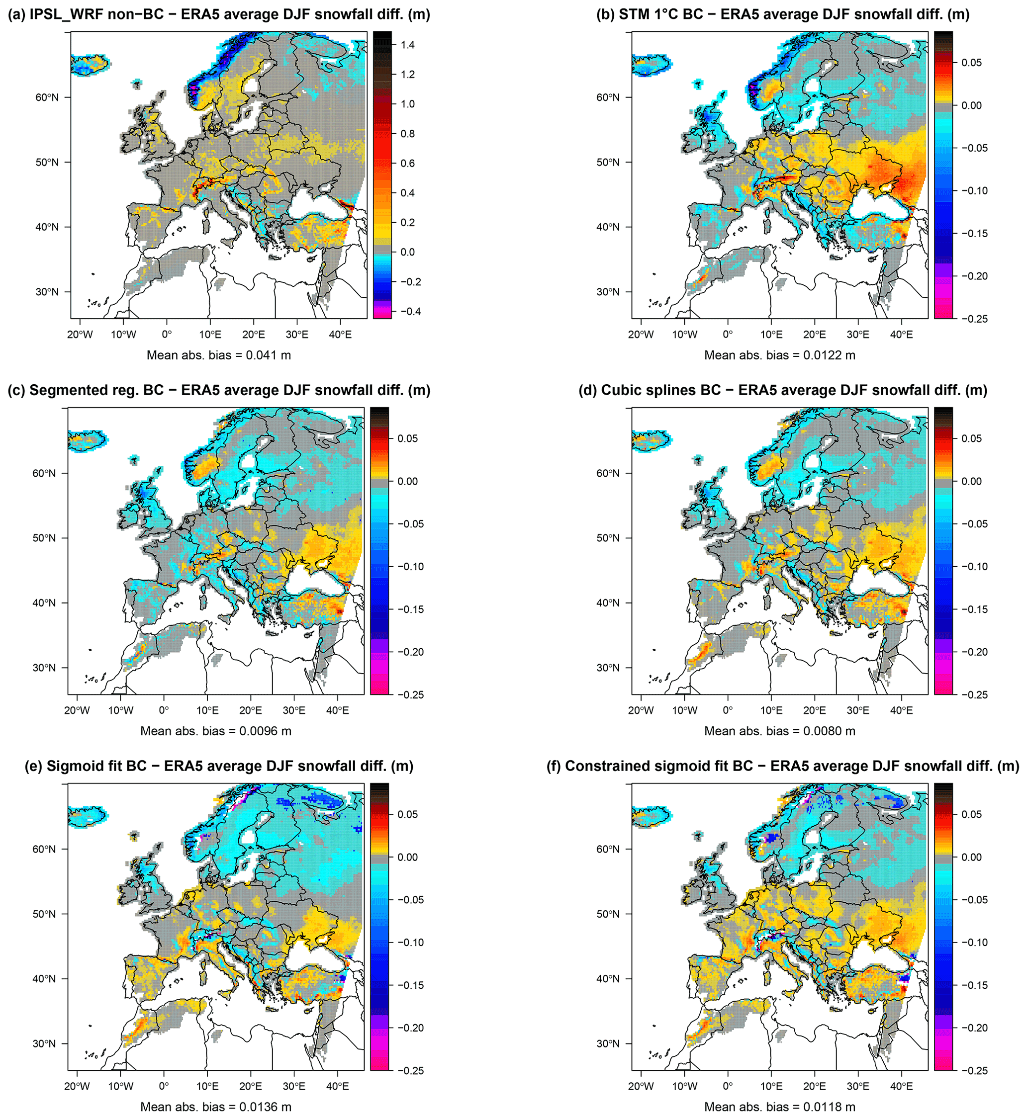
Figure 8Difference in meters between the statistical approximation and reanalysis average of DJF snowfall for the years 1979–2005. The IPSL_WRF model (a), 1 ∘C STM (b), segmented logit-linear regression (c), cubic spline regression (d), unconstrained (e), and constrained sigmoid function (f) are shown.
Figure 8 shows the differences in average DJF snowfall between IPSL_WRF and ERA5 and between each statistical method and ERA5. The RCM displays larger biases compared to the statistical methods, especially the positive values over the Alps and negative bias over the coast of Norway and, with smaller values, over western Iceland, the Balkans, and northern Russia. Overall, all methods produce a decrease in snowfall bias, including the STM.
It is also worth noting the different spatial distribution of the bias sign, depending on the method. The two versions of the sigmoid fit are the only methods that avoid the positive bias patch over Norway; however, the unconstrained sigmoid is characterized by larger areas of negative bias between Scandinavia and Russia, while the constrained version produces more positively biased values over central Europe.
To assess the overall performance of the models, we compute the mean absolute bias as the spatial mean of the absolute differences between modeled and ERA5 DJF snowfall differences. The cubic splines produce the smallest bias (0.008 m), followed by segmented regression (0.0096 m), constrained sigmoid (0.0118 m), STM (0.0122 m), unconstrained sigmoid (0.0136 m), and non-bias-corrected IPSL_WRF (0.041 m).
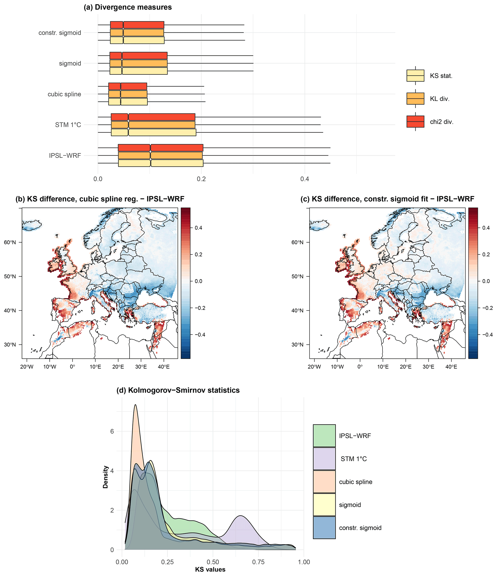
Figure 9Performance of the statistical methods as bias correction methods of snowfall in terms of statistical divergences. Divergence measures box plots for statistical methods and raw IPSL_WRF simulations (a). Maps of KS statistical differences between IPSL_WRF and spline regression (b) and constrained sigmoid fit (c). Comparison of the probability density function of the KS statistics associated with the four considered statistical methods and the uncorrected IPSL_WRF model (d).
We evaluate the performance of the STM, cubic spline regression, and the two versions of the sigmoid fit and compare it to the values produced by the IPSL_WRF model, using three measures of proximity between probability distributions of SF, as described in Sect. 4 (KS, KL, χ2). At each grid point, we estimate the three divergence measures between the empirical probability distribution of ERA5 and of each statistical method. We do not consider the segmented logit-linear regression, since results produced by such a method are almost identical to the ones obtained using spline regression, but require also the breakpoint analysis, which is a lengthy and computationally expensive step for large datasets, making it a less attractive candidate.
The results are summarized in Fig. 9a through the box plots of the values considering the entire domain. Outliers are excluded for greater graphical clarity. For each method, the three divergence measures assume similar values overall. All methods to approximate snowfall produce smaller values of the statistical divergences compared to the raw IPSL_WRF output. The largest dissimilarity is observed for the STM: as already mentioned, such a method can be expected to produce accurate snowfall climatologies, but the resulting SF distributions cannot be realistic, given the binary partition.
The spline regression appears to be the best method in terms of both median and variability, as it consistently displays the smallest interquartile range (IQR) for all the three measures. However, while χ2 and KL produce very homogeneous values over the domain (not shown), KS is more spatially differentiated and also has larger outlier values. Figure 9b and c show the spatial distribution of the difference between IPSL_WRF KS distance compared to cubic spline regression and constrained sigmoid fit, respectively. Both methods display a clear spatial coherence, showing that improvements in terms of KS statistics concern central and eastern Europe, especially below 45∘ latitude. Figure 9d shows the distributions of the KS distance for the IPSL_WRF and the four discussed methods. Once again, smallest values are observed for the cubic spline that appears to be the best-performing method when considering the domain as a whole. Almost no difference is found between the constrained and the unconstrained version of the sigmoid fit.
5.3.1 Regional extremes
The results discussed so far show that the IPSL_WRF model is affected by a spatially inhomogeneous and sometimes important bias, and that the snowfall reconstruction based on the methods selected in Sect. 5.2 produces more realistic values on the majority of grid points. In particular, the greatest advantage seems to be in very snowy areas, such as the Alps and Norway, where post-correction biases are comparable to the rest of the domain, while those in the IPSL_WRF model are roughly up to an order of magnitude larger. Other areas, such as central Europe, are characterized by smaller biases, even in the raw climate model output and in the STM. In this paragraph, we focus our analysis over limited areas with high (the Alps and Norway) and low (France and Germany) bias. Here, we only show results for the constrained version of the sigmoid function. We define the Alps region based on Eurostat 2016 nomenclature of territorial units for statistics (NUTS 3), choosing provinces belonging to France, Switzerland, Italy, and Austria characterized by large values of total 1979–2005 snowfall and large differences between ERA5 and IPSL_WRF. In particular, we include the regions marked by the NUTS 3 codes listed in Table A1.

Figure 10Maps of average 1979–2005 DJF snow differences over the Alps region between raw IPSL_WRF (a), STM (b), cubic spline regression (c), sigmoid fit (d) bias correction, and ERA5. Corresponding summary box plots are shown in panel (e).
The IPSL_WRF simulation is characterized by a large positive bias over the Alps, with values up to ∼1 m difference in the average 1979–2005 DJF snowfall, as shown in Fig. 10a. Figure 10b–d clearly show the dramatic reduction in the bias for all the statistical methods, with values decreasing from ∼0.5–1 to ∼0.05 m especially in the most affected areas of the central–western Alps. As already mentioned, however, the sigmoid fit does not converge over several grid points over the Alps, making this method not suitable for snowfall reconstruction over this region.
Overall, the median bias of the STM and spline regression remains slightly positive, but the IQR of the differences with respect to ERA5 is reduced by around an order of magnitude, as evident from Fig. 10e. The overall best performance in terms of average DJF snowfall is shown by the spline regression, with both the smallest residual bias and variability.
Since comparing IPSL_WRF and its adjusted versions to ERA5 does not provide a one-on-one correspondence between snowfall events, it is not possible to compute correlation coefficients between reanalysis and statistically reconstructed snowfall time series at each grid point as in Fig. 4. Instead, we can study the correlation between the total 1979–2005 ERA5 snowfall and the total 1979–2005 snowfall simulated by IPSL_WRF and approximated with the STM, cubic spline regression, and sigmoid fit at each grid point.
The upper left quadrant of Table 3 reports values of the intercept and slope of the least squares line plus the determination coefficient; the asterisks mark coefficients that are significantly different from 0 at the 5 % level. The slope estimate is accompanied by its 95 % confidence interval, obtained as ±2 s.e., where s.e. is the standard error.
In case of an ideal bias correction method, differences between the reference dataset and corrected model output would be a sequence of uncorrelated zero-mean Gaussian random variables. This implies a linear relationship with zero (nonsignificant) intercept, a significant slope close to 1 (i.e., with 1 included in the confidence interval), and an R2 as close to 1 as possible. The intercept of the IPSL_WRF is significant and negative, the slope is significantly different from 1, and a determination coefficient is R2=0.73. All the statistical methods produce a remarkable improvement in the parameters, with the cubic spline regression displaying the values closest to the ideal case. These results demonstrate a marked improvement of the long run snowfall statistics over the Alps obtained with any of the considered statistical approximations, compared to the uncorrected climate model snowfall.
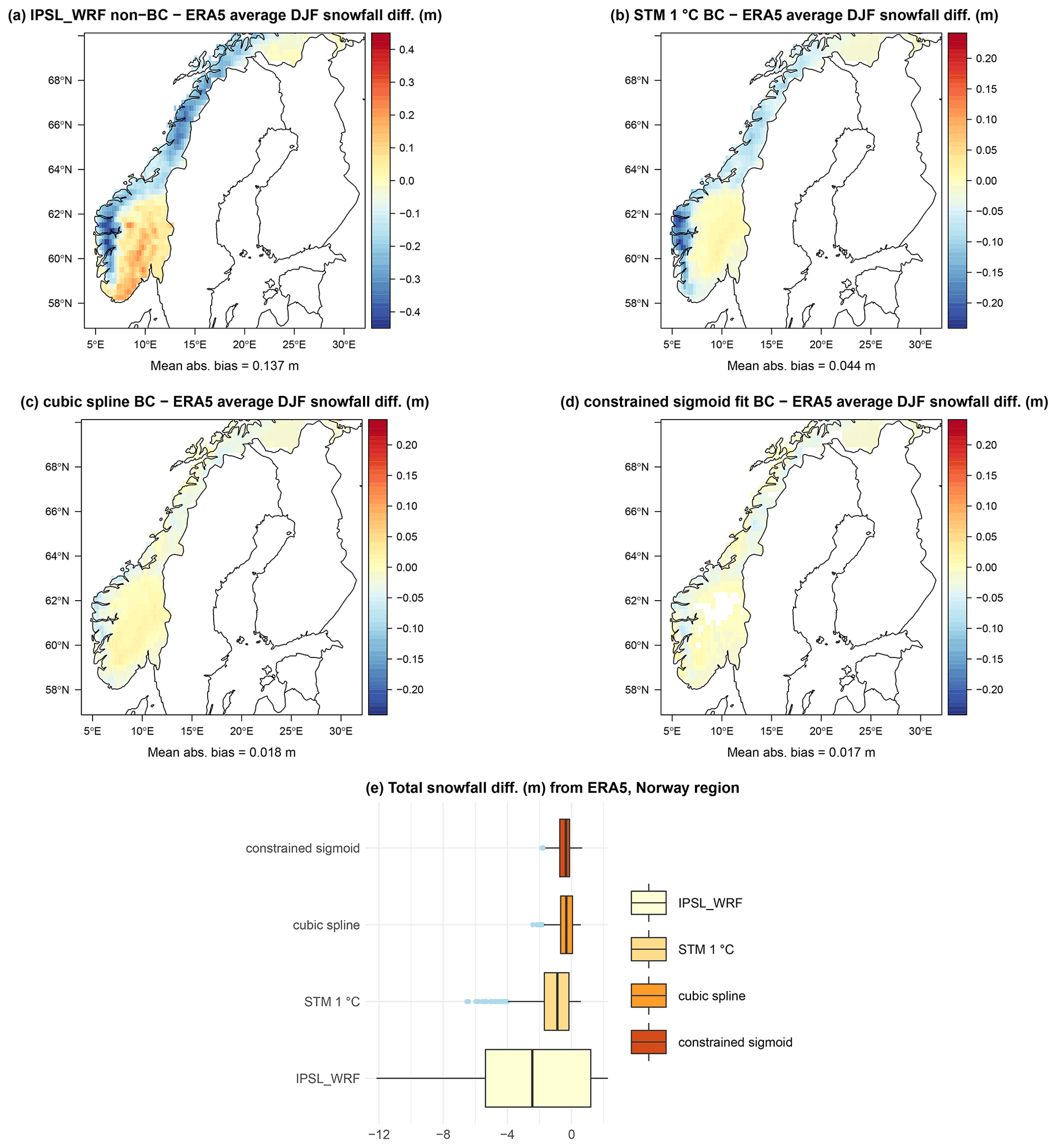
Figure 11Maps of average 1979–2005 DJF snow differences over Norway between raw IPSL_WRF (a), STM (b), cubic spline regression (c), sigmoid fit (d) bias correction, and ERA5. Corresponding summary box plots are shown in panel (e).
We repeat the same analysis for Norway, another area where DJF snowfall constitutes a large proportion of total DJF precipitation and the IPSL_WRF model shows large biases. As shown by Fig. 11a, IPSL_WRF presents a negative bias, up to −0.4 m on average for 1979–2005 DJF snowfall, on the entire western and northern sides of the country, and positive biases up to m on the southern areas, making snowfall over one of the most snowy areas in Europe heavily misrepresented. Again, Fig. 11b, c, and d show the reconstructed snowfall using STM, cubic spline regression, and constrained sigmoid fit, respectively. In this case, the bias pattern is still persistent after correction, with the exception of a passage from positive to negative values over the southern coast. The magnitude of the residual bias is reduced by a factor ranging from ∼2 for the STM to ∼5 for the spline regression and sigmoid fit, compared to IPSL_WRF. As for the Alps, the box plots of total snowfall over the country, shown in Fig. 11e, suggest that the best performance in terms of correction of average DJF snowfall is obtained using the cubic spline regression and by the sigmoid fit, without large differences between the two methods. However, while the mean absolute bias is similar for cubic splines and the sigmoid fit, the latter results in an area of non-convergence in a region characterized by large DJF snowfall totals. As for the Alps region, STM estimates are less biased compared to the raw IPSL_WRF output, even though its performance is less close to the one of the two other competing methods.
As shown in Table 3, the relationship between total DJF snowfall simulated by the IPSL_WRF model and ERA5 is characterized by poor correlation (R2=0.12) and regression parameters. Snowfall reconstruction via statistical methods produces, once again, a sizable improvement in snowfall estimation, with R2=0.91 for the STM and R2≥0.98 for the cubic splines and sigmoid fit.

Figure 12Maps of average 1979–2005 DJF snow differences over France between raw IPSL_WRF (a), STM (b), cubic spline regression (c), sigmoid fit (d) bias correction, and ERA5. Corresponding summary box plots are shown in panel (e).
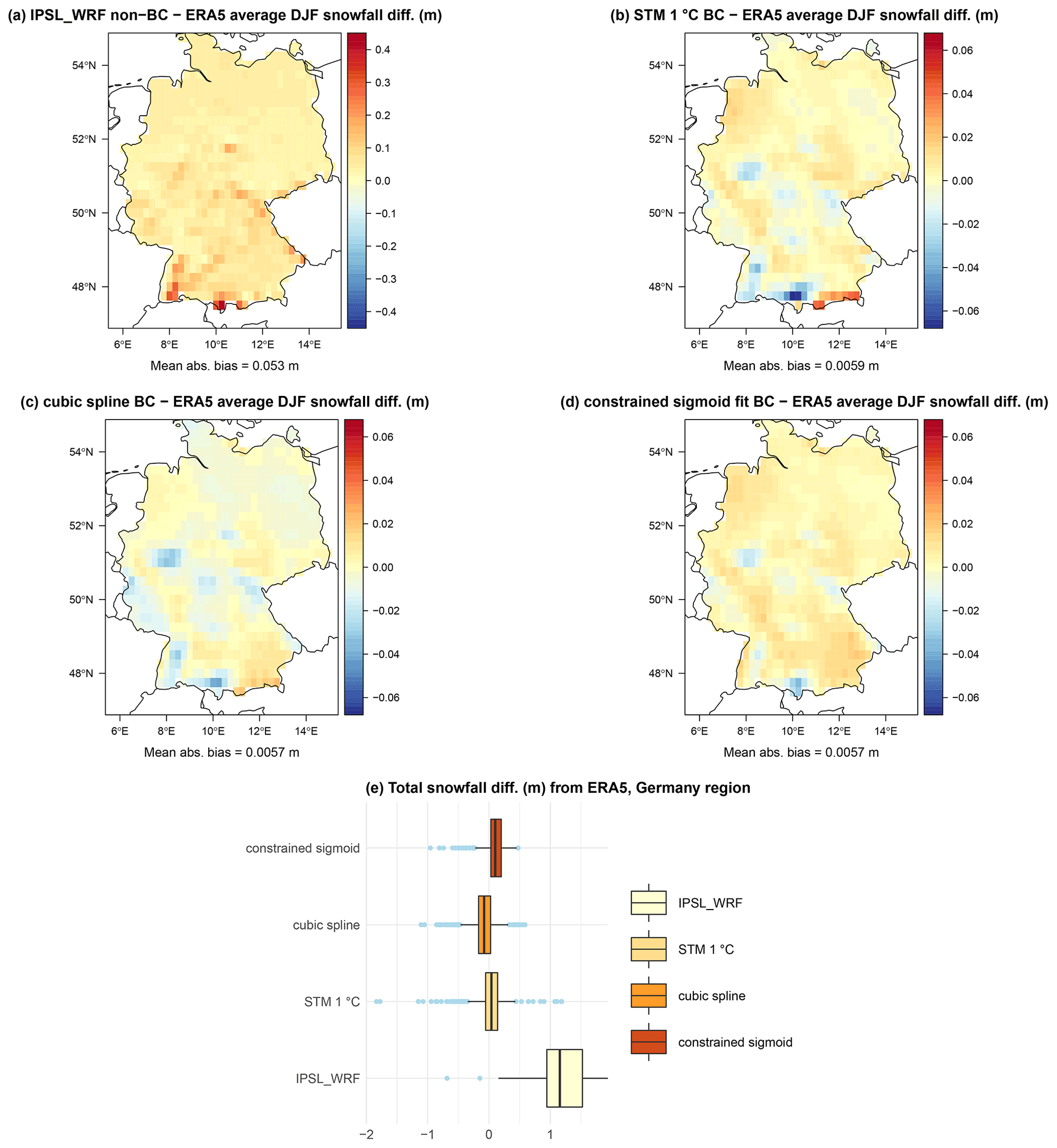
Figure 13Maps of average 1979–2005 DJF snow differences over Germany between raw IPSL_WRF (a), STM (b), cubic spline regression (c), sigmoid fit (d) bias correction, and ERA5. Corresponding summary box plots are shown in panel (e).
Both Norway and the Alps regions are characterized by mountain ranges subject to orographic forcing of moist air masses and by low DJF temperatures due to elevation (especially for the Alps) and latitude (Norway). Moreover, all methods show the lowest correlation between observed and reconstructed snowfall in the validation phase over these areas (see Fig. 4). We now repeat the same assessment for areas where snowfall is overall less abundant and driven by different mechanisms, and the statistical methods show higher correlations in the validation phase. Figure 12 shows results for France and Fig. 13 for Germany. Both countries are characterized by nonhomogeneous orography, continental areas, and coasts directly influenced by the Atlantic Ocean, the North Sea, and the Mediterranean Sea. In both cases, the IPSL_WRF bias is overall positive but smaller compared to the previously analyzed regions, with the largest values in the areas closest to the Alps region. In terms of average DJF snowfall (Figs. 12e and 13e), all three statistical models produce a visible improvement compared to the raw climate model, with some residual biases especially over the more elevated areas. Differences among models over these two areas appear to be negligible.
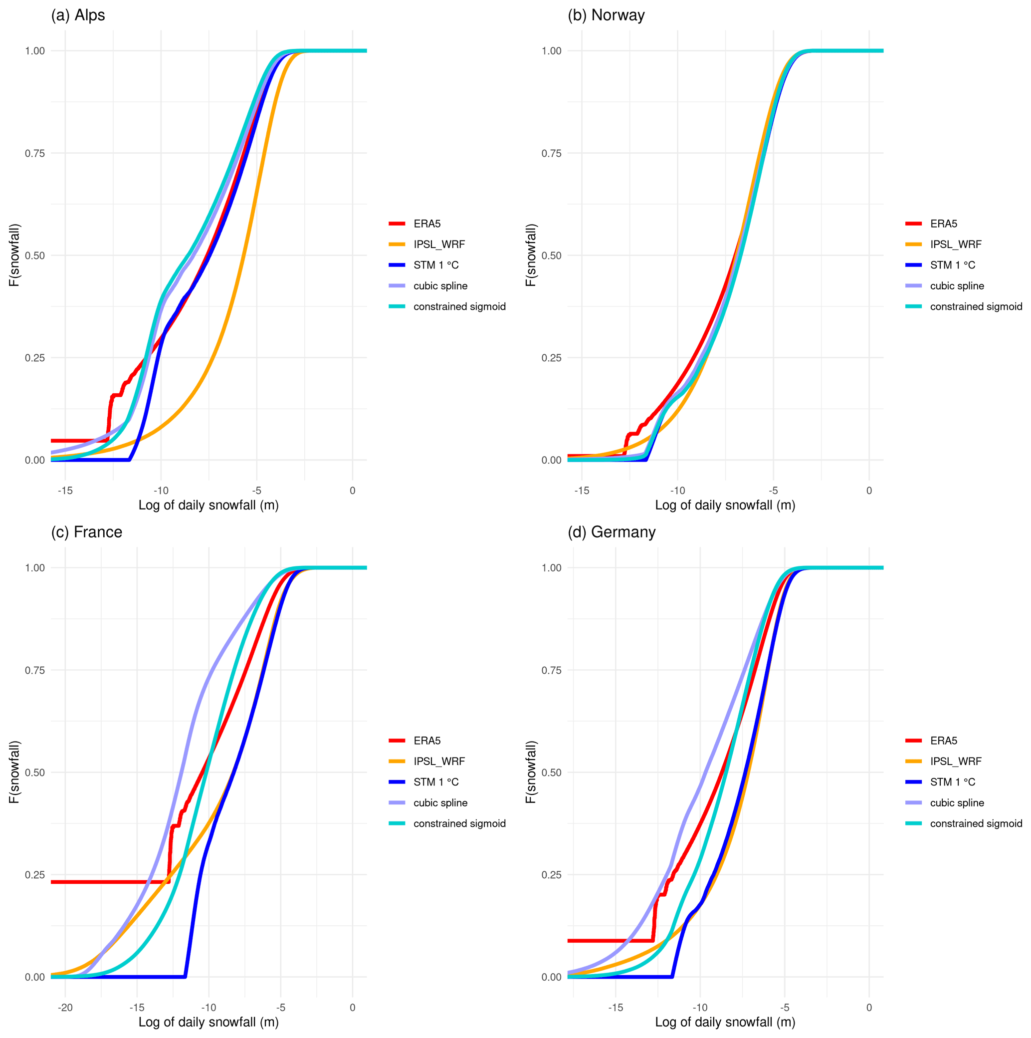
Figure 14Comparison between cumulative distribution function of daily snowfall in ERA5 reanalysis (red lines), raw IPSL_WRF model output (orange line), STM (blue line), cubic spline (purple line), and constrained sigmoid (turquoise line) bias correction for (a) the Alps, (b) Norway, (c) France, and (d) Germany. The distributions are shown in a natural logarithmic scale to magnify the differences.
As already mentioned, bias adjustment usually aims at correcting as much of the distribution of the observable as possible. To assess if and how well our methods work in this sense, we compare the empirical cumulative distribution function (ECDF) of daily snowfall, once again considering each region as homogeneous. Figure 14 shows the comparisons among the ECDFs with a logarithmic x axis to magnify small differences. In all cases, the IPSL_WRF distribution is visibly different from the reference. For France and Germany, the STM results in distributions very similar to those of the raw model, despite the small residual biases in snowfall totals, while it approximates the ERA5 distribution very well in the case of the Alps region. The two more complex methods produce a visible improvement in all cases, compared to the raw IPSL_WRF model.
In summary, we have shown that combining a breakpoint search algorithm and a flexible regression method – be it a segmented logit-linear or a cubic spline regression – allows for a reliable snowfall reconstruction in climate simulations. This method proves to be effective both in correcting large mean biases and in preserving the shape of the entire probability distribution of (daily) snowfall rather than only long run totals. This result is crucial for studying the characteristics of future snowfall in a wide range of environments, encompassing regions characterized by frequent and abundant snowfall in cold climates and temperate areas where occasional snowstorms and heavy wet-snow events can cause serious loss and damage.
Table 3Summary statistics of the linear relationship between reconstructed and reanalysis snowfall over the Alps, Norway, France, and Germany.

* Denotes significance at the 5 % level.
We have presented four statistical methods to estimate the snowfall fraction of total DJF precipitation over Europe, provided that a reliable measure of near-surface temperature is available. This is a relevant problem in both hydrology and climatology, since an accurate estimation of snowfall is challenging in case of both observed or simulated precipitation.
In case of observational data, especially over large areas where a single weather station is not representative, snowfall is often unobserved due to difficulties in making its measurement an automated procedure. On the other hand, climate model outputs often include snowfall, but this is affected by a bias arising from the physical and mathematical approximations contained in the model scheme. For other variables such as temperature and total precipitation, we can rely on well-established and relatively simple univariate bias correction methods that can be applied pointwise in the case of gridded data. However, snowfall presents more challenges, since not only the magnitude but also the number of events is biased as a consequence of biases in the temperature. Thus, its correction would require conditioning on temperature and precipitation, and possibly including a stochastic generator of snowfall events to correct snowfall frequency, other than snowfall magnitude. Therefore, the availability of simple methods to reconstruct the snow fraction of total precipitation is a great advantage in contexts where much more complex and computationally costly procedures should be created and applied in order to obtain an accurate snowfall measurement.
The techniques applied in the existing literature mainly consist of a binary representation based on a threshold temperature, linear interpolations between two thresholds, and a binary representation outside of the inter-threshold interval or fitting parametric S-shaped functions with nonlinear least squares. The simple binary description is effective in its simplicity when the researcher is interested in particular in extreme events or long run total climatologies, but it cannot provide a reliable reproduction of the entire snowfall distribution. Moreover, the thresholds in the first two methods are often established simply by visual inspection of the plot of snow fraction against temperature, or analyzing the entire available dataset at once. However, in the case of gridded data over large areas, the optimal threshold values may vary, depending on the location.
The first considered method consists of a binary partition (STM), testing two possible thresholds at 1 and 2 ∘C. For our domain, the 1 ∘C proved to provide better results compared to the alternative.
The second method is a segmented linear regression on the logit of the snowfall fraction, informed about the location-specific optimal number of thresholds (between 0 and 2) via a breakpoint search algorithm.
As a more flexible alternative to segmented logit-linear regression, we introduced a nonlinear regression based on cubic splines, where the spline knots are taken as the deciles of the location-specific temperature distribution. This allows us to construct a flexible statistical model without requiring computationally intensive additional step such as the breakpoint search in the case of the segmented logit-linear regression.
Finally, we adopt a parametric nonlinear statistical model, in which the link between near-surface temperature and snow fraction is given by a hyperbolic tangent function, whose parameters are estimated via nonlinear least squares.
We used ERA5 reanalysis over Europe for the period 1979–2005 for validation, by estimating each statistical model at each grid point over a training set and comparing the performances in terms of prediction of out-of-sample values. In this validation phase, the STM provides much less accurate prediction compared to the more complex methods. The results obtained with the two regression models are very similar; however, the longer, computationally intense, and more complex procedure required to inform the segmented logit-linear regression makes it less advantageous compared to the spline regression. Finally, the constrained sigmoid fit produces results comparable overall to the spline regression over most grid points. However, it seems to be slightly less flexible than its competitors, as the fit can fail to converge over areas where DJF precipitation mainly falls as snow, such as Scandinavia and the Alps, or be negatively affected by outliers, as seen in the transition curve for Oslo. Based on our result, we conclude that this method could be superior to others for studies conducted over limited areas characterized by very smooth snow transitions. However, it does not seem to be adequate for studies over very large domains or when using already validated and published datasets that could still contain some noisy data, as is the case for snowfall in ERA5.
Results hold when using the 25 % coldest and warmest years as training and test sets, respectively. This observation is encouraging in view of the application of the analyzed techniques to study snowfall under different climate projection scenarios, provided that the performance can be reproduced when considering climate simulations instead of reanalysis.
To tackle this question, we consider the historical period of 1979–2005 in the IPSL_WRF high-resolution climate simulation model, for which bias-corrected near-surface temperature and total precipitation are available, while snowfall is not adjusted, showing very large biases with respect to ERA5, especially over areas characterized by frequent and abundant snowfall. We find that the point-specific estimates obtained in the model selection phase can be applied to this dataset to obtain snowfall estimates much closer to reanalysis compared to the raw IPSL_WRF data. We exclude the segmented logit-linear regression, since its performance did not show differences compared to the spline regression, making its higher complexity not justified.
We validate our results by both considering the entire domain and specific regions. We find that, in general, the reconstructed snowfall improves remarkably in terms of long run statistics and similarly between probability distributions with all methods, proving that they can be used in place of more complex multivariate bias correction schemes. However, it is clear that the best method depends on both the geographical area and the objective. For example, over the Alps, the best performance is given by the spline regression both in terms of average DJF snowfall bias and distribution of daily snowfall events but without dramatic differences among the three methods; over Norway, another region characterized by large DJF snowfall, the STM performs discernibly worse than the other two methods in terms of average snowfall, but it produces the best bias correction of the daily snowfall distribution, even though with no dramatic differences compared to the spline regression and sigmoid fit. For areas such as France and Germany, the STM is competitive against more complex methods in terms of both snowfall averages and daily snowfall distribution.
Overall, among the tested methods, we discard the segmented logit-linear regression, which requires a time-consuming step to perform breakpoint analysis over the grid and without performing better than its competitors. We remark that, to reproduce average DJF snowfall, the simple STM can be applied with success; however, unlike what is reported in Faranda (2020), its performance is sensitive to the choice of the threshold temperature, as we find that a value of 1 ∘C improves snowfall reconstruction compared to 2 ∘C, in line with Jennings et al. (2018). In some areas, such as Germany, the sigmoid fit produces the best results, but it can be a poor choice to approximate the snowfall fraction over areas where most precipitation falls as snow in the considered season. Overall, we find that the cubic spline regression with knots given by temperature quantiles (deciles in our case) has the best tradeoff between feasibility and accuracy of results. However, for studies over limited areas, it could be worth comparing different specifications (e.g., STM, spline regression, and a sigmoid fit) on reanalysis or observations, to establish which techniques produce the most accurate results.
Limitations
We also clarify some of the limitations of our analysis. The nature of climate datasets makes multiple comparisons among methods and BC techniques very demanding in terms of data storage and computational time. For this reason, we limited our analysis to one reanalysis dataset (ERA5), one marginal bias correction technique (CDF-t), one climate projection model (IPSL_WRF), and to the DJF season.
We do not consider the choice of ERA5 problematic with respect to other gridded datasets that could be observational (e.g., E-OBSv20) or other reanalysis (e.g., NCEP/NCAR). While the actual values could change between datasets, we do not foresee this directly affecting the performance of the methodology we presented in terms of improvement of the raw simulations with respect the chosen reference dataset.
On the other hand, the choice of the BC may influence the outcome of our statistical modeling procedure. The CDF-t is applied marginally to each variable, so that there is no guarantee that the inter-variable correlations are correctly reproduced in the bias-corrected climate model output. Indeed, Meyer et al. (2019) showed that applying multivariate as opposed to univariate BC produces significant changes in estimated snow accumulation, stressing the importance of modeling the interdependence between precipitation and air temperature in hydrological studies focused on snowy areas. The choice of the BC, in general, should be tuned on the tradeoff between complexity and need for controlling specific feature, in this case the inter-variable correlation. In our case, we considered a climate dataset prepared in the context of the CORDEX-Adjust project, which is made available already adjusted with respect to ERA5 using marginal CDF-t. Our results show an improvement in snowfall representation even relying on marginal BC; however, we stress that the methodology should be validated again if used on datasets prepared with different BC techniques to assess whether this difference affects the predicting performance of the statistical method.
On the same note, we remark that prediction accuracy may vary across different climate models, due to the different physical approximations and parameterizations, which are likely to affect the relationship between near-surface temperature and precipitation. Due to these differences, even other RCMs from the EURO-CORDEX project may exhibit variability in the performance of the snowfall reconstruction. This holds true for all statistical methods cited in Sect. 1, as it is rarely the case that snowfall reconstruction techniques are tested over an ensemble of different climate models. Once more, we stress the importance of assessing the performance of the chosen methodology to approximate snow (or compare several of incidences thereof) by validating it on the historical period of the available climate models in reference to the available reanalysis/observation dataset.
We have presented four statistical methods to estimate the snowfall fraction of total precipitation, provided that a reliable measure of near-surface temperature is available. This is a relevant problem in both hydrology and climatology, since an accurate estimation of snowfall is challenging in the case of both observed or simulated precipitation.
There are two methods, namely the segmented logit-linear and the spline regressions, that are an extension of traditional precipitation-phase partitioning methods based on estimating the snowfall fraction of total precipitation on the base of one or multiple threshold temperatures. For the segmented logit-linear regression, we estimate the number of such thresholds by means of a breakpoint search algorithm, while splines do not require the specification of physically meaningful thresholds, and quantiles of the temperature can be assumed as knots. The other two methods, i.e., STM and sigmoid fit, are used in studies already present in the literature, even though not with the scope of eliminating biases in climate simulations.
The two regression models perform the best in terms of prediction error and correlation between real and reconstructed values in a train–test sets validation framework, based on the ERA5 reanalysis dataset. These two methods also show robustness with respect to possible non-stationarity, when choosing the 25 % coldest years as training set and the 25 % warmest years for testing. In this context, the sigmoid fit also produces good results, but it could fail in case the snow fraction transition curve is not well represented by an S-shaped function.
When applied to reconstructing snowfall in a regional circulation climate model, all techniques produce results with a markedly reduced bias respect to ERA5, when compared to raw climate model simulations.
We conclude that statistical methods based on spline regression and sigmoid fit, informed by bias-corrected temperature and precipitation, are capable of providing a reliable reconstruction of snowfall that can replace more complex bias correction techniques, with better performances than similar methods based on parametric assumptions or binary phase separation. For limited areas, and depending on the task, simpler single threshold methods can perform equally well and could be advantageous in case fast or computationally light procedures are needed.
A1 Breakpoint analysis and segmented logit-linear regression
In order to estimate the temperature thresholds, we rely on breakpoint analysis. This method was originally developed by Bai (1994) to detect and date a structural change in a linear time series model and later extended to the case of a time series with multiple structural breaks (Bai and Perron, 1998). The technique was further generalized by Bai and Perron (2003) to the simultaneous estimation of multiple breakpoints in multivariate regression. In the following, we rely on this formulation, implemented by Zeileis et al. (2003) in the R package strucchange (Kleiber et al., 2002).
The method can be summarized as follows. Let us first consider the case of a univariate response variable yi and a k×1 vector of explanatory variables xi, which evolve over time and are linked by a linear relationship, as follows:
where βi is a k×1 vector of regression coefficients, and εi a random term. The first component of x is the unit, so that the first component of β is the statistical model intercept. The null hypothesis when testing for structural change is that the slope βi is constant over time, i.e.,
which goes against the alternative hypothesis that there is at least one date i, such that βi≠β0. In case there are m breakpoints, there are m+1 regimes, i.e., time segments over which the regression coefficient is constant and the statistical model can be written, as follows:
where j denotes the segments, and is the m partition representing the set of breakpoints, with i0=0 and , by convention. The null hypothesis in Eq. (A2) is tested in a generalized fluctuation framework. The statistical model in Eq. (A1) is fitted, and the model residuals are used to construct an empirical process that captures their fluctuations, provided that a functional central limit theorem holds. In general, this requires that xi is stationary, and εi is a martingale difference sequence independent on xi. However, the method implemented by Zeileis et al. (2003) allows for less stringent conditions, and in particular, the stationarity of xi can be relaxed to admit trending independent variables.
It is crucial to remark that, while the method was originally developed to detect structural breaks in time series, i must not necessarily represent time. In our case, x is near-surface temperature and y the snow fraction; the breakpoints in the scatterplot of y against x can indeed be interpreted as threshold temperature values. Suppose that an m partition is given, and the statistical model Eq. (A3) is estimated, using ordinary least square (OLS) regression, giving a total residual sum of squares, as follows:
where rss is the residual sum of squares in the jth segment of the partition. Then, finding the breakpoints in the model, Eq. (A3) consists of finding the set of points such that, in the following:
This operation is performed using the linear programming method illustrated in Bai and Perron (2003), which is of the order of O(n2) for a sample size n and any number of breakpoints m. The optimal number of breakpoints can be estimated as well, by considering several possible values of m and choosing the one that results in the smallest RSS. Since we aim at reproducing an S-shaped relationship between T and fs, which finds strong support in the literature, we assume the existence of, at most, two threshold temperatures, dividing three regimes in analogy to Pipes and Quick (1977). However, for higher flexibility, we will not necessarily assume a complete saturation of snowfall and rainfall below and above the two thresholds, thereby allowing βi≠0 in all regimes.
In principle, imposing two threshold temperatures is not necessarily the best assumption for every point on the grid. In fact, the EURO-CORDEX domain clearly includes areas where, even if only considering DJF precipitation, snowfall is infrequent and usually happens at positive temperatures and areas (such as Scandinavia and continental Eastern Europe) where most of the winter precipitation is likely to fall as snow. For this reason, we admit as possible numbers of thresholds at each point, and we use the breakpoint search described above to determine both m and the corresponding threshold temperatures, if any.
Once the number of thresholds and their values are obtained, we estimate a segmented logit-linear regression of the general form presented in Eq. (A3). First, it is worth mentioning the assumptions required for a consistent parameter estimation in the context of a simple linear model such as in Eq. (A1). For the sake of simplicity, let us assume a model without intercept, so that xi reduces to a one-dimensional random variable. The expected value of the response variable is as follows:
so that . If εi is a sequence of mutually independent zero mean and homoskedastic (i.e., with constant variance σ2) random variables, then fitted values can be written as , where the estimator is obtained via OLS, as follows:
It can be shown (see, for example, Wood, 2017) that and . If εi are not only homoskedastic and independent but also normally distributed, , then the estimator is normally distributed around the true value, as follows:
so that it is possible to make inference on , for example, to test significance and construct confidence intervals. Assuming that the random term εi has a normal distribution also implies that . Under these assumptions, OLS estimates of β coincide with maximum likelihood estimates. A check of how realistic these assumptions are can be done by considering the model residuals and testing for normality, autocorrelation, and homoskedasticity. For the sake of greater readability, in the following, we omit the time index i, unless necessary.
In our case, the dependent variable is the snow fraction fs, and the explanatory variable x is the near-surface temperature T. Since , the assumptions required to estimate the regression coefficient using OLS are not met, even approximately. The problem can be regularized using the logit function of the snowfall fraction so that the transformed variable can assume any real value, as follows:
The logit function is a natural transformation for binary variables or variables assuming values in [0,1] and is then used as the canonical link in case of generalized linear models with binary response (Agresti, 2015) and for beta regression (Smithson and Verkuilen, 2006). Notice that the quantity represents the odds of snowfall against rainfall, and it is a positive quantity without an upper limit, characterized by positive skewness, and it is sometimes assumed that its logarithm approximately follows a normal distribution (Bland and Altman, 2000).
Given m thresholds, m+1 regression models must be estimated. If no threshold is found, then the problem reduces to a standard linear regression model, as follows:
where β0 denotes the intercept, and the index i was omitted for simplicity. If only one threshold temperature T* is detected, then we write the following:
For grid points where two thresholds are found, we write the following:
In the following, the symbol β without any further indexing will denote the complete parameter vector, i.e., or any of the subsets defined by the statistical model assumed among the ones described by Eqs. (A7)–(A9), and will denote the vector of estimates.
A statistical model of the type shown in Eqs. (A8) or (A9) is known as segmented regression, and the slope in each regime can be estimated with OLS if the assumptions for simple linear regression are (at least approximately) met. In particular, we refer to the methodology described in Muggeo (2003). Let μ=E[y] denote the expected value of the response variable, and let g(⋅) be a link function and η(x) the linear predictor. in a generalized linear model framework, g(E[y])=η(x), and in the case of simple linear regression, g(⋅) is the identity function. In case there is one threshold T*, the relationship between the mean response μ and the explanatory variables can be modeled by adding nonlinear extra terms to the predictor, as follows:
where I(⋅) denotes the indicator function. Here, β1 is the slope in the first regime, while βd is the difference in slopes between the two regimes separated by T*. Muggeo (2003) shows that the nonlinear term in Eq. (A10) can be approximated by a linear representation, enabling the use of standard linear regression to estimate the parameters. In particular, provided a first estimate of the threshold T*, Eq. (A10) is estimated by iteratively fitting a linear model with a predictor including an additional term, as follows:
where γ measures the gap between the two regression lines estimated in the regimes located on the left and right of T*. At each iteration, the estimated values of the gap, , and of the difference in slope, , are used to update the previous value of the threshold, so that the new value is . When , the algorithm converges, and the values and (and then ) are saved.
The method is easily generalized to the case of m breakpoints and is implemented in the R package segmented (Muggeo, 2008). In the following, T* will denote the threshold temperatures estimated using the breakpoint analysis (Eq. A5), and are the estimates updated in the segmented regression procedure (Eq. A11). In practical terms, the procedure is conducted as follows for each grid point.
- (i.)
The number of threshold temperatures are found using the
breakpoints()function from theRpackagestrucchange. - (ii.)
A threshold-free model of the form Eq. (A7) is estimated via OLS, using the
lm()function from the nativeRpackagestats. - (iii.)
If the number of breakpoints estimated in step (i.) are larger than 0, then the object containing the result from
lm()is passed to the functionsegmented()from the homonymous package, which performs the iterative procedure shown in Eq. (A11), using quantiles of T as the first guess of the threshold.
Then the final output contains the updated estimates of the breakpoints and the parameter estimates for the appropriate model between Eqs. (A8) and (A9). If the original number of threshold temperatures is null, then the simple OLS estimate from lm() is kept with no further updating.
The methodology presented thus far has a few drawbacks. The relationship between T and fs is expected to be highly nonlinear, and a segmented straight line may not be able to fully catch this nonlinearity. Furthermore, to ensure that the estimates are physically meaningful, we are forced to use a transformation, in this case logit(⋅), to avoid predictions outside the interval of admitted values, [0,1]. This also implies that, once estimates are obtained for the logit-transformed variable, the predicted snowfall must be obtained by applying the inverse logit transformation, also known as logistic or expit, as follows:
The use of invertible transformations in linear regression is common, but it can create issues when back-transforming the predicted value to re-project them onto the scale of the original variable. A typical example is the use of a natural logarithm transformation of the response variable, , which is very common when y takes positive values and follows a positively skewed distribution.
However, if , then the statistical model in the original scale reads as follows:
with and . This means that the log-linear regression is well specified only if the underlying generating process is characterized by multiplicative errors. Furthermore, assuming a statistical model, as in Eq. (A7), in the log-linear scale implies that and then that , where LogNorm(,) denotes the lognormal distribution. It follows that , but . Then, taking the inverse transform of the logarithm of the prediction will give an estimate , while the correct estimator would be , producing a bias given by a factor equal to .
Similarly, in our setting, the use of the logit transform requires the following two assumptions to enable us to state that statistical models, as in Eqs. (A7)–(A9), are well specified: (i) that the odds of snowfall against rainfall are log-normally distributed and that (ii) the process on the odds is multiplicative, so that taking their natural logarithm results in a normal distribution and linearizes the statistical model. Taken together, these two assumptions require that the odds ratio follows a logit-normal distribution (Atchison and Shen, 1980). As pointed out by Hinde (2011), the logit-normal assumption implies for fs a distribution on the interval (0,1), which is different from the beta distribution, and is usually assumed to describe continuous proportion data.
A1.1 Cubic spline regression
The segmented logit-linear regression previously described presents some drawbacks. First, a piecewise linear function can only be a coarse approximation of the underlying nonlinear relationship. Second, segmented regression does not theoretically guarantee that the regression lines in different regimes match at the threshold points. In order to fit functions that are more flexible in shape and smooth at the threshold temperatures, we rely on splines. Spline regression can be thought of as an improvement of the traditional power transform and polynomial regression, where the regression splines are piecewise polynomials constrained to meet smoothly at the knots, i.e., the transition x points, in our case the threshold temperatures. One main drawback of polynomials is that they display unpredictable tail behavior, making polynomial regression a poor methodology to model data with tail asymptotic behavior or where extrapolation may be needed to predict y from x values that are not observed in the training set. Moreover, polynomial regression is highly nonlocal, meaning that features of the data over small regions of the x domain may heavily bias the overall statistical model.
Let us consider the general case of a problem with knots ξk. We call a spline of order M a piecewise polynomial of order M−1, with continuous derivatives up to the order M−2. Common choices are M=1, corresponding to the case of a piecewise constant function, M=2 (continuous piecewise linear function), and M=4 (cubic spline). Notice that the case M=2 is analogous to a segmented regression with matching regression lines. Splines of order M with K knots have degrees of freedom and can be decomposed on a basis of Df functions h(⋅), as follows:
In our case, we choose M=4 (cubic splines) and the deciles of the distribution of T at each grid point to be the knots. This makes the spline regression free from additional steps such as the breakpoint search.
For a more comprehensive overview on spline regression, see, e.g., Fox (2015) and Harrell Jr. (2015).
A2 Statistical divergences
The capability of the chosen method(s) to perform a BC-like task can be evaluated in terms of the similarity between the distribution of the reconstructed daily snowfall and the reanalysis values. We will use three measures of dissimilarity between the distributions, i.e., the Kolmogorov–Smirnov (KS) statistics, the Kullback–Leibler (KL) divergence, and the χ2 divergence. The KS statistics were originally designed to test the null hypothesis that two samples are drawn from populations with the same probability distribution (Darling, 1957). This test, compared to others previously designed, shows a higher power, i.e., a better ability to correctly reject the null hypothesis when it is false. However, when the samples to be compared are large, the KS test rejects the null hypothesis even in presence of very small differences between the distributions, which we realistically expect to observe even in the case of what we could consider a good performance of our methods. For this reason, rather than performing the test, we use the KS statistics as a measure of the proximity between reanalysis and statistical model distributions. In general, given two samples x and y of size n and m from two random variables X,Y, with distribution functions F(x),G(y), the KS statistics is constructed as follows:
where Fn(x),Gm(y) are the empirical cumulative distribution functions (ECDF) of the two samples, obtained as and in the same way for Gm(y).
While the KS statistic can be seen as a distance, since , the same does not apply to the KL and the χ2 measures that are usually referred to as divergences. Both can be computed between two samples, one of which is considered as drawn from a reference distribution. Depending on which sample is taken as the reference, the value of the χ2 and of the KL changes. For a comprehensive review of the role of divergences and distances in statistical inference, see Basu et al. (2011) and Pardo (2018). In the presence of two samples x and y as described above, we consider y to be drawn from the reference distribution. Let f(x),g(y) be the probability density functions of the two variables and fn(x),gm(y) their empirical version, i.e., their histogram or a kernel density estimation over a common set of bins . The χ2 divergence reads as follows:
The KL divergence can be obtained as follows:
Notice that both quantities are not defined if the empirical reference distribution in the hth bin is zero. Given the high positive skewness of the observable of interest in this paper, problems may arise in the right tail of the distribution if there are zero-valued density estimates in gm(y) at bins where fn(y)h>0. Since we are using these two quantities to evaluate the overall forecasting performance of the methods, rather than to draw strong theoretical discussions, we simply circumvent this problem by cutting the right tail after the first bin with gm(y)=0 during the computation.
A3 Statistical tests
In order to choose the best possible methodology based on quantitative considerations, we test for significant differences among groups using the rank test proposed by Kruskal and Wallis (1952) as a nonparametric alternative to the classic analysis of variance (ANOVA). In fact, conditions to apply a one-way ANOVA are not met, since the distribution of the MAE and RMSE are clearly non homoskedastic across methods and visibly non-Gaussian, at least in the case of the snowfall. To compute the Kruskal–Wallis H test statistic, all observations must be ranked together regardless of the group to which they belong. If there are no ties, i.e., no identical observations, then the test statistics reads as follows:
where G=5 is the number of groups, defined by the five chosen methods. ng is the sample size, and Rg is the sum of the ranks of group g, with . In the case of ties, each tied observation is assigned the mean of the ranks for which it is tied, and then the test statistics is corrected as follows:
with , where tg is the number of ties in group g. If H is large, the null hypothesis of no significant differences among groups is rejected at the chosen level. The distribution of H is tabulated, and if the sample sizes in the groups are large enough, then it is approximately distributed as a χ2 random variable.
For the purpose of detecting the stochastically dominant methods, we rely on post hoc testing using the pairwise Wilcoxon rank sum test (Wilcoxon, 1992), which is a nonparametric alternative to pairwise Student's t tests suited for non-Gaussian samples, also known as the Mann–Whitney U test. The procedure consists of the following steps: (i) two samples are merged and ranked, (ii) the sum of the ranks is computed separately for data belonging to sample A and B, and denoted RA and RB respectively, and (iii) the Mann–Whitney U test statistic is obtained as . In case of ties, the rank in the midpoint between the two closest non-tied ranks is used. Under the null hypothesis, U follows a known tabulated distribution, which converges to a normal distribution for large enough samples (n≳20). Since for G groups we perform tests, the level of the test must be corrected to control the family-wise error rate. We choose the method introduced by Benjamini and Hochberg (1995), which is usually recommended because it provides a higher power than other common family-wise error rate correction methods. However, we also compare results to the ones obtained using the simple Bonferroni correction (Bonferroni, 1936), which turns out to be equivalent in terms of statistical significance.
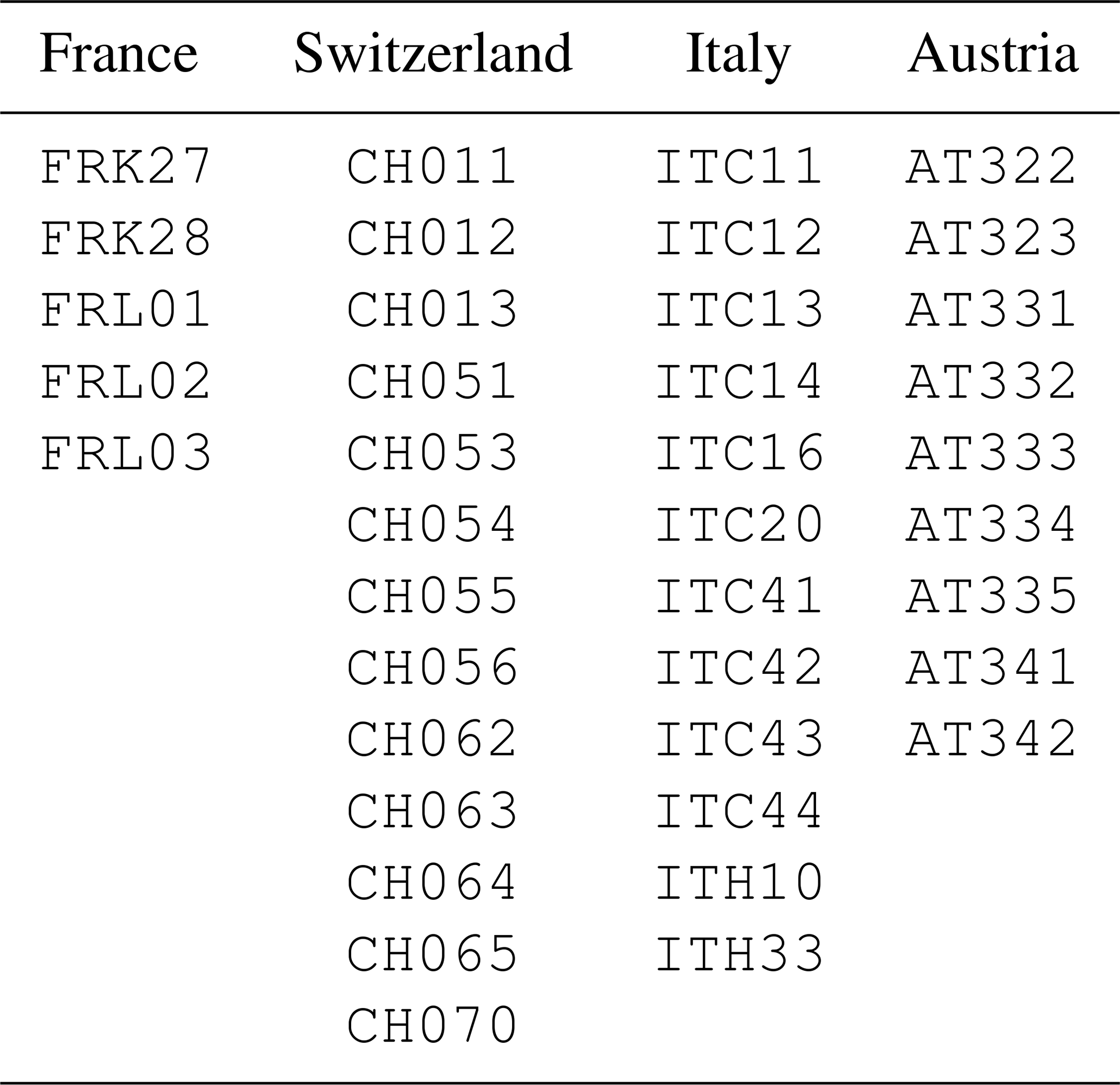
Scripts and data files to recreate our analyses are available for direct download from Figshare (https://doi.org/10.6084/m9.figshare.20552745.v1; Pons and Faranda, 2022).
DF conceived the study within the frame of the ANR project BOREAS, provided expertise on the topic of snowfall modeling in climate studies, and contributed to writing the article. FMEP collected the datasets, reviewed the existing literature, conceived the statistical methodology and the experimental design, wrote the R scripts to analyze the data, and contributed to writing the article.
The contact author has declared that none of the authors has any competing interests.
Publisher's note: Copernicus Publications remains neutral with regard to jurisdictional claims in published maps and institutional affiliations.
The authors thank Saverio Ranciati, for the useful discussion.
This research has been supported by the ANR-TERC (grant no. BOREAS).
This paper was edited by Sarah Perkins-Kirkpatrick and reviewed by two anonymous referees.
Agresti, A.: Foundations of linear and generalized linear models, John Wiley & Sons, ISBN-13 978-1118730034, ISBN-10 1118730038, 2015. a
Atchison, J. and Shen, S. M.: Logistic-normal distributions: Some properties and uses, Biometrika, 67, 261–272, 1980. a
Auer, I., Böhm, R., Jurković, A., Orlik, A., Potzmann, R., Schöner, W., Ungersböck, M., Brunetti, M., Nanni, T., Maugeri, M., Briffa, K., Jones, P., Efthymiadis, D., Mestre, O., Moisselin, J. M., Begert, M., Brazdil, R., Bochnicek, O., Cegnar, T., Gajic-Capka, M., Zaninovic, K., Majstorovic, Z., Szalai, S., Szentimrey, T., and Mercalli, L.: A new instrumental precipitation dataset for the greater alpine region for the period 1800–2002, Int. J. Climatol., 25, 139–166, 2005. a
Auer Jr., A. H.: The rain versus snow threshold temperatures, Weatherwise, 27, 67–67, 1974. a
Ayar, P. V., Vrac, M., Bastin, S., Carreau, J., Déqué, M., and Gallardo, C.: Intercomparison of statistical and dynamical downscaling models under the EURO-and MED-CORDEX initiative framework: present climate evaluations, Clim. Dynam., 46, 1301–1329, 2016. a
Bai, J.: Least squares estimation of a shift in linear processes, J. Time Ser. Anal., 15, 453–472, 1994. a
Bai, J. and Perron, P.: Estimating and testing linear models with multiple structural changes, Econometrica, 47–78, https://doi.org/10.2307/2998540, 1998. a
Bai, J. and Perron, P.: Computation and analysis of multiple structural change models, J. Appl. Econom., 18, 1–22, 2003. a, b
Basu, A., Shioya, H., and Park, C.: Statistical inference: the minimum distance approach, CRC press, https://doi.org/10.1201/b10956, 2011. a
Beaumet, J., Menegoz, M., Gallée, H., Vionnet, V., Fettweis, X., Morin, S., Blanchet, J., Jourdain, N., Wilhelm, B., and Anquetin, S.: Detection of precipitation and snow cover trends in the the European Alps over the last century using model and observational data, in: EGU General Assembly Conference Abstracts, 4–8 May 2020, EGU2020-18274, https://doi.org/10.5194/egusphere-egu2020-18274, 2020. a
Behrangi, A., Yin, X., Rajagopal, S., Stampoulis, D., and Ye, H.: On distinguishing snowfall from rainfall using near-surface atmospheric information: C omparative analysis, uncertainties and hydrologic importance, Q. J. Roy. Meteor. Soc., 144, 89–102, 2018. a
Benjamini, Y. and Hochberg, Y.: Controlling the false discovery rate: a practical and powerful approach to multiple testing, J. R. Stat. Soc. B, 57, 289–300, 1995. a
Bergström, S. and Singh, V.: Computer models of watershed hydrology, The HBV Model, ISBN 9780918334916, 443–476, 1995. a
Bland, J. M. and Altman, D. G.: The odds ratio, Bmj, 320, 1468, https://doi.org/10.1136/bmj.320.7247.1468, 2000. a
Bonelli, P., Lacavalla, M., Marcacci, P., Mariani, G., and Stella, G.: Wet snow hazard for power lines: a forecast and alert system applied in Italy, Nat. Hazards Earth Syst. Sci., 11, 2419–2431, https://doi.org/10.5194/nhess-11-2419-2011, 2011. a
Bonferroni, C.: Teoria statistica delle classi e calcolo delle probabilita, Pubblicazioni del R Istituto Superiore di Scienze Economiche e Commericiali di Firenze, 8, 3–62, https://doi.org/10.1007/978-1-4613-0179-0_88, 1936. a
Copernicus Climate Change Service: ERA5: Fifth generation of ECMWF atmospheric reanalyses of the global climate, https://doi.org/10.24381/cds.adbb2d47, 2017. a, b
Coppola, E., Nogherotto, R., Ciarlo', J. M., Giorgi, F., van Meijgaard, E., Kadygrov, N., Iles, C., Corre, L., Sandstad, M., Somot, S., Nabat, P., Vautard, R., Levavasseur, G., Schwingshackl, C., Sillmann, J., Kjellström, E., Nikulin, G., Aalbers, E., Lenderink, G., Christensen, O. B., Boberg, F., Sørland, S. L., Demory, M., Bülow, K., Teichmann, C., Warrach-Sagi, K., and Wulfmeyer, V.: Assessment of the European climate projections as simulated by the large EURO-CORDEX regional and global climate model ensemble, J. Geophys. Res.-Atmos., 126, e2019JD032356, https://doi.org/10.1029/2019JD032356,, 2021. a
Dai, A.: Temperature and pressure dependence of the rain-snow phase transition over land and ocean, Geophys. Res. Lett., 35, L12802, https://doi.org/10.1029/2008gl033295, 2008. a, b, c, d, e
Darling, D. A.: The kolmogorov-smirnov, cramer-von mises tests, Ann. Math. Stat., 28, 823–838, 1957. a
de Vries, H., Lenderink, G., and van Meijgaard, E.: Future snowfall in western and central Europe projected with a high-resolution regional climate model ensemble, Geophys. Res. Lett., 41, 4294–4299, 2014. a
Ding, B., Yang, K., Qin, J., Wang, L., Chen, Y., and He, X.: The dependence of precipitation types on surface elevation and meteorological conditions and its parameterization, J. Hydrol., 513, 154–163, 2014. a
Ducloux, H. and Nygaard, B. E.: 50-year return-period wet-snow load estimation based on weather station data for overhead line design in France, Nat. Hazards Earth Syst. Sci., 14, 3031–3041, https://doi.org/10.5194/nhess-14-3031-2014, 2014. a
Faranda, D.: An attempt to explain recent changes in European snowfall extremes, Weather Clim. Dynam., 1, 445–458, 2020. a, b, c, d, e, f, g
Fox, J.: Applied regression analysis and generalized linear models, Sage Publications, ISBN-13 978-1452205663, ISBN-10: 1452205663, 2015. a
François, B., Vrac, M., Cannon, A. J., Robin, Y., and Allard, D.: Multivariate bias corrections of climate simulations: which benefits for which losses?, Earth Syst. Dynam., 11, 537–562, https://doi.org/10.5194/esd-11-537-2020, 2020. a
Frei, P., Kotlarski, S., Liniger, M. A., and Schär, C.: Future snowfall in the Alps: projections based on the EURO-CORDEX regional climate models, The Cryosphere, 12, 1–24, https://doi.org/10.5194/tc-12-1-2018, 2018. a
Gay, D. M.: Usage summary for selected optimization routines, Computing science technical report, 153, 1–21, 1990. a
Grouillet, B., Ruelland, D., Vaittinada Ayar, P., and Vrac, M.: Sensitivity analysis of runoff modeling to statistical downscaling models in the western Mediterranean, Hydrol. Earth Syst. Sci., 20, 1031–1047, https://doi.org/10.5194/hess-20-1031-2016, 2016. a
Harder, P. and Pomeroy, J.: Estimating precipitation phase using a psychrometric energy balance method, Hydrol.Process., 27, 1901–1914, 2013. a, b, c, d
Harrell Jr., F. E.: Regression modeling strategies: with applications to linear models, logistic and ordinal regression, and survival analysis, Springer, ISBN 978-3-319-19425-7, 2015. a
Hinde, J.: Logistic Normal Distribution, in: International Encyclopedia of Statistical Science, ISBN 978-3-642-04898-2, 2011. a
Isotta, F. A., Frei, C., Weilguni, V., Perčec Tadić, M., Lassegues, P., Rudolf, B., Pavan, V., Cacciamani, C., Antolini, G., Ratto, S. M., Maraldo, L., Micheletti, S., Bonati, V., Lussana, C., Ronchi, C.,Panettieri, E., Marigo, G., and Vertacnik, G.: The climate of daily precipitation in the Alps: development and analysis of a high-resolution grid dataset from pan-Alpine rain-gauge data, Int. J. Climatol., 34, 1657–1675, 2014. a
Jennings, K. S., Winchell, T. S., Livneh, B., and Molotch, N. P.: Spatial variation of the rain–snow temperature threshold across the Northern Hemisphere, Nat. Commun., 9, 1–9, 2018. a, b, c, d, e, f
Kienzle, S. W.: A new temperature based method to separate rain and snow, Hydrol. Process., 22, 5067–5085, 2008. a, b, c
Kite, G.: The SLURP model, in: Computer models of watershed hydrology, edited by: Singh, V. P., Water Resources Publications, 521–562, 1995. a
Kleiber, C., Hornik, K., Leisch, F., and Zeileis, A.: strucchange: An r package for testing for structural change in linear regression models, J. Stat. Softw., 7, 1–38, 2002. a
Krasting, J. P., Broccoli, A. J., Dixon, K. W., and Lanzante, J. R.: Future changes in Northern Hemisphere snowfall, J. Climate, 26, 7813–7828, 2013. a
Kruskal, W. H. and Wallis, W. A.: Use of ranks in one-criterion variance analysis, J. Am. Stat. Assoc., 47, 583–621, 1952. a, b
Lange, S.: Trend-preserving bias adjustment and statistical downscaling with ISIMIP3BASD (v1.0), Geosci. Model Dev., 12, 3055–3070, https://doi.org/10.5194/gmd-12-3055-2019, 2019. a
L'hôte, Y., Chevallier, P., Coudrain, A., Lejeune, Y., and Etchevers, P.: Relationship between precipitation phase and air temperature: comparison between the Bolivian Andes and the Swiss Alps/Relation entre phase de précipitation et température de l'air: comparaison entre les Andes Boliviennes et les Alpes Suisses, Hydrological Sciences Journal, 50, https://doi.org/10.1623/hysj.2005.50.6.989, 2005. a
Llasat, M. C., Turco, M., Quintana-Seguí, P., and Llasat-Botija, M.: The snow storm of 8 March 2010 in Catalonia (Spain): a paradigmatic wet-snow event with a high societal impact, Nat. Hazards Earth Syst. Sci., 14, 427–441, https://doi.org/10.5194/nhess-14-427-2014, 2014. a
Maraun, D.: Bias correcting climate change simulations-a critical review, Current Climate Change Reports, 2, 211–220, 2016. a
McAfee, S. A., Walsh, J., and Rupp, T. S.: Statistically downscaled projections of snow/rain partitioning for Alaska, Hydrol. Process., 28, 3930–3946, 2014. a
McCabe, G. J. and Wolock, D. M.: Joint variability of global runoff and global sea surface temperatures, J. Hydrometeorol., 9, 816–824, 2008. a
McCabe, G. J. and Wolock, D. M.: Recent declines in western US snowpack in the context of twentieth-century climate variability, Earth Interact., 13, 1–15, 2009. a
Meyer, J., Kohn, I., Stahl, K., Hakala, K., Seibert, J., and Cannon, A. J.: Effects of univariate and multivariate bias correction on hydrological impact projections in alpine catchments, Hydrol. Earth Syst. Sci., 23, 1339–1354, https://doi.org/10.5194/hess-23-1339-2019, 2019. a
Muggeo, V. M.: Estimating regression models with unknown break-points, Stat. Med., 22, 3055–3071, 2003. a, b
Muggeo, V. M.: Segmented: an R package to fit regression models with broken-line relationships, R news, 8, 20–25, 2008. a
Murray, R.: Rain and snow in relation to the 1000–700 mb and 1000–500 mb thicknesses and the freezing level, Meteorol. Mag., 81, 5–8, 1952. a, b
Nikolov, D. and Wichura, B.: Analysis of spatial and temporal distribution of wet snow events in Germany, in: XIII International Workshop on Atmospheric Icing of Structures (IWAIS), IWAIS XIII, Andermatt, Switzerland, 8–11 September 2009, 2009. a
Pan, X., Yang, D., Li, Y., Barr, A., Helgason, W., Hayashi, M., Marsh, P., Pomeroy, J., and Janowicz, R. J.: Bias corrections of precipitation measurements across experimental sites in different ecoclimatic regions of western Canada, The Cryosphere, 10, 2347–2360, https://doi.org/10.5194/tc-10-2347-2016, 2016. a
Pardo, L.: Statistical inference based on divergence measures, CRC press, ISBN 9780429148521, 2018. a
Pipes, A. and Quick, M. C.: UBC watershed model users guide, Department of Civil Engineering, University of British Columbia, 1977. a, b, c, d, e
Pons, F. and Faranda, D.: Statistical reconstruction of European winter snowfall in reanalysis and climate models based on air temperature and total precipitation, figshare [data set], https://doi.org/10.6084/m9.figshare.20552745.v1, 2022. a
Rasmussen, R., Baker, B., Kochendorfer, J., Meyers, T., Landolt, S., Fischer, A. P., Black, J., Thériault, J. M., Kucera, P., Gochis, D., Smith, C., Nitu, R., Hall, M., Ikeda, K., and Gutmann, E.: How well are we measuring snow: The NOAA/FAA/NCAR winter precipitation test bed, B. Am. Meteorol. Soc., 93, 811–829, 2012. a
Scherrer, S. C. and Appenzeller, C.: Swiss Alpine snow pack variability: major patterns and links to local climate and large-scale flow, Clim. Res., 32, 187–199, 2006. a
Schmucki, E., Marty, C., Fierz, C., and Lehning, M.: Simulations of 21st century snow response to climate change in Switzerland from a set of RCMs, Int. J. Climatol., 35, 3262–3273, 2015. a
Smithson, M. and Verkuilen, J.: A better lemon squeezer? Maximum-likelihood regression with beta-distributed dependent variables, Psychologica methods, 11, 54–71, 2006. a, b
Teutschbein, C. and Seibert, J.: Bias correction of regional climate model simulations for hydrological climate-change impact studies: Review and evaluation of different methods, J. Hydrol., 456, 12–29, 2012. a
Teutschbein, C. and Seibert, J.: Is bias correction of regional climate model (RCM) simulations possible for non-stationary conditions?, Hydrol. Earth Syst. Sci., 17, 5061–5077, https://doi.org/10.5194/hess-17-5061-2013, 2013. a, b
US Army Corps of Engineers: Snow hydrology: Summary report of the snow investigations, North Pacific Division Portland, OR, https://doi.org/10.3189/S0022143000024503, 1956. a, b, c
Vautard, R., Kadygrov, N., Iles, C., Boberg, F., Buonomo, E., Bülow, K., Coppola, E., Corre, L., van Meijgaard, E., Nogherotto, R., Sandstad, M., Schwingshakl, C., Somot, S., Aal-bers, E. E., Christensen, O., Ciarlo, J., Demory, M.-E., Giorgi,F., Jacob, D., Jones, R. G., Keuler, K., Kjellström, E., Lenderink,G., Levavasseur, G., Nikulin, G., Sillmann, J., Solidoro, C., Sørland, S., Steger, C., Teichmann, C., Warrach-Sagi, K., and Wulfmeyer, V.: Evaluation of the large EURO-CORDEX regional climate model ensemble, J. Geophys. Res., 125, e2019JD032344, https://doi.org/10.1029/2019JD032344, 2020. a
Vrac, M.: Multivariate bias adjustment of high-dimensional climate simulations: the Rank Resampling for Distributions and Dependences (R2D2) bias correction, Hydrol. Earth Syst. Sci., 22, 3175–3196, https://doi.org/10.5194/hess-22-3175-2018, 2018. a
Vrac, M. and Friederichs, P.: Multivariate-intervariable, spatial, and temporal-bias correction, J. Climate, 28, 218–237, 2015. a
Vrac, M., Drobinski, P., Merlo, A., Herrmann, M., Lavaysse, C., Li, L., and Somot, S.: Dynamical and statistical downscaling of the French Mediterranean climate: uncertainty assessment, Nat. Hazards Earth Syst. Sci., 12, 2769–2784, https://doi.org/10.5194/nhess-12-2769-2012, 2012. a
Vrac, M., Noël, T., and Vautard, R.: Bias correction of precipitation through Singularity Stochastic Removal: Because occurrences matter, J. Geophys. Res.-Atmos., 121, 5237–5258, 2016. a, b
Wen, L., Nagabhatla, N., Lü, S., and Wang, S.-Y.: Impact of rain snow threshold temperature on snow depth simulation in land surface and regional atmospheric models, Adv. Atmos. Sci., 30, 1449–1460, 2013. a, b, c, d
Wilcoxon, F.: Individual comparisons by ranking methods, in: Breakthroughs in statistics, 196–202, Springer, https://doi.org/10.1007/978-1-4612-4380-9_16, 1992. a, b
Wood, S. N.: Generalized additive models: an introduction with R, CRC press, https://doi.org/10.1201/9781315370279, 2017. a
Zeileis, A., Kleiber, C., Krämer, W., and Hornik, K.: Testing and dating of structural changes in practice, Comput. Stat. Data An., 44, 109–123, 2003. a, b
Zubler, E. M., Scherrer, S. C., Croci-Maspoli, M., Liniger, M. A., and Appenzeller, C.: Key climate indices in Switzerland; expected changes in a future climate, Climatic Change, 123, 255–271, 2014. a
- Abstract
- Introduction
- Data
- Methods
- Design of the experiment and statistical method evaluation
- Results
- Discussion
- Conclusions
- Appendix A: Statistical modeling framework
- Code and data availability
- Author contributions
- Competing interests
- Disclaimer
- Acknowledgements
- Financial support
- Review statement
- References