Comparing climate time series – Part 4: Annual cycles

This paper derives a test for deciding whether two time series come from the same stochastic model, where the time series contains periodic and serially correlated components. This test is useful for comparing dynamical model simulations to observations. The framework for deriving this test is the same as in the previous three parts: the time series are first fit to separate autoregressive models, and then the hypothesis that their parameters are equal is tested. This paper generalizes the previous tests to a limited class of nonstationary processes, namely, those represented by an autoregressive model with deterministic forcing terms. The statistic for testing differences in parameters can be decomposed into independent terms that quantify differences in noise variance, differences in autoregression parameters, and differences in forcing parameters (e.g., differences in annual cycle forcing). A hierarchical procedure for testing individual terms and quantifying the overall significance level is derived from standard methods. The test is applied to compare observations of the meridional overturning circulation from the RAPID array to Coupled Model Intercomparison Project Phase 5 (CMIP5) models. Most CMIP5 models are inconsistent with observations, with the strongest differences arising from having too little noise variance, though differences in annual cycle forcing also contribute significantly to discrepancies from observations. This appears to be the first use of a rigorous criterion to decide “equality of annual cycles” in regards to all their attributes (e.g., phases, amplitudes, frequencies) while accounting for serial correlations.

1 Introduction

This is Part 4 of a series of papers on comparing climate time series that are serially correlated. In each of these papers, the basic idea is to fit time series to separate autoregressive (AR) models and then test whether the parameters of the two AR models are equal. A rigorous statistical test was derived for univariate time series (DelSole and Tippett, 2020; Part 1) and multivariate time series (DelSole and Tippett, 2021b; Part 2) and was used as a foundation for diagnosing differences in stochastic processes (DelSole and Tippett, 2022; Part 3). These procedures are equivalent to testing equality of power spectra and equality of autocorrelation functions within the class of functions generated by AR models. The purpose of this work is to generalize these tests to nonstationary processes.

Many climate time series exhibit nonstationary variability, including diurnal cycles, annual cycles, and long-term trends. An established technique for comparing nonstationary variability between models and observations is optimal fingerprinting (Bindoff et al., 2013; Hammerling et al., 2019). This technique is closely related to generalized least squares in which serial correlation of the regression errors is taken into account through a specified covariance matrix. Although most studies focus on long-term trends, fingerprinting could also be applied to other forms of nonstationarity, including diurnal or annual cycles. In many applications, the required covariance matrix is estimated by pooling dynamical model simulations. Unfortunately, such pooling assumes that different dynamical models produce statistically equivalent internal variability, which is dubious (see Parts 1–3 of this paper series). If the covariance matrix is estimated from a single dynamical model, then the sample sizes that can be produced under current computational resources severely limit the dimension of the state space that can be analyzed. The method we propose partly overcomes these limitations.

In the case of annual and diurnal cycles, no standard test exists for deciding whether such cycles are consistent between two data sets. To be sure, some studies test certain aspects of the diurnal or annual cycles. For instance, some studies have shown that the phase and amplitude of the annual cycle of temperature changed over the past half century (Stine et al., 2009; Stine and Huybers, 2012; Cornes et al., 2017; Santer et al., 2018). These results were obtained by isolating one particular feature of the annual cycle that can be computed for each year, say the amplitude or phase of a specified harmonic, and then performing a trend analysis of the resulting time series. Obviously, this strategy depends on carefully choosing the feature on which to focus. For many problems, multiple features of the annual cycle are of interest, and the available methods are not straightforward to generalize to the problem of comparing multiple features of the annual cycle simultaneously. Our goal is to develop such a test.

A standard approach to accounting for seasonality in time series is to filter it out by subtracting last year's value from the present and then modeling the resulting residuals by an ARMA model (Box et al., 2008). An advantage of this approach is that it can adaptively adjust to changes in the phase and amplitude of the annual cycle. A disadvantage is that it removes the annual cycle from the time series and thereby removes the very object of interest. Various other methods for analyzing deterministic signals in the presence of serially correlated noise are reviewed by Chandler and Scott (2011). Some of these methods are heuristic, such as adjusting the degrees of freedom to account for serial correlation. Other methods account for serial correlation at certain steps but fail to propagate the associated uncertainty to the final uncertainty estimates. The method we propose overcomes many of these limitations, although it still contains approximations that will be discussed shortly.

Our starting point is to assume that a climate time series {y_t} can be modeled as

$$\begin{array}{}\text{(1)}& y_t=\sum _{h=\mathrm{1}}^H\left({\stackrel{\mathrm{̃}}{b}}_h\cos \left({\mathit{\omega }}_{h}t\right)+{\stackrel{\mathrm{̃}}{c}}_h\sin \left({\mathit{\omega }}_{h}t\right)\right)+\stackrel{\mathrm{̃}}{\mathit{\mu }}+{\mathit{\eta }}_t,\end{array}$$

where ${\stackrel{\mathrm{̃}}{b}}_h,{\stackrel{\mathrm{̃}}{c}}_h$ are deterministic Fourier coefficients for the annual cycle, H is the total number of annual harmonics, $\stackrel{\mathrm{̃}}{\mathit{\mu }}$ is a deterministic intercept term, and η_t is a serially correlated process. This model is standard in climate studies. We call ${\stackrel{\mathrm{̃}}{b}}_h,{\stackrel{\mathrm{̃}}{c}}_h$ cycle parameters. Since the annual cycle is assumed to be periodic, there is no loss in generality of representing it as a Fourier series. For many climate time series, the annual cycle is well represented using H much less than the Nyquist frequency. For concreteness, let $y_{\mathrm{1}},y_{\mathrm{2}},\mathrm{\dots }$ denote values of the process in consecutive months, in which case the period of the annual cycle is 12 and the Fourier frequencies are ${\mathit{\omega }}_h=\mathrm{2}\mathit{\pi }h/\mathrm{12}$.

The parameters in Eq. (1) could, in principle, be estimated by the method of least squares (or by Fourier transform methods), but this procedure ignores serial correlation in η_t, and hence the resulting confidence intervals would be incorrect. Other methods are reviewed in Chandler and Scott (2011), but most of these are limited in one way or another. For instance, the method of Cochran and Orcutt fails to account for estimation of noise parameters. In contrast, the maximum likelihood method provides a general framework for estimation and inference and yields estimators with attractive properties in the limit of large sample size (e.g., consistency, efficiency). Accordingly, we focus on maximum likelihood estimation (MLE).

If the covariance matrix is known, then MLE leads to generalized least squares (GLS). In practice, however, the covariance matrix of η_t is not known. If stationarity is imposed, then the covariance matrix for η_t has Toeplitz structure, but the number of unknowns still grows with sample size. Unfortunately, this leads to the problem of incidental parameters in which the maximum likelihood estimates are inconsistent even for a large sample size (Neyman and Scott, 1948). The usual approach to obtaining consistent estimates is to impose additional constraints on the covariance matrix in such a way that the number of parameters remains sufficiently small as the sample size grows. A natural constraint is to assume that η_t is a stationary AR process of order p and therefore can be modeled as

$$\begin{array}{}\text{(2)}& {\mathit{\eta }}_t={\mathit{\varphi }}_{\mathrm{1}}{\mathit{\eta }}_{t-\mathrm{1}}+\mathrm{\dots }+{\mathit{\varphi }}_p{\mathit{\eta }}_{t-p}+{\mathit{ϵ}}_t,\end{array}$$

where ${\mathit{\varphi }}_{\mathrm{1}},\mathrm{\dots },{\mathit{\varphi }}_p$ are AR parameters and ϵ_t is Gaussian white noise with zero mean and variance ${\mathit{\sigma }}_{\mathit{ϵ}}^{\mathrm{2}}$, which we denote as

$${\mathit{ϵ}}_t\stackrel{\text{IID}}{\sim }\mathcal{N}(\mathrm{0},{\mathit{\sigma }}_{\mathit{ϵ}}^{\mathrm{2}}).$$

The resulting covariance matrix for η_t has a particular structure that yields an easily computed Cholesky decomposition. An example of this decomposition for an AR(1) model is presented in Chandler and Scott (2011), Sect. 3.3.3, and leads to the Prais–Winsten transformation (see also Davidson and MacKinnon, 2021, Sect. 10.6). More generally, a regression model of the form (1) with noise satisfying the AR(p) model (2) can be re-parameterized into the following AR model with deterministic periodic forcing:

$$\begin{array}{}\text{(3)}& \begin{array}{rl}{y}_t& ={\mathit{\varphi }}_{\mathrm{1}}{y}_{t-\mathrm{1}}+\mathrm{\dots }+{\mathit{\varphi }}_p{y}_{t-p}+\mathit{\mu }\\ & +\sum _{h=\mathrm{1}}^H\left(b_h\cos \left({\mathit{\omega }}_{h}t\right)+c_h\sin \left({\mathit{\omega }}_{h}t\right)\right)+{\mathit{ϵ}}_t.\end{array}\end{array}$$

This kind of re-parameterization is discussed at the end of Sect. 3.3.3 in Chandler and Scott (2011), and here we generalize it and present a detailed procedure for testing hypotheses. An explicit proof of the re-parameterization based on the Cholesky decomposition is complicated by issues related to treatment of the first p values of y_t. In the next section, we bypass these issues by proving that Eqs. (1) and (3) produce stochastically indistinguishable time series, and therefore they necessarily have the same likelihood function. Accordingly, there is no loss of generality in choosing Eqs. (1) or (3) to model the stochastic process. An attractive feature of using Eq. (3) as the fundamental model is that ϵ_t is Gaussian white noise, and therefore the associated likelihood function leads immediately to a linear regression form, for which a large body of results in linear regression theory can be exploited. For this reason, we use Eq. (3) as our fundamental model.

A model of form (3) is called an AR model with exogenous inputs and will be denoted here as ARX(p,H). The specific values of p and H generally are chosen using a model selection criterion such as Akaike's information criterion. The ARX model usually is not derived from first principles, so in any given application its physical interpretation may be unclear. In the end, the persuasiveness of the model depends on how well it captures the statistical properties of the data. The AR model itself has a long track record of success in a huge range of problems, including applications to weather, climate, economics, speech, fisheries, and earthquakes (see Box et al., 2008).

Model (1) would be a natural model framework for applying optimal fingerprinting to comparing annual cycles. However, current applications of fingerprinting do not make the autoregressive assumption (2). The advantage of imposing autoregressive structure for internal variability is that the associated number of parameters is much smaller than the number of parameters required to specify a covariance matrix. Thus, imposing structure on internal variability reduces the number of estimated parameters, leading to more precision. Although a detection and attribution framework could be developed along these lines, we first consider the problem of comparing annual cycles, leaving the comparison of long-term trends to future work. In the end, we derive a framework for testing equality of diurnal or annual cycles that accounts for serially correlated noise.

While our goal is to derive a hypothesis test, our interest is not limited to the mere decision to accept or reject a null hypothesis. After all, we know before looking at any data that the statistical model is too simple to be a complete model of reality. Rather, our goal is to quantify differences in variability between two data sets. Numerous choices exist for measuring differences in variability, but if one is not careful, one might choose a measure with such poor statistical properties as to be useless. For instance, the measure may have a large sampling variance, in which case differences in the measure may be dominated by sampling variability rather than by real differences in the underlying process. This is a real danger for serially correlated processes, as the variance of a statistic tends to increase with the degree of autocorrelation. The virtue of deriving a hypothesis test from a rigorous statistical framework (i.e., the maximum likelihood method) is that it yields a measure with attractive statistical properties, such as having minimum variance in some sense and a well-defined significance test.

Of course, model (3) has some limitations. First, it assumes that annual or diurnal cycles are deterministic functions of time. We believe this assumption is well justified by the fact that the climate system is forced by deterministic periodic cycles in solar insolation. However, this view is not universally accepted, as some studies propose a modulated annual cycle that does not repeat each year (e.g., Wu et al., 2008) or allow Fourier coefficients to be stochastic. Long-term changes in annual cycle could be included by introducing secular terms into the annual cycle forcing. Second, the model assumes that η_t is stationary. For climate time series, it is likely that internal variability changes with season and thus may be cyclostationary. Cyclostationarity may be incorporated into our framework, but this generalization lies beyond the scope of the present paper (in fact, the present work provides a foundation for this generalization). Third, it assumes that internal variability is well modeled by an autoregressive model. Thus, variables like daily precipitation, which is non-Gaussian and intermittent, would not be well captured by a model of form (3). Fourth, large-sample approximations are used to derive sampling distributions, and hence results from small sample sizes should be interpreted cautiously. Finally, the model applies only to scalar time series. The multivariate generalization to vector time series is analogous to the univariate case and follows the transition from Part 1 to Part 2 of this paper series but lies beyond the scope of the present work.

The test derived here ought to be useful for the development of dynamical models. In dynamical model development, limited computational resources mean that only short runs are possible, where annual and diurnal cycles might be the only meaningful differences. In other situations, the observational record is the limiting factor. For instance, sub-annual measurements of the meridional overturning circulation (MOC) have been available only recently (Frajka-Williams et al., 2019). Despite their short span, such observations provide valuable constraints on climate models. The test derived here can be used to decide which version of a climate model is most consistent with observations in both its annual cycle and random variability. We will illustrate this application by applying this test to compare Coupled Model Intercomparison Project Phase 5 (CMIP5) models to observations of MOC from the RAPID array.

2 Justification of the model

We first show that models (1) and (3) yield the same time series when given the same initial conditions and forcing. The proof is considerably simplified by using complex variables, which results in no loss of generality. Specifically, given the sequence $\mathit{\{}{\mathit{ϵ}}_{p+\mathrm{1}},{\mathit{ϵ}}_{p+\mathrm{2}},\mathrm{\dots }\mathit{\}}$ and initial values $\mathit{\{}{y}_{\mathrm{1}},\mathrm{\dots },y_p\mathit{\}}$, the subsequent values $\mathit{\{}{y}_{p+\mathrm{1}},y_{p+\mathrm{2}},\mathrm{\dots }\mathit{\}}$ derived from

$$\begin{array}{}\text{(4)}& y_t={\mathit{\varphi }}_{\mathrm{1}}{y}_{t-\mathrm{1}}+\mathrm{\dots }+{\mathit{\varphi }}_p{y}_{t-p}+\sum _{h=\mathrm{0}}^H{d}_h{e}^{it{\mathit{\omega }}_h}+{\mathit{ϵ}}_t\end{array}$$

are the same as those derived from

$$\begin{array}{}\text{(5)}& y_t=\sum _{h=\mathrm{0}}^H{\stackrel{\mathrm{̃}}{d}}_h{e}^{it{\mathit{\omega }}_h}+{\mathit{\eta }}_t,\end{array}$$

where η_t is defined in Eq. (2) and

$$\begin{array}{}\text{(6)}& {\displaystyle }{d}_h{\displaystyle }={\stackrel{\mathrm{̃}}{d}}_h\left(\mathrm{1}-{\mathit{\varphi }}_{\mathrm{1}}{e}^{-i{\mathit{\omega }}_h}-\mathrm{\dots }-{\mathit{\varphi }}_p{e}^{-i{\mathit{\omega }}_{h}p}\right).\end{array}$$

Note that Eqs. (1) and (3) are merely the real parts of Eqs. (5) and (4) under the identifications ${\stackrel{\mathrm{̃}}{d}}_h={\stackrel{\mathrm{̃}}{b}}_h-i{\stackrel{\mathrm{̃}}{c}}_h$ and $d_h=b_h-i{c}_h$, respectively. To prove the above assertion, substitute Eq. (5) into Eq. (4) and then note that the time-periodic terms cancel due to Eq. (6), leaving Eq. (2). The first p values of η_t are obtained from the first p residuals from Eq. (5). Note that the intercept terms are incorporated into the above model formulations by defining d₀=μ and ${\stackrel{\mathrm{̃}}{d}}_{\mathrm{0}}=\stackrel{\mathrm{̃}}{\mathit{\mu }}$.

Incidentally, it is also possible to prove that all solutions of Eq. (4) can be written in the form of Eq. (5), but the proof requires more steps and is not required for our purposes. The proof is to recognize that Eq. (4) is a linear, finite-difference equation, and therefore the general solution can be obtained by solving for homogeneous and particular solutions separately and adding them together. The end result is that the periodic term in Eq. (5) is the particular solution to Eq. (4) to periodic forcing, and η_t in Eq. (5) is the sum of the homogeneous solution and the particular solution of Eq. (4) to ϵ_t.

Thus, Eqs. (4) and (5) represent exactly the same stochastic process, under suitable identification of the parameters. Equivalently, we say that Eq. (4) is a re-parameterization of (5), or vice versa. The two models differ by whether the cycle parameters d_h or ${\stackrel{\mathrm{̃}}{d}}_h$ are used to parameterize the cycle. It can be shown that the periodic part of Eq. (5) is the asymptotic response of Eq. (4) in the absence of noise (i.e., ϵ_t=0). Thus, the parameter d_h is identified with periodic forcing, and ${\stackrel{\mathrm{̃}}{d}}_h$ is identified with periodic response. As indicated in Eq. (6), the response ${\stackrel{\mathrm{̃}}{d}}_h$ is a nonlinear function of the forcing parameter d_h and AR parameters $\mathit{\{}{\mathit{\varphi }}_{\mathrm{1}},\mathrm{\dots },{\mathit{\varphi }}_p\mathit{\}}$. This fact is illustrated in Fig. 1, which shows the long-term response of a noise-free version of Eq. (4) for different values of ϕ₁.

If we detect a difference in parameters, we do not know whether the difference is dominated by a difference in AR parameters or in cycle parameters. To isolate the source, tests on subcomponents of the model need to be performed. At this step, a difference arises between testing equality of d_h in Eq. (4) and testing equality of ${\stackrel{\mathrm{̃}}{d}}_h$ in Eq. (5). In general, equality of d_h does not imply equality of ${\stackrel{\mathrm{̃}}{d}}_h$, or vice versa. However, if the AR parameters are equal, then it follows from Eq. (6) that equality of d_h is equivalent to equality of ${\stackrel{\mathrm{̃}}{d}}_h$, and our decision about equality of d_h will agree with our decision about equality of ${\stackrel{\mathrm{̃}}{d}}_h$. This is attractive because there is no compelling reason to favor testing equality of d_h over ${\stackrel{\mathrm{̃}}{d}}_h$. By testing equality of AR parameters before equality of d_h or ${\stackrel{\mathrm{̃}}{d}}_h$, our decision about equality of d_h will be consistent with our decision about equality of ${\stackrel{\mathrm{̃}}{d}}_h$. This fact motivates testing equality of AR parameters prior to testing equality of cycle parameters (either d_h or ${\stackrel{\mathrm{̃}}{d}}_h$).

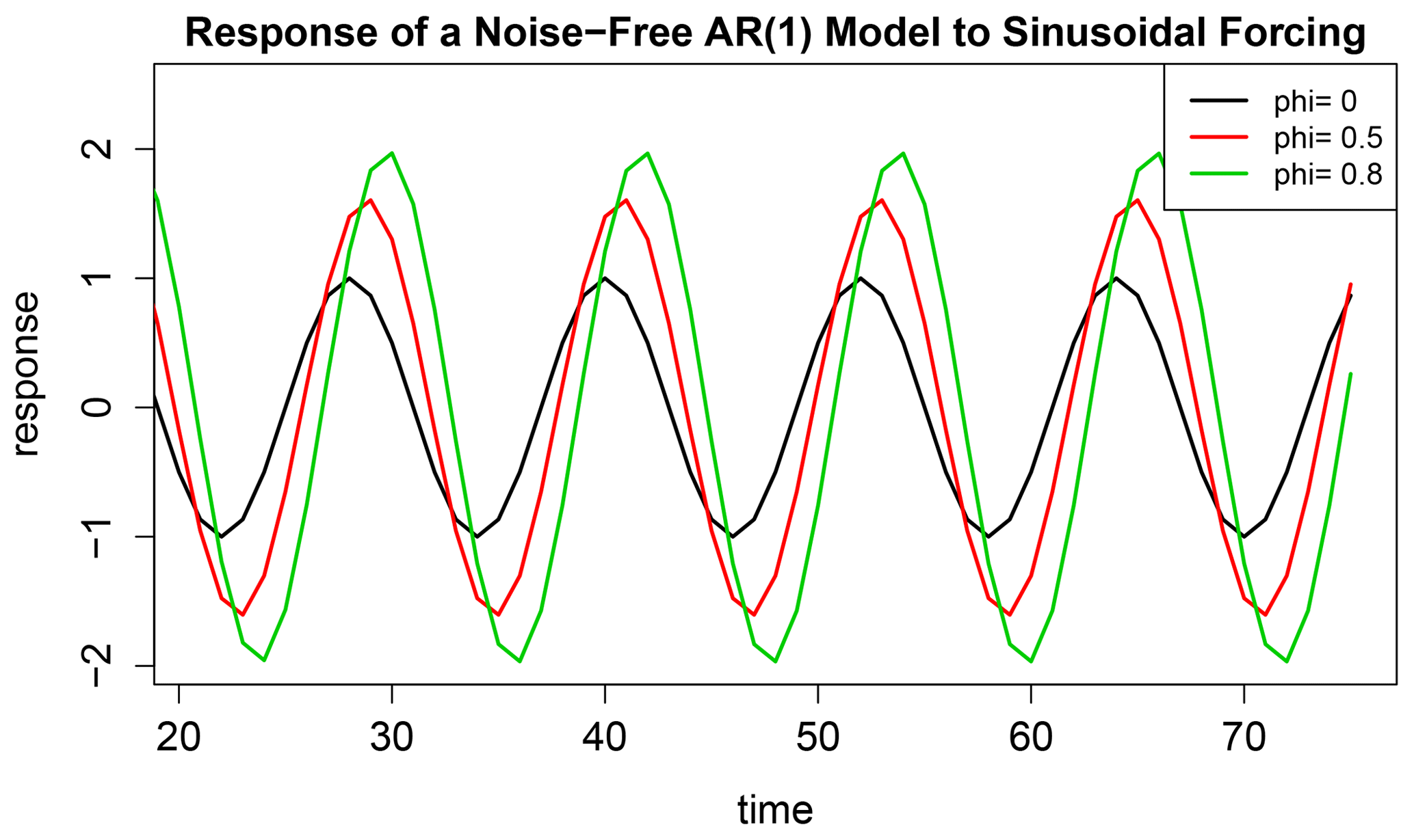
Figure 1 The periodic response of a noise-free AR(1) model to sinusoidal forcing for AR parameters ϕ=0, 0.5, and 0.8. The forcing is shown by the black curve, which is equivalent to the response for ϕ=0.

3 General procedure

The standard method for estimating ARX models is the maximum likelihood method (Brockwell and Davis, 1991; Box et al., 2008). Unfortunately, the resulting estimates have complicated distributions even in the Gaussian case (Brockwell and Davis, 1991, chap. 6). Nevertheless, for asymptotically large sample sizes, the distributions of the parameter estimates are consistent with those derived from linear regression theory; e.g., see theorem 8.1.2 and Sect. 8.9 of Brockwell and Davis (1991) and Appendix A7.5 of Box et al. (2008). Accordingly, we first describe an exact test for equality of parameters for regression models and then invoke asymptotic theory to apply that test to equality of ARX models.

Tests for equality of regression parameters have appeared previously (Fisher, 1970; Rao, 1973). However, merely detecting a difference in models would be unsatisfying because this result gives no information about which components of the regression model dominate the differences. Accordingly, we test hypotheses about particular components of the model through a sequence of nested tests while accounting for multiple-testing issues. The procedure presented here is an adaptation of the sequential test derived by Hogg (1961) and Seber (2015). We give a brief description of the test here and provide more mathematical details in Appendix B. Relative to the test derived in Part 2 (DelSole and Tippett, 2021b), the test derived here is more general in that it tests equality of an arbitrary subset of regression coefficients.

The general problem is to compare models of the form

$$\begin{array}{}\text{(7)}& {\displaystyle }\mathit{y}& {\displaystyle }=\mathit{j}\mathit{\mu }+{\mathit{X}}_{\mathrm{2}}{\mathit{\beta }}_{\mathrm{2}}+{\mathit{X}}_{\mathrm{3}}{\mathit{\beta }}_{\mathrm{3}}+\mathit{ϵ}\text{ and }\mathit{ϵ}\sim \mathcal{N}(\mathbf{0},{\mathit{\sigma }}^{\mathrm{2}}\mathbf{I}),\text{(8)}& {\displaystyle }{\mathit{y}}^{*}& {\displaystyle }={\mathit{j}}^{*}{\mathit{\mu }}^{*}+{\mathit{X}}_{\mathrm{2}}^{*}{\mathit{\beta }}_{\mathrm{2}}^{*}+{\mathit{X}}_{\mathrm{3}}^{*}{\mathit{\beta }}_{\mathrm{3}}^{*}+{\mathit{ϵ}}^{*}\text{ and }{\mathit{ϵ}}^{*}\sim \mathcal{N}(\mathbf{0},{\mathit{\sigma }}^{*\mathrm{2}}\mathbf{I}),\end{array}$$

where j and j^* are a vector of ones to account for the intercept, ϵ and ϵ^* are independent, and the other terms have dimensions

$$\begin{array}{c}{\displaystyle }\mathit{y}\in {\mathbb{R}}^N,{\mathit{X}}_k\in {\mathbb{R}}^{N\times K_k},{\mathit{\beta }}_k\in {\mathbb{R}}^{K_k},\mathit{j}\in {\mathbb{R}}^N,\\ {\displaystyle }{\mathit{y}}^{*}\in {\mathbb{R}}^{N^{*}},{\mathit{X}}_k^{*}\in {\mathbb{R}}^{N^{*}\times K_k},{\mathit{\beta }}_k^{*}\in {\mathbb{R}}^{K_k},{\mathit{j}}^{*}\in {\mathbb{R}}^{N^{*}},\end{array}$$

where $k=\mathrm{2},\mathrm{3}$.

Model (3) can be written in this form, as shown explicitly in Appendix A. If a model difference is detected, the next natural question is whether this difference is dominated by a difference in noise variance, AR parameters, or cycle parameters. The order in which we test these components is an important issue. To appreciate this, it is instructive to recall the difference-in-means test. The standard difference-in-means test is the Student's t test, which examines equality of means assuming the variances are equal. However, if the variances are unequal, the Student's t test is not appropriate because the distribution of the t statistic depends on the ratio of variances. This is the central issue in the Behrens–Fisher problem. Our procedure would reduce to the t test if we tested equality of μ in Eq. (3) under vanishing AR parameters and Fourier coefficients. Consequently, we can anticipate that when testing equality of regression coefficients, the sampling distribution of the test statistic will also depend on the ratio of variances. To avoid this situation, tests for equality of regression coefficients should assume equality of noise variances. That is, even if our goal is to compare only annual cycles, a usable test requires checking for equality of variances. This requirement is analogous to having to check for equality of variances before using the Student's t test.

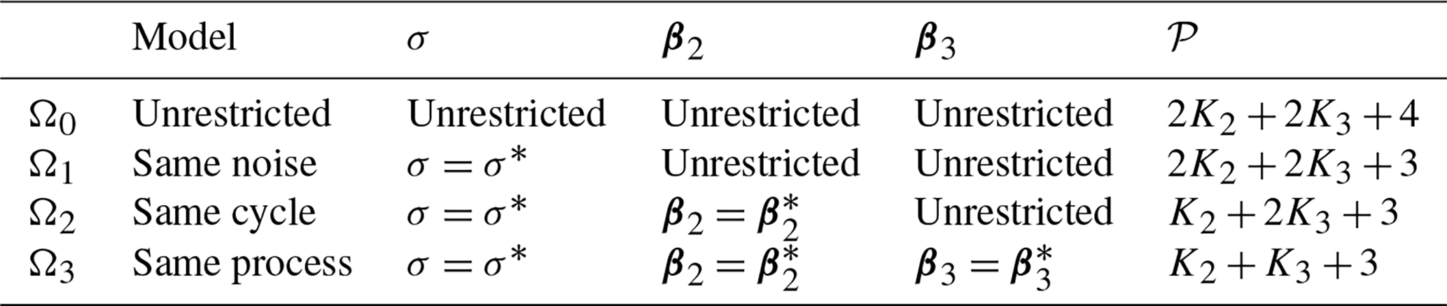
For reasons discussed in Sect. 2, we test equality of AR parameters before testing equality of cycle parameters. These considerations dictate the hierarchy of hypotheses given in Table 1. Under this hierarchy, the vector β₂ contains the AR parameters $\mathit{\{}{\mathit{\varphi }}_{\mathrm{1}},\mathrm{\dots },{\mathit{\varphi }}_p\mathit{\}}$, and the vector β₃ contains the annual cycle parameters {b_h,c_h}. Thus, K₂=p and K₃=2H. In climate studies, it is customary to ignore biases, and therefore no restriction is imposed on μ and μ^* in the hypotheses in Table 1 (although the hypothesis $\mathit{\mu }={\mathit{\mu }}^{*}$ could easily be included in the hierarchy if desired).

Note that Ω₀ denotes the least restrictive hypothesis and does not denote the null hypothesis. This notation is adopted so that the order of the tests in the hierarchy conveniently starts with Ω₀ and then proceeds to ${\mathrm{\Omega }}_{\mathrm{1}},{\mathrm{\Omega }}_{\mathrm{2}},{\mathrm{\Omega }}_{\mathrm{3}}$. Also, additional hypotheses ${\mathrm{\Omega }}_{\mathrm{4}},{\mathrm{\Omega }}_{\mathrm{5}},\mathrm{\dots }$ may be added simply by adding rows to the bottom of Table 1. The procedure described here and in Appendix B can be generalized to an arbitrary number of hypotheses.

Table 1 Table summarizing the hypotheses considered in the hierarchical test procedure. 𝒫 in the last column denotes the number of parameters estimated.

The maximized likelihoods for hypotheses ${\mathrm{\Omega }}_{\mathrm{0}},{\mathrm{\Omega }}_{\mathrm{1}},{\mathrm{\Omega }}_{\mathrm{2}},{\mathrm{\Omega }}_{\mathrm{3}}$ are, respectively,

$$\begin{array}{}\text{(9)}& {\displaystyle }{L}_{{\mathrm{\Omega }}_{\mathrm{0}}}& {\displaystyle }=\left(\mathrm{2}\mathit{\pi }e{\stackrel{\mathrm{‾}}{\mathit{\sigma }}}^{\mathrm{2}}{)}^{-N/\mathrm{2}}\right(\mathrm{2}\mathit{\pi }e{\stackrel{\mathrm{‾}}{\mathit{\sigma }}}^{*\mathrm{2}}{)}^{-N^{*}/\mathrm{2}},\text{(10)}& {\displaystyle }{L}_{{\mathrm{\Omega }}_{\mathrm{1}}}& {\displaystyle }=(\mathrm{2}\mathit{\pi }e{\stackrel{\mathrm{‾}}{\mathit{\sigma }}}_{{\mathrm{\Omega }}_{\mathrm{1}}}^{\mathrm{2}}{)}^{-(N+N^{*})/\mathrm{2}},\text{(11)}& {\displaystyle }{L}_{{\mathrm{\Omega }}_{\mathrm{2}}}& {\displaystyle }=(\mathrm{2}\mathit{\pi }e{\stackrel{\mathrm{‾}}{\mathit{\sigma }}}_{{\mathrm{\Omega }}_{\mathrm{2}}}^{\mathrm{2}}{)}^{-(N+N^{*})/\mathrm{2}},\text{(12)}& {\displaystyle }{L}_{{\mathrm{\Omega }}_{\mathrm{3}}}& {\displaystyle }=(\mathrm{2}\mathit{\pi }e{\stackrel{\mathrm{‾}}{\mathit{\sigma }}}_{{\mathrm{\Omega }}_{\mathrm{3}}}^{\mathrm{2}}{)}^{-(N+N^{*})/\mathrm{2}},\end{array}$$

where ${\stackrel{\mathrm{‾}}{\mathit{\sigma }}}^{*\mathrm{2}},{\stackrel{\mathrm{‾}}{\mathit{\sigma }}}^{\mathrm{2}},{\stackrel{\mathrm{‾}}{\mathit{\sigma }}}_{{\mathrm{\Omega }}_{\mathrm{1}}}^{\mathrm{2}},{\stackrel{\mathrm{‾}}{\mathit{\sigma }}}_{{\mathrm{\Omega }}_{\mathrm{2}}}^{\mathrm{2}},{\stackrel{\mathrm{‾}}{\mathit{\sigma }}}_{{\mathrm{\Omega }}_{\mathrm{3}}}^{\mathrm{2}}$ are defined in Appendix B. The statistic for testing Ω_i+k against Ω_i is called the deviance (Hastie et al., 2009, p. 221) and defined as

$$D_{{\mathrm{\Omega }}_{i:i+k}}=-\mathrm{2}\log L_{{\mathrm{\Omega }}_{i+k}}+\mathrm{2}\log L_{{\mathrm{\Omega }}_i}.$$

The deviance vanishes when the likelihoods are equal. Because $L_{{\mathrm{\Omega }}_{\mathrm{3}}}\le L_{{\mathrm{\Omega }}_{\mathrm{2}}}\le L_{{\mathrm{\Omega }}_{\mathrm{1}}}\le L_{{\mathrm{\Omega }}_{\mathrm{0}}}$, the deviance is positive when the likelihoods differ. Thus, the deviance effectively measures the “distance” between likelihoods, with larger values indicating stronger differences between likelihoods. If Ω_i+k is true, then $D_{{\mathrm{\Omega }}_{i:i+k}}$ has the asymptotic distribution

$$\begin{array}{}\text{(13)}& D_{{\mathrm{\Omega }}_{i:i+k}}\sim {\mathit{\chi }}_{{\mathcal{P}}_i-{\mathcal{P}}_{i+k}}^{\mathrm{2}},\end{array}$$

where 𝒫_i is the number of estimated parameters under Ω_i indicated in Table 1. Large values of $D_{{\mathrm{\Omega }}_{i:i+k}}$ indicate rejecting Ω_i+k. In effect, $D_{{\mathrm{\Omega }}_{i:i+k}}$ measures the difference between models Ω_i and Ω_i+k.

The tests associated with $D_{{\mathrm{\Omega }}_{\mathrm{1}:\mathrm{2}}}$ and $D_{{\mathrm{\Omega }}_{\mathrm{2}:\mathrm{3}}}$ are standard analysis of variance tests. For instance, in R, the tests are performed with the commands anova(Model2, Model1) and anova(Model3, Model2), respectively, where Model1, Model2, Model3 are the model fits from lm under Ω₁,Ω₂, and Ω₃, respectively. However, the equality of noise test associated with $D_{{\mathrm{\Omega }}_{\mathrm{0}:\mathrm{1}}}$ is not part of a standard analysis of variance decomposition. In fact, analysis of variance assumes variables come from populations with the same variance. Thus, the tests proposed here include more than a standard variance decomposition: rather, they constitute a deviance decomposition. This fact and other shortcomings of the standard analysis of variance decomposition are discussed in more detail in Appendix B.

The deviances satisfy the identity

$$\begin{array}{}\text{(14)}& D_{{\mathrm{\Omega }}_{\mathrm{0}:\mathrm{3}}}=D_{{\mathrm{\Omega }}_{\mathrm{0}:\mathrm{1}}}+D_{{\mathrm{\Omega }}_{\mathrm{1}:\mathrm{2}}}+D_{{\mathrm{\Omega }}_{\mathrm{2}:\mathrm{3}}},\end{array}$$

which allows us to quantify how differences in particular aspects of the ARX model contribute to the total deviance. We use the following terminology.

$$\begin{array}{ll}{\displaystyle }{D}_{{\mathrm{\Omega }}_{\mathrm{0}:\mathrm{3}}}& {\displaystyle }\text{ total deviance}\\ {\displaystyle }{D}_{{\mathrm{\Omega }}_{\mathrm{0}:\mathrm{1}}}& {\displaystyle }\text{ noise deviance}\\ {\displaystyle }{D}_{{\mathrm{\Omega }}_{\mathrm{1}:\mathrm{2}}}& {\displaystyle }\text{ AR deviance}\\ {\displaystyle }{D}_{{\mathrm{\Omega }}_{\mathrm{2}:\mathrm{3}}}& {\displaystyle }\text{ cycle deviance}\end{array}$$

Since multiple hypotheses arise, the problem of multiple testing needs to be addressed. Appendix B shows that the components in Eq. (14) are mutually stochastically independent when Ω₃ is true. This independence follows from the fact that the hypotheses are nested such that ${\mathrm{\Omega }}_{\mathrm{3}}\subseteq {\mathrm{\Omega }}_{\mathrm{2}}\subseteq {\mathrm{\Omega }}_{\mathrm{1}}\subseteq {\mathrm{\Omega }}_{\mathrm{0}}$, and the estimates satisfy the appropriate properties of sufficiency and completeness required for such independence (see Sect. 7.9 of Hogg et al., 2019). This independence is proven in a more elementary way in Appendix B. The independence of deviances also allows quantification of the family-wise error rate (FWER) of the multiple tests. For testing Ω₃ against Ω₀, a FWER of 5 % can be achieved by setting the type-I error rate of each test to be

$$\mathrm{1}-(\mathrm{1}-\mathrm{0.05}{)}^{\mathrm{1}/\mathrm{3}}\approx \mathrm{1.7}\mathit{\%}.$$

See Appendix B for further details.

Because the hypotheses are nested and $D_{{\mathrm{\Omega }}_{\mathrm{0}:\mathrm{1}}},D_{{\mathrm{\Omega }}_{\mathrm{1}:\mathrm{2}}},D_{{\mathrm{\Omega }}_{\mathrm{2}:\mathrm{3}}}$ are independent, there exists a natural stepwise testing procedure. This procedure is discussed in Hogg (1961), from which the following is based. First, $D_{{\mathrm{\Omega }}_{\mathrm{0}:\mathrm{1}}}$ is tested for significance based on Eq. (13). If it is significantly large, then we decide that Ω₁ is false and stop testing. On the other hand, if $D_{{\mathrm{\Omega }}_{\mathrm{0}:\mathrm{1}}}$ is not significant, then $D_{{\mathrm{\Omega }}_{\mathrm{1}:\mathrm{2}}}$ is tested for significance. If it is significant, then we decide that Ω₁ is true but Ω₂ is false and stop testing. On the other hand, if $D_{{\mathrm{\Omega }}_{\mathrm{1}:\mathrm{2}}}$ is not significant, then $D_{{\mathrm{\Omega }}_{\mathrm{2}:\mathrm{3}}}$ is tested for significance. If it is significant, then we conclude that Ω₂ is true but Ω₃ is false. If $D_{{\mathrm{\Omega }}_{\mathrm{2}:\mathrm{3}}}$ is not significant, then we conclude that no significant difference in ARX models is detected.

4 Diagnostics

Once a significant difference in a component of the ARX model is identified, there still remains the question of precisely how that component differs between ARX models. In Appendix B, we show that the noise deviance $D_{{\mathrm{\Omega }}_{\mathrm{0}:\mathrm{1}}}$ can be written as a function of the variance ratio

$$F^{*}={\displaystyle \frac{{\stackrel{\mathrm{‾}}{\mathit{\sigma }}}^{\mathrm{2}}}{{\stackrel{\mathrm{‾}}{\mathit{\sigma }}}^{*\mathrm{2}}}}.$$

As a result, the test for Ω₁ is equivalent to testing differences in variance based on the F test. Importantly, the F test is applied not to the original time series, but to residuals of the ARX models. This is important because the original time series may be serially correlated and thereby not satisfy the assumptions of the F test. In contrast, the residuals from an ARX model tend to be closer to white noise and thereby better satisfy the assumptions of the F test.

Although we have explored various diagnostics for optimally decomposing AR deviances and cycle deviances, we found it much more instructive to simply plot the corresponding autocorrelation function or the annual cycle response of the ARX model, and indicate the ones that differ significantly from that derived from observations. The autocorrelation of an AR(p) model can be derived by standard methods (e.g., see Box et al., 2008, Sect. 3.2.2).

5 Model selection

To apply our procedure, the order of the AR process and the number of harmonics to include in the model must be specified. These must be the same in the two models being compared; otherwise, we know the processes differ and there is no need to perform the test. Whatever criterion is used, it inevitably chooses different orders and a different number of harmonics for different data sets. In such cases, we choose the highest order and the largest number of harmonics among the results. Our rationale is that underfitting is more serious than overfitting because underfitting leads to residuals with serial correlations that invalidate the distributional assumptions. In contrast, overfitting is taken into account by the test because the test makes no assumption about the value of the regression coefficients, and therefore it includes the case of overfitting in which some coefficients vanish. The main detrimental effect of overfitting is to reduce statistical power: i.e., for a given difference in ARX models, the difference becomes harder to detect as the degree of overfitting increases. This loss of power is not a serious concern in this study because, for our data, differences grow rapidly with the number of predictors.

We choose the order and number of harmonics using a criterion based on a corrected version of Akaike's information criterion (see DelSole and Tippett, 2021a). Strictly speaking, the ARX model contains a mixture of random and deterministic components and this fact should be taken into account in the criterion. The generalization of Akaike's information criterion to the case of a mixture of random and deterministic predictors has been derived in DelSole and Tippett (2021a) and is called AICm (“m” stands for mixture). The explicit equation for this criterion is given in Appendix B (e.g., see Eq. B2).

6 Data

We analyze the net transport of the Atlantic meridional overturning circulation (AMOC) at 26^∘ N. This choice was motivated by the availability of monthly estimates from the RAPID array (Frajka-Williams et al., 2019). At present, this time series is of length 190 months and lies within the 17-year period 2004–2020. This observational period is relatively short, and hence the associated forced variability, such as by aerosols or greenhouse gases, is small relative to internal variability and assumed to be negligible. For climate simulations, we use preindustrial control simulations from CMIP5 (Taylor et al., 2012). Control simulations use forcings that have only diurnal and annual cycles and contain no forced variability on interannual timescales. To avoid climate drift, a second-order polynomial in time is removed from the last 500 years of each control simulation (this has no impact on the results because the quadratic polynomial over the 500-year period is virtually constant over 17 years). The model variable is the maximum MOC streamfunction at 26^∘ N. Ten CMIP5 models have this variable available.

The first observation from RAPID occurs in April. We sample a 190-month sequence (called the “first half”) from each CMIP5 control simulation starting from the first April in the last 500 years of simulation. Then, the subsequent 190-month sequence (called the “second half”) is used as an independent sample. Note that the second sample does not begin in May because 190 is not divisible by 12. This difference in phase τ is taken into account when specifying the annual cycle forcing for the two ARX models (i.e., by specifying τ=5 and τ=195 in Eq. (A1) for X₂ and ${\mathit{X}}_{\mathrm{2}}^{*}$, respectively).

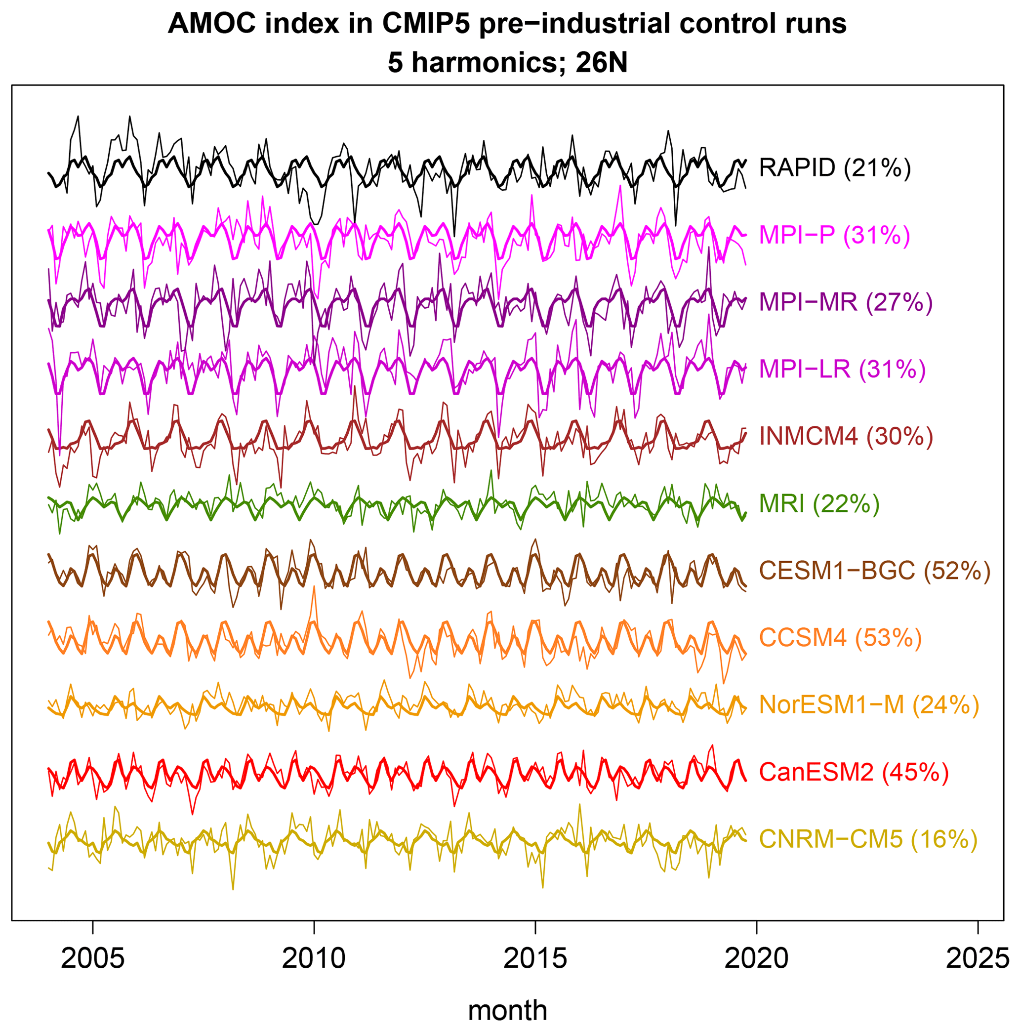
Figure 2 Monthly time series of the maximum transport at 26^∘ N (thin curves) from observations (RAPID; top, black curve) and CMIP5 models (colored curves, with model names at the right end). The thick curves show the best-fit annual cycle based on five annual harmonics. The percentages next to the names are the percent variance explained by the annual cycle (i.e., the R² of the annual cycle). The annual cycle is computed by ordinary least squares without accounting for serial correlation. The time series have been offset relative to each other by an additive constant.

7 Results

The time series under investigation are shown in Fig. 2. One can see a variety of similarities and differences between observational and dynamical model time series. Based on visual comparisons, one might suggest that NorESM1-M differs the most from observations due to its much smaller amplitude, while the MPI models are most similar to observations. However, these are subjective impressions. The purpose of this paper is to decide objectively which of the simulated time series are most statistically similar to observations. Moreover, for the models that differ, we want to rank CMIP5 models in order of dissimilarity to observations and diagnose the nature of the dissimilarities.

As discussed earlier, the order of the AR model and the number of annual harmonics are selected by minimizing a criterion called AICm (DelSole and Tippett, 2021a). For consistency, we restrict simulation time series to be of the same length as that of observations. A representative example of AICm for varying p and H is shown in Fig. 3. In this case, the minimum AICm occurs for a third-order AR process with three annual harmonics. Repeating this procedure for each CMIP5 model reveals at least two cases in which five annual harmonics are chosen (not shown), which is nearly the Nyquist frequency. Accordingly, following the discussion in Sect. 5, we choose H=5 annual harmonics for all cases. After fixing H=5, we use AICm to select p. The resulting AICm is shown in Fig. 4. The maximum selected order is 3, hence we choose p=3 and H=5 for all ARX models.

If the ARX(3,5) model is adequate, then the residuals should resemble Gaussian white noise. To check this, we show the autocorrelation function of the residuals of the ARX(3,5) models in Fig. 5. As can be seen, the residuals have insignificant autocorrelations, except for two isolated cases which are marginal and not significant given the multiple comparisons.

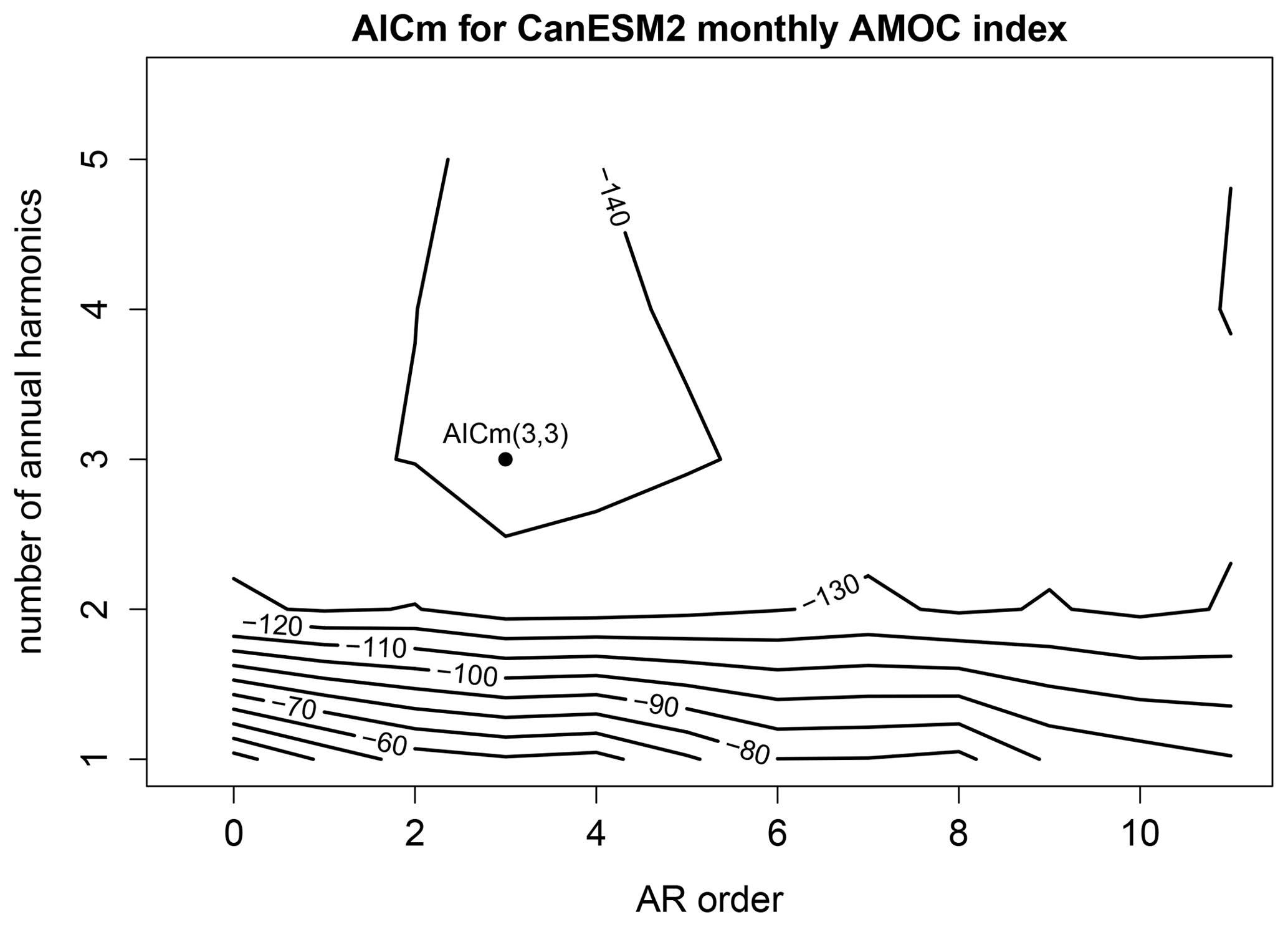
Figure 3 The AICm for fitting time series from the CanEMS2 model to ARX models of the form (3), as a function of the order of the AR process p (x axis) and the number of annual harmonics H (y axis). The ARX model with the smallest AICm is indicated by a dot and is labeled.

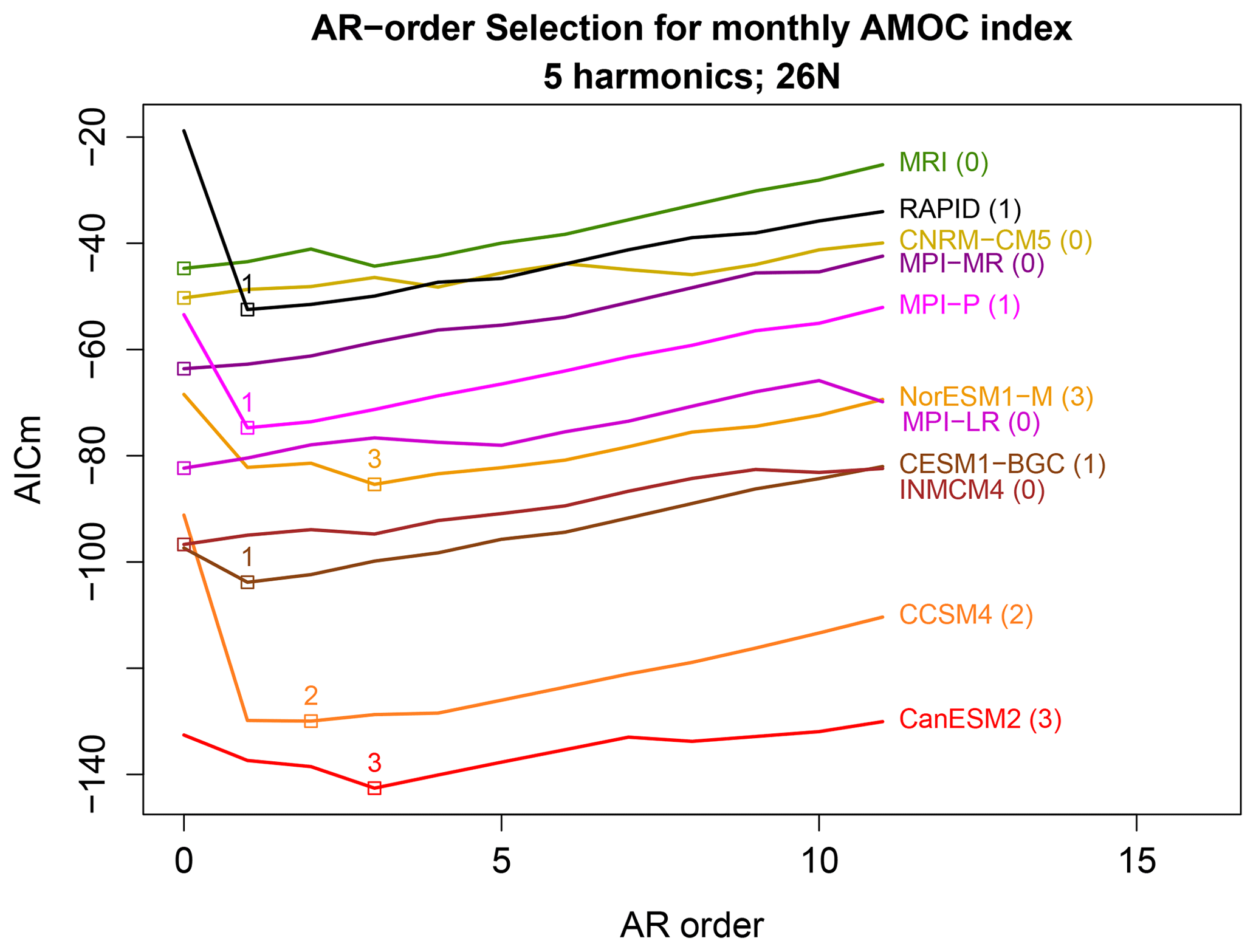
Figure 4 The AICm for fitting time series from each CMIP5 model to ARX models of the form (3), as a function of the order of the AR process p and for the number of annual harmonics H=5. The minimum AICm for each CMIP5 is indicated by a square, and the associated order is indicated above the square (provided it is greater than zero). AICm has not been offset for each model – the different levels of AICm reflect differences in time series.

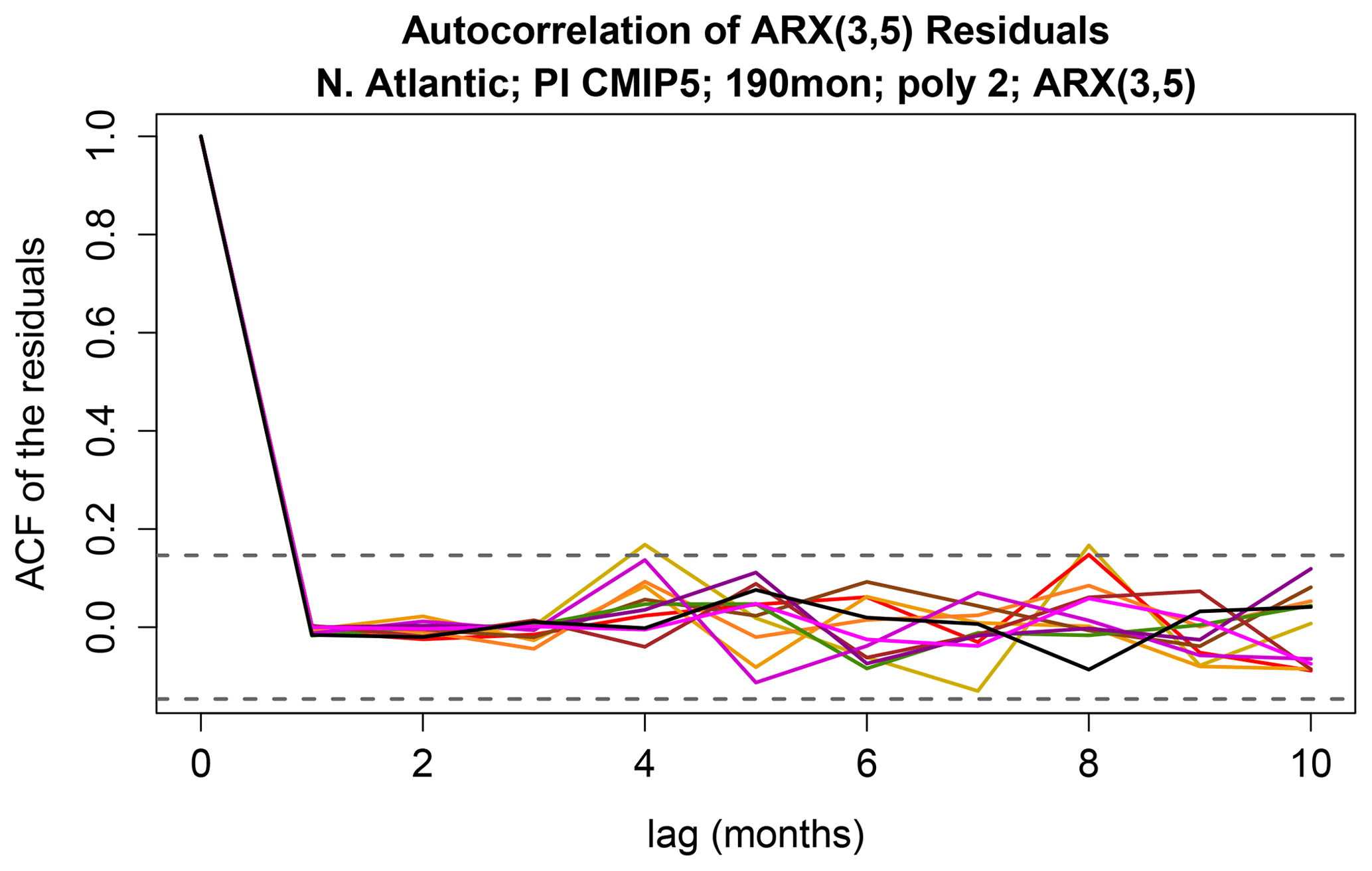
Figure 5 The autocorrelation function of the residuals of the ARX models. The horizontal dashed lines show the upper and lower 5 % confidence limits for zero correlation.

Having chosen the ARX(3,5) model, we next fit time series from observations and from a CMIP5 model and evaluate the total deviance $D_{{\mathrm{\Omega }}_{\mathrm{0}:\mathrm{3}}}$, which is used to test the hypothesis Ω₃ that all parameters in the respective ARX(3,5) models are equal. The results, shown in Fig. 6, reveal that the deviances for the MPI models fall below the significance threshold, indicating that the MPI models are statistically indistinguishable from observations. The other models exceed the significance threshold and therefore differ from observations. As anticipated from Fig. 2, the deviance for the NorESM1-M model is relatively high.

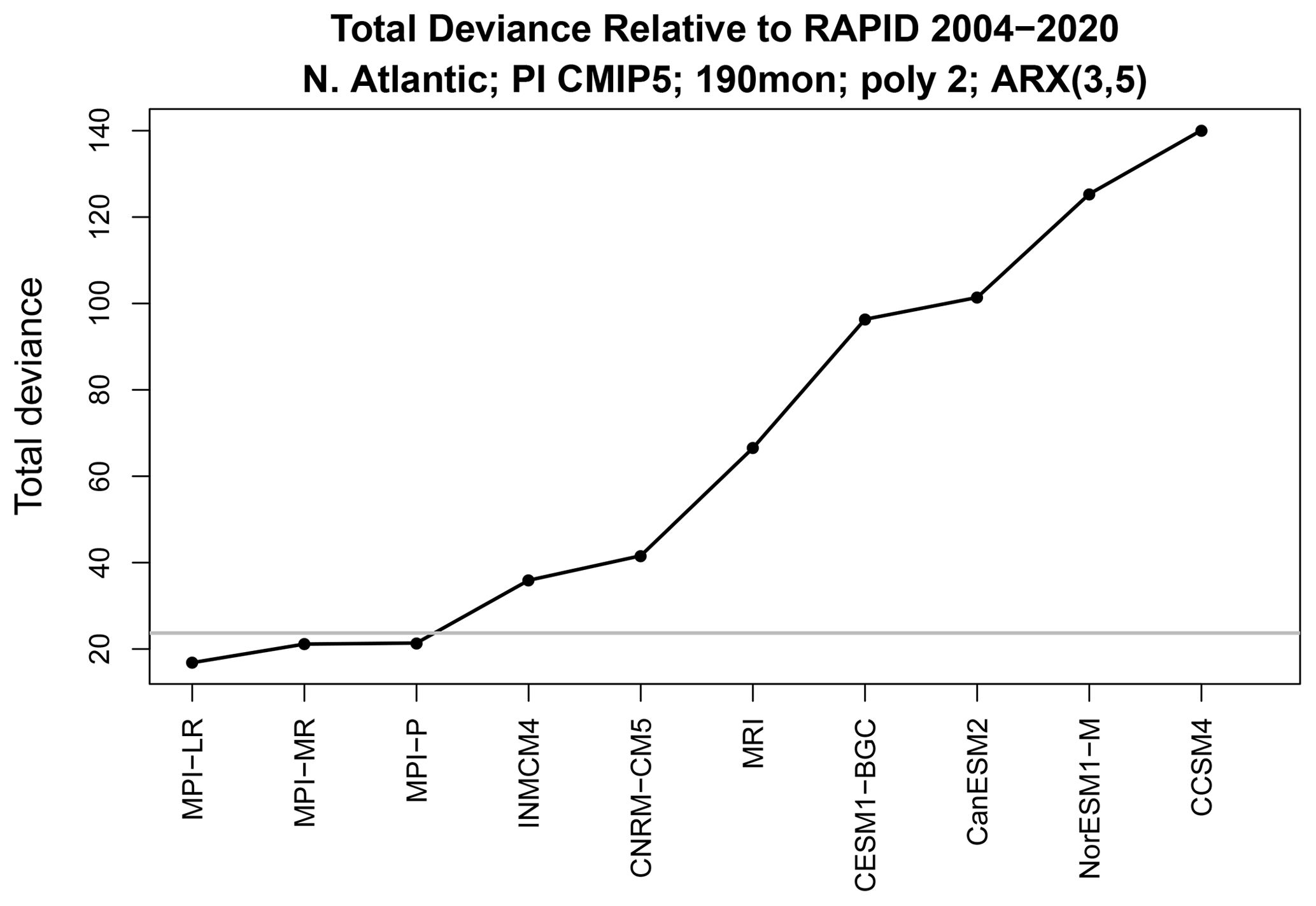
Figure 6 Total deviance between CMIP5 simulations and observational time series of the AMOC. Each time series is 190 months long and modeled by an ARX(3,5) model. The horizontal grey line shows the 5 % significance threshold.

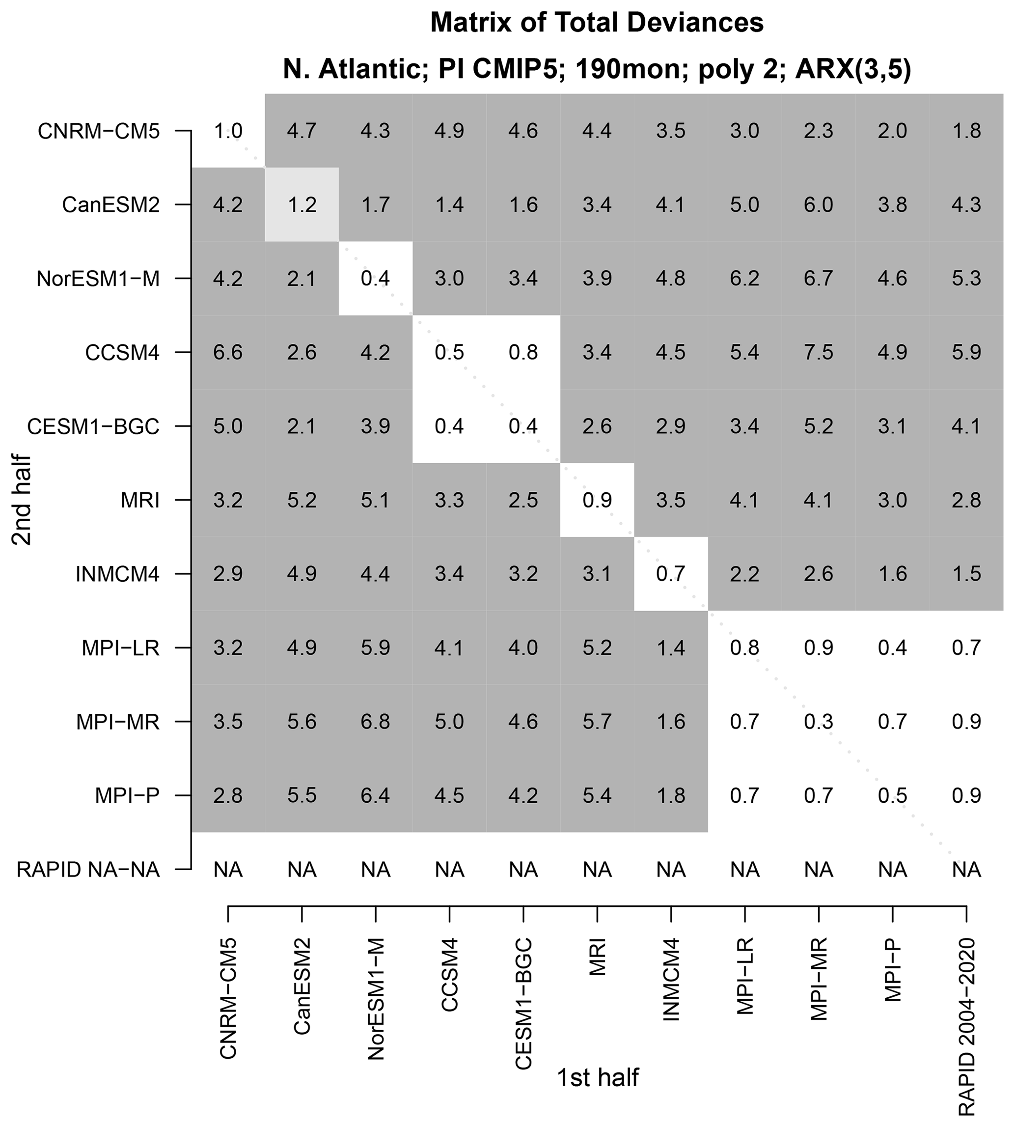
Figure 7 The total deviance between the time series shown in Fig. 2, and an independent “second-half” time series from CMIP5 models. The deviance is normalized by the 5 % significance value. Values that are insignificant, 5 % significant, and 1 % significant are indicated by no shading, light grey shading, and dark grey shading, respectively. There is no “second-half” time series for observations, but an associated bottom row is included to make the matrix square.

Although our test is rigorous, it makes asymptotic approximations whose validity may be questioned for our particular sample. One exercise for building further confidence is to compare each time series not to observations, but to time series from other models. In such a comparison, we expect deviances to be small when time series come from the same CMIP5 model. To check this, we compare each 190-month time series to an independent 190-month time series from the CMIP5 models. The resulting deviances are shown in Fig. 7. As expected, the deviances between time series from the same model, which occur along the diagonal, tend to be much smaller than those between different models (i.e., the off-diagonal elements). In fact, the diagonal elements are either insignificant or are marginally significant (i.e., $\mathrm{0.01}<p<\mathrm{0.05}$). Only one diagonal element exceeds the 5 % threshold (CanESM2), which is not serious in view of the multiple comparisons (e.g., when the null hypothesis is true, the probability of at least 1 rejection in 10 is about 4 out of 10). None of the diagonal elements exceeds the 1 % threshold.

In addition to similarities along the diagonal, there are additional similarities – different models from the same center have insignificant deviances. For instance, the two NCAR models (CCSM4 and CESM1-BGC) and the three Max Planck models (MIP-LR, MPI-MR, MPI-P) have insignificant deviances. Besides this, no other similarities are found. This example suggests that the deviance between 16-year AMOC indices could be used to decide whether two given time series came from dynamical models from the same center.

An alternative approach to summarizing these results is a dendogram. A dendogram visualizes the distance matrix in a way that makes multiple clusters easy to identify. A dendogram is constructed by linking elements together based on similarity. Here, distance is measured by total deviance $D_{{\mathrm{\Omega }}_{\mathrm{0}:\mathrm{3}}}$. At the beginning, each element is assigned to a cluster of its own. Next, the two elements with the smallest deviance are linked together, using a “leaf” whose length equals the deviance. Subsequent leaves are constructed by joining two elements with the next smallest deviance. When comparing two clusters, we assign a distance equal to the maximum deviance among all pairs of elements between the two clusters (known as the complete-linkage rule). This process repeats to produce larger clusters until all elements are in the same cluster.

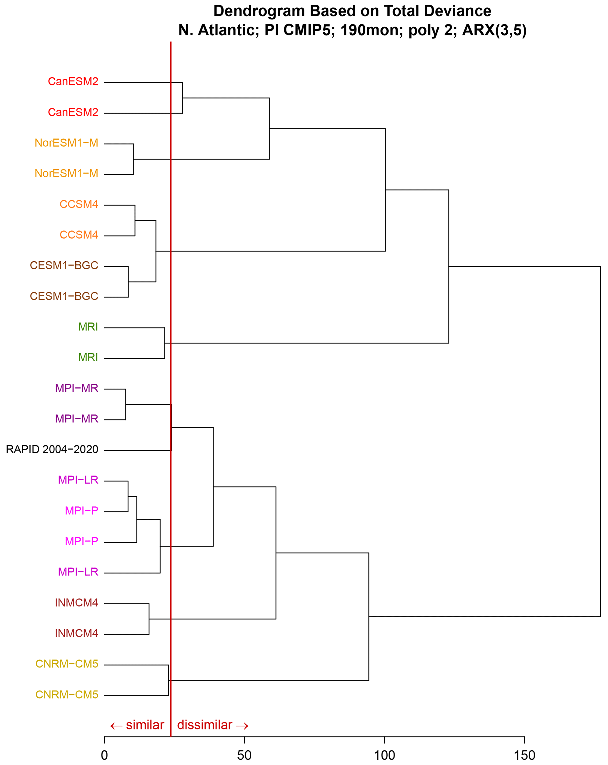
Figure 8 A dendogram showing clusters based on total deviance $D_{{\mathrm{\Omega }}_{\mathrm{0}:\mathrm{3}}}$. All time series are of length 190 months. Two independent time series from the same CMIP5 model are included in the cluster analysis. The vertical red line shows the 5 % significance level for the deviance. Leaves joined to the left of the significance line are statistically indistinguishable from each other.

The resulting dendogram is shown in Fig. 8. As can be seen, the dendogram correctly clusters time series from the same dynamical model. Observations are clustered with the MPI models, consistent with Fig. 6, and then that cluster is clustered with INMCM4 and CNRM. The other models form an entirely separate cluster. Analogous dendograms have been constructed in previous studies (for example, Knutti et al., 2013). Our cluster differs from those in previous studies in that it is based on a similarity measure with a rigorous significance test, so that statistically significant clusters can be identified rigorously.

Although significant differences from observations have been detected, the test does not tell us the nature of those differences. To gain insight into the source of the differences, we decompose the deviance as in Eq. (14) and evaluate the individual terms. The result is shown in Fig. 9. We see that only two CMIP5 models have AR deviances $D_{{\mathrm{\Omega }}_{\mathrm{1}:\mathrm{2}}}$ (green bar) that exceed the significance threshold, and these exceedances are marginal at best, suggesting that differences in AR parameters are an insignificant source of differences between ARX models. For the dynamical models that differ from observations (see Fig. 6), differences in noise are consistently significant and often dominate. Annual cycle deviances are also significant in most cases.

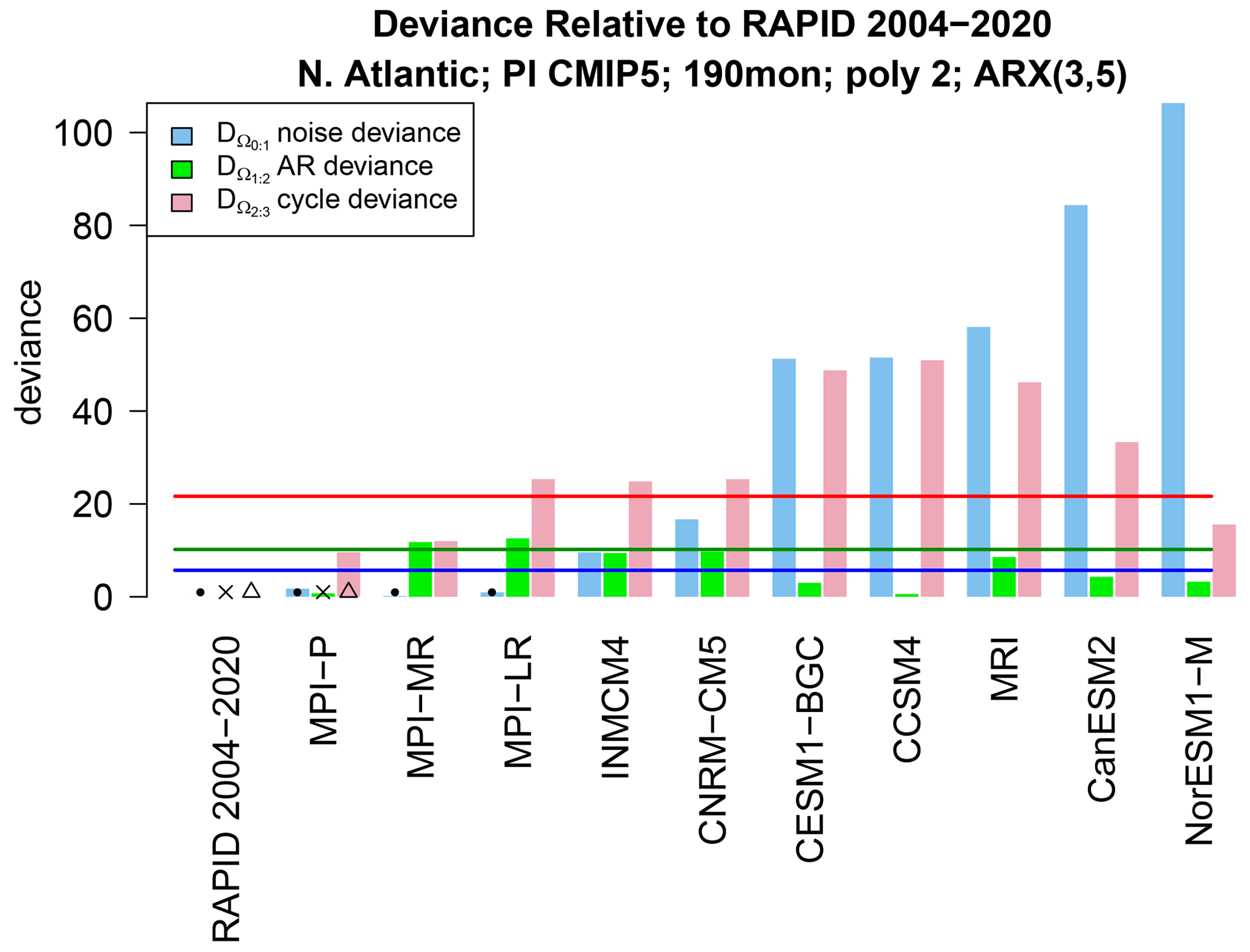
Figure 9 The AR deviance $D_{{\mathrm{\Omega }}_{\mathrm{2}:\mathrm{3}}}$ (pink bar), cycle deviance $D_{{\mathrm{\Omega }}_{\mathrm{1}:\mathrm{2}}}$ (green bar), and noise deviance $D_{{\mathrm{\Omega }}_{\mathrm{0}:\mathrm{1}}}$ (blue bar) between fitted ARX(3,5) models. The red, green, and blue lines show the corresponding significance levels at the FWER of 5 %. The dot, cross, and triangle indicate insignificant deviances. Each deviance is computed from pairs of time series each of length 190 months.

Although we have detected a significant difference in noise variance, we do not know the direction of this difference. As discussed in Sect. 4, the test for differences in noise variances is equivalent to an F test of the residuals of the ARX models. The F ratio of variances is shown in Fig. 10 and shows that CMIP5 models tend to have too little noise variance compared to observations. Differences in noise can be interpreted in a variety of ways. For instance, differences in noise imply differences in 1-month prediction errors of the ARX models. The fact that most CMIP models have too little noise variance implies that their 1-month predictions are overly confident. Alternatively, we may say models and observations have different AMOC variances after the first three lagged values have been regressed out. This constitutes a diagnostic that may be monitored during dynamical model development.

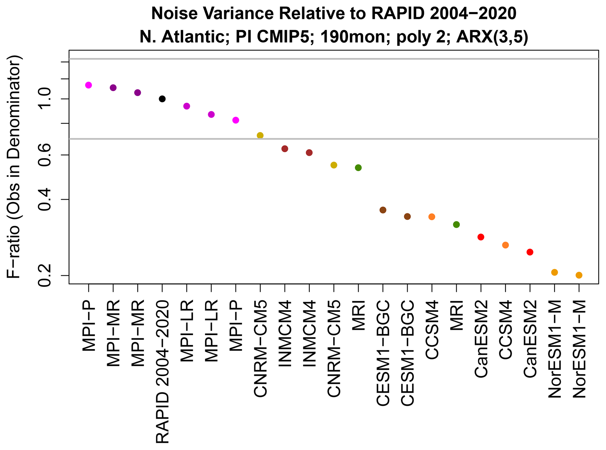
Figure 10 Ratio of noise variances between time series on the x axis and observations. Ratios less than one indicate that the CMIP5 model has less noise variance than observations. The horizontal grey lines show the upper and lower significance thresholds for rejecting equality of noise variances based on a significance level to control for a FWER of 5 %. The noise variances are each derived by fitting ARX(3,5) models to time series of length 190 months.

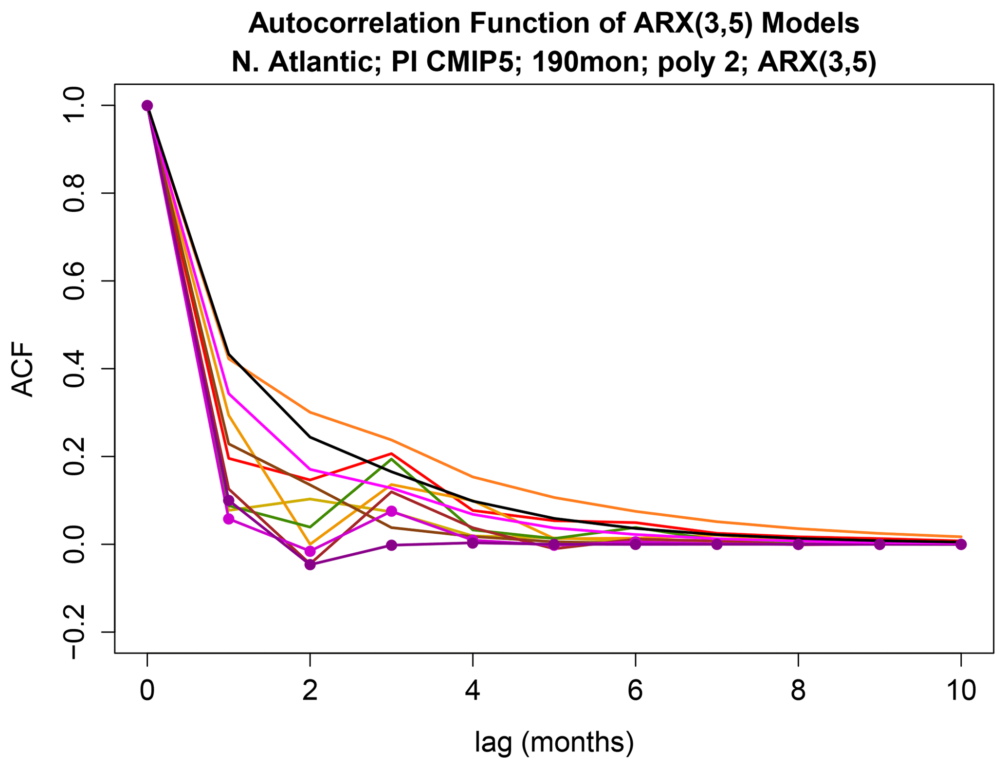
Figure 11 The autocorrelation function from each ARX(3,5) model. Dots indicate ACFs that differ significantly from that of observations at the 5 % level for FWER. The same color scheme as used in previous figures is used, including black for observations.

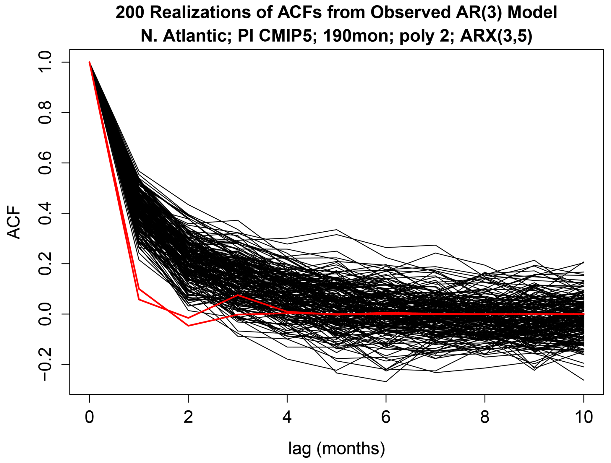
Figure 12 Two-hundred realizations of the sample autocorrelation function from the ARX(3,5) estimated from observations (black curves), and the autocorrelation function for CNRM-CM5 (red), which was found to differ significantly from observations.

Next, we consider differences in AR parameters. According to Fig. 9, only MPI-P and MPI-MR have AR parameters that differ significantly from those of observations (as indicated by the fact that the red bar crosses the red line for these models). The autocorrelation functions of the ARX(3,5) models are shown in Fig. 11. To gain insight into why the ACF for these models is identified as differing significantly from that of observations, we simulated 200 time series from the ARX(3,5) model estimated from observations and then computed the sample ACFs. The results are shown in Fig. 12. Comparing these ACFs to that of MPI-P and MPI-MR (red curves in Fig. 12) suggests that the ACFs differ from that of observations by a much faster decay.

Recall that the testing procedure stops when different noise variances are detected. Despite this, if we proceed to test differences in annual cycles, it should be recognized that the sampling distribution of the cycle deviance depends on the ratio of noise variances. Monte Carlo experiments discussed in Appendix C suggest that the chi-squared distribution provides a reasonable estimate of the 5 % significance level of $D_{{\mathrm{\Omega }}_{\mathrm{2}:\mathrm{3}}}$ in our particular data set even when Ω₁ is not true. We can therefore proceed to test equality of cycle parameters in our particular data set despite detecting differences in noise variances.

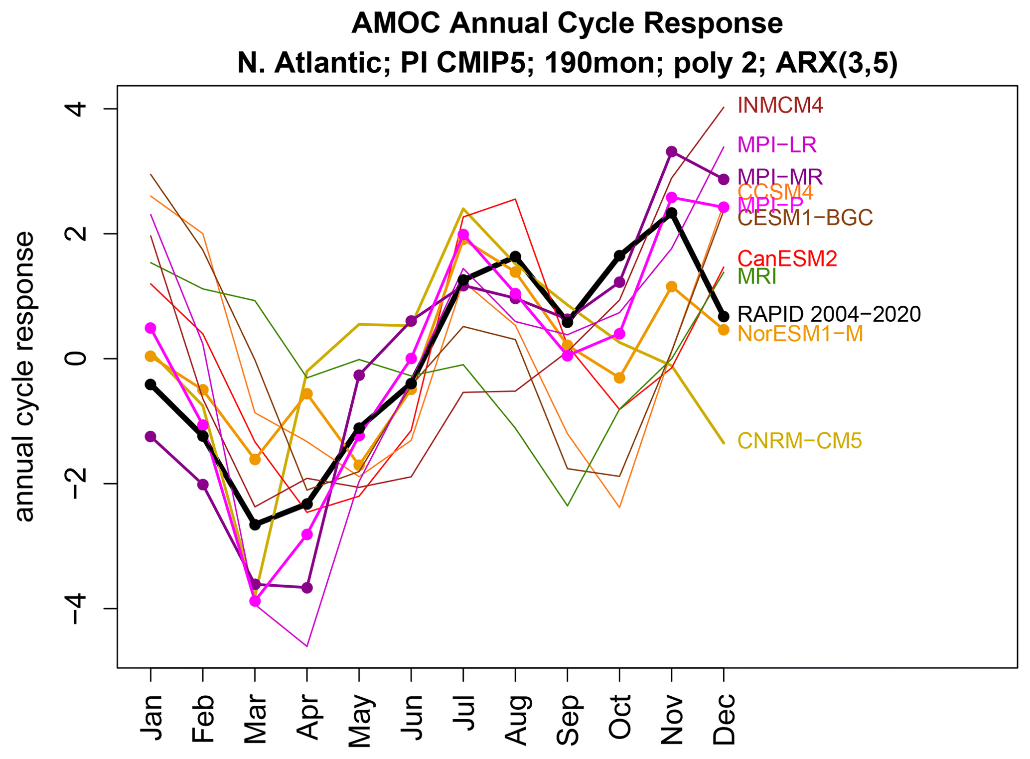
Figure 13 The annual cycle response of each ARX(3,5) model estimated from 190-month time series from CMIP5 models (colored curves) and from observations (black curve). Dots indicate annual cycles that differ significantly from that of observations at the FWER of 5 %. Note that the dots have the opposite meaning than they do in Fig. 11.

According to Fig. 9, MPI-P, MPI-MR, and NorESM1-M have annual cycles consistent with observations. To diagnose annual cycle discrepancies in the other CMIP5 models, we found it most instructive to simply plot the annual cycle response, given by Eq. (5), using Eq. (6) to convert from ARX estimates. The annual cycle response of each ARX(3,5) model is shown in Fig. 13. Dots indicate cycles that are indistinguishable from that of observations. In general, the larger the difference from the observed annual cycle, the more likely the cycles differ significantly. We draw attention to the fact that numerous studies contain plots like Fig. 13 illustrating the annual cycle for different CMIP models (e.g., Anav et al., 2013; Sanap et al., 2015; Alves et al., 2016) but without a significance test.

8 Conclusions

In this paper, we presented a test for comparing a limited class of nonstationary stochastic processes, namely, processes with deterministic signals, such as annual or diurnal cycles. The strategy was to introduce periodic deterministic terms in an autoregressive model, yielding an ARX model, and then to test for differences in the parameters. A test for equality of noise variances must precede other tests, otherwise the subsequent tests will depend on the ratio of variances, which is an unknown population parameter. This situation is similar to the t test, which tests for differences in means assuming the variances are equal. If no difference in noise variance is detected, then it is advantageous to test equality of AR parameters next, followed by equality of deterministic forcing parameters, for in this case the procedure leads to the same decision about “equality of the annual cycle” regardless of whether the hypothesis is framed in terms of forcing or response. This hierarchy of tests can be formulated such that each test is stochastically independent of the others. This stochastic independence allows the family-wise error rate of the multiple tests to be quantified rigorously.

If a difference in parameters is detected, then it is of interest to diagnose the nature of the difference. The statistic for testing differences in parameters can be decomposed into independent terms that quantify differences in noise, differences in AR parameters, and differences in deterministic forcing. Furthermore, each of these terms can be diagnosed fairly easily in a univariate setting. For instance, differences in noise variances can be characterized by the ratio of noise variances, and differences in AR parameters can be characterized by differences in autocorrelation functions associated with the ARX models.

We applied the above procedure to compare observations of the MOC from the RAPID array to CMIP5 models, treating the annual cycle as the response to deterministic forcing. The observational record is about 16 years (more precisely, 190 months) and considered sufficiently short to ignore anthropogenic climate change. To apply the procedure, the order of the AR process and the number of annual harmonics need to be chosen. We selected these parameters using a criterion called AICm, which is a generalization of Akaike's information criterion to a mixture of deterministic and random predictors. This criterion suggested choosing five annual harmonics and a third-order AR process, hence an ARX(3,5) model.

The total deviance between observations and CMIP5 models was evaluated and indicated that only three models (all from MPI) generated simulations consistent with observations. As a check on the statistical test, we compared the 190-month time series from each CMIP5 model to another independent set of time series from the CMIP5 models. We confirmed that time series from the same CMIP5 model had small deviances (the CanESM2 model had only marginally significant deviances). Interestingly, this analysis revealed that each CMIP5 model differed from every other CMIP5 model, unless the model came from the same modeling center (e.g., Max Planck or NCAR). It seems remarkable that 16 years of AMOC observations, at one latitude, is enough to distinguish CMIP5 models.

The total deviance is dominated by differences in noise variance and cycle parameters, although the relative contribution depends on CMIP5 model. Differences in AR parameters were small for our data. In other situations differences in AR parameters may play a bigger role. For models with the most extreme deviance, the noise deviance is the dominant contributor. In all cases, the noise deviance is due to the fact that models have too little noise variance compared to observations. The cycle deviance can be diagnosed by plotting the annual cycle response from each ARX model and indicating the cycles that differ significantly from observations. Although such plots have been presented in the past, this appears to be the first use of an objective criterion to identify annual cycles that differ significantly from observed annual cycles in regards to all their attributes (e.g., phases, amplitudes, frequencies) and accounting for serial correlation.

Although we have framed our procedure in terms of annual cycles, it should be recognized that the procedure applies to any deterministic function of time, including trends, exponential functions, or diurnal cycles.

Appendix A: Model formulation

Here we show how Eq. (3) can be written in the forms (7) and (8). Specifically, for time steps $t=\mathrm{1},\mathrm{\dots },N+p$, model (3) can be written in the form (7) using the identifications

$$\begin{array}{rl}\mathit{y}& =\left(\begin{array}{c}{y}_{p+\mathrm{1}}\\ y_{p+\mathrm{2}}\\ \mathrm{⋮}\\ y_{p+N}\end{array}\right),{\mathit{X}}_{\mathrm{2}}=\left(\begin{array}{cccc}{y}_p& y_{p-\mathrm{1}}& \mathrm{\dots }& y_{\mathrm{1}}\\ y_{p+\mathrm{1}}& y_p& \mathrm{\dots }& y_{\mathrm{2}}\\ \mathrm{⋮}& \mathrm{⋮}& \mathrm{\ddots }& \mathrm{⋮}\\ y_{N+p-\mathrm{1}}& y_{N+p-\mathrm{2}}& \mathrm{\dots }& y_N\end{array}\right),\\ {\mathit{\beta }}_{\mathrm{2}}& =\left(\begin{array}{c}{\mathit{\varphi }}_{\mathrm{1}}\\ {\mathit{\varphi }}_{\mathrm{2}}\\ \mathrm{⋮}\\ {\mathit{\varphi }}_p\end{array}\right),\end{array}$$

and

$$\begin{array}{}\text{(A1)}& {\mathit{X}}_{\mathrm{3}}=\left(\begin{array}{ccccc}\cos \left({\mathit{\omega }}_{\mathrm{1}}\right(p+\mathrm{1}+\mathit{\tau }\left)\right)& \sin \left({\mathit{\omega }}_{\mathrm{1}}\right(p+\mathrm{1}+\mathit{\tau }\left)\right)& \mathrm{\dots }& \cos \left({\mathit{\omega }}_H\right(p+\mathrm{1}+\mathit{\tau }\left)\right)& \sin \left({\mathit{\omega }}_H\right(p+\mathrm{1}+\mathit{\tau }\left)\right)\\ \cos \left({\mathit{\omega }}_{\mathrm{1}}\right(p+\mathrm{2}+\mathit{\tau }\left)\right)& \sin \left({\mathit{\omega }}_{\mathrm{1}}\right(p+\mathrm{2}+\mathit{\tau }\left)\right)& \mathrm{\dots }& \cos \left({\mathit{\omega }}_H\right(p+\mathrm{1}+\mathit{\tau }\left)\right)& \sin \left({\mathit{\omega }}_H\right(p+\mathrm{1}+\mathit{\tau }\left)\right)\\ \mathrm{⋮}& \mathrm{⋮}& \mathrm{\ddots }& \mathrm{⋮}& \mathrm{⋮}\\ \cos \left({\mathit{\omega }}_{\mathrm{1}}\right(p+N+\mathit{\tau }\left)\right)& \sin \left({\mathit{\omega }}_{\mathrm{1}}\right(p+N+\mathit{\tau }\left)\right)& \mathrm{\dots }& \cos \left({\mathit{\omega }}_H\right(p+\mathrm{1}+\mathit{\tau }\left)\right)& \sin \left({\mathit{\omega }}_H\right(p+\mathrm{1}+\mathit{\tau }\left)\right)\end{array}\right),\end{array}$$

where τ is a phase, and

$${\mathit{\beta }}_{\mathrm{3}}=\left(\begin{array}{c}{a}_{\mathrm{1}}\\ b_{\mathrm{1}}\\ \mathrm{⋮}\\ a_H\\ b_H\end{array}\right),\mathit{j}=\left(\begin{array}{c}\mathrm{1}\\ \mathrm{1}\\ \mathrm{⋮}\\ \mathrm{1}\end{array}\right).$$

Under these identifications, K₂=p and K₃=2H. If ω₁N is an integer multiple of 2π, then ${\mathit{X}}_{\mathrm{2}}^T{\mathit{X}}_{\mathrm{2}}$ is diagonal and ${\mathit{X}}_{\mathrm{2}}^T\mathit{j}=\mathbf{0}$, reflecting the fact that in this case the discrete Fourier functions are orthogonal and have zero mean.

Appendix B: Likelihood ratio tests and their distributions

In this Appendix, we describe the likelihood ratio tests for Ω_i+1 versus Ω_i indicated in Table 1 and show that they are independent. These results are not new and have been presented essentially by Hogg (1961). However, Hogg (1961) invokes the concept of complete sufficient statistics, which may not be familiar to many readers. The purpose of this Appendix is to summarize facts about nested likelihood ratio tests at a level that may be more accessible to climate scientists.

Under Ω₀, models (7) and (8) are independent, and hence their parameters can be estimated separately. The estimated parameters are ${\mathit{\beta }}_{\mathrm{2}},{\mathit{\beta }}_{\mathrm{2}}^{*},{\mathit{\beta }}_{\mathrm{3}},{\mathit{\beta }}_{\mathrm{3}}^{*},{\mathit{\sigma }}^{\mathrm{2}},{\mathit{\sigma }}^{*\mathrm{2}},\mathit{\mu },{\mathit{\mu }}^{*}$, the count of which is

$${\mathcal{P}}_{{\mathrm{\Omega }}_{\mathrm{0}}}=\mathrm{2}{K}_{\mathrm{2}}+\mathrm{2}{K}_{\mathrm{3}}+\mathrm{4}.$$

This is a standard problem in maximum likelihood estimation (MLE; Seber and Lee, 2003, Sect. 4.3). Let the MLEs of σ² and σ^*2 be denoted as

$${\stackrel{\mathrm{‾}}{\mathit{\sigma }}}^{\mathrm{2}}={\displaystyle \frac{Q}{N}}\text{and}{\stackrel{\mathrm{‾}}{\mathit{\sigma }}}^{*\mathrm{2}}={\displaystyle \frac{Q^{*}}{N^{*}}},$$

where Q and Q^* are the sum square errors of models (7) and (8) under Ω₀. Standard regression theory implies that the sum square errors have distributions

$${\displaystyle \frac{Q}{{\mathit{\sigma }}^{\mathrm{2}}}}\sim {\mathit{\chi }}_{N-K_{\mathrm{2}}-K_{\mathrm{3}}-\mathrm{1}}^{\mathrm{2}}\text{and}{\displaystyle \frac{Q^{*}}{{\mathit{\sigma }}^{*\mathrm{2}}}}\sim {\mathit{\chi }}_{N^{*}-K_{\mathrm{2}}-K_{\mathrm{3}}-\mathrm{1}}^{\mathrm{2}}.$$

Since Q and Q^* are independent, their ratio has a scaled F distribution under Ω₁:

$$\begin{array}{}\text{(B1)}& {\displaystyle \frac{Q}{Q^{*}}}\left({\displaystyle \frac{N^{*}-K_{\mathrm{2}}-K_{\mathrm{3}}-\mathrm{1}}{N-K_{\mathrm{2}}-K_{\mathrm{3}}-\mathrm{1}}}\right)\sim F_{N-K_{\mathrm{2}}-K_{\mathrm{3}}-\mathrm{1},N^{*}-K_{\mathrm{2}}-K_{\mathrm{3}}-\mathrm{1}}.\end{array}$$

This result provides the basis for testing Ω₁ versus Ω₀ and was used to draw the significance thresholds in Fig. 10.

The model selection criterion AICm under Ω₃ can be applied to models (7) and (8) separately, since they are independent. This criterion is Eq. (12) in DelSole and Tippett (2021a), which in our notation (for model 7) is

$$\begin{array}{}\text{(B2)}& \mathrm{\text{AICm}}=N\log {\stackrel{\mathrm{‾}}{\mathit{\sigma }}}^{\mathrm{2}}+{\displaystyle \frac{N(N+K_{\mathrm{2}}+\mathrm{1})}{N-K_{\mathrm{2}}-K_{\mathrm{3}}-\mathrm{3}}}\left(\mathrm{1}+{\displaystyle \frac{K_{\mathrm{3}}}{N-K_{\mathrm{2}}-K_{\mathrm{3}}-\mathrm{2}}}\right)\end{array}$$

(an irrelevant additive term equal to Nlog 2π has been dropped).

Under ${\mathrm{\Omega }}_{\mathrm{1}},{\mathrm{\Omega }}_{\mathrm{2}},{\mathrm{\Omega }}_{\mathrm{3}}$, models (7) and (8) have a common variance. In this case, Eqs. (7) and (8) can be combined as

$$\mathbb{Y}=\mathbb{X}\mathbb{B}+\mathbb{E},$$

where

$$\mathbb{Y}=\left(\begin{array}{c}\mathit{y}\\ {\mathit{y}}^{*}\end{array}\right),\mathbb{E}=\left(\begin{array}{c}\mathit{ϵ}\\ {\mathit{ϵ}}^{*}\end{array}\right)$$

and where 𝕏 and 𝔹 have the following identifications under ${\mathrm{\Omega }}_{\mathrm{1}},{\mathrm{\Omega }}_{\mathrm{2}},{\mathrm{\Omega }}_{\mathrm{3}}$:

$$\begin{array}{c}{\displaystyle }{\mathrm{\Omega }}_{\mathrm{1}}:\mathbb{X}=\left(\begin{array}{cccccc}{\mathit{X}}_{\mathrm{2}}& {\mathit{X}}_{\mathrm{3}}& \mathit{j}& \mathbf{0}& \mathbf{0}& \mathbf{0}\\ \mathbf{0}& \mathbf{0}& \mathbf{0}& {\mathit{X}}_{\mathrm{2}}^{*}& {\mathit{X}}_{\mathrm{3}}^{*}& {\mathit{j}}^{*}\end{array}\right),\mathbb{B}=\left(\begin{array}{c}{\mathit{\beta }}_{\mathrm{2}}\\ {\mathit{\beta }}_{\mathrm{3}}\\ \mathit{\mu }\\ {\mathit{\beta }}_{\mathrm{2}}^{*}\\ {\mathit{\beta }}_{\mathrm{3}}^{*}\\ {\mathit{\mu }}^{*}\end{array}\right)\\ {\displaystyle }{\mathrm{\Omega }}_{\mathrm{2}}:\mathbb{X}=\left(\begin{array}{ccccc}{\mathit{X}}_{\mathrm{2}}& {\mathit{X}}_{\mathrm{3}}& \mathit{j}& \mathbf{0}& \mathbf{0}\\ {\mathit{X}}_{\mathrm{2}}^{*}& \mathbf{0}& \mathbf{0}& {\mathit{X}}_{\mathrm{3}}^{*}& {\mathit{j}}^{*}\end{array}\right),\mathbb{B}=\left(\begin{array}{c}{\mathit{\beta }}_{\mathrm{2}}\\ {\mathit{\beta }}_{\mathrm{3}}\\ \mathit{\mu }\\ {\mathit{\beta }}_{\mathrm{3}}^{*}\\ {\mathit{\mu }}^{*}\end{array}\right)\\ {\displaystyle }{\mathrm{\Omega }}_{\mathrm{3}}:\mathbb{X}=\left(\begin{array}{cccc}{\mathit{X}}_{\mathrm{2}}& {\mathit{X}}_{\mathrm{3}}& \mathit{j}& \mathbf{0}\\ {\mathit{X}}_{\mathrm{2}}^{*}& {\mathit{X}}_{\mathrm{3}}^{*}& \mathbf{0}& {\mathit{j}}^{*}\end{array}\right),\mathbb{B}=\left(\begin{array}{c}{\mathit{\beta }}_{\mathrm{2}}\\ {\mathit{\beta }}_{\mathrm{3}}\\ \mathit{\mu }\\ {\mathit{\mu }}^{*}\end{array}\right)\end{array}$$

Each estimation problem requires estimation of 𝔹 and the common variance σ², and hence the numbers of parameters estimated under ${\mathrm{\Omega }}_{\mathrm{1}},{\mathrm{\Omega }}_{\mathrm{2}},{\mathrm{\Omega }}_{\mathrm{3}}$ are, respectively,

$$\begin{array}{ll}{\displaystyle }{\mathcal{P}}_{{\mathrm{\Omega }}_{\mathrm{1}}}& {\displaystyle }=\mathrm{2}{K}_{\mathrm{2}}+\mathrm{2}{K}_{\mathrm{3}}+\mathrm{3}\\ {\displaystyle }{\mathcal{P}}_{{\mathrm{\Omega }}_{\mathrm{2}}}& {\displaystyle }=K_{\mathrm{2}}+\mathrm{2}{K}_{\mathrm{3}}+\mathrm{3}\\ {\displaystyle }{\mathcal{P}}_{{\mathrm{\Omega }}_{\mathrm{3}}}& {\displaystyle }=K_{\mathrm{2}}+K_{\mathrm{3}}+\mathrm{3}.\end{array}$$

The sum square errors of the model estimated under Ω_i (for i≥1) can be written as the quadratic form

$$\begin{array}{}\text{(B3)}& Q_{{\mathrm{\Omega }}_i}={\mathbb{Y}}^T\left(\mathbf{I}-{\mathbf{P}}_{{\mathrm{\Omega }}_i}\right)\mathbb{Y},\end{array}$$

where ${\mathbf{P}}_{{\mathrm{\Omega }}_i}$ is an orthogonal projection matrix appropriate to hypothesis Ω_i,

$${\mathbf{P}}_{{\mathrm{\Omega }}_i}={\mathbb{X}}_{{\mathrm{\Omega }}_i}{\left({\mathbb{X}}_{{\mathrm{\Omega }}_i}^T{\mathbb{X}}_{{\mathrm{\Omega }}_i}\right)}^{-\mathrm{1}}{\mathbb{X}}_{{\mathrm{\Omega }}_i}^T.$$

The maximum likelihood estimate of σ² under Ω_i for i≥1 is denoted as

$${\stackrel{\mathrm{‾}}{\mathit{\sigma }}}_{{\mathrm{\Omega }}_i}^{\mathrm{2}}={\displaystyle \frac{Q_{{\mathrm{\Omega }}_i}}{N+N^{*}}}.$$

In general, $Q_{{\mathrm{\Omega }}_{\mathrm{1}}}\le Q_{{\mathrm{\Omega }}_{\mathrm{2}}}\le Q_{{\mathrm{\Omega }}_{\mathrm{3}}}$ and ${\stackrel{\mathrm{‾}}{\mathit{\sigma }}}_{{\mathrm{\Omega }}_{\mathrm{1}}}^{\mathrm{2}}\le {\stackrel{\mathrm{‾}}{\mathit{\sigma }}}_{{\mathrm{\Omega }}_{\mathrm{2}}}^{\mathrm{2}}\le {\stackrel{\mathrm{‾}}{\mathit{\sigma }}}_{{\mathrm{\Omega }}_{\mathrm{3}}}^{\mathrm{2}}.$

If Ω_i is true, then standard regression theory gives

$${\displaystyle \frac{Q_{{\mathrm{\Omega }}_i}}{{\mathit{\sigma }}^{\mathrm{2}}}}{\displaystyle }\sim {\mathit{\chi }}_{{\mathit{\nu }}_i}^{\mathrm{2}},$$

with the degrees of freedom

$${\mathit{\nu }}_i=N+N^{*}-{\mathcal{P}}_{{\mathrm{\Omega }}_i}+\mathrm{1}$$

(one is added because σ is counted in 𝒫 but not in ν).

Testing the hypotheses in Table 1 requires knowing the distribution of ratios of $Q_{{\mathrm{\Omega }}_{\mathrm{1}}},Q_{{\mathrm{\Omega }}_{\mathrm{2}}},Q_{{\mathrm{\Omega }}_{\mathrm{3}}}$. These distributions follow from the identity

$$\begin{array}{}\text{(B4)}& \mathbf{I}-{\mathbf{P}}_{{\mathrm{\Omega }}_{\mathrm{3}}}=\left(\mathbf{I}-{\mathbf{P}}_{{\mathrm{\Omega }}_{\mathrm{1}}}\right)+\left({\mathbf{P}}_{{\mathrm{\Omega }}_{\mathrm{1}}}-{\mathbf{P}}_{{\mathrm{\Omega }}_{\mathrm{2}}}\right)+\left({\mathbf{P}}_{{\mathrm{\Omega }}_{\mathrm{2}}}-{\mathbf{P}}_{{\mathrm{\Omega }}_{\mathrm{3}}}\right).\end{array}$$

Specifically, the projection matrices are idempotent and satisfy

$$\begin{array}{}\text{(B5)}& {\mathbf{P}}_{{\mathrm{\Omega }}_{i+j}}{\mathbf{P}}_{{\mathrm{\Omega }}_i}={\mathbf{P}}_{{\mathrm{\Omega }}_i}{\mathbf{P}}_{{\mathrm{\Omega }}_{i+j}}={\mathbf{P}}_{{\mathrm{\Omega }}_{i+j}}\text{for }i\ge \mathrm{1},j\ge \mathrm{0}.\end{array}$$

This identity can be seen from the fact that the columns of ${\mathbb{X}}_{{\mathrm{\Omega }}_{i+j}}$ are a linear combination of the columns of ${\mathbb{X}}_{{\mathrm{\Omega }}_i}$, and hence there exists a matrix ℂ such that

$${\mathbb{X}}_{{\mathrm{\Omega }}_{i+j}}={\mathbb{X}}_{{\mathrm{\Omega }}_i}\mathbb{C}.$$

Therefore

$$\begin{array}{ll}{\displaystyle }{\mathbf{P}}_{{\mathrm{\Omega }}_i}{\mathbf{P}}_{{\mathrm{\Omega }}_{i+j}}=& {\displaystyle }{\mathbb{X}}_{{\mathrm{\Omega }}_i}{\left({\mathbb{X}}_{{\mathrm{\Omega }}_i}^T{\mathbb{X}}_{{\mathrm{\Omega }}_i}\right)}^{-\mathrm{1}}{\mathbb{X}}_{{\mathrm{\Omega }}_i}^T{\mathbb{X}}_{{\mathrm{\Omega }}_{i+j}}\\ {\displaystyle }& {\displaystyle }\cdot {\left({\mathbb{X}}_{{\mathrm{\Omega }}_{i+j}}^T{\mathbb{X}}_{{\mathrm{\Omega }}_{i+j}}\right)}^{-\mathrm{1}}{\mathbb{X}}_{{\mathrm{\Omega }}_{i+j}}^T\\ {\displaystyle }=& {\displaystyle }{\mathbb{X}}_{{\mathrm{\Omega }}_i}{\left({\mathbb{X}}_{{\mathrm{\Omega }}_i}^T{\mathbb{X}}_{{\mathrm{\Omega }}_i}\right)}^{-\mathrm{1}}{\mathbb{X}}_{{\mathrm{\Omega }}_i}^T{\mathbb{X}}_{{\mathrm{\Omega }}_i}\mathbb{C}\\ {\displaystyle }& {\displaystyle }\cdot {\left({\mathbb{X}}_{{\mathrm{\Omega }}_{i+j}}^T{\mathbb{X}}_{{\mathrm{\Omega }}_{i+j}}\right)}^{-\mathrm{1}}{\mathbb{X}}_{{\mathrm{\Omega }}_{i+j}}^T\\ {\displaystyle }=& {\displaystyle }{\mathbb{X}}_{{\mathrm{\Omega }}_i}\mathbb{C}{\left({\mathbb{X}}_{{\mathrm{\Omega }}_{i+j}}^T{\mathbb{X}}_{{\mathrm{\Omega }}_{i+j}}\right)}^{-\mathrm{1}}{\mathbb{X}}_{{\mathrm{\Omega }}_{i+j}}^T\\ {\displaystyle }=& {\displaystyle }{\mathbb{X}}_{{\mathrm{\Omega }}_{i+j}}{\left({\mathbb{X}}_{{\mathrm{\Omega }}_{i+j}}^T{\mathbb{X}}_{{\mathrm{\Omega }}_{i+j}}\right)}^{-\mathrm{1}}{\mathbb{X}}_{{\mathrm{\Omega }}_{i+j}}^T\\ {\displaystyle }=& {\displaystyle }{\mathbf{P}}_{{\mathrm{\Omega }}_{i+j}}.\end{array}$$

A similar proof shows that ${\mathbf{P}}_{{\mathrm{\Omega }}_{i+j}}{\mathbf{P}}_{{\mathrm{\Omega }}_i}={\mathbf{P}}_{{\mathrm{\Omega }}_{i+j}}$.

As a result of Eq. (B5), the product of any pair of

$$\left(\mathbf{I}-{\mathbf{P}}_{{\mathrm{\Omega }}_{\mathrm{1}}}\right),\left({\mathbf{P}}_{{\mathrm{\Omega }}_{\mathrm{1}}}-{\mathbf{P}}_{{\mathrm{\Omega }}_{\mathrm{2}}}\right),\left({\mathbf{P}}_{{\mathrm{\Omega }}_{\mathrm{2}}}-{\mathbf{P}}_{{\mathrm{\Omega }}_{\mathrm{3}}}\right)$$

vanishes. Multiplying Eq. (B4) by 𝕐 on the left and right to produce quadratic forms gives

$$\begin{array}{}\text{(B6)}& Q_{{\mathrm{\Omega }}_{\mathrm{3}}}=Q_{{\mathrm{\Omega }}_{\mathrm{1}}}+\left(Q_{{\mathrm{\Omega }}_{\mathrm{2}}}-Q_{{\mathrm{\Omega }}_{\mathrm{1}}}\right)+\left(Q_{{\mathrm{\Omega }}_{\mathrm{3}}}-Q_{{\mathrm{\Omega }}_{\mathrm{2}}}\right).\end{array}$$

It follows from Cochran's theorem (Seber, 2015, Theorem 4.1) that

$$\begin{array}{}\text{(B7)}& {\displaystyle \frac{Q_{{\mathrm{\Omega }}_{\mathrm{1}}}}{{\mathit{\sigma }}^{\mathrm{2}}}},{\displaystyle \frac{Q_{{\mathrm{\Omega }}_{\mathrm{2}}}-Q_{{\mathrm{\Omega }}_{\mathrm{1}}}}{{\mathit{\sigma }}^{\mathrm{2}}}},{\displaystyle \frac{Q_{{\mathrm{\Omega }}_{\mathrm{3}}}-Q_{{\mathrm{\Omega }}_{\mathrm{2}}}}{{\mathit{\sigma }}^{\mathrm{2}}}}\end{array}$$

are distributed as independent chi square with respective degrees of freedom

$${\mathit{\nu }}_{{\mathrm{\Omega }}_{\mathrm{1}}},{\mathit{\nu }}_{{\mathrm{\Omega }}_{\mathrm{2}}}-{\mathit{\nu }}_{{\mathrm{\Omega }}_{\mathrm{1}}},{\mathit{\nu }}_{{\mathrm{\Omega }}_{\mathrm{3}}}-{\mathit{\nu }}_{{\mathrm{\Omega }}_{\mathrm{2}}}.$$

Therefore, if Ω_i+j is true, then

$$\begin{array}{}\text{(B8)}& \begin{array}{rl}& \left({\displaystyle \frac{Q_{{\mathrm{\Omega }}_{i+j}}-Q_{{\mathrm{\Omega }}_i}}{Q_{{\mathrm{\Omega }}_i}}}\right)\left({\displaystyle \frac{{\mathit{\nu }}_i}{{\mathit{\nu }}_{i+j}-{\mathit{\nu }}_i}}\right)\sim F_{{\mathit{\nu }}_{i+j}-{\mathit{\nu }}_i,{\mathit{\nu }}_i}\\ & \text{for }i\ge \mathrm{1},j\ge \mathrm{1}.\end{array}\end{array}$$

This result provides the basis for testing $Q_{{\mathrm{\Omega }}_{i+j}}$ relative to $Q_{{\mathrm{\Omega }}_i}$ for $i\ge \mathrm{1},j\ge \mathrm{1}$.

The test derived from Eq. (B8) is a standard analysis of variance (ANOVA) test. For instance, in R, the tests for pairwise comparisons of ${\mathrm{\Omega }}_{\mathrm{1}},{\mathrm{\Omega }}_{\mathrm{2}},{\mathrm{\Omega }}_{\mathrm{3}}$ can be performed using the commands anova(Model2, Model1) and anova(Model3, Model2), where Model1, Model2, Model3 are the model fits from lm under ${\mathrm{\Omega }}_{\mathrm{1}},{\mathrm{\Omega }}_{\mathrm{2}},{\mathrm{\Omega }}_{\mathrm{3}}$, respectively. Unfortunately, comparison of Ω₀ and Ω₁ is not part of the standard decomposition because ANOVA assumes that variables come from populations with the same variance σ². If the populations have different variances, then the F statistic in Eq. (B8) would not have an F distribution and would depend on the population variance ratio. Therefore, the anova command in R does not handle the test for equality of noise variances, and in fact assumes equality of noise variances. Although the comparison between Ω₀ and Ω₁ is not part a standard analysis of variance table, it can be included in a deviance decomposition.

A further point is that comparing three hypotheses ${\mathrm{\Omega }}_{\mathrm{1}},{\mathrm{\Omega }}_{\mathrm{2}},{\mathrm{\Omega }}_{\mathrm{3}}$ with the command anova(Model3, Model2, Model1) is not equivalent to testing each model pairwise (for instance, different F values are produced). The reason for this is that when comparing more than two models, it is convention to compute the denominator for the F statistic in Eq. (B8) using the least restrictive model, namely, $Q_{{\mathrm{\Omega }}_{\mathrm{1}}}/{\mathit{\nu }}_{\mathrm{1}}$ rather than $Q_{{\mathrm{\Omega }}_i}/{\mathit{\nu }}_i$. Unfortunately, this convention leads to F statistics that are not mutually stochastically independent, as noted by Hogg (1961). In contrast, comparing models pairwise leads to F statistics that are mutually stochastically independent, as we show below using a more elementary proof than that of Hogg (1961).

To prove the independence of the F statistics in the hierarchy, we focus on the likelihoods. The maximized likelihoods for Eqs. (7) and (8) are, respectively,

$$L=(\mathrm{2}\mathit{\pi }e{\stackrel{\mathrm{‾}}{\mathit{\sigma }}}^{\mathrm{2}}{)}^{-N/\mathrm{2}}\text{and}{L}^{*}=(\mathrm{2}\mathit{\pi }e{\stackrel{\mathrm{‾}}{\mathit{\sigma }}}^{*\mathrm{2}}{)}^{-N^{*}/\mathrm{2}}.$$

Since Eqs. (7) and (8) are independent, the total likelihood for Ω₀ is

$$L_{{\mathrm{\Omega }}_{\mathrm{0}}}=L{L}^{*}.$$

The maximized likelihood under Ω_i for i=1, 2, 3 is

$$L_{{\mathrm{\Omega }}_i}={\left(\mathrm{2}\mathit{\pi }e{\stackrel{\mathrm{‾}}{\mathit{\sigma }}}_{{\mathrm{\Omega }}_i}^{\mathrm{2}}\right)}^{-(N+N^{*})/\mathrm{2}}\text{for }i\ge \mathrm{1}.$$

Therefore,

$$\begin{array}{}\text{(B9)}& {\displaystyle \frac{L_{{\mathrm{\Omega }}_{i+\mathrm{1}}}}{L_{{\mathrm{\Omega }}_i}}}={\left({\displaystyle \frac{Q_{{\mathrm{\Omega }}_{i+\mathrm{1}}}}{Q_{{\mathrm{\Omega }}_i}}}\right)}^{-(N+N^{*})/\mathrm{2}}\text{for }i\ge \mathrm{1}\end{array}$$

and

$$\begin{array}{}\text{(B10)}& {\displaystyle \frac{L_{{\mathrm{\Omega }}_{\mathrm{1}}}}{L_{{\mathrm{\Omega }}_{\mathrm{0}}}}}={\displaystyle \frac{{\left(\frac{Q_{{\mathrm{\Omega }}_{\mathrm{1}}}}{N+N^{*}}\right)}^{-(N+N^{*})/\mathrm{2}}}{{\left(\frac{Q}{N}\right)}^{-N/\mathrm{2}}{\left(\frac{Q^{*}}{N^{*}}\right)}^{-N^{*}/\mathrm{2}}}}.\end{array}$$

The likelihood ratio (B9) can be written equivalently as

$${\displaystyle \frac{L_{{\mathrm{\Omega }}_{i+\mathrm{1}}}}{L_{{\mathrm{\Omega }}_i}}}={\left(\mathrm{1}+{\displaystyle \frac{Q_{{\mathrm{\Omega }}_{i+j}}-Q_{{\mathrm{\Omega }}_i}}{Q_{{\mathrm{\Omega }}_i}}}\right)}^{-(N+N^{*})/\mathrm{2}}\text{for }i\ge \mathrm{1}.$$

Also, using $Q_{{\mathrm{\Omega }}_{\mathrm{1}}}=Q+Q^{*}$, the likelihood ratio (B10) can be written equivalently in terms of the variance ratio $r=Q/Q^{*}$ as

$${\displaystyle \frac{L_{{\mathrm{\Omega }}_{\mathrm{1}}}}{L_{{\mathrm{\Omega }}_{\mathrm{0}}}}}=f\left(r\right)={\left(\mathrm{1}+\mathrm{1}/r\right)}^{-N/\mathrm{2}}{\left(\mathrm{1}+r\right)}^{-N^{*}/\mathrm{2}}\left({\displaystyle \frac{N^{-\frac{N}{\mathrm{2}}}{N^{*}}^{-\frac{N^{*}}{\mathrm{2}}}}{(N+N^{*}{)}^{-(N+N^{*})/\mathrm{2}}}}\right).$$

The likelihood ratio for testing Ω₃ versus Ω₀ can be written in the factored form

$$\begin{array}{}\text{(B11)}& {\displaystyle \frac{L_{{\mathrm{\Omega }}_{\mathrm{3}}}}{L_{{\mathrm{\Omega }}_{\mathrm{0}}}}}={\displaystyle \frac{L_{{\mathrm{\Omega }}_{\mathrm{1}}}}{L_{{\mathrm{\Omega }}_{\mathrm{0}}}}}{\displaystyle \frac{L_{{\mathrm{\Omega }}_{\mathrm{2}}}}{L_{{\mathrm{\Omega }}_{\mathrm{1}}}}}{\displaystyle \frac{L_{{\mathrm{\Omega }}_{\mathrm{3}}}}{L_{{\mathrm{\Omega }}_{\mathrm{2}}}}}.\end{array}$$

Independence of Eq. (B7) implies independence of the numerators of $L_{{\mathrm{\Omega }}_{\mathrm{1}}}{L}_{{\mathrm{\Omega }}_{\mathrm{2}}}{L}_{{\mathrm{\Omega }}_{\mathrm{3}}}$. However, this does not imply that the ratios in Eq. (B11) are independent. To show independence of the ratios, we write the product in the form

$$\begin{array}{}\text{(B12)}& {\left({\displaystyle \frac{L_{{\mathrm{\Omega }}_{\mathrm{3}}}}{L_{{\mathrm{\Omega }}_{\mathrm{0}}}}}\right)}^{-\mathrm{2}/(N+N^{*})}=f\left({\displaystyle \frac{a}{b}}\right)g\left({\displaystyle \frac{c}{a+b}}\right)g\left({\displaystyle \frac{d}{a+b+c}}\right),\end{array}$$

where $g\left(x\right)=\mathrm{1}+x$ and $a,b,c,d$ are independent and defined as

$$a=Q^{*},b=Q,c=Q_{{\mathrm{\Omega }}_{\mathrm{2}}}-Q_{{\mathrm{\Omega }}_{\mathrm{1}}},d=Q_{{\mathrm{\Omega }}_{\mathrm{3}}}-Q_{{\mathrm{\Omega }}_{\mathrm{2}}}.$$

For each consecutive pair of products in Eq. (B12), the denominator on the right is the sum of the numerator and denominator on the left. Lukacs (1955) proved that if w and z are independent and have gamma distributions with the same scale parameter, then $w/z$ and w+z are also independent. Since the chi-squared distribution is a gamma distribution with scale parameter 2, Lukacs' theorem implies that the factors in Eq. (B12) are independent. This proof can be generalized to any number of nested hypotheses. The above decomposition is also derived in Hogg (1961) based on an independence theorem associated with complete sufficient statistics.

Note that if equality of noise variance Ω₀ were not assumed in ${\mathrm{\Omega }}_{\mathrm{1}},{\mathrm{\Omega }}_{\mathrm{2}},{\mathrm{\Omega }}_{\mathrm{3}}$, the sampling distributions would depend on the ratio of noise variances and not have F distributions. This situation is similar to the Behrens–Fisher problem, to which our problem would reduce if X₂=0 and X₃=0 and the hypothesis $\mathit{\mu }={\mathit{\mu }}^{*}$ were included in the hierarchy.

We end by defining the associated deviance statistics and their distributions. The deviance is defined as

$$D_{{\mathrm{\Omega }}_{i:i+k}}=-\mathrm{2}\log L_{{\mathrm{\Omega }}_{i+k}}+\mathrm{2}\log L_{{\mathrm{\Omega }}_i}.$$

In particular,

$$\begin{array}{ll}{\displaystyle }{D}_{{\mathrm{\Omega }}_{\mathrm{0}:\mathrm{1}}}& {\displaystyle }=-\mathrm{2}\log f(Q/Q^{*}),\\ {\displaystyle }{D}_{{\mathrm{\Omega }}_{i:i+\mathrm{1}}}& {\displaystyle }=(N+N^{*})\log \left({\displaystyle \frac{Q_{{\mathrm{\Omega }}_{i+\mathrm{1}}}}{Q_{{\mathrm{\Omega }}_i}}}\right)\text{for }i\ge \mathrm{1}.\end{array}$$

It follows trivially that

$$\begin{array}{}\text{(B13)}& D_{{\mathrm{\Omega }}_{\mathrm{0}:\mathrm{3}}}=D_{{\mathrm{\Omega }}_{\mathrm{0}:\mathrm{1}}}+D_{{\mathrm{\Omega }}_{\mathrm{1}:\mathrm{2}}}+D_{{\mathrm{\Omega }}_{\mathrm{2}:\mathrm{3}}}.\end{array}$$

The terms on the right-hand side are independent because of the independence of the factors in Eq. (B11).

The sampling distribution of $D_{{\mathrm{\Omega }}_{i:i+\mathrm{1}}}$ when Ω_i+1 is true can be derived from Eq. (B1) for i=0 and from Eq. (B8) for i≥1. It turns out that Monte Carlo techniques provide an easier way to estimate the significance threshold for $D_{{\mathrm{\Omega }}_{\mathrm{0}:\mathrm{1}}}$. In this approach, we draw 1000 random samples from

$$r^{\prime }=F_{N-K_{\mathrm{2}}-K_{\mathrm{3}}-\mathrm{1},N^{*}-K_{\mathrm{2}}-K_{\mathrm{3}}-\mathrm{1}}\left({\displaystyle \frac{N-K_{\mathrm{2}}-K_{\mathrm{3}}-\mathrm{1}}{N^{*}-K_{\mathrm{2}}-K_{\mathrm{3}}-\mathrm{1}}}\right)$$

and then compute 1000 realizations of

$$D_{{\mathrm{\Omega }}_{\mathrm{0}:\mathrm{1}}}=-\mathrm{2}\log f\left(r^{\prime }\right).$$

The 95th percentile is then an estimate of the 5 % significance threshold. This Monte Carlo estimate is fast because the F distribution is sampled directly. The (1−α)100 % significance threshold of $D_{{\mathrm{\Omega }}_{i:i+\mathrm{1}}}$ can be derived from Eq. (B8) as

$$\begin{array}{}\text{(B14)}& D_{{\mathrm{\Omega }}_{i:i+\mathrm{1}}}^{\left(\mathit{\alpha }\right)}=(N+N^{*})\log \left(\mathrm{1}+F_{\mathit{\alpha },{\mathit{\nu }}_{i+\mathrm{1}}-{\mathit{\nu }}_i,{\mathit{\nu }}_i}\left({\displaystyle \frac{{\mathit{\nu }}_{i+\mathrm{1}}-{\mathit{\nu }}_i}{{\mathit{\nu }}_i}}\right)\right).\end{array}$$

A less accurate but more convenient approach is to use the fact that, when Ω_i+j is true, the deviance has asymptotic distribution

$$D_{{\mathrm{\Omega }}_{i:i+\mathrm{1}}}\sim {\mathit{\chi }}_{{\mathcal{P}}_i-{\mathcal{P}}_{i+\mathrm{1}}}^{\mathrm{2}}.$$

Because the factors $L_{{\mathrm{\Omega }}_{\mathrm{1}}}/L_{{\mathrm{\Omega }}_{\mathrm{0}}},L_{{\mathrm{\Omega }}_{\mathrm{2}}}/L_{{\mathrm{\Omega }}_{\mathrm{1}}},L_{{\mathrm{\Omega }}_{\mathrm{3}}}/L_{{\mathrm{\Omega }}_{\mathrm{2}}}$ are stochastically independent, it is straightforward to control the family-wise error rate of the test. For instance, for a hierarchy with J tests, a family-wise error rate (FWER) of α can be achieved by setting the type-I error of each test to $\mathrm{1}-(\mathrm{1}-\mathit{\alpha }{)}^{\mathrm{1}/J}$. Of course, other choices for the individual type-I error rates could be selected to give the same FWER, but there is little reason to prefer one test to have a higher type-I error rate than the others.

Appendix C: Monte Carlo experiments

In this Appendix, we quantify the sensitivity of the significance threshold of $D_{{\mathrm{\Omega }}_{\mathrm{2}:\mathrm{3}}}$ to differences in noise variances. To do this, we take the best fit ARX(3,5) model for each CMIP5 model (i.e., the maximum likelihood estimates under Ω₀) and compare it to the same model except with a noise variance 5 times larger (hence Ω₁ is false). A variance ratio of 5 was chosen because it is the most extreme variance ratio from Fig. 10. We generate time series of length 190 from both ARX(3,5) models, evaluate $D_{{\mathrm{\Omega }}_{\mathrm{2}:\mathrm{3}}}$, repeat 2000 times, and identify the 95th percentiles. The 95th percentile is chosen merely as a reference and does not correspond to the actual significance level of the hierarchical test.

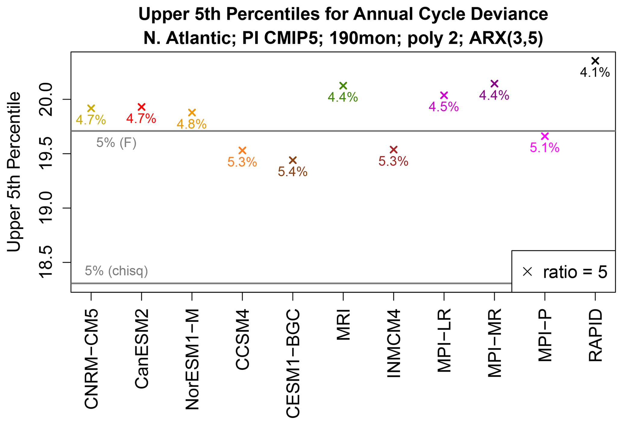
Figure C1 Upper 5th percentiles of the cycle deviance $D_{{\mathrm{\Omega }}_{\mathrm{2}:\mathrm{3}}}$ for fitting ARX(3,5) models from 190-month time series when the noise variance ratio equals 5 (crosses). Percentiles are estimated by Monte Carlo techniques. For the two ARX(3,5) models being compared, the AR parameters and cycle parameters are the same and equal those estimated from each CMIP5 model on the x axis. The upper 5th percentiles of the appropriate chi-squared distribution and F distribution are indicated by horizontal grey lines. The colored numbers give the α of the F distribution corresponding to the point indicated by the X.

The results of these experiments are shown in Fig. C1. Each cross shows the upper 5th percentile of the cycle deviance $D_{{\mathrm{\Omega }}_{\mathrm{2}:\mathrm{3}}}$ of ARX(3,5) models that have the same regression parameters but have a noise variance ratio of 0.2, the most extreme ratio from Fig. 10. For comparison, the figure also shows the upper 5th percentile obtained from the chi-squared distribution and from the more accurate F distribution computed from Eq. (B14). The figure shows that the observed 5th percentiles are relatively close to the correct 5th percentile computed from the F distribution. For reference, the numbers next to the Xs in Fig. C1 show the effective α of the F distribution, and they all lie between 4.1 % and 5.4 %. The effective α of the chi-squared distribution lies between 2.6 % and 3.5 % (not shown), which is still relatively close to 5 %. Thus, even for the most extreme variance ratios in our data, the chi-squared distribution provides a reasonable estimate of the 5 % significance level of $D_{{\mathrm{\Omega }}_{\mathrm{2}:\mathrm{3}}}$.