Comparison of climate time series – Part 5: Multivariate annual cycles

This paper develops a method for determining whether two vector time series originate from a common stochastic process. The stochastic process considered incorporates both serial correlations and multivariate annual cycles. Specifically, the process is modeled as a vector autoregressive model with periodic forcing, referred to as a VARX model (where X stands for exogenous variables). The hypothesis that two VARX models share the same parameters is tested using the likelihood ratio method. The resulting test can be further decomposed into a series of tests to assess whether disparities in the VARX models stem from differences in noise parameters, autoregressive parameters, or annual cycle parameters. A comprehensive procedure for compressing discrepancies between VARX models into a minimal number of components is developed based on discriminant analysis. Using this method, the realism of climate model simulations of monthly mean North Atlantic sea surface temperatures is assessed. As expected, different simulations from the same climate model cannot be distinguished stochastically. Similarly, observations from different periods cannot be distinguished. However, every climate model differs stochastically from observations. Furthermore, each climate model differs stochastically from every other model, except when they originate from the same center. In essence, each climate model possesses a distinct fingerprint that sets it apart stochastically from both observations and models developed by other research centers. The primary factor contributing to these differences is the difference in annual cycles. The difference in annual cycles is often dominated by a single component, which can be extracted and illustrated using discriminant analysis.

1 Introduction

Two fundamental questions arise repeatedly in climate science. (1) Has climate variability changed over time? (2) Do climate models accurately reflect reality? Answering these questions requires an objective procedure for deciding whether two time series possess identical statistical properties. Unfortunately, many procedures for deciding this have crucial limitations. Specifically, many of these procedures lack a significance test, do not account for serial correlation, or do not generalize naturally to multivariate quantities. For instance, the recent report from the Intergovernmental Panel on Climate Change frequently employed a quantity called RMSD (relative space–time root mean square deviation, Eyring et al., 2021, Sect. 3.8.2) to quantify the difference between simulated and observed seasonal cycles. However, RMSD lacks a rigorous significance test. Without an assessment of significance, one does not know whether a particular value of RMSD indicates genuine model deficiencies or is merely a result of random variations. One might attempt to adapt the F test to test significance, but many climate time series exhibit serial correlations, whereas the F test and other standard procedures assume that the data come from white noise processes. Applying a procedure that assumes white noise for a time series that is serially correlated leads to biased type-I errors. Furthermore, RMSD is evaluated for each physical variable separately. Often, RMSDs for different models and variables are displayed together in a checkerboard format (e.g., Fig. 3.42 of Eyring et al., 2021). A criterion for selecting a single winner when no single model produces the best RMSD for all the variables is rarely given.

The above limitations of RMSDs are also present in correlation skill and probabilistic verification measures. Although recent advancements in machine learning, as highlighted in works by Labe and Barnes (2022) and Brunner and Sippel (2023), have shown impressive capabilities for differentiating observations and simulations, these techniques also have no corresponding significance tests. While rigorous tests for comparing serially correlated, multivariate time series do exist (see Lund et al., 2009, for a lucid review), these too have shortcomings when applied specifically to climate time series. For instance, spectral-domain tests have less statistical power than time-domain tests (for further discussion, see DelSole and Tippett, 2020).

We have pursued an approach to comparing time series that avoids the above limitations. Specifically, we assume that each time series is generated by an autoregressive model. Under this assumption, two time series are said to originate from the same process if they share identical autoregressive model parameters. This paper represents the fifth installment in a series that develops this methodology. Part 1 laid the foundation for our approach to comparing univariate time series. Part 2 generalized this framework to multivariate processes, incorporating bias corrections to obtain statistics with chi-squared distributions. Part 3 developed methods to diagnose dissimilarities between two time series. This included a hierarchical testing procedure to attribute differences to specific components of the autoregressive model and a discriminant analysis technique to derive optimal diagnostics that contain all relevant information about differences between data sets. Part 4 incorporated annual cycles in the framework, which required generalizing the hierarchical testing procedure to include nonstationary forcing. However, this extension was limited to univariate time series.

In this paper, we generalize our test to account for multivariate periodic signals in the time series. To do this, we add periodic forcing to a vector autoregressive model to construct a VARX model, where X stands for exogenous variables such as periodic forcing. Then, the hypothesis that two VARX models share the same parameters is tested using the likelihood ratio method. If differences are detected, a stepwise procedure is employed to assess whether disparities in the VARX models stem from differences in noise parameters, autoregressive parameters, or periodic forcing parameters. To implement the test, we introduce three practical advances. First, we adjust maximum likelihood quantities to eliminate the biases mentioned earlier, which are particularly serious in multivariate problems. Second, we develop a Monte Carlo technique to determine significance thresholds. Third, diagnostics that maximally compress differences in VARX models into the fewest number of components are developed. Some of these diagnostics were developed in DelSole and Tippett (2022a). The extension of these diagnostics to arbitrary stepwise test procedures is completed in this paper. The present paper incorporates all of our “lessons learned” from previous parts into a single framework. Although this paper builds on our previous papers (DelSole and Tippett, 2020, 2021, 2022a, b), the present paper is nearly self-contained and can be understood largely on its own. Moreover, the code developed for this part supersedes our previous codes, as the previous codes are mere special cases of the general code provided with this paper.

2 Description of the problem and method

Our problem is to decide whether two multivariate time series originated from the same stochastic process. Let the two time series be denoted as

$${\mathbf{Y}}^T=\left[\begin{array}{ccc}{\mathit{y}}_{\mathrm{1}}& \mathrm{\dots }& {\mathit{y}}_{N^{\prime }}\end{array}\right]\text{ and }{\mathbf{Y}}^{*T}=\left[\begin{array}{ccc}{\mathit{y}}_{\mathrm{1}}^{*}& \mathrm{\dots }& {\mathit{y}}_{{N^{\prime }}^{*}}^{*}\end{array}\right],$$

where y_t and ${\mathit{y}}_t^{*}$ are S-dimensional vectors, denoted as y_t∈ℝ^S and ${\mathit{y}}_t^{*}\in {\mathbb{R}}^S$. Here, S is the spatial dimension and N^′ and $N^{\prime *}$ denote the number of time samples. The random matrices Y and Y^* are independent, but elements within each matrix may be correlated. That is, each time series may be spatially and serially correlated. We want to test the hypothesis that Y and Y^* were generated independently by the same stochastic process.

A class of stochastic models that can capture multivariate serial correlations is a vector autoregressive (VAR) model. VAR models include linear inverse models (LIMs) as a special case, where LIMs are used extensively in seasonal and decadal prediction studies (Penland and Sardeshmukh, 1995; Whitaker and Sardeshmukh, 1998; Alexander et al., 2008; Vimont, 2012; Newman, 2013; Zanna, 2012). More general VAR models have also been used to assess climate predictability and causality (Mosedale et al., 2006; Chapman et al., 2015; Bach et al., 2019). Asymptotically, the statistics of VAR models are stationary (i.e., independent of t). Stationarity is a reasonable assumption for certain climate time series such as annual means (as analyzed in Parts 1–3). On the other hand, stationarity is violated for sub-annual time series that contain seasonal cycles or for multidecadal time series that contain climate trends.

To capture variations in the mean, such as annual cycles, we add deterministic forcing to the VAR model. The resulting model is called a VAR model with exogenous variables and is denoted as VARX (Lütkepohl, 2005, p. 387). This VARX model does not capture variations in covariances, although it can be generalized to do so (Lütkepohl, 2005, chapter 17). We will not pursue such generalizations here.

Mathematically, we assume each vector is generated by a VARX model of order p, with a deterministic forcing term f_t∈ℝ^J:

$$\begin{array}{}\text{(1)}& {\displaystyle }{\mathit{y}}_t& {\displaystyle }={\mathbf{A}}_{\mathrm{1}}{\mathit{y}}_{t-\mathrm{1}}+\mathrm{\dots }+{\mathbf{A}}_p{\mathit{y}}_{t-p}+\mathbf{C}{\mathit{f}}_t+\mathit{d}+{\mathit{ϵ}}_t,\text{(2)}& {\displaystyle }{\mathit{y}}_t^{*}& {\displaystyle }={\mathbf{A}}_{\mathrm{1}}^{*}{\mathit{y}}_{t-\mathrm{1}}^{*}+\mathrm{\dots }+{\mathbf{A}}_p^{*}{\mathit{y}}_{t-p}^{*}+{\mathbf{C}}^{*}{\mathit{f}}_t+{\mathit{d}}^{*}+{\mathit{ϵ}}_t^{*},\end{array}$$

where the following matrices and vectors are constant for $i=\mathrm{1},\mathrm{\dots },p$,

$$\begin{array}{cccc}{\mathbf{A}}_i\in {\mathbb{R}}^{S\times S},& {\mathbf{A}}_i^{*}\in {\mathbb{R}}^{S\times S},& \mathbf{C}\in {\mathbb{R}}^{S\times J},& {\mathbf{C}}^{*}\in {\mathbb{R}}^{S\times J},\\ \mathit{d}\in {\mathbb{R}}^S,& {\mathit{d}}^{*}\in {\mathbb{R}}^S,\end{array}$$

and ϵ_t and ${\mathit{ϵ}}_t^{*}$ are independent S-dimensional Gaussian white noise processes with respective covariance matrices Γ and Γ^*. Because ϵ_t and ${\mathit{ϵ}}_t^{*}$ are independent, so are y_t and ${\mathit{y}}_t^{*}$ (although the latter vectors typically are separately serially correlated). The matrices $\mathit{\{}{\mathbf{A}}_{\mathrm{1}},\mathrm{\dots },{\mathbf{A}}_p\mathit{\}}$ are assumed to yield a stable VAR process, and similarly the matrices $\mathit{\{}{\mathbf{A}}_{\mathrm{1}}^{*},\mathrm{\dots },{\mathbf{A}}_p^{*}\mathit{\}}$ are assumed to yield a stable VAR process (the precise condition for stability is Eq. 2.1.12 in Lütkepohl, 2005). The matrices Γ and Γ^* will be identified as noise parameters, and the matrices $\mathit{\{}{\mathbf{A}}_{\mathrm{1}},\mathrm{\dots },{\mathbf{A}}_p\mathit{\}}$ and $\mathit{\{}{\mathbf{A}}_{\mathrm{1}}^{*},\mathrm{\dots },{\mathbf{A}}_p^{*}\mathit{\}}$ will be identified as AR parameters.

In this paper, the deterministic term f_t is associated with the annual cycle, and therefore C may be called the annual cycle parameters. These terms are simply sines and cosines with a period of 12 months and the associated harmonics (see Appendix A for an explicit definition). For such periodic forcing, long-term solutions of Eqs. (1) and (2) have the form of a time-periodic mean component accompanied by stationary noise centered around the mean. Notably, the nonstationarity is present solely in the means, while other long-term aspects of the system are stationary. The AR parameters describe time dependencies and are associated with the predictability or dynamics of the system. Thus, differences in AR parameters imply differences in dynamics or in predictability. On the other hand, differences in annual cycle parameters imply differences in annual cycle forcing, which should be distinguished from the annual cycle response, which depends on both the annual cycle and AR parameters. The annual cycle response for stable VAR parameters is derived by finding a solution that is exactly periodic on annual timescales and that can be expressed in closed form (see DelSole and Tippett, 2022b). Finally, noise parameters characterize variability after serial correlations and nonstationary signals have been removed. We call such variability whitened variability (also called one-step prediction errors), and hence differences in noise parameters imply differences in whitened variability.

To decide whether two multivariate time series came from the same stochastic process, we test the null hypothesis that the parameters of the two VARX(p) models are equal. More precisely, we test the hypothesis

$$\begin{array}{}\text{(3)}& {\text{H}}_{\mathrm{0}}:{\mathbf{A}}_{\mathrm{1}}={\mathbf{A}}_{\mathrm{1}}^{*},\mathrm{\dots },{\mathbf{A}}_p={\mathbf{A}}_p^{*},\mathbf{C}={\mathbf{C}}^{*},\mathbf{\Gamma }={\mathbf{\Gamma }}^{*}.\end{array}$$

The intercept terms d and d^* are not included in H₀. The reason for excluding the intercept term in our particular comparison is that this term controls the climatological mean, and climate models are known to have large biases. There is little value in assessing the realism of a quantity that is known a priori to be biased. After excluding the intercept from H₀, the resulting comparison is equivalent to the routine procedure of subtracting the mean of each time series prior to analysis and then assessing the stochastic similarity of the anomalies (provided the degrees of freedom are adjusted appropriately).

If H₀ is rejected, then a natural question is how individual components of the VARX models contribute to this difference. In the remainder of this section, we describe our procedure for testing and diagnosing differences in VARX model components. The formal justification of this procedure is given in the Appendices.

Hypothesis H₀ is tested using a likelihood ratio test. The exact sampling distribution of the test statistic is not available in standard software packages, so we develop a Monte Carlo technique to estimate the associated significance thresholds. Asymptotic theory predicts that the test statistic will have a chi-squared distribution in the limit of a large sample size. However, known biases in maximum likelihood estimates are found to produce serious biases in multivariate problems. Fortunately, a simple bias correction virtually eliminates this bias for the data considered in this paper. The resulting bias-corrected test statistic is called a deviance. For our data, significance thresholds computed from the chi-squared distribution and from the Monte Carlo technique are very close. For other data sets, particularly those with small or disparate sample sizes, the chi-squared distribution may not be adequate and the Monte Carlo technique may be required.

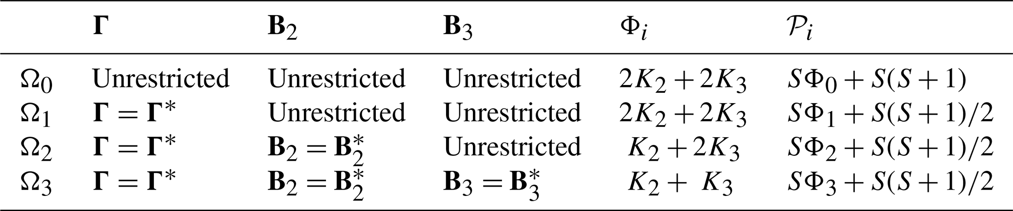
If H₀ is rejected, then we conclude that one or more of the VARX parameters differ, but which ones? A natural question is whether the difference in VARX models is due to differences in noise, differences in AR parameters, or differences in annual cycle parameters. This question is addressed by the following stepwise procedure: first test for differences in noise parameters, and if those are not significant, then test for differences in AR parameters, and if those are not significant, then test for differences in annual cycle parameters. This hierarchy of hypotheses is summarized in Table 1. Further details about the stepwise procedure, including the family-wise error rate and the reasons for choosing the particular order, are given in Sect. B7.

Table 1 Summary of hypotheses in the stepwise test procedure for VARX(p) models. Parameters Φ_i and 𝒫_i in the last two columns indicate the number of predictors and the number of estimated parameters under Hypothesis Ω_i, respectively.

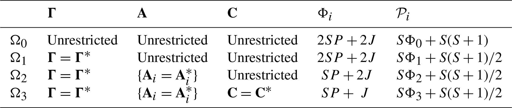
The statistic for testing Ω_i versus Ω_i+1 is called sub-deviance $D_{{\mathrm{\Omega }}_{i:i+\mathrm{1}}}$. Sub-deviance is small when the relevant parameter differences are small and large when the parameter differences are large. The associated significance thresholds are computed using a Monte Carlo technique (see Sect. B6). For our data, these thresholds are consistent with asymptotic theory, which indicates that, if Ω_i+1 is true, then asymptotically $D_{{\mathrm{\Omega }}_{i:i+\mathrm{1}}}$ is chi-squared distributed with ${\mathcal{P}}_i-{\mathcal{P}}_{i+\mathrm{1}}$ degrees of freedom, which we denote as

$$\begin{array}{}\text{(4)}& D_{{\mathrm{\Omega }}_{i:i+\mathrm{1}}}\sim {\mathit{\chi }}_{{\mathcal{P}}_i-{\mathcal{P}}_{i+\mathrm{1}}}^{\mathrm{2}},\end{array}$$

where 𝒫_i is the number of parameters estimated under Ω_i and specified in Table 1. The stepwise procedure halts at the first significant sub-deviance.

The deviance for testing the equality of all VARX parameters is the sum of the sub-deviances:

$$\begin{array}{}\text{(5)}& \begin{array}{ccccccc}{D}_{{\mathrm{\Omega }}_{\mathrm{0}:\mathrm{3}}}& =& D_{{\mathrm{\Omega }}_{\mathrm{0}:\mathrm{1}}}& +& D_{{\mathrm{\Omega }}_{\mathrm{1}:\mathrm{2}}}& +& D_{{\mathrm{\Omega }}_{\mathrm{2}:\mathrm{3}}}\\ \text{total}& & \text{noise}& & \text{AR}& & \text{annual cycle}.\end{array}\end{array}$$

Decomposition (5) is satisfied regardless of the status of the hypotheses in Table 1. Using these terms to quantify the fraction of deviance due to differences in noise, AR, or annual cycle parameters can be subtle. In particular, the largest term may not dictate significance. For instance, one term on the right-hand side might explain 90 % of the deviance and yet still be insignificant, whereas another term explains only 5 % of the deviance yet is significant. This issue should be kept in mind when quantifying the contribution of particular components of the VARX model to the total deviance.

The above procedure might attribute differences to a single part of the VARX model, but that part still involves many parameters, which hinders interpretation. To further isolate VARX model differences, we seek the linear combination of variables that maximizes the appropriate sub-deviance $D_{{\mathrm{\Omega }}_{i:i+\mathrm{1}}}$. A procedure called covariance discriminant analysis (CDA DelSole and Tippett, 2022a) can find this combination and leads to a decomposition that can be viewed as a generalization of principal component analysis. Specifically, CDA decomposes each $D_{{\mathrm{\Omega }}_{i:i+\mathrm{1}}}$ into S components such that the first maximizes $D_{{\mathrm{\Omega }}_{i:i+\mathrm{1}}}$, the second maximizes $D_{{\mathrm{\Omega }}_{i:i+\mathrm{1}}}$ subject to being uncorrelated with the first, and so on.

In the case of $D_{{\mathrm{\Omega }}_{\mathrm{0}:\mathrm{1}}}$, the interpretation of discriminant components is clear-cut: these components identify the spatial structures that exhibit the greatest discrepancies in whitened variances between the two data sets (see DelSole and Tippett, 2022a). For $D_{{\mathrm{\Omega }}_{\mathrm{1}:\mathrm{2}}}$ and $D_{{\mathrm{\Omega }}_{\mathrm{2}:\mathrm{3}}}$, however, the connection between these components and differences in VARX parameters is less apparent. In the Appendix, we clarify this connection by showing that sub-deviances can be written as an explicit function of differences in estimated regression parameters (see Sect. B8). To our knowledge, this result has not been derived previously. To describe this relation, let the matrix ${\widehat{\mathit{\delta }}}_{i+\mathrm{1}}$ denote the difference between estimated regression parameters relevant to comparing hypotheses Ω_i and Ω_i+1. For instance, to compare the Ω₁ and Ω₂ of a VARX(1) model, ${\widehat{\mathit{\delta }}}_{\mathrm{2}}^T={\widehat{\mathbf{A}}}_{\mathrm{1}}-{\widehat{\mathbf{A}}}_{\mathrm{1}}^{*}$. Then, the Appendix shows that the sub-deviance can be written as

$$D_{{\mathrm{\Omega }}_{i:i+\mathrm{1}}}=(\mathit{\nu }+{\mathit{\nu }}^{*})\log |\mathbf{I}+{\dot{\mathit{\delta }}}_{i+\mathrm{1}}^T{\dot{\mathit{\delta }}}_{i+\mathrm{1}}|\text{for }i\ge \mathrm{1},$$

where ${\dot{\mathit{\delta }}}_{i+\mathrm{1}}$ is a linear transformation of ${\widehat{\mathit{\delta }}}_{i+\mathrm{1}}$ (given explicitly in Eq. B34). A singular value decomposition (SVD) of ${\dot{\mathit{\delta }}}_{i+\mathrm{1}}$ then yields the desired decomposition of $D_{{\mathrm{\Omega }}_{i:i+\mathrm{1}}}$. From the SVD, one can either examine differences in regression parameters directly or examine their impact on the model. The latter is often more informative. For instance, when diagnosing differences in AR parameters, the decomposition can be expressed as

$$\begin{array}{}\text{(6)}& {\mathbf{P}}_X^T{\widehat{\mathit{\delta }}}_{\mathrm{2}}={\mathbf{SP}}_Y^T,\end{array}$$

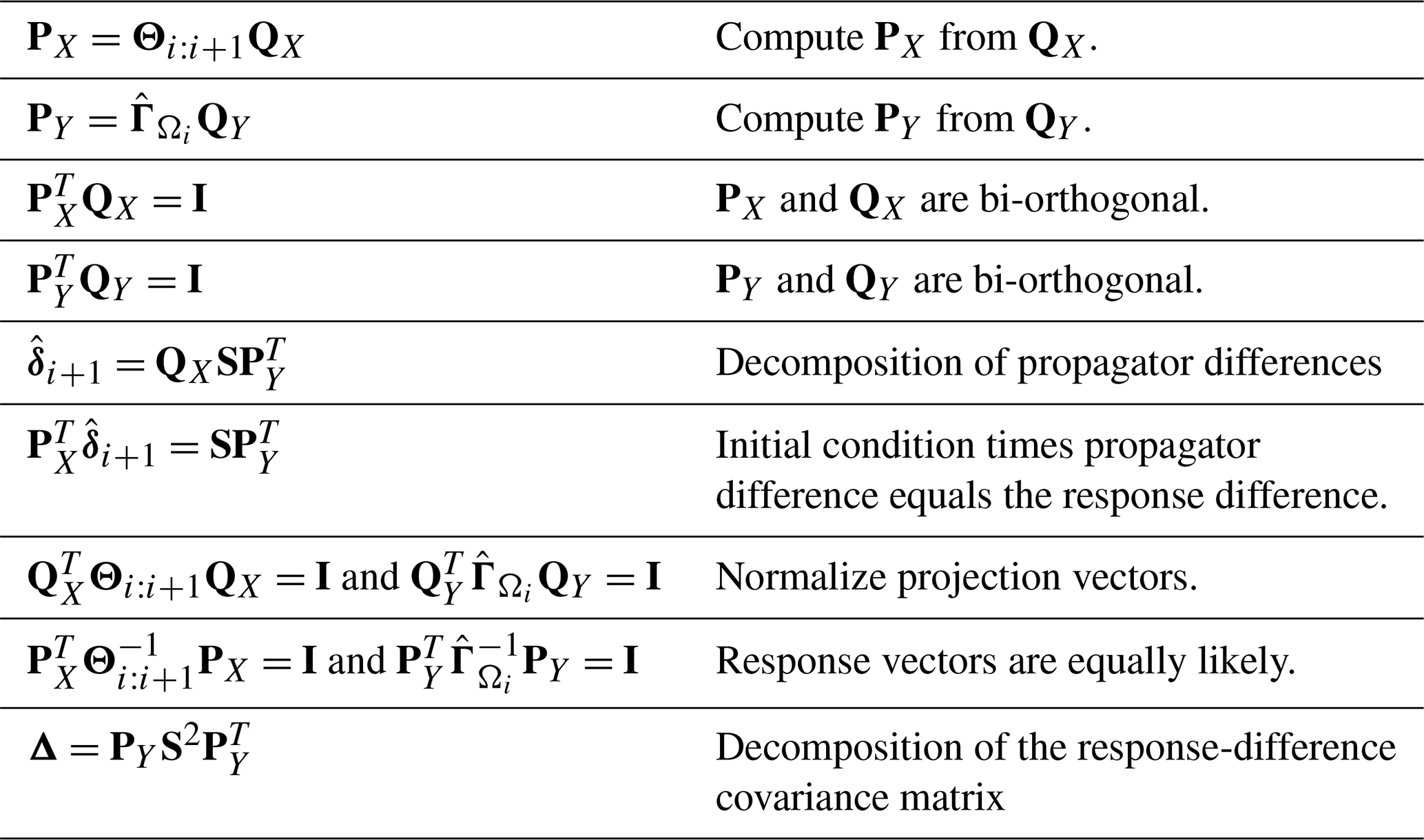
where ${\widehat{\mathit{\delta }}}_{\mathrm{2}}$ is the difference in AR parameters under Ω₁, S is a diagonal matrix, and the columns of P_X and P_Y define initial condition and response patterns, respectively (all the terms are defined precisely in Sect. B8). This decomposition has the following form: the initial condition (P_X) multiplied by the difference in AR parameters (${\widehat{\mathit{\delta }}}_{\mathrm{2}}$) equals the difference in the response (P_YS). This decomposition can be interpreted as finding the initial condition, among all equally likely initial states, that maximizes the disparity in one-step responses. This decomposition is similar to the “optimal initial condition” discussed in previous studies (e.g., Penland and Sardeshmukh, 1995; Alexander et al., 2008), except here the initial and final vectors are constrained by norms associated with the deviance measure.

To diagnose differences in annual cycle parameters, the above decomposition is not very meaningful because the predictor is a fixed function of time (e.g., sinusoidal functions of time) rather than a random vector. In this case, we simply propagate parameter differences into the time domain by multiplying by the associated predictors X, yielding a decomposition that is similar to principal component analysis in the form

$$\begin{array}{}\text{(7)}& \begin{array}{ccccc}\mathbf{X}{\widehat{\mathit{\delta }}}_{i+\mathrm{1}}& =& {\widehat{\widehat{\mathbf{Q}}}}_X& \mathbf{S}& {\mathbf{P}}_Y^T\\ \text{annual cycle}& & \text{time series}& \text{amplitude}& \text{spatial pattern}.\\ \text{differences}& \end{array}\end{array}$$

3 Application to North Atlantic variability

In this section, we apply the above method to compare the variability of monthly mean North Atlantic sea surface temperature (SST) between dynamical models and observations. We analyze the Atlantic basin over 0–60^∘ N, where the northern boundary was chosen to avoid regions of sea ice. For observations, we use version 5 of the Extended Reconstructed Sea Surface Temperature (ERSSTv5) of Huang et al. (2017). The earlier portion of this data set has sparse spatial coverage, so we only analyze the more recent 50-year period 1969–2018.

For model simulations, we use data from Phase 5 of the Coupled Model Intercomparison Project (CMIP5; Taylor et al., 2012). Specifically, we use pre-industrial control runs, which are simulations without year-to-year changes in external forcing like atmospheric composition or solar insolation. The associated initial condition is effectively random, and hence these simulations are independent, consistent with our assumptions in Eqs. (1) and (2). We select models only if their control runs are at least 500 years long. This criterion selects 36 models from the CMIP5 data set. We extract the last 50 years of each simulation. We examine the last two 25-year segments of each simulation and compare them with each other and with 25-year segments from observational data. While our test can accommodate time series of varying lengths, we found that a duration of 25 years is sufficient for detecting differences effectively.

In general, the above time series contain secular trends: observations contain a global warming signal and control runs contain model drift. These secular trends will be removed by regressing out a polynomial in time. It is important to remove the same-order polynomial from both observations and models; otherwise, a difference could arise simply as an artifact of processing the two time series differently. It is known that greenhouse gas concentrations rise exponentially over our analysis period (1969–2018), so if we were to remove only a linear trend and then find a difference, that difference could be attributed to quadratic growth in the observations that is missing from control runs. In general, leaving any kind of forced variability in time series leads to problems of interpretation since our VARX model does not account for secular forcing. On the other hand, over-removal of low-frequency internal variability poses a lesser issue. While the resulting analysis would not relate to low-frequency variability (since it was removed), the conclusions regarding higher-frequency variability would still retain their validity. Hence, it is generally preferable to err on the side of removing a higher-order polynomial than a lower-order one. For the results presented in the figures below, a second-order polynomial in time was removed over the period 1969–2018. However, removing third-, fourth-, or higher-order polynomials removes additional low-frequency variability from the time series but does not alter any of our main conclusions regarding significant differences between observations and CMIP5 models.

For the annual cycle term, we include five annual harmonics encompassing all harmonics up to the Nyquist frequency. This choice is motivated by the same reasoning as discussed above for secular trends, i.e., that it is preferable to include more harmonics rather than fewer. If we were to select an insufficient number of harmonics, then unaccounted-for periodic signals would be misattributed as internal variability in the VARX model, leading to erroneous conclusions. On the other hand, if an excessive number of harmonics is chosen, the VARX model may become overfitted, but this potential overfitting is accounted for in the sampling distribution. By definition, overfitting implies the inclusion of predictors with vanishing regression coefficients, but the sampling distribution is independent of the specific values of the regression coefficients and therefore encompasses cases where the coefficients are zero. The primary drawback of overfitting is a reduction in statistical power. However, in our specific application, low statistical power is not a concern: our method demonstrates high effectiveness in detecting differences when they truly exist. Therefore, the negative consequences associated with overfitting, such as diminished statistical power, are not a significant issue in this context.

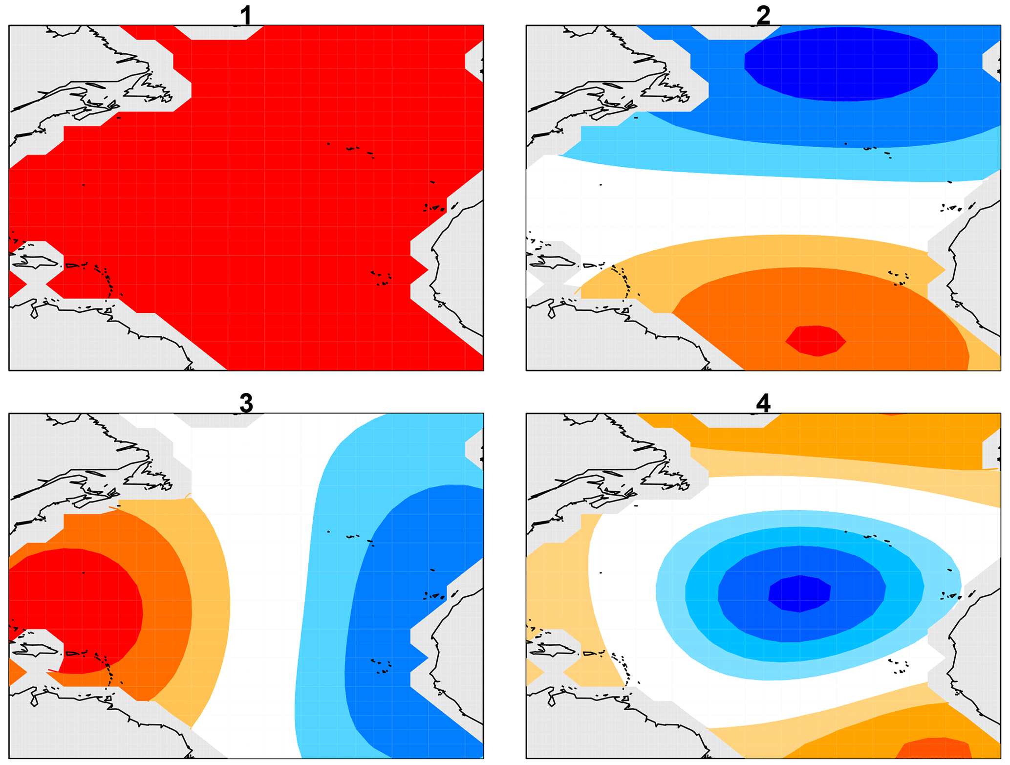
Figure 1 Laplacian eigenvectors 1, 2, 3, and 4 over the North Atlantic between the Equator and 60^∘ N, where dark red and dark blue indicate extreme positive and negative values, respectively.

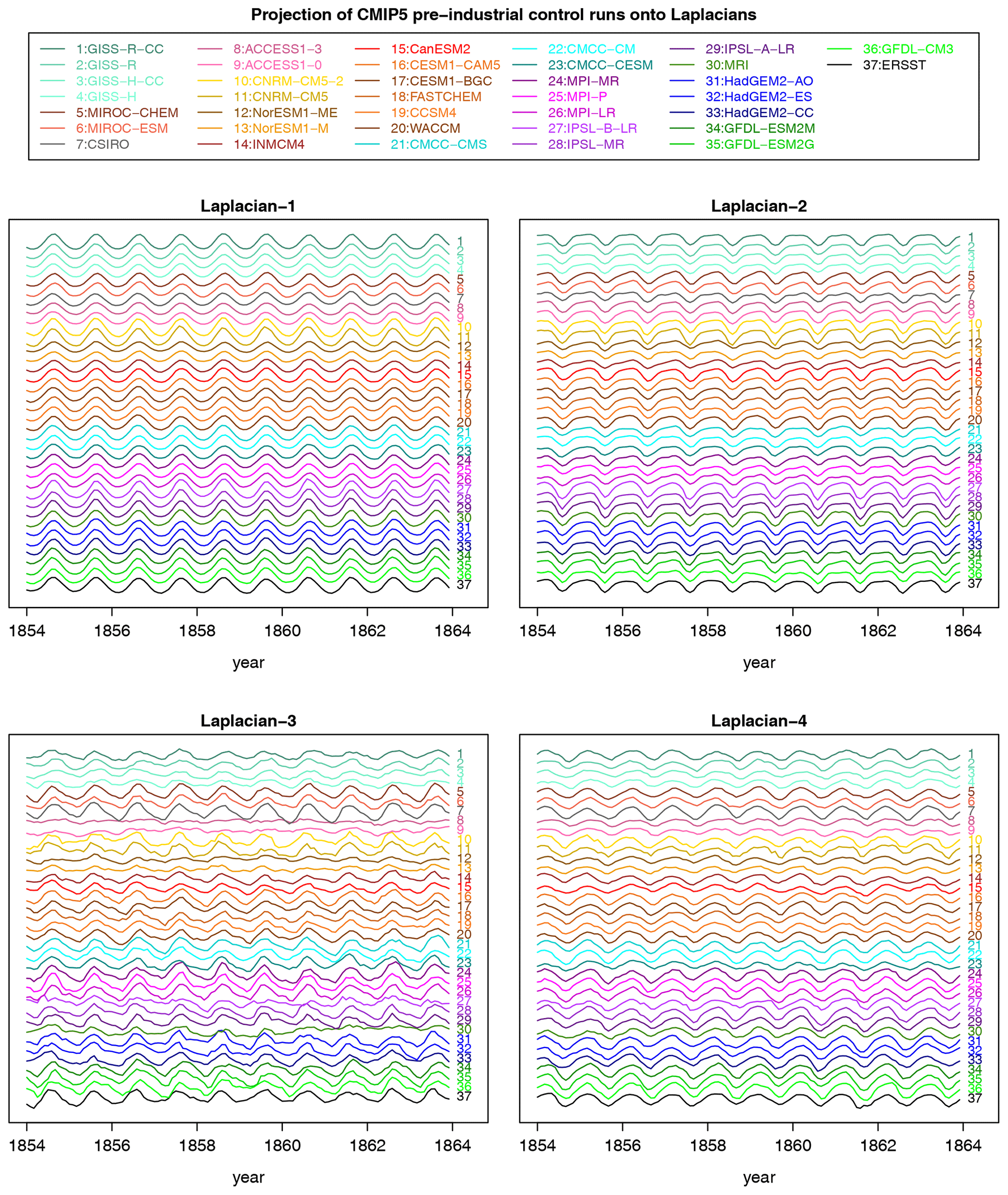
Figure 2 Monthly time series of Laplacians 1–4 in observations (black curve at the bottom labeled “37”) and in CMIP5 models over a 10-year period. Each time series is offset by the same constant. No re-scaling is performed. Each time series is computed by projecting data onto the appropriate Laplacian over the Atlantic domain. The year on the x axis corresponds to the observational data set ERSSTv5 but otherwise is a reference label for the pre-industrial control simulations.

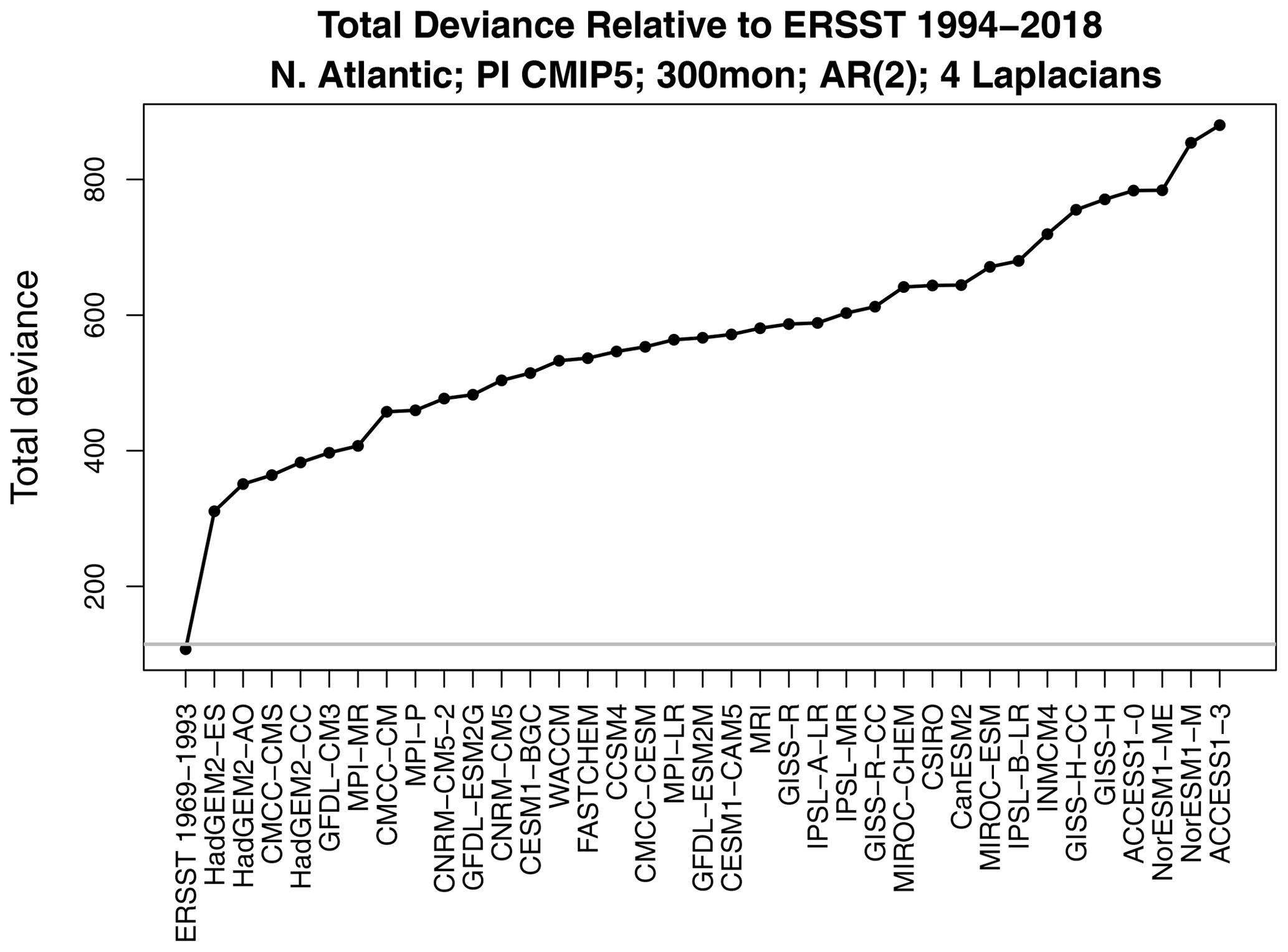
Figure 3 The total deviance between ERSSTv5 1994–2018 and each CMIP5 model. The horizontal gray line shows the 1 % significance threshold. Also shown is the deviance between ERSSTv5 for the two periods 1969–1993 and 1994–2018 (first x-tick mark on the left).

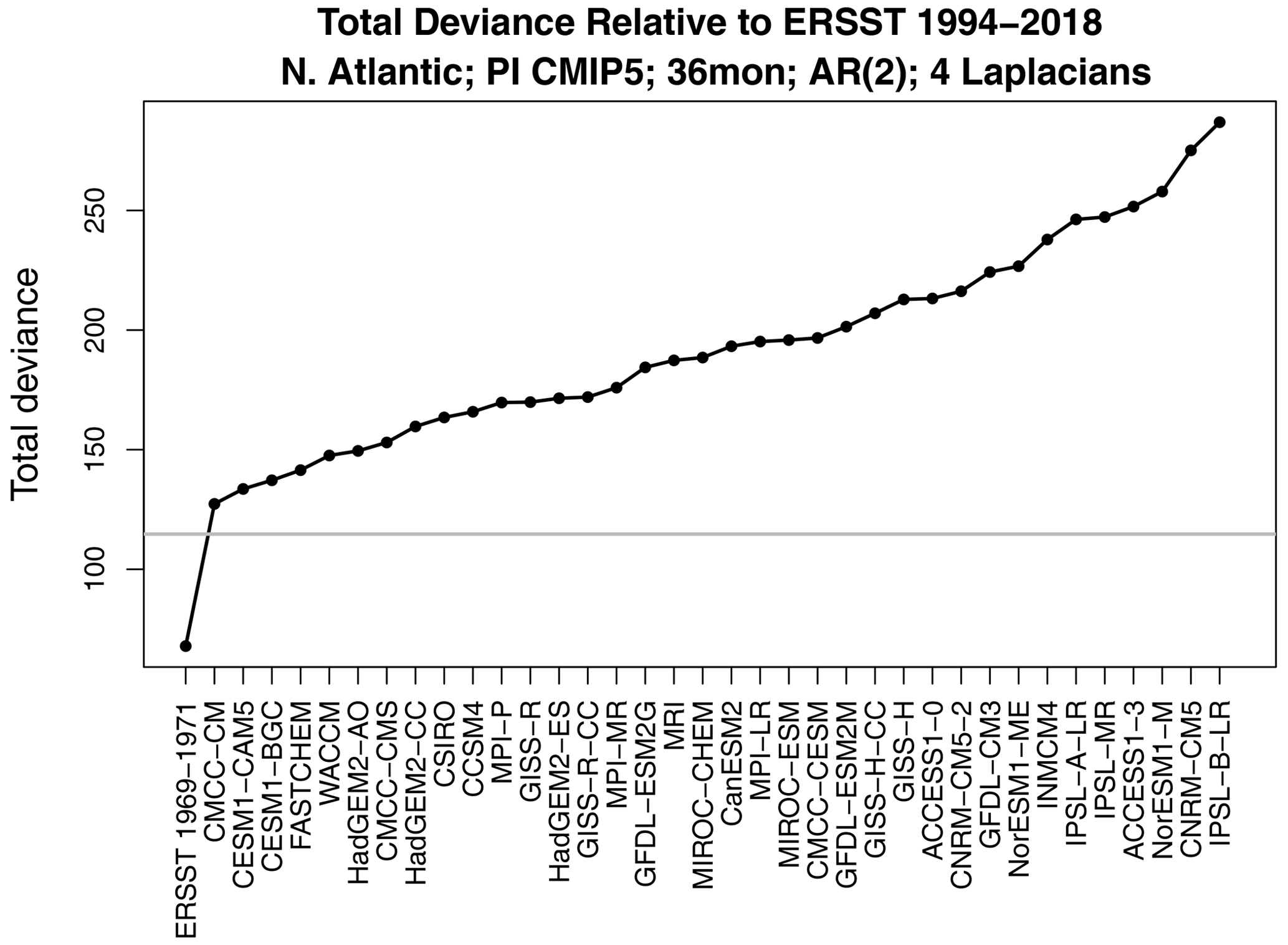
Figure 4 Same as Fig. 3 but using only 3 years of data from each CMIP5 model. Also shown is the deviance between ERSSTv5 for the two periods 1969–1971 (3 years) and 1994–2018 (first x-tick mark on the left).

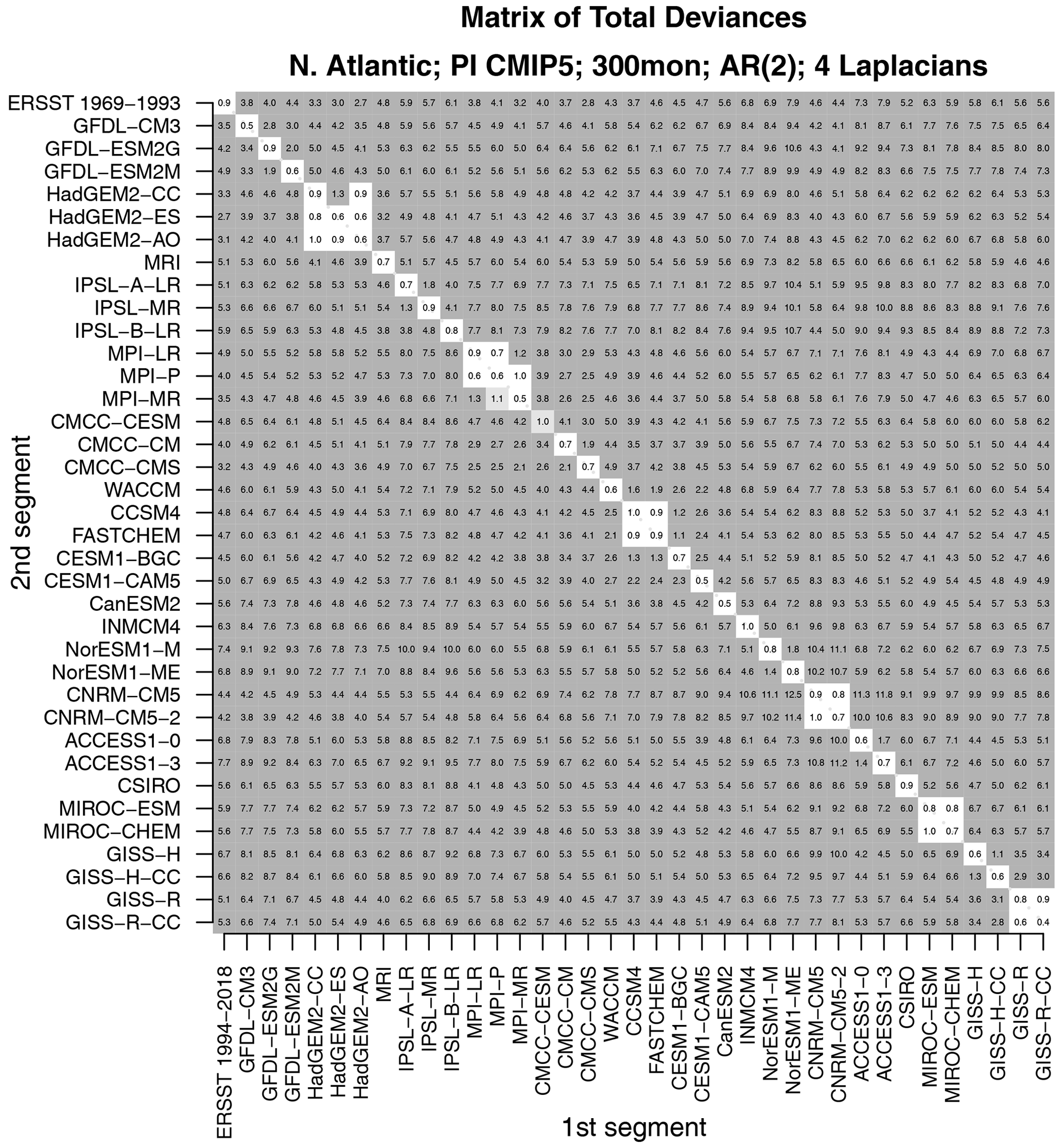
Figure 5 The total deviance between each 25-year segment from CMIP5 models and observations to an independent 25-year segment from CMIP5 models and observations. The deviance is normalized by the 1 % significance threshold. Values that are insignificant, significant at the 1 % level, and significant at the 0.2 % level are indicated by no shading, light gray shading, and dark gray shading, respectively.

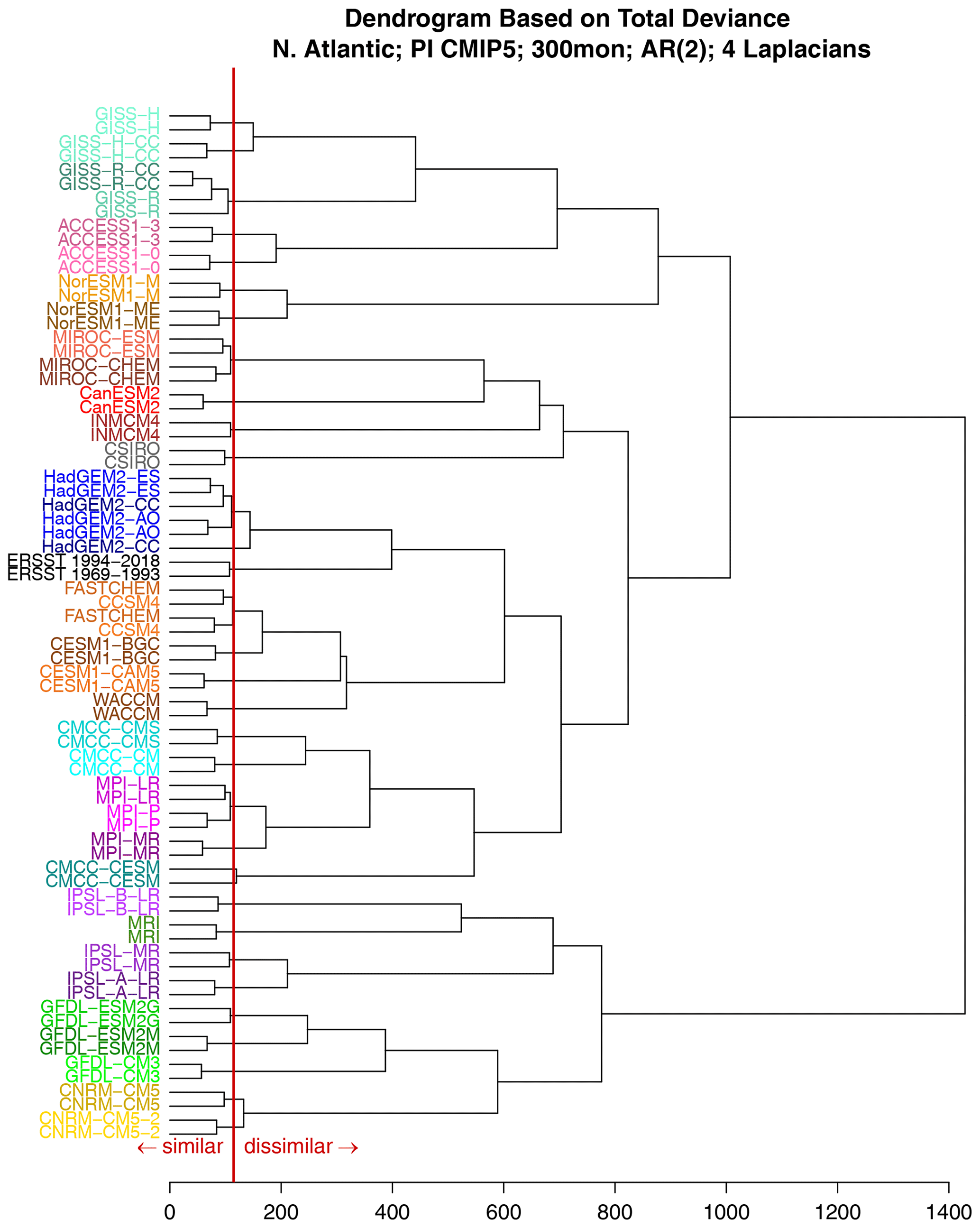
Figure 6 A dendrogram based on the total deviance of monthly mean North Atlantic SST. The x axis is the deviance. Larger deviance values imply stronger dissimilarities between the VARX models. All the time series are 25 years in length. Two separate 25-year segments from CMIP5 models and from observations (ERSSTv5) are included in the cluster analysis. The vertical red line shows the 1 % significance level.

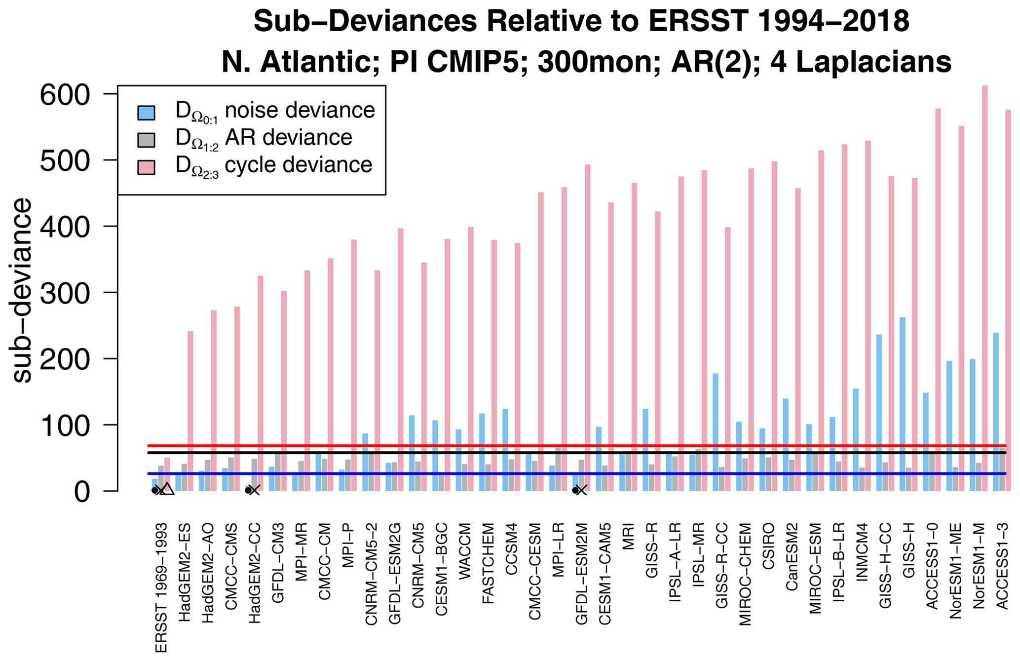
Figure 7 Decomposition of each deviance in Fig. 3 into differences in noise parameters (blue), differences in AR parameters (green), and differences in annual cycle parameters (red). The associated 1 % significance thresholds are indicated by the blue, green, and red horizontal lines, and sub-deviances that are insignificant according to the stepwise procedure are indicated by the dot, cross, and triangle, respectively.

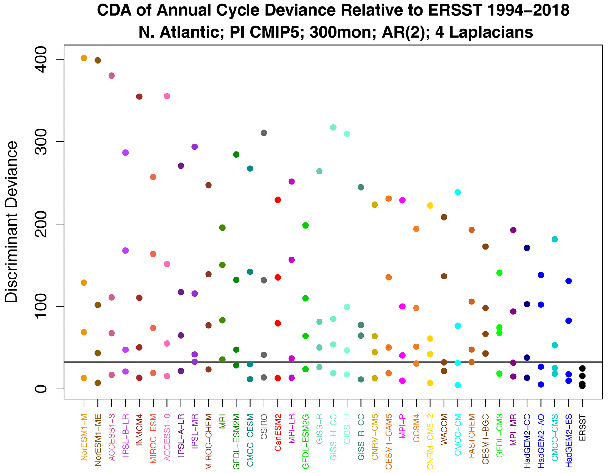
Figure 8 Decomposition of annual cycle deviance by discriminant analysis. The horizontal gray line is the 1 % significance threshold for the maximum deviance, computed as described at the end of Sect. B6.

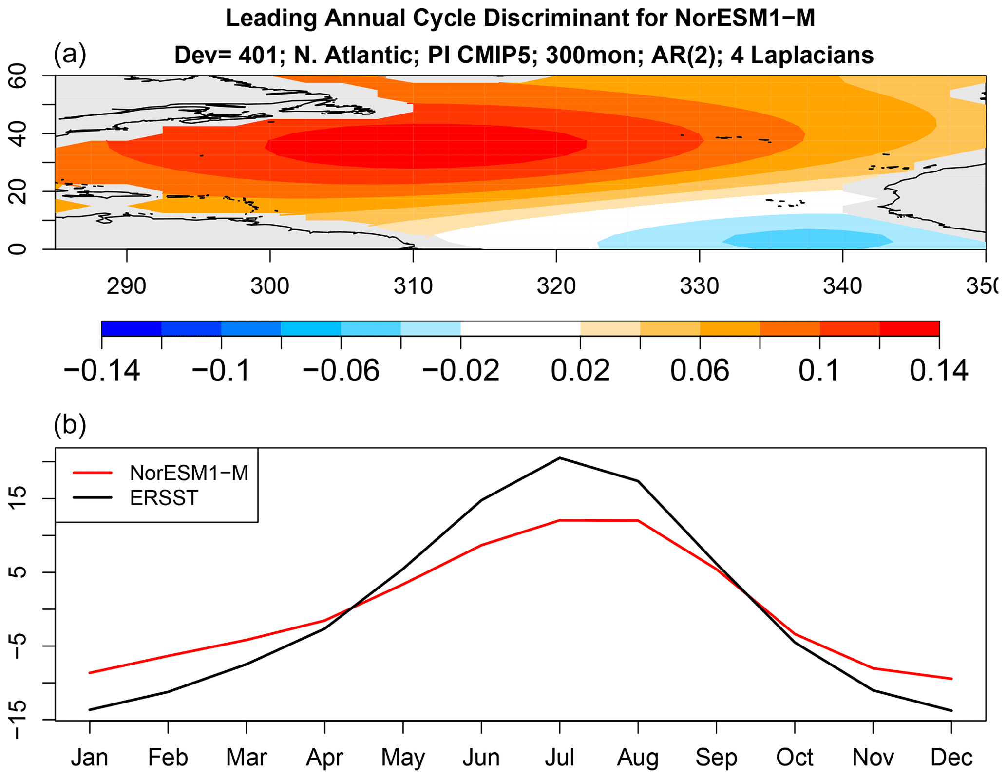
Figure 9 The spatial pattern (a) and time series (b) of the leading discriminant of the annual cycle deviance for NorESM1-M.

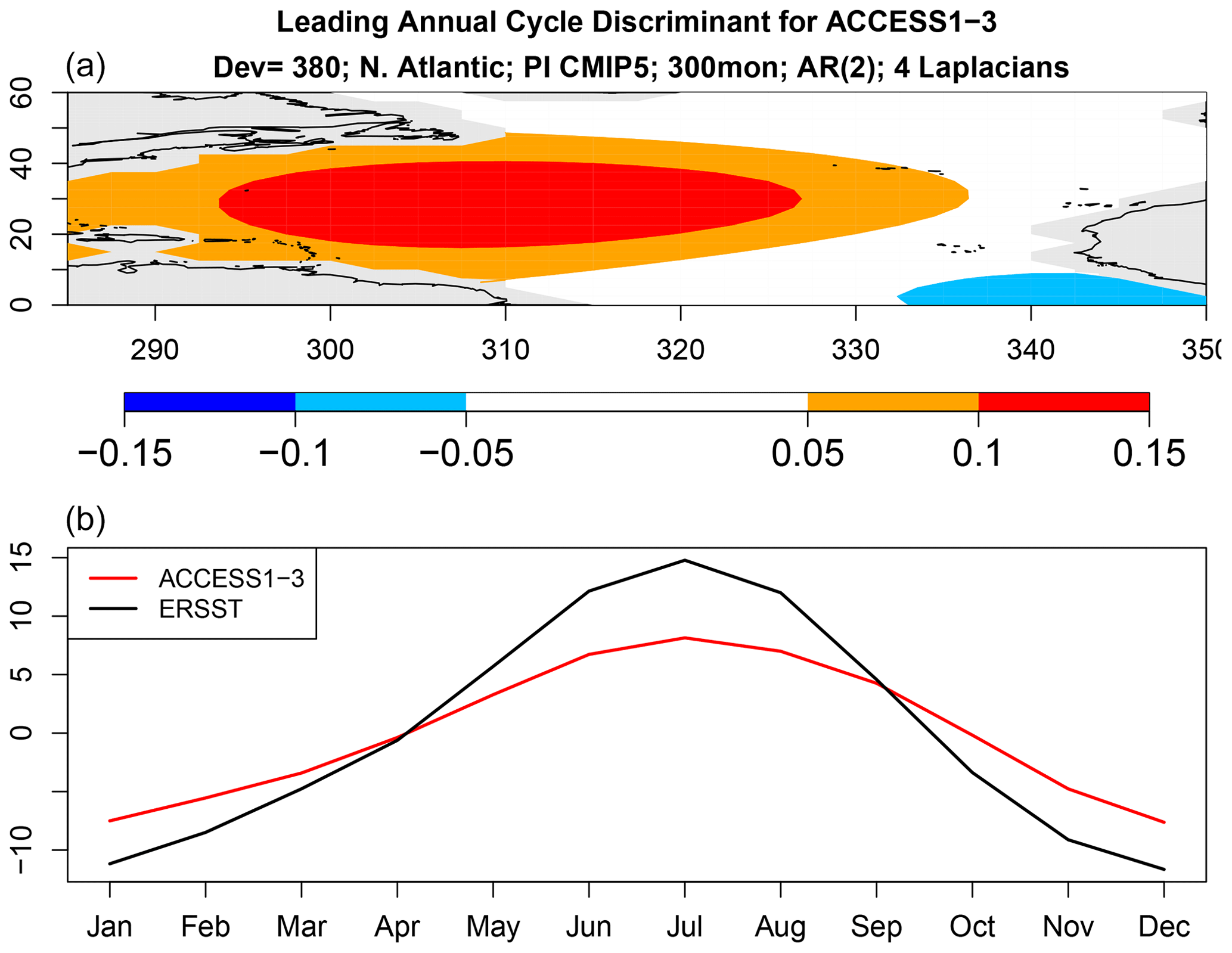
Figure 10 Same as Fig. 9 but for ACCESS1-3.

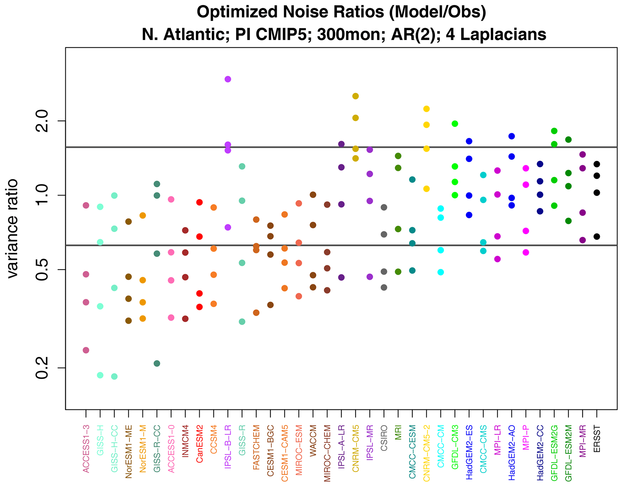
Figure 11 Variance ratios from discriminant analysis of noise variance, where the ratio is CMIP5 model noise variance over observation noise variance. The two horizontal gray lines indicate the upper and lower 0.5 % significance levels.

Figure 12 Same as Fig. 5 except for noise deviance.

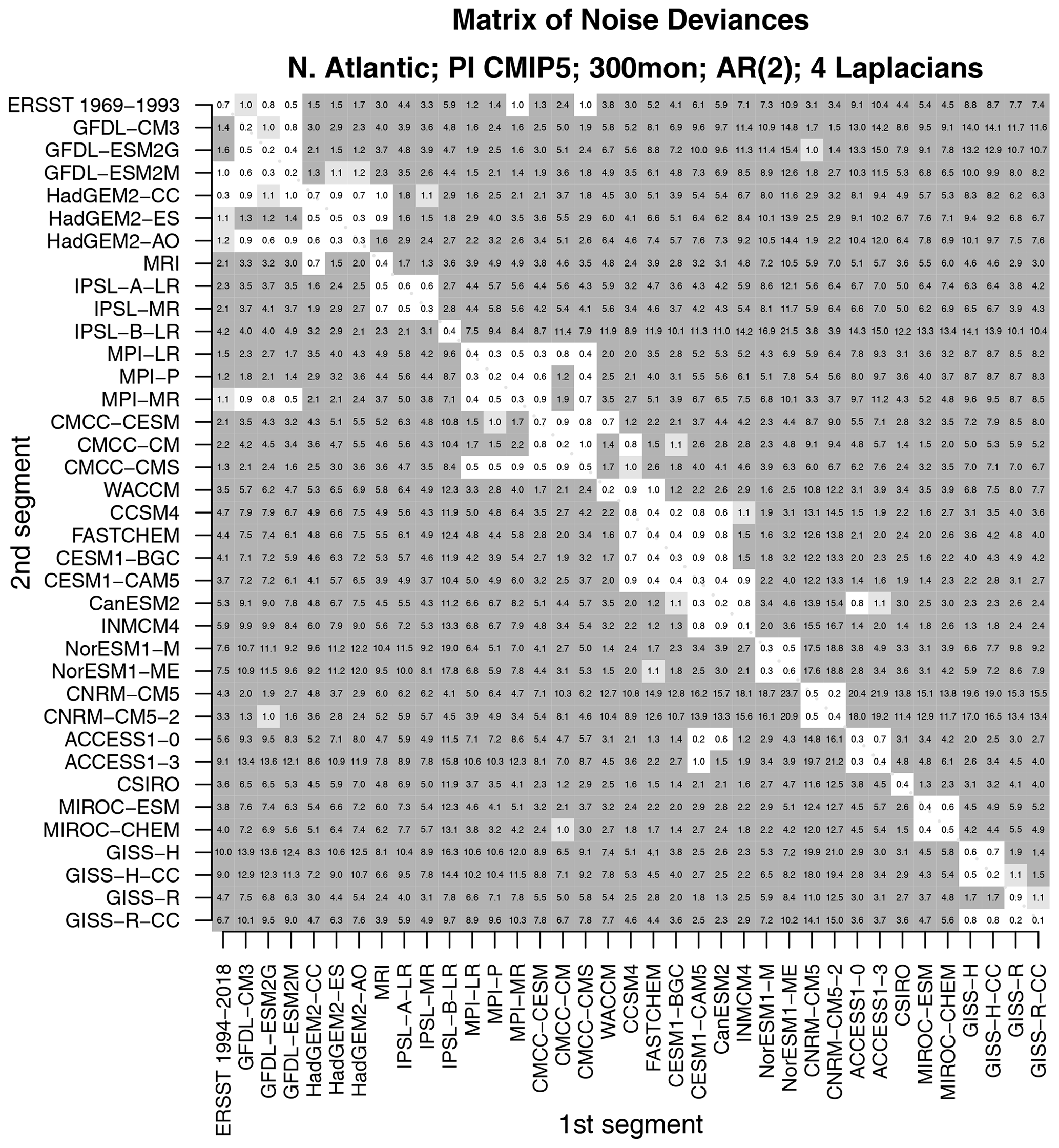
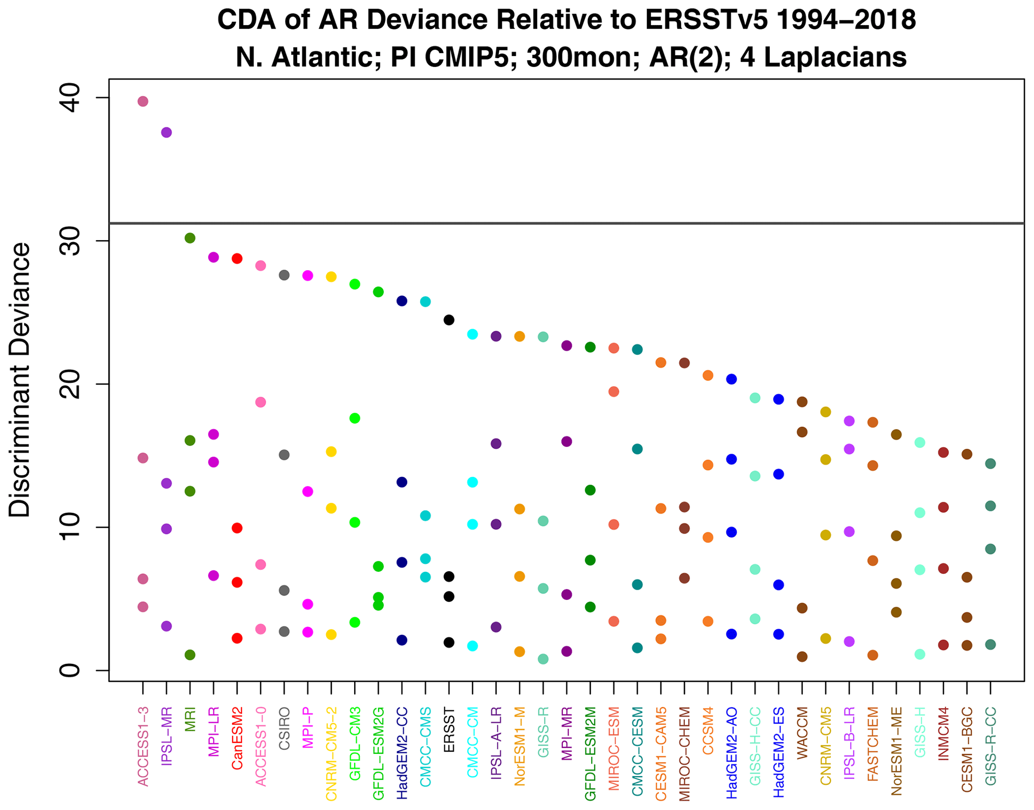
Figure 13 Decomposed AR deviance from discriminant analysis. The horizontal gray line indicates the 1 % significance threshold. Models on the x axis have been ordered by leading deviance.

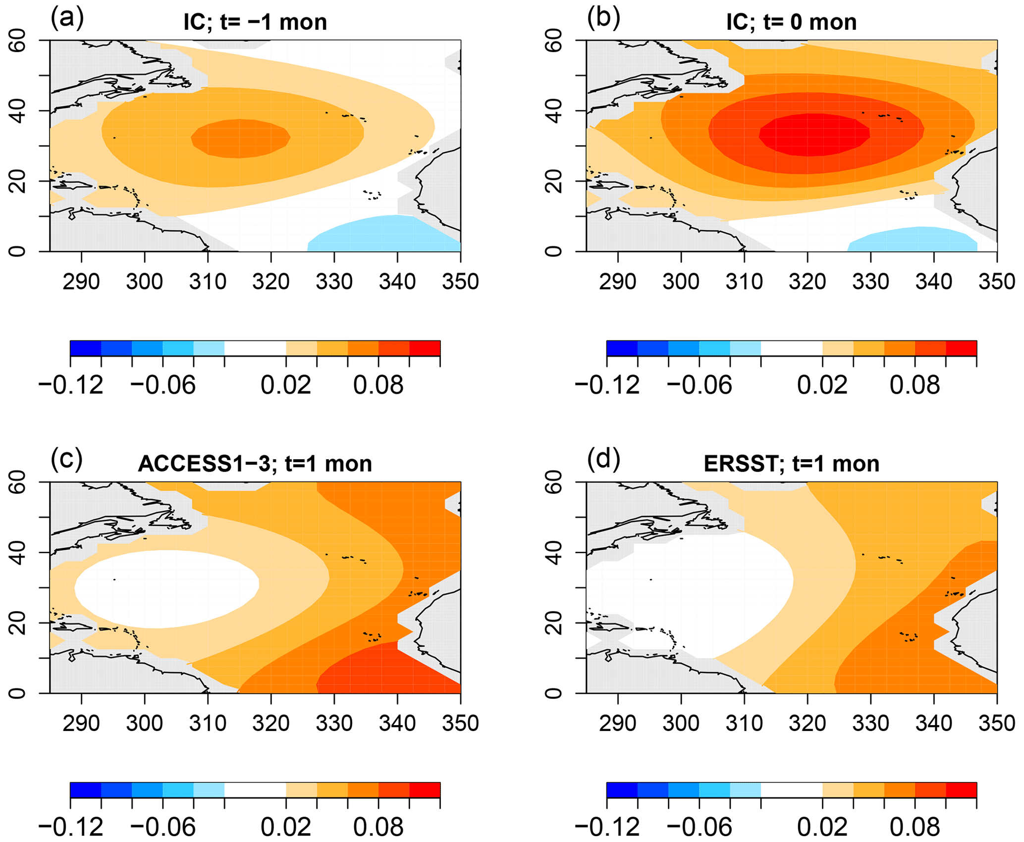
Figure 14 The optimal initial condition of VARX(2) models (a, b) that maximizes the difference in response between ACCESS1-3 and ERSSTv5 and the corresponding response in ACCESS1-3 (c) and ERSSTv5 (d).

As in many climate applications, the spatial dimension in our data set exceeds the time dimension, leading to an underdetermined estimation problem. Although several regularization approaches are available, many of these have no rigorous hypothesis test framework. Here, we regularize the problem by reducing the spatial dimension, which retains the regression model framework. The question arises as to which low-dimensional space should be selected. Our choice is guided by the fact that numerical solutions have less reliability with a decreasing spatial scale, with the least reliable results at the grid-point scale. These considerations suggest that models are most reliable on the largest spatial scales, and therefore a feature space should be chosen to emphasize large spatial scales. A common approach is to use empirical orthogonal functions (EOFs), but EOFs depend on data and therefore raise the question as to which data should be used to derive them. Also, there is no guarantee that the EOFs will be strictly large scale. Furthermore, because EOFs depend on data, their use leads to biases and random fluctuations that are not straightforward to take into account in the final statistical estimate. An attractive alternative basis set that avoids these issues and satisfies the above requirement contains the leading eigenvectors of Laplace's equation. These vectors form an orthogonal set of spatial patterns ordered by the decreasing spatial scale. Familiar examples of Laplacian eigenvectors include Fourier series and spherical harmonics. The algorithm of DelSole and Tippett (2015) was used to compute the Laplacian eigenvectors over the Atlantic domain. The first four eigenvectors are shown in Fig. 1. The first Laplacian eigenvector is spatially uniform, and therefore projecting data onto the first vector yields the spatial mean. The spatial mean of Atlantic SSTs after removal of human-caused variations is often called the Atlantic Multidecadal Variability (AMV) index. The second and third eigenvectors are dipoles measuring the north–south and east–west gradients across the basin. Subsequent vectors capture smaller-scale spatial structures. Compared to the usual choice of EOFs, Laplacian eigenvectors are particularly attractive because the first component is the AMV index, a natural climate index, and the set depends only on the domain geometry and hence is independent of data and independent of the model.

How many Laplacian eigenvectors should be chosen? In this study, our goal is to compare variability, not to make predictions. Accordingly, our primary concern is to ensure that the VARX(p) model is adequate. In practice, adequacy means confirming that the residuals of the estimated VARX(p) model are indistinguishable from white noise. The multivariate Ljung–Box test was performed on the residuals of the VARX(p) models to check for whiteness. For p=1, over half the VARX models exhibited significant non-whiteness at the 5 % level, regardless of the number of eigenvectors S. For p=2, only 16 % of the VARX models exhibited significant non-whiteness for S=4, with this percentage increasing for S>4. After a Bonferroni correction, significant non-whiteness was detected in only 1 out of 37 VARX models for S=4, suggesting that the VARX(2) model with S=4 and 5 annual harmonics is adequate.

For reference, 10-year segments of time series for the first four Laplacian eigenvectors are shown in Fig. 2. The strong periodicity seen in Laplacian-1 reflects the fact that 99 % of the variance is explained by the annual cycle. The strongest discrepancies between time series are seen in Laplacian-3, but this assessment is merely visual and subjective.

The total deviance between ERSSTv5 1994–2018 and each CMIP5 model is shown in Fig. 3. The corresponding 1 % significance threshold computed from Eq. (4) is indicated by the horizontal gray line. The first x-tick mark shows the deviance between ERSSTv5 for the two periods 1969–1993 and 1994–2018, which falls below the gray line, indicating no significant difference in stochastic processes between the two observational periods. In contrast, the deviance between observations and each CMIP5 model lies well above the significance threshold, indicating strong differences between stochastic processes. The same conclusion is reached when the reference period is switched from 1994–2018 to 1969–1993 (not shown).

The above examples are based on using 25 years of data for both climate models and observations. Adding more data merely makes the differences detected here even more significant. An interesting question is whether differences can be detected using shorter samples from climate models. Recomputing deviances using only 3 years of data (but still using 25 years of observational data) yields the results shown in Fig. 4. Remarkably, differences can still be detected, as indicated by the fact that all the deviances lie above the significance threshold. The same conclusion holds if we swap these numbers, i.e., use only 3 years of observations and 25 years of model data (not shown).

Two questions arise naturally here. First, do CMIP5 models differ from observations in a common way? This question can be addressed by comparing one model to another – a small deviance would indicate that the two models are similar and therefore differ from observations in a common way. Second, would the test correctly indicate that two time series from the same CMIP5 model are stochastically similar? Intuitively, data generated by the same model ought to be stochastically similar. However, this outcome is not assured. For instance, CMIP5 models are nonlinear and high-dimensional. There is no guarantee that variability from such models can be captured by a low-dimensional linear model. Also, our test assumes that sample sizes are sufficiently large to invoke a linear regression framework for testing hypotheses. Twenty-five years of data might not satisfy this requirement. These latter questions can be addressed by confirming that independent segments from the same CMIP5 model are stochastically indistinguishable. Both questions can be addressed by comparing one 25-year segment with a separate 25-year segment for all possible pairs of CMIP5 models and observations. The result of comparing all possible pairs is summarized in the matrix shown in Fig. 5.

As can be seen, values along the diagonal of this matrix are insignificant. Diagonal elements correspond to comparing time series from the same model or from the same observational data set. Thus, this test indicates that time series from the same source are stochastically indistinguishable, confirming that the test performs as expected. Additional insignificant deviances are found in diagonal blocks. For instance, the 2×2 block in the upper-left corner indicates that the two CNRM models are stochastically indistinguishable. The next blocks include the HadGEM2, MPI, NCAR, MIROC, and GISS models. In other words, models from the same center can be stochastically indistinguishable. Other than those cases, all other model–model deviances are significant. In short, models differ not only from observations, but also from each other, unless they come from the same center.

Although all the models are different, some models are more similar to each other than to others. To identify clusters, we compute a dendrogram from these deviances. The dendrogram is computed in the following way. First, each element is assigned to its own cluster. Next, the pair with the smallest deviance is clustered together using a “leaf” whose edge aligns with the deviance indicated on the x axis. Next, the pairs with the next smallest deviance are clustered together in the same way. Clusters themselves are joined to other elements or clusters using the complete-linkage rule, whereby the length of the leaf equals the maximum deviance among all pairs of members of the cluster. Each new cluster creates a new leaf further to the left corresponding to larger deviances. The resulting dendrogram is shown in Fig. 6.

Remarkably, the majority of model names on the left-hand side of the dendrogram are grouped into consecutive pairs, indicating a consistent pairing of time series originating from the same source. This suggests that each CMIP5 model simulation possesses a distinct “fingerprint” that can be quantified using the deviance measure. However, there are a few exceptions to this pattern, i.e., HadGEM2-CC, FASTCHEM, and CCSM4. These exceptions are paired with other models from the same modeling center, supporting the earlier conclusion that models from the same center may exhibit similarities that make them indistinguishable. Consequently, CMIP5 models from the same modeling center tend to share comparable fingerprints.

Which models are closest to the observations? According to the dendrogram, after clustering the observational time series together, they are subsequently grouped with HadGEM2 models and then with NCAR models (CESM, CCSM, and FASTCHEM). Importantly, the leaves connecting to observations surpass the significance threshold, consistent with the findings shown in Fig. 4. This implies that the HadGEM2 and NCAR models are the closest to the observations, although they still clearly differ from observations.

A natural question is whether the difference in VARX models is due to differences in noise parameters, AR parameters, or annual cycle parameters. This question can be addressed by computing the decomposition in Eq. (5). The results are shown in Fig. 7. We see immediately that the largest source of deviance is the annual cycle. In fact, if the annual cycle deviance were computed for all possible pairs, virtually the same structure as in Fig. 5 would emerge (not shown). This confirms that the annual cycle of any CMIP5 model differs not only from observations, but also from other models from different modeling centers. In other words, the annual cycle is also an effective fingerprint.

The above results show that the annual cycle in each CMIP5 model differs from observations and from other CMIP5 models, but they do not tell us how they differ. We can anticipate from Fig. 5 that there is no common difference, so any description of model error will be model-dependent. Nevertheless, even for a single model, isolating key differences is difficult because the annual cycle lies in a high-dimensional space. One could study plots of annual cycle differences, but eye-catching features may not be the features that contribute most to annual cycle deviance. This is where covariance discriminant analysis proves useful. Discriminant analysis decomposes sub-deviance into uncorrelated components ordered such that the first explains the most sub-deviance, the second explains the most sub-deviance subject to being uncorrelated with the first, and so on. If a few components explain all the sub-deviance, then discriminant analysis will find them. The result of applying discriminant analysis to decompose annual cycle deviance is shown in Fig. 8. Since the VARX model is based on four Laplacian eigenvectors, discriminant analysis decomposes sub-deviance into four components per model. The leading discriminant deviance is significant for all the CMIP5 models. In some models, the leading discriminant deviance exceeds the second by a factor of 3 or more (e.g., NorESM1 models and ACCESS1-3). The associated time series and pattern from decomposition (7) for NorESM1-M and ACCESS1-3 are shown in Figs. 9 and 10. Time series for observations and CMIP5 models separately are computed as described in Sect. B8 (see Eq. B41). The two figures suggest that the two CMIP models underestimate the winter and summer peaks in the Gulf Stream regions.

Sub-deviances that are insignificant according to the stepwise procedure are indicated by the dot, cross, and triangle for differences in noise, AR parameters, and annual cycle parameters, respectively. Only two models have insignificant differences in noise and AR parameters: HadGEM2-CC and GFDL-ESM2M. This means that the internal variability of these models is consistent with observations. To be fair, the noise and AR parameters of some other CMIP5 models are only marginally inconsistent with observations (e.g., the HadGEM2, MPI, and CMCC models). Also, if the observational reference is changed to the 1969–1993 period, then HadGEM2 is no longer consistent (not shown). In all the cases, the annual cycle of each CMIP5 model differs significantly from observations.

For some CMIP5 models, differences in noise parameters explain a large fraction of the total deviance. To assess whether these models exhibit common discrepancies in whitened variance, we calculate the noise deviance between all possible combinations of models and observations. The corresponding results are shown in Fig. 12. Relative to the total deviance shown in Fig. 5, noise deviance exhibits more cases of indistinguishable models. Still, many of these cases involve models originating from the same research center. Furthermore, each model remains distinctly different from the majority of other models, indicating that whitened variance alone can serve as a distinguishing feature or fingerprint. It is rather remarkable that, even after removing serial correlations, annual cycles, and trends, the remaining variability contains sufficient information to differentiate a model from most other models. Recall that the stepwise procedure begins by comparing whitened variances. This result shows that this first step already has large discriminative power even before differences in AR or annual cycle parameters are considered.

We applied covariance discriminant analysis to determine whether a few spatial structures can explain the noise deviance. The resulting discriminant ratios are shown in Fig. 11. Ratios are shown instead of deviances because ratios differentiate the direction of variance difference, whereas deviance is insensitive to direction as both smaller and larger whitened variances contribute to positive deviances. Each model yields four discriminant ratios since the VARX is based on four Laplacian eigenvectors. The strongest separations from one are those below one, indicating that CMIP5 models exhibit too little whitened variance compared to observations. Examination of the leading discriminant patterns for noise deviance across CMIP5 models (not shown) reveals no common bias structure, as one would anticipate from Fig. 12.

According to Fig. 7, the sub-deviance of AR parameter differences is relatively small. Nevertheless, for completeness, we show the associated discriminants. The discriminant deviances are shown in Fig. 13. As expected, most leading values are insignificant. The largest leading value occurs for ACCESS1-3. The associated AR parameter difference can be expressed as an initial value problem using Eq. (6). Note that this identifies the initial condition of a VARX(2) model, so the initial condition is defined by two SST patterns, one at the initial month and one at the antecedent month. The resulting patterns are shown in Fig. 14. The figure suggests that, for this initial condition, ACCESS1-3 responds with a stronger amplitude than observations, although the amplitude discrepancy is modest, consistent with the modest deviance level.

4 Conclusions

This paper presents a methodology for determining whether two vector time series originate from the same stochastic process. Such a procedure can be used to address various climate-related questions, including assessing the realism of climate simulations and quantifying changes in climate variability over time. The stochastic process under consideration is assumed to be a vector autoregressive model with exogenous variables, referred to as VARX. In this study, the exogenous variable represents annual cycles in the mean. However, in other applications, it could capture nonstationary signals such as diurnal cycles, secular changes due to solar variability, volcanic eruptions, or human-induced climate change. This paper derives a likelihood ratio test for determining the equality of VARX parameters. Additionally, an associated stepwise procedure is developed to determine the equality of noise parameters, autoregressive parameters, and annual cycle parameters. The resulting procedure is not limited to specific stochastic models employed in this study. Rather, the procedure is general and can be applied to a broader class of models, including non-periodic exogenous variables. Thus, these procedures provide a comprehensive framework for analyzing and comparing different aspects of climate time series.

Derivation of the above procedure follows an approach that is similar to the univariate case, but it is extended here to encompass multivariate applications. This extension necessitates the incorporation of bias corrections and the utilization of a Monte Carlo technique to estimate significance thresholds accurately. The Monte Carlo algorithm developed here is particularly efficient in that it uses eigenvalue methods to evaluate the ratio of determinants and avoids solving regression problems by sampling directly from the Wishart distribution. Discriminant techniques are employed to compress differences between VARX models into the minimal number of components, facilitating a more concise description. While similar techniques were introduced in previous parts of this paper series, this paper generalizes them to multivariate situations and to accommodate an arbitrary number of steps in the stepwise procedure. Consequently, the procedure and associated codes for this test supersede those discussed in earlier parts of the series, offering an improved and more comprehensive approach.

The above procedure was implemented to compare monthly mean North Atlantic sea surface temperatures between CMIP5 models and observational data, taking into account their respective annual cycles. The analysis focused on the variability projected onto the first four Laplacian eigenvectors over the North Atlantic basin, which highlight the largest spatial scales within the region. To ensure that the residuals exhibited properties akin to white noise, a VARX model of at least second order was required for most CMIP5 models. The test results indicated that not only do CMIP5 models differ stochastically from the observational data, but that they also display variations among themselves, except when models originate from the same modeling center. Differences among CMIP5 models are distinctive enough to serve as a fingerprint that differentiates a given model from any other model and from observational data.

The primary source of deviance from observations is disparities in annual cycles. To gain insight into the characteristics of these disparities, covariance discriminant analysis was employed to decompose deviance associated with annual cycles into uncorrelated components, ordered such that the first explains the largest portion of annual cycle deviance, the second explains the most deviance after the first has been removed, and so on. For certain CMIP5 models, the leading discriminant accounts for several times more annual cycle deviance than subsequent components. Specific examples of these leading discriminants were presented.

Although differences in annual cycles dominated the total deviance, differences in whitened variance were also significant across the majority of the models. Discriminant analysis revealed that most CMIP5 models underestimate whitened variance, with some models falling short by a factor of 5. A few models were found to overestimate whitened variance by a factor of 2 or more. The collective differences in whitened variances and covariances between Laplacian eigenvectors were sufficiently unique to serve as a secondary fingerprint. It is remarkable that such distinctive identifying information is encapsulated in time series even after removing serial correlations, annual cycles, and all other nonstationary signals such as trends.

Differences in autoregressive parameters accounted for only a minor portion of the overall deviance. Approximately two models displayed noise and AR parameters that aligned with observations, suggesting that their internal variability was realistically represented. However, all the models exhibited unrealistic annual cycles despite this positive characteristic.

The method discussed in this paper can analyze only relatively low-dimensional systems (for instance, the VARX model used to compare North Atlantic variability examined only four Laplacian eigenfunctions). It may be possible to combine some aspects of this approach with machine learning methods to greatly expand the number of variables that can be compared.

Appendix A: Likelihood ratio test

A standard method for testing hypotheses in VAR models is the maximum likelihood method (Brockwell and Davis, 1991; Box et al., 2008; Lütkepohl, 2005). The extension of this method to VARX models is straightforward. Specifically, the likelihood of Eq. (1) is

$$\begin{array}{}\text{(A1)}& \mathcal{L}={\left({\displaystyle \frac{L_P}{\left(\mathrm{2}\mathit{\pi }{)}^S\right|\mathbf{\Gamma }|}}\right)}^{(N^{\prime }-P)/\mathrm{2}}\exp \left[-\sum _{t=p+\mathrm{1}}^{N^{\prime }}{\widehat{\mathit{ϵ}}}_t^T{\mathbf{\Gamma }}^{-\mathrm{1}}{\widehat{\mathit{ϵ}}}_t/\mathrm{2}\right],\end{array}$$

where L_P represents terms that depend on the first p values of the process, and

$${\widehat{\mathit{ϵ}}}_t={\mathit{y}}_t-{\mathbf{A}}_{\mathrm{1}}{\mathit{y}}_{t-\mathrm{1}}-\mathrm{\dots }-{\mathbf{A}}_p{\mathit{y}}_{t-p}-\mathbf{C}{\mathit{f}}_t-\mathit{d}.$$

Similarly, the likelihood of Eq. (2) is

$$\begin{array}{}\text{(A2)}& {\mathcal{L}}^{*}={\left({\displaystyle \frac{L_P^{*}}{\left(\mathrm{2}\mathit{\pi }{)}^S\right|{\mathbf{\Gamma }}^{*}|}}\right)}^{(N^{\prime *}-P)/\mathrm{2}}\exp \left[-\sum _{t=p+\mathrm{1}}^{N^{\prime *}}{\widehat{\mathit{ϵ}}}_t^{*T}{\mathbf{\Gamma }}^{*-\mathrm{1}}{\widehat{\mathit{ϵ}}}_t^{*}/\mathrm{2}\right],\end{array}$$

where

$${\widehat{\mathit{ϵ}}}_t^{*}={\mathit{y}}_t^{*}-{\mathbf{A}}_{\mathrm{1}}^{*}{\mathit{y}}_{t-\mathrm{1}}^{*}-\mathrm{\dots }-{\mathbf{A}}_p^{*}{\mathit{y}}_{t-p}^{*}-{\mathbf{C}}^{*}{\mathit{f}}_t-{\mathit{d}}^{*}.$$

Since {y_t} and $\mathit{\left\{}{\mathit{y}}_t^{*}\mathit{\right\}}$ are independent, the likelihood of both models is the product of the two individual likelihoods:

$${\mathcal{L}}_{{\mathrm{\Omega }}_{\mathrm{0}}}=\mathcal{L}{\mathcal{L}}^{*}.$$

For the alternative hypotheses listed in Table 1, the likelihood is obtained by constraining the population parameters as indicated in Table 1. As an example, the likelihood under Ω₃ is

$$\begin{array}{rl}{\mathcal{L}}_{{\mathrm{\Omega }}_{\mathrm{3}}}& ={\left({\displaystyle \frac{L_P}{\left(\mathrm{2}\mathit{\pi }{)}^S\right|\mathbf{\Gamma }|}}\right)}^{(N^{\prime }-P)/\mathrm{2}}{\left({\displaystyle \frac{L_P^{*}}{\left(\mathrm{2}\mathit{\pi }{)}^S\right|\mathbf{\Gamma }|}}\right)}^{(N^{\prime *}-P)/\mathrm{2}}\\ & \exp \left[-\sum _{t=p+\mathrm{1}}^{N^{\prime }}{\widehat{\mathit{ϵ}}}_t^T{\mathbf{\Gamma }}^{-\mathrm{1}}{\widehat{\mathit{ϵ}}}_t/\mathrm{2}-\sum _{t=p+\mathrm{1}}^{N^{\prime }*}{\widehat{\mathit{ϵ}}}_t^{*T}{\mathbf{\Gamma }}^{-\mathrm{1}}{\widehat{\mathit{ϵ}}}_t^{*}/\mathrm{2}\right],\end{array}$$

where ${\widehat{\mathit{ϵ}}}_t$ and ${\widehat{\mathit{ϵ}}}_t^{*}$ take on the values

$$\begin{array}{ll}{\displaystyle }{\widehat{\mathit{ϵ}}}_t& {\displaystyle }={\mathit{y}}_t-{\mathbf{A}}_{\mathrm{1}}{\mathit{y}}_{t-\mathrm{1}}-\mathrm{\dots }-{\mathbf{A}}_p{\mathit{y}}_{t-p}-\mathbf{C}{\mathit{f}}_t-\mathit{d},\\ {\displaystyle }{\widehat{\mathit{ϵ}}}_t^{*}& {\displaystyle }={\mathit{y}}_t^{*}-{\mathbf{A}}_{\mathrm{1}}{\mathit{y}}_{t-\mathrm{1}}^{*}-\mathrm{\dots }-{\mathbf{A}}_p{\mathit{y}}_{t-p}^{*}-\mathbf{C}{\mathit{f}}_t-{\mathit{d}}^{*}.\end{array}$$

Maximum likelihood estimates are obtained by finding the parameters that maximize the likelihood in question. Unfortunately, this procedure is complicated by the terms L_p and $L_p^{*}$, which depend nonlinearly on the population parameters. However, for large N^′ and $N^{\prime *}$, the contribution of L_p and $L_p^{*}$ to the likelihood is small in comparison to other terms. A common approximation is to ignore L_p and $L_p^{*}$ when computing the maximum likelihood estimates, which is tantamount to maximizing the conditional likelihood and leads to the familiar least-squares estimates (Box et al., 2008, Sects. 7.1.2 and A7.4). Moreover, for asymptotically large sample sizes, the sampling distributions converge to those associated with linear regression theory. For example, see theorem 8.1.2 and Sect. 8.9 of Brockwell and Davis (1991) and Appendix A7.5 of Box et al. (2008) for the univariate case as well as Sect. 3.4 of Lütkepohl (2005) for the multivariate case. Accordingly, we assume that sample sizes are sufficiently large to justify asymptotic theory and therefore justify using linear regression theory to test hypotheses in VARX models. The problem of testing differences in VARX models is then addressed by appropriately mapping the parameters of the VARX model to the parameters of the regression model. This mapping can be performed in the following way. First, define

$$\mathit{\{}{\mathit{y}}_t{\mathit{\}}}_L^U=\left(\begin{array}{c}{\mathit{y}}_L\\ {\mathit{y}}_{L+\mathrm{1}}\\ \mathrm{⋮}\\ {\mathit{y}}_U\end{array}\right),$$

where L and U denote the lower and upper limits of a time series, respectively, with L<U. Then, the N^′ samples from model (1) are related as

$$\begin{array}{}\text{(A3)}& \mathbf{Y}={\mathbf{X}}_{\mathrm{2}}{\mathbf{B}}_{\mathrm{2}}+{\mathbf{X}}_{\mathrm{3}}{\mathbf{B}}_{\mathrm{3}}+{\mathbf{X}}_{\mathrm{4}}{\mathbf{B}}_{\mathrm{4}}+\mathbf{E},\end{array}$$

where

$$\begin{array}{rl}\mathbf{Y}& =\mathit{\{}{\mathit{y}}_t^T{\mathit{\}}}_{p+\mathrm{1}}^{N^{\prime }},{\mathbf{X}}_{\mathrm{2}}=\left(\begin{array}{ccc}\mathit{\{}{\mathit{y}}_t^T{\mathit{\}}}_p^{N^{\prime }-\mathrm{1}}& \mathrm{\dots }& \mathit{\{}{\mathit{y}}_t^T{\mathit{\}}}_{\mathrm{1}}^{N^{\prime }-p}\end{array}\right),\\ {\mathbf{X}}_{\mathrm{3}}& =\mathit{\{}{\mathit{f}}_t^T{\mathit{\}}}_{p+\mathrm{1}}^{N^{\prime }},{\mathbf{X}}_{\mathrm{4}}=\mathit{\{}\mathrm{1}{\mathit{\}}}_{p+\mathrm{1}}^{N^{\prime }},\end{array}$$

and

$${\mathbf{B}}_{\mathrm{2}}={\left(\begin{array}{cccc}{\mathbf{A}}_{\mathrm{1}}& {\mathbf{A}}_{\mathrm{2}}& \mathrm{\dots }& {\mathbf{A}}_p\end{array}\right)}^T,{\mathbf{B}}_{\mathrm{3}}={\mathbf{C}}^T,\text{and}{\mathbf{B}}_{\mathrm{4}}={\mathit{d}}^T.$$

In the context of comparing annual cycles,

$${\mathbf{X}}_{\mathrm{3}}=\left(\begin{array}{ccccccc}{\stackrel{\mathrm{̃}}{\mathit{c}}}_{\mathrm{1}}& {\stackrel{\mathrm{̃}}{\mathit{s}}}_{\mathrm{1}}& {\stackrel{\mathrm{̃}}{\mathit{c}}}_{\mathrm{2}}& {\stackrel{\mathrm{̃}}{\mathit{s}}}_{\mathrm{2}}& \mathrm{\dots }& {\stackrel{\mathrm{̃}}{\mathit{c}}}_H& {\stackrel{\mathrm{̃}}{\mathit{s}}}_H\end{array}\right),$$

where

$$\begin{array}{ll}{\displaystyle }{\stackrel{\mathrm{̃}}{\mathit{c}}}_h& {\displaystyle }=\mathit{\left\{}\cos \right(\mathrm{2}\mathit{\pi }h/\mathrm{12}t){\mathit{\}}}_{p+\mathrm{1}}^{N\prime }\\ {\displaystyle }{\stackrel{\mathrm{̃}}{\mathit{s}}}_h& {\displaystyle }=\mathit{\left\{}\sin \right(\mathrm{2}\mathit{\pi }h/\mathrm{12}t){\mathit{\}}}_{p+\mathrm{1}}^{N\prime }.\end{array}$$

Similarly, in an obvious notation,

$$\begin{array}{}\text{(A4)}& {\mathbf{Y}}^{*}={\mathbf{X}}_{\mathrm{2}}^{*}{\mathbf{B}}_{\mathrm{2}}^{*}+{\mathbf{X}}_{\mathrm{3}}^{*}{\mathbf{B}}_{\mathrm{3}}^{*}+{\mathbf{X}}_{\mathrm{4}}^{*}{\mathbf{B}}_{\mathrm{4}}^{*}+{\mathbf{E}}^{*}.\end{array}$$

In this way, the problem of comparing VARX models (1) and (2) is re-parameterized as the problem of comparing Eqs. (A3) and (A4). In the next section, we describe the procedure for comparing Eqs. (A3) and (A4). For this description, it proves convenient to define

$$\begin{array}{}\text{(A5)}& N=N^{\prime }-p\text{and}{N}^{*}=N^{\prime *}-p.\end{array}$$

Appendix B: Multivariate test of the equality of regression models

B1 Regression model framework

Although our goal is to describe the procedure for comparing the regression models (A3) and (A4), it turns out to be more efficient to describe the procedure in the context of the more general problem of comparing the models:

$$\begin{array}{}\text{(B1)}& {\displaystyle }\mathbf{Y}& {\displaystyle }={\mathbf{X}}_{\mathrm{2}}{\mathbf{B}}_{\mathrm{2}}+{\mathbf{X}}_{\mathrm{3}}{\mathbf{B}}_{\mathrm{3}}+\mathrm{\dots }+{\mathbf{X}}_{\mathit{\kappa }}{\mathbf{B}}_{\mathit{\kappa }}+\mathbf{E},\text{(B2)}& {\displaystyle }{\mathbf{Y}}^{*}& {\displaystyle }={\mathbf{X}}_{\mathrm{2}}^{*}{\mathbf{B}}_{\mathrm{2}}^{*}+{\mathbf{X}}_{\mathrm{3}}^{*}{\mathbf{B}}_{\mathrm{3}}^{*}+\mathrm{\dots }+{\mathbf{X}}_{\mathit{\kappa }}^{*}{\mathbf{B}}_{\mathit{\kappa }}^{*}+{\mathbf{E}}^{*},\end{array}$$

where X_k and ${\mathbf{X}}_k^{*}$ are predictor matrices, each having linearly independent columns; B_k and ${\mathbf{B}}_k^{*}$ are regression coefficients; and E and E^* are independent random matrices whose rows are drawn from a multivariate normal distribution with zero mean and covariance matrices Γ and Γ^*, respectively. These terms have the following dimensions:

$$\begin{array}{cccc}\mathbf{Y}\in {\mathbb{R}}^{N\times S},& {\mathbf{X}}_k\in {\mathbb{R}}^{N\times K_k},& {\mathbf{B}}_k\in {\mathbb{R}}^{K_k\times S},& \mathbf{E}\in {\mathbb{R}}^{N\times S},\\ {\mathbf{Y}}^{*}\in {\mathbb{R}}^{N^{*}\times S},& {\mathbf{X}}_k^{*}\in {\mathbb{R}}^{N^{*}\times K_k},& {\mathbf{B}}_k^{*}\in {\mathbb{R}}^{K_k\times S},& {\mathbf{E}}^{*}\in {\mathbb{R}}^{N^{*}\times S},\end{array}$$

where $k=\mathrm{2},\mathrm{\dots },\mathit{\kappa }$, and N and N^* are defined in Eq. (A5). S is the number of variables (i.e., the dimension of y_t in Eq. 1). $K_{\mathrm{2}},K_{\mathrm{3}},\mathrm{\dots },K_{\mathit{\kappa }}$ are the number of predictors in ${\mathbf{X}}_{\mathrm{2}},{\mathbf{X}}_{\mathrm{3}},\mathrm{\dots },{\mathbf{X}}_{\mathit{\kappa }}$.

Samples from VARX(p) models (1) and (2) can be written in the regression model forms (B1) and (B2) as discussed in Appendix A. The partitioning of parameters in models (1) and (2) into the B_i matrices in Eqs. (B1) and (B2) is highly adaptable and allows for considerable flexibility. To test the hypotheses in Table 1, B₂ would be identified with the AR parameters $\mathit{\{}{\mathbf{A}}_{\mathrm{1}},\mathrm{\dots },{\mathbf{A}}_p\mathit{\}}$, B₃ would be identified with the exogenous parameters C, and B₄ would be identified with the intercept. It is a matter of choice whether to test the equality of B₄. In Sect. 3, equality of climatological means was not tested, and hence the equality of B₄ was not tested. Under this identification, K₂=pS, K₃=J, and K₄=1. The identification of starred variables follows the same pattern. The null hypothesis H₀ in Eq. (3) corresponds to the hypothesis that ${\mathbf{B}}_i={\mathbf{B}}_i^{*}$ for $i=\mathrm{1},\mathrm{\dots },\mathit{\kappa }-\mathrm{1}$ and $\mathbf{\Gamma }={\mathbf{\Gamma }}^{*}$.

B2 Stepwise testing procedure

If H₀ is rejected, then one or more of the equalities in Eq. (3) is false, but which ones? To address this question, we test hypotheses about subsets of parameters. The hypothesis $\mathbf{\Gamma }={\mathbf{\Gamma }}^{*}$ is tested first for reasons discussed in DelSole and Tippett (2022b). Then, hypotheses about other parameter subsets are tested. Seber (2015) describes an elegant procedure for testing hypotheses in a stepwise manner. This procedure was adopted in DelSole and Tippett (2022b) and will be generalized further in this Appendix to include multivariate models. The least restrictive hypothesis is denoted as Ω₀, and subsequent hypotheses ${\mathrm{\Omega }}_{\mathrm{1}},\mathrm{\dots },{\mathrm{\Omega }}_{\mathit{\kappa }}$ are nested as ${\mathrm{\Omega }}_{\mathit{\kappa }}\subset {\mathrm{\Omega }}_{\mathit{\kappa }-\mathrm{1}}\subset \mathrm{\dots }\subset {\mathrm{\Omega }}_{\mathrm{0}}$. The first few hypotheses are indicated in Table B1. Note that Hypothesis H₀ is not Ω₀. Also, model (B1) deliberately excludes X₁ and B₁, so that hypotheses ${\mathrm{\Omega }}_{\mathrm{2}},{\mathrm{\Omega }}_{\mathrm{3}},{\mathrm{\Omega }}_{\mathrm{4}}$ in Table B1 correspond to restricting B₂,B₃, and B₄, respectively. Had the subscripts of B started at one, the resulting subscripts on Ω and B would have differed by one, leading to an awkward notation.

Table B1 Summary of the first few hypotheses in the stepwise procedure. Parameters Φ_i and 𝒫_i in the last two columns indicate the number of predictors and the number of estimated parameters under Hypothesis Ω_i, respectively.

A key quantity in the stepwise procedure is the number of parameters estimated under the ith hypothesis, denoted as 𝒫_i. Table B1 summarizes the number of parameters 𝒫_i and the number of predictors Φ_i associated with each hypothesis. For instance, the population parameters in Eq. (B1) are ${\mathbf{B}}_{\mathrm{1}},\mathrm{\dots },{\mathbf{B}}_{\mathit{\kappa }},\mathbf{\Gamma }$. Each B_i contains K_i predictors and therefore SK_i parameters, and Γ contains $S(S+\mathrm{1})/\mathrm{2}$ independent parameters. Model (B2) contains the same number of parameters. Therefore, the total number of parameters estimated under Ω₀ is

$${\mathcal{P}}_{\mathrm{0}}=\sum _{h=\mathrm{2}}^{\mathit{\kappa }}\mathrm{2}S{K}_h+S(S+\mathrm{1}).$$

Under Ω₁, the population parameters are ${\mathbf{B}}_{\mathrm{1}},{\mathbf{B}}_{\mathrm{1}}^{*},\mathrm{\dots },{\mathbf{B}}_{\mathit{\kappa }},{\mathbf{B}}_{\mathit{\kappa }}^{*},\mathbf{\Gamma }$. In particular, there is only one noise covariance matrix, so

$${\mathcal{P}}_{\mathrm{1}}=\sum _{h=\mathrm{2}}^{\mathit{\kappa }}\mathrm{2}S{K}_h+S(S+\mathrm{1})/\mathrm{2}.$$

As the stepwise procedure marches from Ω_i to Ω_i+1, there are K_i+1 fewer predictors estimated. Thus, in general, the number of parameters estimated under Ω_i for $\mathrm{1}\le i\le \mathit{\kappa }$ is

$${\mathcal{P}}_i=\sum _{h=\mathrm{2}}^{\mathit{\kappa }}(\mathrm{1}+H(h-i\left)\right)S{K}_h+S(S+\mathrm{1})/\mathrm{2},$$

where H(x) is a step function, which equals 0 when x≤0 and equals 1 when x>0 (note that H(0)=0).

B3 Equality of noise covariance matrices

The initial hypothesis in the stepwise test procedure is Ω₁, which asserts the equality of noise covariance matrices. This test shares similarities with the conventional test for equality of covariance matrices (e.g., Anderson, 1984, Chap. 10). However, certain adjustments are made, as discussed in more detail below, including an adjustment in the degrees of freedom to accommodate regression and the implementation of a bias correction. We start by expressing Eq. (B1) in the following form:

$$\begin{array}{}\text{(B3)}& \mathbb{Y}=\mathbb{X}\mathbb{B}+\mathbb{E},\end{array}$$

where

$$\mathbb{Y}=\mathbf{Y},\mathbb{X}=\left[\begin{array}{ccc}{\mathbf{X}}_{\mathrm{1}}& \mathrm{\dots }& {\mathbf{X}}_{\mathit{\kappa }}\end{array}\right],\text{and}\mathbb{B}=\left[\begin{array}{c}{\mathbf{B}}_{\mathrm{1}}\\ \mathrm{⋮}\\ {\mathbf{B}}_{\mathit{\kappa }}\end{array}\right].$$

By standard theorems, the maximum likelihood estimate of 𝔹 is

$$\widehat{\mathbb{B}}={\left({\mathbb{X}}^T\mathbb{X}\right)}^{-\mathrm{1}}{\mathbb{X}}^T\mathbb{Y},$$

the maximum likelihood estimate of Γ is

$$\begin{array}{}\text{(B4)}& \stackrel{\mathrm{‾}}{\mathbf{\Gamma }}={\left(\mathbb{Y}-\mathbb{X}\widehat{\mathbb{B}}\right)}^T\left(\mathbb{Y}-\mathbb{X}\widehat{\mathbb{B}}\right)/N,\end{array}$$

and the distribution of $\stackrel{\mathrm{‾}}{\mathbf{\Gamma }}$ is

$$\begin{array}{}\text{(B5)}& N\stackrel{\mathrm{‾}}{\mathbf{\Gamma }}\sim {\mathcal{W}}_S\left(\mathit{\nu },\mathbf{\Gamma }\right),\end{array}$$

where the right-hand side denotes an S-dimensional Wishart distribution with ν degrees of freedom and covariance matrix Γ. The degrees of freedom for model (B1) is

$$\begin{array}{}\text{(B6)}& \mathit{\nu }=N-K_{\mathrm{1}}-K_{\mathrm{2}}-\mathrm{\dots }-K_{\mathit{\kappa }}.\end{array}$$

Analogous results hold for model (B2), where the associated estimates are distinguished by asterisks. In particular, the estimated noise covariance matrix has distribution

$$\begin{array}{}\text{(B7)}& N^{*}{\stackrel{\mathrm{‾}}{\mathbf{\Gamma }}}^{*}\sim {\mathcal{W}}_S\left({\mathit{\nu }}^{*},{\mathbf{\Gamma }}^{*}\right),\end{array}$$

where

$$\begin{array}{}\text{(B8)}& {\mathit{\nu }}^{*}=N^{*}-K_{\mathrm{1}}-K_{\mathrm{2}}-\mathrm{\dots }-K_{\mathit{\kappa }}.\end{array}$$

The likelihood ratio for testing Ω₁ versus Ω₀ is

$${\displaystyle \frac{L_{{\mathrm{\Omega }}_{\mathrm{1}}}}{L_{{\mathrm{\Omega }}_{\mathrm{0}}}}}={\left({\displaystyle \frac{\left|\stackrel{\mathrm{‾}}{\mathbf{\Gamma }}{|}^N\right|{\stackrel{\mathrm{‾}}{\mathbf{\Gamma }}}^{*}{|}^{N^{*}}}{|{\stackrel{\mathrm{‾}}{\mathbf{\Gamma }}}_{{\mathrm{\Omega }}_{\mathrm{1}}}{|}^{N+N^{*}}}}\right)}^{\mathrm{1}/\mathrm{2}},$$

where $|\cdot |$ denotes the determinant of a matrix and ${\stackrel{\mathrm{‾}}{\mathbf{\Gamma }}}_{{\mathrm{\Omega }}_{\mathrm{1}}}$ is the maximum likelihood estimate of Γ under Ω₁, i.e.,

$$\begin{array}{}\text{(B9)}& {\stackrel{\mathrm{‾}}{\mathbf{\Gamma }}}_{{\mathrm{\Omega }}_{\mathrm{1}}}={\displaystyle \frac{N\stackrel{\mathrm{‾}}{\mathbf{\Gamma }}+N^{*}{\stackrel{\mathrm{‾}}{\mathbf{\Gamma }}}^{*}}{N+N^{*}}}.\end{array}$$

The corresponding sub-deviance statistic is therefore

$$D_{{\mathrm{\Omega }}_{\mathrm{0}:\mathrm{1}}}^{\prime }=(N+N^{*})\log \left|{\stackrel{\mathrm{‾}}{\mathbf{\Gamma }}}_{{\mathrm{\Omega }}_{\mathrm{1}}}\right|-N\log \left|\stackrel{\mathrm{‾}}{\mathbf{\Gamma }}\right|-N^{*}\log \left|{\stackrel{\mathrm{‾}}{\mathbf{\Gamma }}}^{*}\right|.$$

We have found that the sampling distribution of the above statistic is grossly inconsistent with asymptotic theory, particularly for disparate N and N^*. This inconsistency is most likely due to the well-known fact that the maximum likelihood estimate in Eq. (B4) is biased. In principle, an unbiased estimate could be obtained simply by replacing N in Eq. (B4) with ν. Previous studies have shown that replacing maximum likelihood estimates with unbiased estimates yields a likelihood ratio for finite samples that is more consistent with asymptotic sampling theory (Cordeiro and Cribari-Neto, 2014). This correction becomes even more critical with larger S. A suitable bias-corrected deviance can be obtained by replacing N and N^* with the degrees of freedom ν and ν^*, replacing the maximum likelihood estimate of Γ in Eq. (B4) with the unbiased estimate

$$\widehat{\mathbf{\Gamma }}={\left(\mathbb{Y}-\mathbb{X}\widehat{\mathbb{B}}\right)}^T\left(\mathbb{Y}-\mathbb{X}\widehat{\mathbb{B}}\right)/\mathit{\nu }$$

and making a similar replacement of the maximum likelihood estimate ${\stackrel{\mathrm{‾}}{\mathbf{\Gamma }}}^{*}$ with the unbiased estimate ${\widehat{\mathbf{\Gamma }}}^{*}$. Furthermore, an unbiased estimate of Γ under Ω₁ is

$$\begin{array}{}\text{(B10)}& {\widehat{\mathbf{\Gamma }}}_{{\mathrm{\Omega }}_{\mathrm{1}}}={\displaystyle \frac{\mathit{\nu }\widehat{\mathbf{\Gamma }}+{\mathit{\nu }}^{*}{\widehat{\mathbf{\Gamma }}}^{*}}{\mathit{\nu }+{\mathit{\nu }}^{*}}}.\end{array}$$

The resulting bias-corrected sub-deviance is

$$\begin{array}{}\text{(B11)}& D_{{\mathrm{\Omega }}_{\mathrm{0}:\mathrm{1}}}=(\mathit{\nu }+{\mathit{\nu }}^{*})\log \left|{\widehat{\mathbf{\Gamma }}}_{{\mathrm{\Omega }}_{\mathrm{1}}}\right|-\mathit{\nu }\log \left|\widehat{\mathbf{\Gamma }}\right|-{\mathit{\nu }}^{*}\log \left|{\widehat{\mathbf{\Gamma }}}^{*}\right|.\end{array}$$

B4 Equality of regression parameters

Procedures for testing hypotheses ${\mathrm{\Omega }}_{\mathrm{2}},{\mathrm{\Omega }}_{\mathrm{3}},\mathrm{\dots },{\mathrm{\Omega }}_{\mathit{\kappa }}$ are standard (e.g., Anderson, 1984, Sect. 8.3–8.4) and are sometimes referred to as testing a subset of explanatory variables (Fujikoshi et al., 2010, p191). The procedure we follow is similar, except that we employ estimates of noise covariance matrices that connect appropriately to the bias-corrected estimates defined in Sect. B3.

Under hypotheses ${\mathrm{\Omega }}_{\mathrm{2}},{\mathrm{\Omega }}_{\mathrm{3}},\mathrm{\dots },{\mathrm{\Omega }}_{\mathit{\kappa }}$, models (B1) and (B2) have a common noise covariance matrix, and thus the models can be combined in the form $\mathbb{Y}={\mathbb{X}}_{{\mathrm{\Omega }}_k}{\mathbb{B}}_{{\mathrm{\Omega }}_k}+\mathbb{E}$, where

$$\mathbb{Y}=\left[\begin{array}{c}\mathbf{Y}\\ {\mathbf{Y}}^{*}\end{array}\right],\mathbb{E}=\left[\begin{array}{c}\mathbf{E}\\ {\mathbf{E}}^{*}\end{array}\right],$$

and ${\mathbb{X}}_{{\mathrm{\Omega }}_k}$ and ${\mathbb{B}}_{{\mathrm{\Omega }}_k}$ are defined based on the hypothesis in question. For instance, for κ=3, the identifications for Ω₁,Ω₂, and Ω₃ would be

$$\begin{array}{ll}{\displaystyle }{\mathbb{X}}_{{\mathrm{\Omega }}_{\mathrm{1}}}& {\displaystyle }=\left[\begin{array}{cccc}{\mathbf{X}}_{\mathrm{2}}& {\mathbf{X}}_{\mathrm{3}}& \mathbf{0}& \mathbf{0}\\ \mathbf{0}& \mathbf{0}& {\mathbf{X}}_{\mathrm{2}}^{*}& {\mathbf{X}}_{\mathrm{3}}^{*}\end{array}\right],\\ {\displaystyle }{\mathbb{X}}_{{\mathrm{\Omega }}_{\mathrm{2}}}& {\displaystyle }=\left[\begin{array}{ccc}{\mathbf{X}}_{\mathrm{2}}& {\mathbf{X}}_{\mathrm{3}}& \mathbf{0}\\ {\mathbf{X}}_{\mathrm{2}}^{*}& \mathbf{0}& {\mathbf{X}}_{\mathrm{3}}^{*}\end{array}\right],\\ {\displaystyle }{\mathbb{X}}_{{\mathrm{\Omega }}_{\mathrm{3}}}& {\displaystyle }=\left[\begin{array}{cc}{\mathbf{X}}_{\mathrm{2}}& {\mathbf{X}}_{\mathrm{3}}\\ {\mathbf{X}}_{\mathrm{2}}^{*}& {\mathbf{X}}_{\mathrm{3}}^{*}\end{array}\right],\end{array}$$

and

$$\begin{array}{}\text{(B12)}& {\mathbb{B}}_{{\mathrm{\Omega }}_{\mathrm{1}}}=\left[\begin{array}{c}{\mathbf{B}}_{\mathrm{2}}\\ {\mathbf{B}}_{\mathrm{3}}\\ {\mathbf{B}}_{\mathrm{2}}^{*}\\ {\mathbf{B}}_{\mathrm{3}}^{*}\end{array}\right],{\mathbb{B}}_{{\mathrm{\Omega }}_{\mathrm{2}}}=\left[\begin{array}{c}{\mathbf{B}}_{\mathrm{2}}\\ {\mathbf{B}}_{\mathrm{3}}\\ {\mathbf{B}}_{\mathrm{3}}^{*}\end{array}\right],{\mathbb{B}}_{{\mathrm{\Omega }}_{\mathrm{3}}}=\left[\begin{array}{c}{\mathbf{B}}_{\mathrm{2}}\\ {\mathbf{B}}_{\mathrm{3}}\end{array}\right].\end{array}$$

The maximum likelihood estimate of Γ under Ω_i is

$${\stackrel{\mathrm{‾}}{\mathbf{\Gamma }}}_i={\mathbb{E}}_i/(N+N^{*}),$$

where

$${\mathbb{E}}_i={\left(\mathbb{Y}-{\mathbb{X}}_{{\mathrm{\Omega }}_i}{\mathbb{B}}_{{\mathrm{\Omega }}_i}\right)}^T\left(\mathbb{Y}-{\mathbb{X}}_{{\mathrm{\Omega }}_i}{\mathbb{B}}_{{\mathrm{\Omega }}_{i}k}\right).$$

The corresponding (maximum likelihood) sub-deviance for testing Ω_i+1 against Ω_i is

$$D_{{\mathrm{\Omega }}_{i:i+\mathrm{1}}}^{\prime }=(N+N^{*})\left(\log \left|{\stackrel{\mathrm{‾}}{\mathbf{\Gamma }}}_{i+\mathrm{1}}\right|-\log \left|{\stackrel{\mathrm{‾}}{\mathbf{\Gamma }}}_i\right|\right)\text{for }i\ge \mathrm{1}.$$

As in Sect. B3, we modify the noise covariance matrix estimate and the sub-deviance to satisfy certain properties. Accordingly, consider the modified noise covariance matrix estimate

$$\begin{array}{}\text{(B13)}& {\widehat{\mathbf{\Gamma }}}_{{\mathrm{\Omega }}_i}={\mathbb{E}}_i/b_i\text{for }i\ge \mathrm{1}\end{array}$$

and the corresponding sub-deviance

$$D_{{\mathrm{\Omega }}_{i:i+\mathrm{1}}}=a_{i+\mathrm{1}}\log \left|{\widehat{\mathbf{\Gamma }}}_{i+\mathrm{1}}\right|-a_i\log \left|{\widehat{\mathbf{\Gamma }}}_i\right|\text{for }i\ge \mathrm{1},$$

where the coefficients a_i and b_i are to be determined. In general, sub-deviance should vanish when the regression coefficients under Ω_i and Ω_i+1 are identical. In this case, the sum square errors are identical, i.e., ${\mathbb{E}}_{i+\mathrm{1}}={\mathbb{E}}_i$, and the sub-deviance is

$$D_{{\mathrm{\Omega }}_{i:i+\mathrm{1}}}=S{a}_i\log b_i-S{a}_{i+\mathrm{1}}\log b_{i+\mathrm{1}}+(a_{i+\mathrm{1}}-a_i)\log \left|{\mathbb{E}}_i\right|.$$

For sub-deviance to vanish for all 𝔼_i, we must have $a_i=a_{i+\mathrm{1}}$, which in turn implies $b_i=b_{i+\mathrm{1}}$. Furthermore, the case i=1 is known from Sect. B3. In particular, Eq. (B10) implies $b_i=\mathit{\nu }+{\mathit{\nu }}^{*}$. Substituting this into Eq. (B13) yields

$$\begin{array}{}\text{(B14)}& {\widehat{\mathbf{\Gamma }}}_{{\mathrm{\Omega }}_i}={\left(\mathbb{Y}-{\mathbb{X}}_{{\mathrm{\Omega }}_i}{\mathbb{B}}_{{\mathrm{\Omega }}_i}\right)}^T\left(\mathbb{Y}-{\mathbb{X}}_{{\mathrm{\Omega }}_i}{\mathbb{B}}_{{\mathrm{\Omega }}_i}\right)/(\mathit{\nu }+{\mathit{\nu }}^{*}).\end{array}$$

Also, consistency with Eq. (B11) requires $a_i=\mathit{\nu }+{\mathit{\nu }}^{*}$, which implies that the sub-deviance for testing Ω_i+1 against Ω_i is

$$\begin{array}{}\text{(B15)}& D_{{\mathrm{\Omega }}_{i:i+\mathrm{1}}}=(\mathit{\nu }+{\mathit{\nu }}^{*})\left(\log \left|{\widehat{\mathbf{\Gamma }}}_{{\mathrm{\Omega }}_{i+\mathrm{1}}}\right|-\log \left|{\widehat{\mathbf{\Gamma }}}_{{\mathrm{\Omega }}_i}\right|\right)\text{for }i\ge \mathrm{1}.\end{array}$$

In general, deviance $D_{{\mathrm{\Omega }}_{\mathrm{0}:j}}$ is the telescoping sum of the appropriate sub-deviances:

$$\begin{array}{}\text{(B16)}& D_{{\mathrm{\Omega }}_{\mathrm{0}:j}}=D_{{\mathrm{\Omega }}_{\mathrm{0}:\mathrm{1}}}+D_{{\mathrm{\Omega }}_{\mathrm{1}:\mathrm{2}}}+\mathrm{\dots }+D_{{\mathrm{\Omega }}_{j-\mathrm{1}:j}}.\end{array}$$

Estimate Eq. (B14) is biased for i>1 because the degrees of freedom associated with Ω_i is $N+N^{*}-{\mathrm{\Phi }}_i$, which differs from $\mathit{\nu }+{\mathit{\nu }}^{*}$ for i>1. Despite this bias, we use Eq. (B14) because, as shown above, it ensures that each sub-deviance vanishes when the appropriate regression parameter estimates are equal.

B5 Numerical evaluation of sub-deviances

This section describes the computation of sub-deviances using eigenvalue methods. These methods effectively handle underflow and overflow issues and seamlessly integrate with the diagnostic procedures discussed in Sect. B8.

To evaluate $D_{{\mathrm{\Omega }}_{\mathrm{0}:\mathrm{1}}}$ in Eq. (B11), we solve the eigenvalue problem

$$\begin{array}{}\text{(B17)}& \widehat{\mathbf{\Gamma }}\mathit{q}=\mathit{\lambda }{\widehat{\mathbf{\Gamma }}}^{*}\mathit{q}.\end{array}$$

Let the resulting eigenvalues be denoted as ${\mathit{\lambda }}_{\mathrm{1}},{\mathit{\lambda }}_{\mathrm{2}},\mathrm{\dots },{\mathit{\lambda }}_S$. A classical result (Seber, 2008, Sect. 16.8) is that, since $\widehat{\mathbf{\Gamma }}$ and ${\widehat{\mathbf{\Gamma }}}^{*}$ are positive definite, then $\widehat{\mathbf{\Gamma }}$ and ${\widehat{\mathbf{\Gamma }}}^{*}$ are simultaneously diagonalizable and can be written in the forms

$$\begin{array}{}\text{(B18)}& {\widehat{\mathbf{\Gamma }}}^{*}={\mathbf{PP}}^T\text{and}\widehat{\mathbf{\Gamma }}=\mathbf{P}\mathbf{\Lambda }{\mathbf{P}}^T,\end{array}$$

where P is nonsingular and Λ is a diagonal matrix with diagonal elements equal to the eigenvalues of Eq. (B17). Substituting Eq. (B18) into (B11) and using standard properties of determinants to cancel P yields

$$\begin{array}{}\text{(B19)}& D_{{\mathrm{\Omega }}_{\mathrm{0}:\mathrm{1}}}=\sum _{j=\mathrm{1}}^S\left\{(\mathit{\nu }+{\mathit{\nu }}^{*})\log \left({\displaystyle \frac{\mathit{\nu }{\mathit{\lambda }}_j+{\mathit{\nu }}^{*}}{\mathit{\nu }+{\mathit{\nu }}^{*}}}\right)-\mathit{\nu }\log {\mathit{\lambda }}_j\right\}.\end{array}$$

Similarly, to evaluate $D_{{\mathrm{\Omega }}_{i:i+\mathrm{1}}}$ in Eq. (B15), one could solve

$$\begin{array}{}\text{(B20)}& {\widehat{\mathbf{\Gamma }}}_{{\mathrm{\Omega }}_{i+\mathrm{1}}}\mathit{q}=\mathit{\theta }{\widehat{\mathbf{\Gamma }}}_{{\mathrm{\Omega }}_i}\mathit{q}.\end{array}$$

However, for consistency with the calculations discussed later, we solve

$$\begin{array}{}\text{(B21)}& ({\widehat{\mathbf{\Gamma }}}_{{\mathrm{\Omega }}_{i+\mathrm{1}}}-{\widehat{\mathbf{\Gamma }}}_{{\mathrm{\Omega }}_i})\mathit{q}=s^{\mathrm{2}}{\widehat{\mathbf{\Gamma }}}_{{\mathrm{\Omega }}_i}\mathit{q}.\end{array}$$

There is no material difference between solving Eqs. (B20) and (B21): each one is solved by the same eigenvector q, and the associated eigenvalue is related as $s^{\mathrm{2}}=\mathit{\theta }-\mathrm{1}$. Let the eigenvalues of Eq. (B21) be $s_{\mathrm{1}}^{\mathrm{2}},\mathrm{\dots },s_S^{\mathrm{2}}$. Then

$$D_{{\mathrm{\Omega }}_{i:i+\mathrm{1}}}=(\mathit{\nu }+{\mathit{\nu }}^{*})\sum _{j=\mathrm{1}}^S\log (\mathrm{1}+s_j^{\mathrm{2}})\text{for }i\ge \mathrm{1}.$$

Sub-deviance depends only on the eigenvalues of the relevant matrices. The corresponding eigenvectors ${\mathit{q}}_{\mathrm{1}},\mathrm{\dots },{\mathit{q}}_S$ are not needed for computing sub-deviance, but we will show in Sect. B8 that they are useful for diagnosing the cause of the deviance.

B6 Significance testing

For sufficiently large N and N^*, asymptotic theory (Hogg et al., 2019) implies that

$$\begin{array}{}\text{(B22)}& D_{{\mathrm{\Omega }}_{i:i+\mathrm{1}}}\sim {\mathit{\chi }}_{{\mathcal{P}}_i-{\mathcal{P}}_{i+\mathrm{1}}}^{\mathrm{2}}.\end{array}$$

We have checked this distribution against Monte Carlo estimates and found that the above asymptotic distribution is reasonable for our data set, provided that unbiased deviances are used. In contrast, if maximum likelihood estimates are used, then the critical value from asymptotic theory can be grossly inaccurate. Once the bias correction is performed, the Monte Carlo algorithm is not essential for the results described in this paper. However, for other data sets with small or disparate N or N^*, the asymptotic distribution may break down and the Monte Carlo algorithm may be required, so we summarize the algorithm here. The Monte Carlo technique proposed here is particularly efficient in that it avoids explicit solution of regression problems and instead samples directly from Wishart distributions.

The distributions of $\widehat{\mathbf{\Gamma }},{\widehat{\mathbf{\Gamma }}}^{*}$, and ${\widehat{\mathbf{\Gamma }}}_{{\mathrm{\Omega }}_i}$ are known from standard regression analysis (e.g., see Mardia et al., 1979) and are given by

$$\begin{array}{lll}{\displaystyle }\mathit{\nu }\widehat{\mathbf{\Gamma }}& {\displaystyle }\sim {\mathcal{W}}_S\left(\mathit{\nu },{\mathbf{\Gamma }}_C\right)& {\displaystyle }\text{under }{\mathrm{\Omega }}_{\mathrm{1}},\\ {\displaystyle }{\mathit{\nu }}^{*}{\widehat{\mathbf{\Gamma }}}^{*}& {\displaystyle }\sim {\mathcal{W}}_S\left({\mathit{\nu }}^{*},{\mathbf{\Gamma }}_C\right)& {\displaystyle }\text{under }{\mathrm{\Omega }}_{\mathrm{1}},\\ {\displaystyle }(\mathit{\nu }+{\mathit{\nu }}^{*}){\widehat{\mathbf{\Gamma }}}_{{\mathrm{\Omega }}_i}& {\displaystyle }\sim {\mathcal{W}}_S\left({\mathit{\nu }}_{{\mathrm{\Omega }}_i},{\mathbf{\Gamma }}_C\right)& {\displaystyle }\text{under }{\mathrm{\Omega }}_i,\end{array}$$

where 𝒲_S(ν,Γ_C) denotes an S-dimensional Wishart distribution with ν degrees of freedom and covariance matrix Γ_C. Importantly, ${\widehat{\mathbf{\Gamma }}}_{{\mathrm{\Omega }}_i}$ and ${\widehat{\mathbf{\Gamma }}}_{{\mathrm{\Omega }}_{i+\mathrm{1}}}$ appearing in Eq. (B15) are not independent. Rather, ${\widehat{\mathbf{\Gamma }}}_{{\mathrm{\Omega }}_i}$ and ${\widehat{\mathbf{\Gamma }}}_{{\mathrm{\Omega }}_{i+\mathrm{1}}}-{\widehat{\mathbf{\Gamma }}}_{{\mathrm{\Omega }}_i}$ are independent (this is proven in Sect. C). Accordingly, it proves convenient to define

$${\mathbf{\Delta }}_{i:i+\mathrm{1}}={\widehat{\mathbf{\Gamma }}}_{{\mathrm{\Omega }}_{i+\mathrm{1}}}-{\widehat{\mathbf{\Gamma }}}_{{\mathrm{\Omega }}_i}\text{for }i\ge \mathrm{1}$$

and to write Eq. (B15) equivalently as

$$\begin{array}{}\text{(B23)}& D_{{\mathrm{\Omega }}_{i:i+\mathrm{1}}}=(\mathit{\nu }+{\mathit{\nu }}^{*})\left(\log |{\widehat{\mathbf{\Gamma }}}_{{\mathrm{\Omega }}_i}+{\mathbf{\Delta }}_{i:i+\mathrm{1}}|-\log \left|{\widehat{\mathbf{\Gamma }}}_{{\mathrm{\Omega }}_i}\right|\right)\text{for }i\ge \mathrm{1}.\end{array}$$

Section C shows that the distribution of ${\mathbf{\Delta }}_{i:i+\mathrm{1}}$ under Ω_i+1 is

$${\displaystyle }(\mathit{\nu }+{\mathit{\nu }}^{*}){\mathbf{\Delta }}_{i:i+\mathrm{1}}{\displaystyle }\sim {\mathcal{W}}_S({\mathrm{\Phi }}_i-{\mathrm{\Phi }}_{i+\mathrm{1}},{\mathbf{\Gamma }}_C).$$

Importantly, each sub-deviance $D_{{\mathrm{\Omega }}_{i:i+\mathrm{1}}}$ is invariant to invertible linear transformations of the variables. Therefore, without loss of generality, we may choose Γ_C=I. Note that most mathematical packages provide a function to sample directly from the Wishart distribution (e.g., rWishart in R). Sampling directly from the Wishart distribution is much more efficient than repeatedly solving regression problems.

Accordingly, we draw random matrices $\mathbf{D},{\mathbf{D}}^{*},{\mathbf{F}}_{\mathrm{1}:\mathrm{2}},{\mathbf{F}}_{\mathrm{2}:\mathrm{3}},\mathrm{\dots }$ from

$$\begin{array}{}\text{(B24)}& {\displaystyle }\mathbf{D}& {\displaystyle }\sim {\mathcal{W}}_S\left(\mathit{\nu },\mathbf{I}\right),\text{(B25)}& {\displaystyle }{\mathbf{D}}^{*}& {\displaystyle }\sim {\mathcal{W}}_S\left({\mathit{\nu }}^{*},\mathbf{I}\right),\text{(B26)}& {\displaystyle }{\mathbf{F}}_{i:i+\mathrm{1}}& {\displaystyle }\sim {\mathcal{W}}_S\left({\mathrm{\Phi }}_i-{\mathrm{\Phi }}_{i+\mathrm{1}},\mathbf{I}\right)& {\displaystyle }\text{for }\mathrm{1}\le i\le \mathit{\kappa }-\mathrm{1}.\end{array}$$

Then, Monte Carlo samples of the sub-deviances are generated as

$$\begin{array}{}\text{(B27)}& D_{{\mathrm{\Omega }}_{\mathrm{0}:\mathit{\kappa }}}^{\text{MC}}=D_{{\mathrm{\Omega }}_{\mathrm{0}:\mathrm{1}}}^{\text{MC}}+D_{{\mathrm{\Omega }}_{\mathrm{1}:\mathrm{2}}}^{\text{MC}}+\mathrm{\dots }+D_{{\mathrm{\Omega }}_{\mathit{\kappa }-\mathrm{1}:\mathit{\kappa }}}^{\text{MC}},\end{array}$$

where the first three terms are

$$\begin{array}{c}{\displaystyle }\begin{array}{rl}{D}_{{\mathrm{\Omega }}_{\mathrm{0}:\mathrm{1}}}^{\text{MC}}& =(\mathit{\nu }+{\mathit{\nu }}^{*})\log |\mathbf{D}/\mathit{\nu }+{\mathbf{D}}^{*}/{\mathit{\nu }}^{*}|-\mathit{\nu }\log |\mathbf{D}/\mathit{\nu }|\\ & -{\mathit{\nu }}^{*}\log |{\mathbf{D}}^{*}/{\mathit{\nu }}^{*}|,\end{array}\\ {\displaystyle }{D}_{{\mathrm{\Omega }}_{\mathrm{1}:\mathrm{2}}}^{\text{MC}}=(\mathit{\nu }+{\mathit{\nu }}^{*})\left(\log |\mathbf{D}+{\mathbf{D}}^{*}+{\mathbf{F}}_{\mathrm{1}:\mathrm{2}}|-\log |\mathbf{D}+{\mathbf{D}}^{*}|\right),\\ {\displaystyle }\begin{array}{rl}{D}_{{\mathrm{\Omega }}_{\mathrm{2}:\mathrm{3}}}^{\text{MC}}& =(\mathit{\nu }+{\mathit{\nu }}^{*})\left(\log |\mathbf{D}+{\mathbf{D}}^{*}+{\mathbf{F}}_{\mathrm{1}:\mathrm{2}}+{\mathbf{F}}_{\mathrm{2}:\mathrm{3}}|\right.\\ & \left.-\log |\mathbf{D}+{\mathbf{D}}^{*}+{\mathbf{F}}_{\mathrm{1}:\mathrm{2}}|\right).\end{array}\end{array}$$

A straightforward Monte Carlo algorithm draws samples from Eqs. (B24) to (B26), computes each sub-deviance in Eq. (B27), and repeats enough times (e.g., 5000) to accurately estimate the 95th percentile of the desired sub-deviance. Here, each sub-deviance is computed using the eigenvalue methods of Sect. B5. Furthermore, individual eigenvalues are retained from the Monte Carlo algorithm, so that they can be used to estimate the sampling distribution of the leading eigenvalues as part of the discriminant analysis discussed in Sect. B8.

B7 Additional comments about the stepwise procedure

Because the hypotheses in Table B1 are nested, there exists a natural stepwise testing procedure. This procedure has been described elegantly by Hogg (1961) and Seber (2015) for univariate regression, which formed the basis of the procedure in DelSole and Tippett (2022b). The procedure for multivariate regression is identical. These steps are described in DelSole and Tippett (2022b) and are repeated below for convenience. First, $D_{{\mathrm{\Omega }}_{\mathrm{0}:\mathrm{1}}}$ is tested for significance. If it is significantly large, then we decide that Ω₁ is false and stop testing. On the other hand, if $D_{{\mathrm{\Omega }}_{\mathrm{0}:\mathrm{1}}}$ is not significant, then $D_{{\mathrm{\Omega }}_{\mathrm{1}:\mathrm{2}}}$ is tested for significance. If it is significant, then we decide that Ω₁ is true but Ω₂ is false and stop testing. On the other hand, if $D_{{\mathrm{\Omega }}_{\mathrm{1}:\mathrm{2}}}$ is not significant, then $D_{{\mathrm{\Omega }}_{\mathrm{2}:\mathrm{3}}}$ is tested for significance. If it is significant, then we conclude that Ω₂ is true but Ω₃ is false. If $D_{{\mathrm{\Omega }}_{\mathrm{2}:\mathrm{3}}}$ is not significant, then we conclude that no significant difference in VARX models is detected.

Because sub-deviances are stochastically independent, the family-wise error rate associated with multiple testing can be constrained. In this paper, we fix the type-1 error rate of each sub-test to $\mathrm{1}-(\mathrm{1}-\mathrm{0.01}{)}^{\mathrm{1}/\mathrm{3}}\approx \mathrm{0.0033}$, which gives a 1 % family-wise error rate for the difference-in-VARX model test.

The preferred order of testing the hypotheses listed in Table 1 is discussed in DelSole and Tippett (2022b). This order is recommended for several reasons. First, Ω₁ is tested to ensure that the noise covariance matrices are equal before testing other hypotheses. Otherwise, if Ω₁ is false and the noise covariance matrices differ, the sampling distribution of the regression parameters becomes dependent on the unknown population noise covariances. This dependency makes the computation of the sampling distribution challenging, similar to the Behrens–Fisher problem. Next, if differences in noise covariances are not significant, it is recommended to test the equality of AR parameters (Hypothesis Ω₂). This simplifies the interpretation of the subsequent Hypothesis Ω₃. For instance, the periodic response of Eq. (1) depends on the AR parameters. As a result, differences in the annual cycle response could be due to differences in either the annual cycle parameters or the AR parameters. Testing AR parameters before other parameters resolves this ambiguity, as differences in other parameters are tested only if the differences in AR parameters are not significant.

B8 Diagnosing differences in regression parameters

If $D_{{\mathrm{\Omega }}_{i:i+\mathrm{1}}}$ is significant, then we conclude that there is a significant difference between the relevant parameters of the VARX models. However, this conclusion does not tell us the nature of those differences. DelSole and Tippett (2022a) proposed diagnosing differences in model parameters based on finding the linear combination of variables that maximizes sub-deviance. This optimization problem leads to an eigenvalue problem whose solutions can be used to compress the sub-deviance into the fewest number of components. In the case of $D_{{\mathrm{\Omega }}_{\mathrm{0}:\mathrm{1}}}$, the interpretation of these components is straightforward: they identify spatial patterns whose ratio of whitened variances is optimized. Further details of this decomposition can be found in DelSole and Tippett (2022a). In contrast, the relationship between the decomposition of $D_{{\mathrm{\Omega }}_{\mathrm{1}:\mathrm{2}}}$ and differences in AR parameters, as well as the decomposition of $D_{{\mathrm{\Omega }}_{\mathrm{2}:\mathrm{3}}}$ and differences in annual cycle parameters, is not as straightforward. This section aims to clarify the connection between these decompositions and the corresponding parameter differences.

We seek the linear combination of variables that maximizes the sub-deviance $D_{{\mathrm{\Omega }}_{i:i+\mathrm{1}}}$ for i≥1. Let the coefficients of the linear combination be denoted by ${\mathit{q}}_Y\in {\mathbb{R}}^{S\times \mathrm{1}}$, so that the associated variates are

$$\begin{array}{}\text{(B28)}& \mathit{r}=\mathbf{Y}{\mathit{q}}_Y\text{and}{\mathit{r}}^{*}={\mathbf{Y}}^{*}{\mathit{q}}_Y.\end{array}$$

Let us define the variance

$${\mathit{\sigma }}_k^{\mathrm{2}}={\mathit{q}}_Y^T{\widehat{\mathbf{\Gamma }}}_{{\mathrm{\Omega }}_k}{\mathit{q}}_Y$$

and the variance ratio

$$s_{i:i+\mathrm{1}}^{\mathrm{2}}={\displaystyle \frac{{\mathit{\sigma }}_{i+\mathrm{1}}^{\mathrm{2}}-{\mathit{\sigma }}_i^{\mathrm{2}}}{{\mathit{\sigma }}_i^{\mathrm{2}}}}.$$

Because the hypotheses are nested, the residual variances increase with each step in the stepwise procedure, and hence $s_{i:i+\mathrm{1}}^{\mathrm{2}}$ is non-negative. Then the sub-deviance due to regression parameter differences (B23) is

$$\begin{array}{}\text{(B29)}& D_{{\mathrm{\Omega }}_{i:i+\mathrm{1}}}\left({\mathit{\omega }}_{i:i+\mathrm{1}}\right)=(\mathit{\nu }+{\mathit{\nu }}^{*})\log (\mathrm{1}+s_{i:i+\mathrm{1}}^{\mathrm{2}})\text{for }i\ge \mathrm{1}.\end{array}$$

The stationary value of $D_{{\mathrm{\Omega }}_{i:i+\mathrm{1}}}\left(s_{i:i+\mathrm{1}}^{\mathrm{2}}\right)$ occurs at $\partial s_{i:i+\mathrm{1}}^{\mathrm{2}}/\partial {\mathit{q}}_Y=\mathrm{0}$, which leads to the eigenvalue problem

$$\begin{array}{}\text{(B30)}& {\mathbf{\Delta }}_{i:i+\mathrm{1}}{\mathit{q}}_y=s^{\mathrm{2}}{\widehat{\mathbf{\Gamma }}}_{{\mathrm{\Omega }}_i}{\mathit{q}}_Y.\end{array}$$

This eigenvalue problem is identical to Eq. (B21), which shows that eigenvalue problem (B21) is useful both for numerical evaluation and for diagnosing differences in regression parameters. Also, eigenvalue problem (B30) is precisely the eigenvalue problem that arises in covariance discriminant analysis (CDA; DelSole and Tippett, 2022a). The properties of the solutions have been discussed in detail in DelSole and Tippett (2022a). Here we merely summarize the properties that are relevant to diagnosing differences in regression parameters.

Let the eigenvalues of Eq. (B30) be ordered from largest to smallest ($s_{\mathrm{1}}^{\mathrm{2}}\ge s_{\mathrm{2}}^{\mathrm{2}}\ge \mathrm{\dots }\ge s_S^{\mathrm{2}}$), let the corresponding eigenvectors be ${\mathit{q}}_{Y,\mathrm{1}},{\mathit{q}}_{Y,\mathrm{2}},\mathrm{\dots },{\mathit{q}}_{Y,S}$, and define ${\mathit{p}}_{Y,j}={\widehat{\mathbf{\Gamma }}}_{{\mathrm{\Omega }}_i}{\mathit{q}}_{Y,j}$. The vectors ${\mathit{p}}_{Y,\mathrm{1}},{\mathit{p}}_{Y,\mathrm{2}},\mathrm{\dots },{\mathit{p}}_{Y,S}$ are called loading vectors. Collect the eigenvectors and loading vectors into the matrices

$$\begin{array}{ll}{\displaystyle }{\mathbf{Q}}_Y& {\displaystyle }=\left[\begin{array}{cccc}{\mathit{q}}_{Y,\mathrm{1}}& {\mathit{q}}_{Y,\mathrm{2}}& \mathrm{\dots }& {\mathit{q}}_{Y,S}\end{array}\right],\\ {\displaystyle }{\mathbf{P}}_Y& {\displaystyle }=\left[\begin{array}{cccc}{\mathit{p}}_{Y,\mathrm{1}}& {\mathit{p}}_{Y,\mathrm{2}}& \mathrm{\dots }& {\mathit{p}}_{Y,S}\end{array}\right].\end{array}$$

Without loss of generality, the eigenvectors are normalized to satisfy

$${\mathbf{Q}}_Y^T{\widehat{\mathbf{\Gamma }}}_{{\mathrm{\Omega }}_i}{\mathbf{Q}}_Y=\mathbf{I}.$$

Since ${\mathbf{P}}_Y={\widehat{\mathbf{\Gamma }}}_{{\mathrm{\Omega }}_i}{\mathbf{Q}}_Y$, the normalization implies that the columns of Q_Y and P_Y form a bi-orthogonal set: ${\mathbf{P}}_Y^T{\mathbf{Q}}_Y=\mathbf{I}$. Then, CDA decomposes the covariance matrices into the forms

$$\begin{array}{}\text{(B31)}& {\widehat{\mathbf{\Gamma }}}_{{\mathrm{\Omega }}_i}={\mathbf{P}}_Y{\mathbf{P}}_Y^T\text{and}{\mathbf{\Delta }}_{i:i+\mathrm{1}}={\mathbf{P}}_Y{\mathbf{S}}^{\mathrm{2}}{\mathbf{P}}_Y^T,\end{array}$$

where S is a diagonal matrix with diagonal elements $s_{\mathrm{1}},\mathrm{\dots },s_S$. Substituting these decompositions into the sub-deviance (B23) and using standard properties of determinants yields

$$D_{{\mathrm{\Omega }}_{i:i+\mathrm{1}}}=({\mathit{\nu }}_{\mathrm{1}}+{\mathit{\nu }}_{\mathrm{2}})\sum _{j=\mathrm{1}}^S\log (\mathrm{1}+s_j^{\mathrm{2}})\text{for }i\ge \mathrm{1}.$$

Comparison with Eq. (B29) shows that each term in the sum is a deviance between variates.

The above results show that CDA decomposes sub-deviance into a sum of deviances between variates. The sampling distribution of the leading eigenvalue $s_{\mathrm{1}}^{\mathrm{2}}$ can be estimated as a byproduct of the Monte Carlo simulations discussed in Sect. B6. However, the interpretation of the decomposition in terms of differences in regression parameters ${\mathbf{B}}_{i+\mathrm{1}}-{\mathbf{B}}_{i+\mathrm{1}}^{*}$ is not apparent. In Appendix C, we show that

$$\begin{array}{}\text{(B32)}& {\mathbf{\Delta }}_{i:i+\mathrm{1}}={\widehat{\mathit{\delta }}}_{i+\mathrm{1}}^T{\mathbf{\Theta }}_{i:i+\mathrm{1}}{\widehat{\mathit{\delta }}}_{i+\mathrm{1}},\end{array}$$

where

$$\begin{array}{}\text{(B33)}& {\widehat{\mathit{\delta }}}_{i+\mathrm{1}}={\widehat{\mathbf{B}}}_{i+\mathrm{1}}-{\widehat{\mathbf{B}}}_{i+\mathrm{1}}^{*}\text{under }{\mathrm{\Omega }}_i\end{array}$$

and ${\mathbf{\Theta }}_{i:i+\mathrm{1}}$ is a positive definite matrix defined in Eqs. (C13) and (C17). As a result, ${\mathbf{\Delta }}_{i:i+\mathrm{1}}$ vanishes when ${\widehat{\mathit{\delta }}}_{i+\mathrm{1}}=\mathbf{0}$ and is positive otherwise.

Substituting Eq. (B32) into (B30) yields

$${\widehat{\mathit{\delta }}}_{i+\mathrm{1}}^T{\mathbf{\Theta }}_{i:i+\mathrm{1}}{\widehat{\mathit{\delta }}}_{i+\mathrm{1}}{\mathit{q}}_Y=s^{\mathrm{2}}{\widehat{\mathbf{\Gamma }}}_{{\mathrm{\Omega }}_i}{\mathit{q}}_Y.$$

${\mathbf{\Theta }}_{i:i+\mathrm{1}}$ and ${\widehat{\mathbf{\Gamma }}}_{{\mathrm{\Omega }}_i}$ are each positive definite and therefore possess symmetric square roots ${\mathbf{\Theta }}_{i:i+\mathrm{1}}^{\mathrm{1}/\mathrm{2}}$ and ${\widehat{\mathbf{\Gamma }}}_{{\mathrm{\Omega }}_i}^{\mathrm{1}/\mathrm{2}}$ that are invertible. Thus, the eigenvalue problem can be manipulated into the form

$${\dot{\mathit{\delta }}}^T\dot{\mathit{\delta }}{\stackrel{\mathrm{̃}}{\mathit{q}}}_Y=s^{\mathrm{2}}{\stackrel{\mathrm{̃}}{\mathit{q}}}_Y,$$

where

$$\begin{array}{}\text{(B34)}& {\displaystyle }\dot{\mathit{\delta }}={\mathbf{\Theta }}_{i:i+\mathrm{1}}^{\mathrm{1}/\mathrm{2}}{\widehat{\mathit{\delta }}}_{i+\mathrm{1}}{\widehat{\mathbf{\Gamma }}}_{{\mathrm{\Omega }}_i}^{-\mathrm{1}/\mathrm{2}}\text{and}{\stackrel{\mathrm{̃}}{\mathit{q}}}_Y={\widehat{\mathbf{\Gamma }}}_{{\mathrm{\Omega }}_i}^{\mathrm{1}/\mathrm{2}}{\mathit{q}}_Y.\end{array}$$

Recall that the eigenvalues of ${\dot{\mathit{\delta }}}^T\dot{\mathit{\delta }}$ are the squared singular values of $\dot{\mathit{\delta }}$. Let the SVD of $\dot{\mathit{\delta }}$ be

$$\begin{array}{}\text{(B35)}& \dot{\mathit{\delta }}={\mathbf{USV}}^T,\end{array}$$

where U and V are orthogonal matrices and S is a diagonal matrix with non-negative diagonal elements $s_{\mathrm{1}},s_{\mathrm{2}},\mathrm{\dots },s_S$.

Solving Eq. (B35) for ${\widehat{\mathit{\delta }}}_{i+\mathrm{1}}$ yields

$$\begin{array}{}\text{(B36)}& {\widehat{\mathit{\delta }}}_{i+\mathrm{1}}={\mathbf{Q}}_X{\mathbf{SP}}_Y^T,\end{array}$$

where, following DelSole and Tippett (2022a), we define

$$\begin{array}{llll}{\displaystyle }{\mathbf{Q}}_X& {\displaystyle }={\mathbf{\Theta }}_{i:i+\mathrm{1}}^{-\mathrm{1}/\mathrm{2}}\mathbf{U},& {\displaystyle }{\mathbf{Q}}_Y& {\displaystyle }={\widehat{\mathbf{\Gamma }}}_{{\mathrm{\Omega }}_i}^{-\mathrm{1}/\mathrm{2}}\mathbf{V},\\ {\displaystyle }{\mathbf{P}}_X& {\displaystyle }={\mathbf{\Theta }}_{i:i+\mathrm{1}}^{+\mathrm{1}/\mathrm{2}}\mathbf{U},& {\displaystyle }{\mathbf{P}}_Y& {\displaystyle }={\widehat{\mathbf{\Gamma }}}_{{\mathrm{\Omega }}_i}^{+\mathrm{1}/\mathrm{2}}\mathbf{V}.\end{array}$$

These quantities satisfy the identities in Table B2.

Table B2 Summary of stochastic decomposition of $D_{i:i+\mathrm{1}}$.

A particularly instructive decomposition that follows from Eq. (B36) is

$$\begin{array}{}\text{(B37)}& {\mathbf{P}}_X^T\widehat{\mathit{\delta }}={\mathbf{SP}}_Y^T.\end{array}$$

Let p_X,j and p_Y,j denote the jth columns of P_X and P_Y, respectively. Then Eq. (B37) may be interpreted as multiplying the “initial condition” p_X,j by the difference in regression parameters $\widehat{\mathit{\delta }}$ to produce a difference in the “one-step response” s_jp_Y,j. Furthermore, the initial condition and response vectors satisfy

$$\begin{array}{}\text{(B38)}& {\mathit{p}}_{X,j}^T{\mathbf{\Theta }}_{i:i+\mathrm{1}}^{-\mathrm{1}}{\mathit{p}}_{X,j}=\mathbf{I}\text{and}{\mathit{p}}_{Y,j}^T{\widehat{\mathbf{\Gamma }}}_{{\mathrm{\Omega }}_i}^{-\mathrm{1}}{\mathit{p}}_{Y,j}=\mathbf{I}\end{array}$$

(see Table B2). Identities (B38) imply that the initial condition p_X,j has a constant probability density from a normal distribution with covariance matrix ${\mathbf{\Theta }}_{i:i+\mathrm{1}}$, and the response p_Y,j has a constant probability density from a normal distribution with covariance matrix ${\widehat{\mathbf{\Gamma }}}_{{\mathrm{\Omega }}_i}$. In this sense, the initial condition and response are “equally likely” realizations from appropriate populations. Then, CDA may be interpreted as finding the initial condition among all equally likely vectors that maximizes the response difference due to the difference in regression parameters.

The above decomposition is sensible when X_i+1 is random, e.g., when the associated coefficients B_i+1 correspond to the autoregressive part of the VARX model. However, if X_i+1 is deterministic, e.g., when it describes the annual cycle, then the predictors are fixed and are usually the same in both data sets (e.g., ${\mathbf{X}}_{\mathrm{3}}={\mathbf{X}}_{\mathrm{3}}^{*}$ for annual cycle differences). In this case, a more instructive approach is to propagate regression parameter differences into the time domain as

$$\begin{array}{}\text{(B39)}& {\widehat{\widehat{\mathit{\delta }}}}_{i+\mathrm{1}}={\mathbf{X}}_{i+\mathrm{1}}{\widehat{\mathit{\delta }}}_{i+\mathrm{1}}.\end{array}$$

In terms of decomposition (B36),

$$\begin{array}{}\text{(B40)}& {\widehat{\widehat{\mathit{\delta }}}}_{i+\mathrm{1}}={\widehat{\widehat{\mathbf{Q}}}}_X{\mathbf{SP}}_Y^T,\end{array}$$

where we define

$${\displaystyle }{\widehat{\widehat{\mathbf{Q}}}}_X{\displaystyle }={\mathbf{X}}_{i+\mathrm{1}}{\mathbf{Q}}_X.$$

The columns of ${\widehat{\widehat{\mathbf{Q}}}}_X$ give the time series by which one should multiply the columns of P_Y to reconstruct the difference in responses. Thus, decomposition (B40) is similar to principal component analysis. For example, the columns of ${\widehat{\widehat{\mathbf{Q}}}}_X$ are time series, and the columns of P_Y are spatial patterns. Time series for individual models are obtained by computing

$$\begin{array}{}\text{(B41)}& {\mathbf{X}}_{i+\mathrm{1}}{\mathbf{B}}_{i+\mathrm{1}}{\mathbf{Q}}_Y={\mathbf{R}}_Y\text{and}{\mathbf{X}}_{i+\mathrm{1}}{\mathbf{B}}_{i+\mathrm{1}}^{*}{\mathbf{Q}}_Y={\mathbf{R}}_Y^{*},\end{array}$$

so that

$$\begin{array}{rl}{\mathbf{R}}_Y-{\mathbf{R}}_Y^{*}& ={\mathbf{X}}_{i+\mathrm{1}}{\mathbf{B}}_{i+\mathrm{1}}{\mathbf{Q}}_Y-{\mathbf{X}}_{i+\mathrm{1}}{\mathbf{B}}_{i+\mathrm{1}}^{*}{\mathbf{Q}}_Y={\mathbf{X}}_{i+\mathrm{1}}{\widehat{\mathit{\delta }}}_{i+\mathrm{1}}{\mathbf{Q}}_Y\\ & ={\widehat{\widehat{\mathbf{Q}}}}_X\mathbf{S}.\end{array}$$

Appendix C: Additional properties of sample noise covariance matrices

The purpose of this Appendix is to prove that ${\widehat{\mathbf{\Gamma }}}_{{\mathrm{\Omega }}_i}$ and ${\widehat{\mathbf{\Gamma }}}_{{\mathrm{\Omega }}_{i+\mathrm{1}}}-{\widehat{\mathbf{\Gamma }}}_{{\mathrm{\Omega }}_i}$ are independent, to derive their distributions, and to show that the latter matrix is a quadratic form of differences in regression parameters for i≥1. The latter result does not seem to have been demonstrated previously. We begin by noting that the noise covariance matrix (B14) can be written equivalently as

$$\begin{array}{}\text{(C1)}& {\widehat{\mathbf{\Gamma }}}_{{\mathrm{\Omega }}_i}={\mathbb{Y}}^T\left(\mathbb{I}-{\mathbb{P}}_i\right)\mathbb{Y}/(\mathit{\nu }+{\mathit{\nu }}^{*})\text{for }i\ge \mathrm{1},\end{array}$$

where 𝕀 is the identity matrix and ℙ_i is an orthogonal projection matrix appropriate to Hypothesis Ω_i, i.e.,

$${\mathbb{P}}_i={\mathbb{X}}_{{\mathrm{\Omega }}_i}{\left({\mathbb{X}}_{{\mathrm{\Omega }}_i}^T{\mathbb{X}}_{{\mathrm{\Omega }}_i}\right)}^{-\mathrm{1}}{\mathbb{X}}_{{\mathrm{\Omega }}_i}^T.$$

The projection matrices satisfy (DelSole and Tippett, 2022b)

$$\begin{array}{}\text{(C2)}& {\mathbb{P}}_{i+\mathrm{1}}{\mathbb{P}}_i={\mathbb{P}}_i{\mathbb{P}}_{i+\mathrm{1}}={\mathbb{P}}_{i+\mathrm{1}}.\end{array}$$

Consider the telescoping identity

$$\begin{array}{}\text{(C3)}& \mathbb{I}-{\mathbb{P}}_{\mathit{\kappa }}=\left(\mathbb{I}-{\mathbb{P}}_{\mathrm{1}}\right)+\left({\mathbb{P}}_{\mathrm{1}}-{\mathbb{P}}_{\mathrm{2}}\right)+\mathrm{\dots }+\left({\mathbb{P}}_{\mathit{\kappa }-\mathrm{1}}-{\mathbb{P}}_{\mathit{\kappa }}\right).\end{array}$$

Multiplying this identity by 𝕐^T on the left and by 𝕐 on the right and dividing it by $(\mathit{\nu }+{\mathit{\nu }}^{*})$ gives

$$\begin{array}{}\text{(C4)}& {\widehat{\mathbf{\Gamma }}}_{{\mathrm{\Omega }}_{\mathit{\kappa }}}={\widehat{\mathbf{\Gamma }}}_{{\mathrm{\Omega }}_{\mathrm{1}}}+{\mathbf{\Delta }}_{\mathrm{1}:\mathrm{2}}+{\mathbf{\Delta }}_{\mathrm{2}:\mathrm{3}}+\mathrm{\dots }+{\mathbf{\Delta }}_{\mathit{\kappa }-\mathrm{1}:\mathit{\kappa }},\end{array}$$

where

$${\mathbf{\Delta }}_{i:i+\mathrm{1}}={\mathbb{Y}}^T\left({\mathbb{P}}_i-{\mathbb{P}}_{i+\mathrm{1}}\right)\mathbb{Y}/(\mathit{\nu }+{\mathit{\nu }}^{*}).$$

Because of Eq. (C2), the product of any two terms in parentheses on the right of Eq. (C3) vanishes (i.e., they are “orthogonal”). It follows from Cochran's theorem (Fujikoshi et al., 2010, Sect. 2.4) that ${\widehat{\mathbf{\Gamma }}}_{{\mathrm{\Omega }}_{\mathrm{1}}},{\mathbf{\Delta }}_{\mathrm{1}:\mathrm{2}},{\mathbf{\Delta }}_{\mathrm{2}:\mathrm{3}},\mathrm{\dots },{\mathbf{\Delta }}_{\mathit{\kappa }-\mathrm{1}:\mathit{\kappa }}$ are independent and that

$$\begin{array}{ll}{\displaystyle }(\mathit{\nu }+{\mathit{\nu }}^{*}){\widehat{\mathbf{\Gamma }}}_{{\mathrm{\Omega }}_{\mathrm{1}}}& {\displaystyle }\sim {\mathcal{W}}_S(N+N^{*}-{\mathrm{\Phi }}_{\mathrm{1}},{\mathbf{\Gamma }}_C),\\ {\displaystyle }(\mathit{\nu }+{\mathit{\nu }}^{*}){\mathbf{\Delta }}_{i:i+\mathrm{1}}& {\displaystyle }\sim {\mathcal{W}}_S({\mathrm{\Phi }}_i-{\mathrm{\Phi }}_{i+\mathrm{1}},{\mathbf{\Gamma }}_C).\end{array}$$

We now show that ${\mathbf{\Delta }}_{i:i+\mathrm{1}}$ can be written as an explicit function of regression parameter differences. Describing parameter differences through ${\mathbb{B}}_{{\mathrm{\Omega }}_{\mathrm{1}}}$ turns out to be awkward because the dimension of ${\mathbb{B}}_{{\mathrm{\Omega }}_{\mathrm{1}}}$ depends on Ω_i. Accordingly, we define a regression parameter matrix ${\mathit{\beta }}_{{\mathrm{\Omega }}_{\mathrm{1}}}={\mathbb{B}}_{{\mathrm{\Omega }}_{\mathrm{1}}}$ containing all the regression coefficients, and then ${\mathit{\beta }}_{{\mathrm{\Omega }}_{\mathrm{2}}},{\mathit{\beta }}_{{\mathrm{\Omega }}_{\mathrm{3}}},\mathrm{\dots }$ have the same dimension as ${\mathbb{B}}_{{\mathrm{\Omega }}_{\mathrm{1}}}$ but inherit the constraints ${\mathrm{\Omega }}_{\mathrm{2}},{\mathrm{\Omega }}_{\mathrm{3}},\mathrm{\dots }$. For instance, for $i=\mathrm{1},\mathrm{2},\mathrm{3}$ corresponding to Eq. (B12),

$$\begin{array}{}\text{(C5)}& {\mathit{\beta }}_{{\mathrm{\Omega }}_{\mathrm{1}}}=\left[\begin{array}{c}{\mathbf{B}}_{\mathrm{2}}\\ {\mathbf{B}}_{\mathrm{3}}\\ {\mathbf{B}}_{\mathrm{2}}^{*}\\ {\mathbf{B}}_{\mathrm{3}}^{*}\end{array}\right],{\mathit{\beta }}_{{\mathrm{\Omega }}_{\mathrm{2}}}=\left[\begin{array}{c}{\mathbf{B}}_{\mathrm{2}}\\ {\mathbf{B}}_{\mathrm{3}}\\ {\mathbf{B}}_{\mathrm{2}}\\ {\mathbf{B}}_{\mathrm{3}}^{*}\end{array}\right],{\mathit{\beta }}_{{\mathrm{\Omega }}_{\mathrm{3}}}=\left[\begin{array}{c}{\mathbf{B}}_{\mathrm{2}}\\ {\mathbf{B}}_{\mathrm{3}}\\ {\mathbf{B}}_{\mathrm{2}}\\ {\mathbf{B}}_{\mathrm{3}}\end{array}\right].\end{array}$$

Note that ${\mathbb{X}}_{{\mathrm{\Omega }}_{\mathrm{1}}}{\mathit{\beta }}_{{\mathrm{\Omega }}_i}={\mathbb{X}}_{{\mathrm{\Omega }}_i}{\mathbb{B}}_{{\mathrm{\Omega }}_i}$. Estimates of ${\mathit{\beta }}_{{\mathrm{\Omega }}_{\mathrm{1}}},{\mathit{\beta }}_{{\mathrm{\Omega }}_{\mathrm{2}}},{\mathit{\beta }}_{{\mathrm{\Omega }}_{\mathrm{3}}}$ are denoted as ${\widehat{\mathit{\beta }}}_{{\mathrm{\Omega }}_{\mathrm{1}}},{\widehat{\mathit{\beta }}}_{{\mathrm{\Omega }}_{\mathrm{2}}},{\widehat{\mathit{\beta }}}_{{\mathrm{\Omega }}_{\mathrm{3}}}$, respectively.

In this notation, ${\mathbb{P}}_i\mathbb{Y}={\mathbb{X}}_{{\mathrm{\Omega }}_{\mathrm{1}}}{\widehat{\mathit{\beta }}}_{{\mathrm{\Omega }}_i}$, and therefore

$$\left({\mathbb{P}}_i-{\mathbb{P}}_{i+\mathrm{1}}\right)\mathbb{Y}={\mathbb{X}}_{{\mathrm{\Omega }}_{\mathrm{1}}}\left({\widehat{\mathit{\beta }}}_{{\mathrm{\Omega }}_i}-{\widehat{\mathit{\beta }}}_{{\mathrm{\Omega }}_{i+\mathrm{1}}}\right).$$

Furthermore, since ℙ_i satisfies Eq. (C2),

$$\begin{array}{}\text{(C6)}& \begin{array}{rl}{\mathbf{\Delta }}_{i:i+\mathrm{1}}& ={\mathbb{Y}}^T\left({\mathbb{P}}_i-{\mathbb{P}}_{i+\mathrm{1}}\right)\mathbb{Y}/(\mathit{\nu }+{\mathit{\nu }}^{*})\\ & ={\left({\widehat{\mathit{\beta }}}_{{\mathrm{\Omega }}_{i+\mathrm{1}}}-{\widehat{\mathit{\beta }}}_{{\mathrm{\Omega }}_i}\right)}^T{\mathbb{X}}_{{\mathrm{\Omega }}_{\mathrm{1}}}^T{\mathbb{X}}_{{\mathrm{\Omega }}_{\mathrm{1}}}\left({\widehat{\mathit{\beta }}}_{{\mathrm{\Omega }}_{i+\mathrm{1}}}-{\widehat{\mathit{\beta }}}_{{\mathrm{\Omega }}_i}\right)/(\mathit{\nu }+{\mathit{\nu }}^{*}),\end{array}\end{array}$$

which shows explicitly that ${\mathbf{\Delta }}_{i:i+\mathrm{1}}$ measures the difference in regression parameters. Nevertheless, the interpretation is still obscure because ${\mathbf{\Delta }}_{i:i+\mathrm{1}}$ involves a difference of regression parameters under two hypotheses rather than a difference under a single hypothesis. Our goal now is to write ${\mathbf{\Delta }}_{i:i+\mathrm{1}}$ in terms of differences in regression parameters under a single hypothesis.

Hypothesis Ω_i can be expressed as

$$\begin{array}{}\text{(C7)}& {\mathbf{W}}_i{\mathit{\beta }}_{{\mathrm{\Omega }}_{\mathrm{1}}}=\mathbf{0},\end{array}$$

where W_i is a suitably chosen matrix with linearly independent rows. For instance, for Ω₂, the constraint is ${\mathbf{B}}_{\mathrm{2}}={\mathbf{B}}_{\mathrm{2}}^{*}$ and

$$\begin{array}{}\text{(C8)}& {\displaystyle }{\mathbf{W}}_{\mathrm{2}}{\displaystyle }=\left[\begin{array}{cccc}{\mathbf{I}}_{K_{\mathrm{2}}\times K_{\mathrm{2}}}& {\mathbf{0}}_{K_{\mathrm{2}}\times K_{\mathrm{3}}}& -{\mathbf{I}}_{K_{\mathrm{2}}\times K_{\mathrm{2}}}& {\mathbf{0}}_{K_{\mathrm{2}}\times K_{\mathrm{3}}}\end{array}\right].\end{array}$$

Also, hypotheses ${\mathrm{\Omega }}_{\mathrm{1}},{\mathrm{\Omega }}_{\mathrm{2}},\mathrm{\dots }$ are nested, and therefore

$$\begin{array}{}\text{(C9)}& {\mathbf{W}}_{i+\mathrm{1}}=\left(\begin{array}{c}{\mathbf{W}}_i\\ {\mathbf{W}}_{i:i+\mathrm{1}}\end{array}\right)\end{array}$$

for a suitable matrix ${\mathbf{W}}_{i:i+\mathrm{1}}$. For example, for Ω₃, the constraints are ${\mathbf{B}}_{\mathrm{2}}={\mathbf{B}}_{\mathrm{2}}^{*}$ and ${\mathbf{B}}_{\mathrm{3}}={\mathbf{B}}_{\mathrm{3}}^{*}$, and therefore

$$\begin{array}{rl}{\mathbf{W}}_{\mathrm{3}}& =\left(\begin{array}{c}{\mathbf{W}}_{\mathrm{2}}\\ {\mathbf{W}}_{\mathrm{2}:\mathrm{3}}\end{array}\right)\text{and}\\ {\mathbf{W}}_{\mathrm{2}:\mathrm{3}}& =\left[\begin{array}{cccc}{\mathbf{0}}_{K_{\mathrm{3}}\times K_{\mathrm{2}}}& {\mathbf{I}}_{K_{\mathrm{3}}\times K_{\mathrm{3}}}& {\mathbf{0}}_{K_{\mathrm{3}}\times K_{\mathrm{2}}}& -{\mathbf{I}}_{K_{\mathrm{3}}\times K_{\mathrm{3}}}\end{array}\right].\end{array}$$

Seber and Lee (2003) show that the least-squares estimate of ${\mathit{\beta }}_{{\mathrm{\Omega }}_i}$ under constraint (C7) is

$$\begin{array}{}\text{(C10)}& {\widehat{\mathit{\beta }}}_{{\mathrm{\Omega }}_i}={\mathbf{M}}_i{\widehat{\mathit{\beta }}}_{{\mathrm{\Omega }}_{\mathrm{1}}},\end{array}$$

where, for i>1,

$$\begin{array}{}\text{(C11)}& {\mathbf{M}}_i=\mathbf{I}-{\left({\mathbb{X}}_{{\mathrm{\Omega }}_{\mathrm{1}}}^T{\mathbb{X}}_{{\mathrm{\Omega }}_{\mathrm{1}}}\right)}^{-\mathrm{1}}{\mathbf{W}}_i^T{\left({\mathbf{W}}_i{\left({\mathbb{X}}_{{\mathrm{\Omega }}_{\mathrm{1}}}^T{\mathbb{X}}_{{\mathrm{\Omega }}_{\mathrm{1}}}\right)}^{-\mathrm{1}}{\mathbf{W}}_i^T\right)}^{-\mathrm{1}}{\mathbf{W}}_i.\end{array}$$

As a consistency check, we note that W_iM_i=0, and therefore ${\mathbf{W}}_i{\widehat{\mathit{\beta }}}_{{\mathrm{\Omega }}_i}={\mathbf{W}}_i{\mathbf{M}}_i{\widehat{\mathit{\beta }}}_{{\mathrm{\Omega }}_{\mathrm{1}}}=\mathbf{0}$, as required. We define M₁=I. Using this notation, Eq. (C6) may be written as

$$\begin{array}{}\text{(C12)}& \begin{array}{rl}{\mathbf{\Delta }}_{i:i+\mathrm{1}}& ={\widehat{\mathit{\beta }}}_{{\mathrm{\Omega }}_{\mathrm{1}}}^T{\left({\mathbf{M}}_{i+\mathrm{1}}-{\mathbf{M}}_i\right)}^T{\mathbb{X}}_{{\mathrm{\Omega }}_{\mathrm{1}}}^T{\mathbb{X}}_{{\mathrm{\Omega }}_{\mathrm{1}}}\left({\mathbf{M}}_{i+\mathrm{1}}-{\mathbf{M}}_i\right)\\ & \cdot {\widehat{\mathit{\beta }}}_{{\mathrm{\Omega }}_{\mathrm{1}}}/(\mathit{\nu }+{\mathit{\nu }}^{*}).\end{array}\end{array}$$

For i=1, this expression becomes

$${\mathbf{\Delta }}_{\mathrm{1}:\mathrm{2}}={\widehat{\mathit{\delta }}}_{\mathrm{1}:\mathrm{2}}^T{\mathbf{\Theta }}_{\mathrm{1}:\mathrm{2}}{\widehat{\mathit{\delta }}}_{\mathrm{1}:\mathrm{2}},$$

where

$${\widehat{\mathit{\delta }}}_{\mathrm{1}:\mathrm{2}}={\mathbf{W}}_{\mathrm{2}}{\widehat{\mathit{\beta }}}_{{\mathrm{\Omega }}_{\mathrm{1}}}={\widehat{\mathbf{B}}}_{\mathrm{2}}-{\widehat{\mathbf{B}}}_{\mathrm{2}}^{*}\text{under }{\mathrm{\Omega }}_{\mathrm{1}}$$

and

$$\begin{array}{}\text{(C13)}& \begin{array}{rl}{\mathbf{\Theta }}_{\mathrm{1}:\mathrm{2}}& =\left({\displaystyle \frac{\mathrm{1}}{\mathit{\nu }+{\mathit{\nu }}^{*}}}\right){\left({\mathbf{W}}_{\mathrm{2}}{\left({\mathbb{X}}_{{\mathrm{\Omega }}_{\mathrm{1}}}^T{\mathbb{X}}_{{\mathrm{\Omega }}_{\mathrm{1}}}\right)}^{-\mathrm{1}}{\mathbf{W}}_{\mathrm{2}}^T\right)}^{-\mathrm{1}}\\ & =\left({\displaystyle \frac{\mathrm{1}}{\mathit{\nu }+{\mathit{\nu }}^{*}}}\right){\left(({\mathbf{X}}_{\mathrm{2}}^T{\mathbf{X}}_{\mathrm{2}}{)}^{-\mathrm{1}}+({\mathbf{X}}_{\mathrm{2}}^{*T}{\mathbf{X}}_{\mathrm{2}}^{*}{)}^{-\mathrm{1}}\right)}^{-\mathrm{1}}.\end{array}\end{array}$$

For i>1, it proves convenient to define these matrices.

$$\begin{array}{ll}{\displaystyle }\mathbf{G}& {\displaystyle }={\mathbf{W}}_i{\left({\mathbb{X}}_{{\mathrm{\Omega }}_{\mathrm{1}}}^T{\mathbb{X}}_{{\mathrm{\Omega }}_{\mathrm{1}}}\right)}^{-\mathrm{1}}{\mathbf{W}}_i^T\\ {\displaystyle }\mathbf{H}& {\displaystyle }={\mathbf{W}}_i{\left({\mathbb{X}}_{{\mathrm{\Omega }}_{\mathrm{1}}}^T{\mathbb{X}}_{{\mathrm{\Omega }}_{\mathrm{1}}}\right)}^{-\mathrm{1}}{\mathbf{W}}_{i:i+\mathrm{1}}^T\\ {\displaystyle }\mathbf{J}& {\displaystyle }={\mathbf{W}}_{i:i+\mathrm{1}}{\left({\mathbb{X}}_{{\mathrm{\Omega }}_{\mathrm{1}}}^T{\mathbb{X}}_{{\mathrm{\Omega }}_{\mathrm{1}}}\right)}^{-\mathrm{1}}{\mathbf{W}}_{i:i+\mathrm{1}}^T\\ {\displaystyle }\mathbf{L}& {\displaystyle }={\left(\mathbf{J}-{\mathbf{H}}^T{\mathbf{G}}^{-\mathrm{1}}\mathbf{H}\right)}^{-\mathrm{1}}\\ {\displaystyle }\mathbf{Z}& {\displaystyle }={\left({\mathbb{X}}_{{\mathrm{\Omega }}_{\mathrm{1}}}^T{\mathbb{X}}_{{\mathrm{\Omega }}_{\mathrm{1}}}\right)}^{-\mathrm{1}}{\mathbf{M}}_i^T{\mathbf{W}}_{i:i+\mathrm{1}}^T\mathbf{L}\end{array}$$

We now show that

$$\begin{array}{}\text{(C14)}& {\mathbf{M}}_{i+\mathrm{1}}={\mathbf{M}}_i-{\mathbf{ZW}}_{i:i+\mathrm{1}}{\mathbf{M}}_i.\end{array}$$

From Eq. (C11), M_i+1 is

$${\mathbf{M}}_{i+\mathrm{1}}=\mathbf{I}-{\left({\mathbb{X}}_{{\mathrm{\Omega }}_{\mathrm{1}}}^T{\mathbb{X}}_{{\mathrm{\Omega }}_{\mathrm{1}}}\right)}^{-\mathrm{1}}{\mathbf{W}}_{i+\mathrm{1}}^T{\left({\mathbf{W}}_{i+\mathrm{1}}{\left({\mathbb{X}}_{{\mathrm{\Omega }}_{\mathrm{1}}}^T{\mathbb{X}}_{{\mathrm{\Omega }}_{\mathrm{1}}}\right)}^{-\mathrm{1}}{\mathbf{W}}_{i+\mathrm{1}}^T\right)}^{-\mathrm{1}}{\mathbf{W}}_{i+\mathrm{1}}.$$

By a simple matrix product,

$${\displaystyle }{\mathbf{W}}_{i+\mathrm{1}}{\left({\mathbb{X}}_{{\mathrm{\Omega }}_{\mathrm{1}}}^T{\mathbb{X}}_{{\mathrm{\Omega }}_{\mathrm{1}}}\right)}^{-\mathrm{1}}{\mathbf{W}}_{i+\mathrm{1}}^T{\displaystyle }=\left(\begin{array}{cc}\mathbf{G}& \mathbf{H}\\ {\mathbf{H}}^T& \mathbf{J}\end{array}\right).$$

Recall the standard matrix inverse identity:

$${\left(\begin{array}{cc}\mathbf{G}& \mathbf{H}\\ {\mathbf{H}}^T& \mathbf{J}\end{array}\right)}^{-\mathrm{1}}=\left(\begin{array}{cc}{\mathbf{G}}^{-\mathrm{1}}& \mathbf{0}\\ \mathbf{0}& \mathbf{0}\end{array}\right)+\left(\begin{array}{c}-{\mathbf{G}}^{-\mathrm{1}}\mathbf{H}\\ \mathbf{I}\end{array}\right)\mathbf{L}\left(\begin{array}{cc}-{\mathbf{H}}^T{\mathbf{G}}^{-\mathrm{1}}& \mathbf{I}\end{array}\right).$$

It follows that

$$\begin{array}{rl}& {\mathbf{W}}_{i+\mathrm{1}}^T{\left({\mathbf{W}}_{i+\mathrm{1}}{\left({\mathbb{X}}_{{\mathrm{\Omega }}_{\mathrm{1}}}^T{\mathbb{X}}_{{\mathrm{\Omega }}_{\mathrm{1}}}\right)}^{-\mathrm{1}}{\mathbf{W}}_{i+\mathrm{1}}^T\right)}^{-\mathrm{1}}{\mathbf{W}}_{i+\mathrm{1}}\\ & ={\mathbf{W}}_i^T{\mathbf{G}}^{-\mathrm{1}}{\mathbf{W}}_i+\left(-{\mathbf{W}}_i^T{\mathbf{G}}^{-\mathrm{1}}\mathbf{H}+{\mathbf{W}}_{i:i+\mathrm{1}}^T\right)\mathbf{L}\left(-{\mathbf{H}}^T{\mathbf{G}}^{-\mathrm{1}}{\mathbf{W}}_i+{\mathbf{W}}_{i:i+\mathrm{1}}\right)\\ & ={\mathbf{W}}_i^T{\mathbf{G}}^{-\mathrm{1}}{\mathbf{W}}_i+\left(-{\mathbf{W}}_i^T{\mathbf{G}}^{-\mathrm{1}}{\mathbf{W}}_i{\left({\mathbb{X}}_{{\mathrm{\Omega }}_{\mathrm{1}}}^T{\mathbb{X}}_{{\mathrm{\Omega }}_{\mathrm{1}}}\right)}^{-\mathrm{1}}+\mathbf{I}\right){\mathbf{W}}_{i:i+\mathrm{1}}^T{\mathbf{LW}}_{i:i+\mathrm{1}}\\ & \cdot \left(-{\left({\mathbb{X}}_{{\mathrm{\Omega }}_{\mathrm{1}}}^T{\mathbb{X}}_{{\mathrm{\Omega }}_{\mathrm{1}}}\right)}^{-\mathrm{1}}{\mathbf{W}}_i^T{\mathbf{G}}^{-\mathrm{1}}{\mathbf{W}}_i+\mathbf{I}\right)\\ & ={\mathbf{W}}_i^T{\mathbf{G}}^{-\mathrm{1}}{\mathbf{W}}_i+{\mathbf{M}}_i^T{\mathbf{W}}_{i:i+\mathrm{1}}^T{\mathbf{LW}}_{i:i+\mathrm{1}}{\mathbf{M}}_i,\end{array}$$

and therefore

$$\begin{array}{rl}{\mathbf{M}}_{i+\mathrm{1}}& =\mathbf{I}-{\left({\mathbb{X}}_{{\mathrm{\Omega }}_{\mathrm{1}}}^T{\mathbb{X}}_{{\mathrm{\Omega }}_{\mathrm{1}}}\right)}^{-\mathrm{1}}\left({\mathbf{W}}_i^T{\mathbf{G}}^{-\mathrm{1}}{\mathbf{W}}_i+{\mathbf{M}}_i^T{\mathbf{W}}_{i:i+\mathrm{1}}^T{\mathbf{LW}}_{i:i+\mathrm{1}}{\mathbf{M}}_i\right)\\ & ={\mathbf{M}}_i-{\left({\mathbb{X}}_{{\mathrm{\Omega }}_{\mathrm{1}}}^T{\mathbb{X}}_{{\mathrm{\Omega }}_{\mathrm{1}}}\right)}^{-\mathrm{1}}{\mathbf{M}}_i^T{\mathbf{W}}_{i:i+\mathrm{1}}^T{\mathbf{LW}}_{i:i+\mathrm{1}}{\mathbf{M}}_i\\ & ={\mathbf{M}}_i-{\mathbf{ZW}}_{i:i+\mathrm{1}}{\mathbf{M}}_i,\end{array}$$

which is the desired result.

Substituting Eq. (C14) into (C12) yields

$$\begin{array}{}\text{(C15)}& {\displaystyle }{\mathbf{\Delta }}_{i:i+\mathrm{1}}{\displaystyle }={\widehat{\mathit{\delta }}}_{i+\mathrm{1}}^T{\mathbf{\Theta }}_{i:i+\mathrm{1}}{\widehat{\mathit{\delta }}}_{i+\mathrm{1}},\end{array}$$

where

$$\begin{array}{}\text{(C16)}& {\mathbf{\Theta }}_{i:i+\mathrm{1}}={\mathbf{Z}}^T\left({\mathbb{X}}_{{\mathrm{\Omega }}_{\mathrm{1}}}^T{\mathbb{X}}_{{\mathrm{\Omega }}_{\mathrm{1}}}\right)\mathbf{Z}/(\mathit{\nu }+{\mathit{\nu }}^{*})\text{for }i>\mathrm{1}\end{array}$$

and

$${\widehat{\mathit{\delta }}}_{i+\mathrm{1}}={\mathbf{W}}_{i:i+\mathrm{1}}{\widehat{\mathit{\beta }}}_{{\mathrm{\Omega }}_i}={\widehat{\mathbf{B}}}_{i+\mathrm{1}}-{\widehat{\mathbf{B}}}_{i+\mathrm{1}}^{*}\text{under }{\mathrm{\Omega }}_i\text{for }i>\mathrm{1}.$$

The quadratic form can be simplified further using the fact that

$$\begin{array}{ll}{\displaystyle }{\mathbf{W}}_{i:i+\mathrm{1}}{\mathbf{M}}_i& {\displaystyle }={\mathbf{W}}_{i:i+\mathrm{1}}\left(\mathbf{I}-{\left({\mathbb{X}}_{{\mathrm{\Omega }}_{\mathrm{1}}}^T{\mathbb{X}}_{{\mathrm{\Omega }}_{\mathrm{1}}}\right)}^{-\mathrm{1}}\right.\\ {\displaystyle }& {\displaystyle }\left.\cdot {\mathbf{W}}_i^T{\left({\mathbf{W}}_i{\left({\mathbb{X}}_{{\mathrm{\Omega }}_{\mathrm{1}}}^T{\mathbb{X}}_{{\mathrm{\Omega }}_{\mathrm{1}}}\right)}^{-\mathrm{1}}{\mathbf{W}}_i^T\right)}^{-\mathrm{1}}{\mathbf{W}}_i\right)\\ {\displaystyle }& {\displaystyle }={\mathbf{W}}_{i:i+\mathrm{1}}-{\mathbf{H}}^T{\mathbf{G}}^{-\mathrm{1}}{\mathbf{W}}_i.\end{array}$$

Specifically,

$$\begin{array}{rl}{\mathbf{Z}}^T\left({\mathbb{X}}_{{\mathrm{\Omega }}_{\mathrm{1}}}^T{\mathbb{X}}_{{\mathrm{\Omega }}_{\mathrm{1}}}\right)\mathbf{Z}& ={\mathbf{LW}}_{i:i+\mathrm{1}}{\mathbf{M}}_i{\left({\mathbb{X}}_{{\mathrm{\Omega }}_{\mathrm{1}}}^T{\mathbb{X}}_{{\mathrm{\Omega }}_{\mathrm{1}}}\right)}^{-\mathrm{1}}{\mathbf{M}}_i^T{\mathbf{W}}_{i:i+\mathrm{1}}^T\mathbf{L}\\ & =\mathbf{L}\left({\mathbf{W}}_{i:i+\mathrm{1}}-{\mathbf{H}}^T{\mathbf{G}}^{-\mathrm{1}}{\mathbf{W}}_i\right){\left({\mathbb{X}}_{{\mathrm{\Omega }}_{\mathrm{1}}}^T{\mathbb{X}}_{{\mathrm{\Omega }}_{\mathrm{1}}}\right)}^{-\mathrm{1}}\\ & \cdot \left({\mathbf{W}}_{i:i+\mathrm{1}}^T-{\mathbf{W}}_i^T{\mathbf{G}}^{-\mathrm{1}}\mathbf{H}\right)\mathbf{L}\\ & =\mathbf{L}\left(\mathbf{J}-{\mathbf{H}}^T{\mathbf{G}}^{-\mathrm{1}}\mathbf{H}-{\mathbf{H}}^T{\mathbf{G}}^{-\mathrm{1}}\mathbf{H}+{\mathbf{H}}^T{\mathbf{G}}^{-\mathrm{1}}\mathbf{H}\right)\mathbf{L}\\ & =\mathbf{L}\left(\mathbf{J}-{\mathbf{H}}^T{\mathbf{G}}^{-\mathrm{1}}\mathbf{H}\right)\mathbf{L}={\mathbf{LL}}^{-\mathrm{1}}\mathbf{L}\\ & =\mathbf{L}.\end{array}$$

Therefore,

$$\begin{array}{}\text{(C17)}& {\mathbf{\Theta }}_{i:i+\mathrm{1}}=\mathbf{L}/(\mathit{\nu }+{\mathit{\nu }}^{*})\text{for }i>\mathrm{1}.\end{array}$$

This completes the proof of Eq. (C15), which shows that ${\mathbf{\Delta }}_{i:i+\mathrm{1}}$ can be written explicitly as a quadratic form in ${\widehat{\mathit{\delta }}}_{i+\mathrm{1}}$.