the Creative Commons Attribution 4.0 License.
the Creative Commons Attribution 4.0 License.
 | 02 Dec 2022
A conditional approach for joint estimation of wind speed and direction under future climates
Julie Bessac
Whitney Huang
Jiali Wang
Rao Kotamarthi
This study develops a statistical conditional approach to evaluate climate model performance in wind speed and direction and to project their future changes under the Representative Concentration Pathway (RCP) 8.5 scenario over inland and offshore locations across the continental United States (CONUS). The proposed conditional approach extends the scope of existing studies by a combined characterization of the wind direction distribution and conditional distribution of wind on the direction, hence enabling an assessment of the joint wind speed and direction distribution and their changes. A von Mises mixture distribution is used to model wind directions across models and climate conditions. Wind speed distributions conditioned on wind direction are estimated using two statistical methods, i.e., a Weibull distributional regression model and a quantile regression model, both of which enforce the circular constraint to their resultant estimated distributions. Projected uncertainties associated with different climate models and model internal variability are investigated and compared with the climate change signal to quantify the robustness of the future projections. In particular, this work extends the concept of internal variability in the climate mean to the standard deviation and high quantiles to assess the relative magnitudes to their projected changes. The evaluation results show that the studied climate model captures both historical wind speed and wind direction and their dependencies reasonably well over both inland and offshore locations. Under the RCP8.5 scenario, most of the studied locations show no significant changes in the mean wind speeds in both winter and summer, while the changes in the standard deviation and 95th quantile show some robust changes over certain locations in winter. Specifically, high wind speeds (95th quantile) conditioned on direction in winter are projected to decrease in the northwestern, Colorado, and northern Great Plains locations in our study. In summer, high wind speeds conditioned on direction over the southern Great Plains increase slightly, while high wind speeds conditioned on direction over offshore locations do not change much. The proposed conditional approach enables a combined characterization of the wind speed distributions conditioned on direction and wind direction distributions, which offers a flexible alternative that can provide additional insights for the joint assessment of speed and direction.
- Article
(7209 KB) - Full-text XML
-
Supplement
(17975 KB) - BibTeX
- EndNote


Short-term and long-term near-surface wind variations play an important role for both human and the environmental systems ranging from wind energy (Pinson et al., 2009; Constantinescu et al., 2011; Pinson, 2013), the shipping industry (Fayle, 2006; Lu et al., 2013; Rusu et al., 2018), and air pollution modeling (Zannetti, 2013) to wind erosion (De Winter et al., 2013) building and infrastructure design (Mendis et al., 2007; Holmes, 2018), just to name a few. Recent California wildfires revealed that strong winds (Diablo winds in northern California and Santa Ana winds in southern California, for instance) are a critical factor in such events (Westerling et al., 2004; Cooley et al., 2019). Therefore, assessing potential changes in both short-term variations and long-term climatology under future climate scenarios is critical and hence has received great interest in the literature (e.g., Pryor et al., 2009; McInnes et al., 2011; Zeng et al., 2019).
Changing wind resources is of great concern for energy production and wind farm maintenance due to the varying wind magnitude and variability (Pryor and Barthelmie, 2010). Therefore, various aspects of wind have been studied, namely daily wind (Bogardi and Matyasovzky, 1996) and wind gust (Cheng et al., 2014). Studies are conducted in various parts of the world (Reyers et al., 2016; Gao et al., 2018; Akinsanola et al., 2021), including North America (Breslow and Sailor, 2002; Sailor et al., 2008; Pryor et al., 2009) and the Great Lakes region (Pryor et al., 2009; Li et al., 2010). Findings in the literature reveal regional and seasonal differences in wind resources; however, those results are tainted by model uncertainty and a lack of predictability of future climate that the community intends to quantify.
What makes wind different from other climate variables (e.g., temperature and precipitation) is the intrinsic vector nature that requires considering both wind speed and direction for many applications. Specifically, a wind vector can be represented in terms of the zonal (east–west) and meridional (south–north) components (u,v), which is mathematically equivalently represented by the wind speed and direction (r,ϕ). In what follows, we will use the term “wind conditions” to refer to both wind speed and direction. Most of the previous studies focus on only characterizing wind speed probability distributions and their changes (e.g., Monahan, 2006; Pryor et al., 2009; He et al., 2010; Zeng et al., 2019). Wind direction has received less attention in the literature than wind speed due to its circular nature (Breckling, 2012) but, nonetheless, is important in many applications. For instance, coastal wind direction (e.g., onshore or offshore) plays a key role in determining the magnitude of storm surge events (Irish et al., 2008; Toro et al., 2010) and the trajectories of storms, which can potentially have severe damages when making landfall. Woodruff et al. (2013) showed that, in coastal regions prone to tropical cyclone flooding, both wind speed and direction impact the wind-driven storm surge, which highlights the need to analyze wind speed and direction jointly. Wind direction also plays a critical role in fire spread (both prescribed and wildland fires), which can determine the affected areas (Abatzoglou et al., 2021).
However, most previous studies typically consider wind speed and direction distributions separately (e.g., McInnes et al., 2011). A few examples that model wind speed and direction jointly are Coles and Walshaw (1994), who proposed an extreme-value-theory-based (EVT) modeling approach for estimating wind speed extremes conditioned on direction (i.e., the conditional upper tail wind speed distribution as a function of wind direction), and Pryor et al. (2012); De Winter et al. (2013), who considered high wind speed extremes and their associated wind directions (i.e., the conditional wind direction distribution given extreme wind speeds). In Ailliot et al. (2015), Markov-switching autoregressive models for bivariate time series of wind, when considering both polar (r,ϕ) and Cartesian coordinates (u,v), are proposed. The hidden Markov chain of these models is made non-homogeneous and, depending on past wind conditions, enables the capturing of the complex multimodal marginal distribution of wind speed and direction and to characterize jointly temporal dynamics of speed and direction. Bessac et al. (2016) compared various types of weather regimes (local hidden, local observed, and large-scale observed) for the joint zonal and meridional components of wind in a spatiotemporal fashion.
In this study, we take a statistical-model-based conditional approach to jointly model the wind speed and direction distribution via a conditional decomposition. Specifically, we model wind direction distribution, denoted by [Φ], using a von Mises mixture model (Mardia and Sutton, 1975), which is a mixture of von Mises distributions (Mardia, 1975) to preserve the circular nature. We then explore two distributional regression (see Kneib et al., 2021, for a review) approaches, namely Weibull regression, to accommodate the right skewness of wind speed distributions (Brown et al., 1984; Monahan, 2006; Solari and Losada, 2016), and quantile regression (Koenker and Bassett, 1978, see Sect. 3 for more details), to estimate the conditional distribution of wind speed given the wind direction and denoted by hereafter. Combining the estimated wind direction distribution [Φ] and the estimated wind speed distribution conditional on direction allows one to capture the joint distribution of wind speed and direction [R,Φ] and hence their interactions.
In addition to the aforementioned bivariate and circular nature (when considering the (r,ϕ) coordinate), wind exhibits spatiotemporal features that vary across different spatial and temporal scales, e.g., spatial variation due to topography, distance to coast, temporal variation due to diurnal cycle, weather regimes, seasonality, interannual variability, and changing climates. In particular, some of these features and dependencies vary across scales, such as the observed spatiotemporal correlation varying across resolutions (e.g., Bessac et al., 2021). In addition, wind speeds over large waterbodies are generally stronger than over land. As a result, offshore wind power has been growing since the 1990s, enabling greater energy generation than inland farms. In 2020, the U.S. offshore wind energy project development and operational pipeline grew to a potential generating capacity of 35 324 megawatts (MW), experiencing a 24 % increase compared to 2019 (Musial et al., 2022).
In order to explore and characterize these features, climate model simulations are often used because of their complete space–time data structure compared to the sparsity and irregularity of observational data. Another key advantage of climate models is that they can generate future climate projections under various conditions, and this therefore allows us to estimate the projected changes in wind speed and direction using our proposed method (described in Sect. 3).
While the outputs from general circulation models (GCMs) are generally shown to provide reasonable wind conditions at global scales, their lack of skill in simulating regional-scale phenomena has been documented extensively (e.g., Liang et al., 2008; Bukovsky and Karoly, 2011; Gao et al., 2012). Downscaling techniques are used to mitigate the low spatial resolution of GCMs through dynamical downscaling via regional climate models (RCMs; Giorgi and Mearns, 1999) and statistical downscaling (Wilby et al., 1998). RCMs account for local physical processes, such as convective and vegetation schemes, with subgrid parameters within GCM boundary conditions for high-resolution projections. High-resolution (<20 km) RCMs resolve spatial and temporal dependencies much better than GCMs do (Di Luca et al., 2012; Wang et al., 2015) and therefore can better resolve wind conditions. Meanwhile, some researchers have incorporated small-scale features of wind speed into the parameterizations in numerical models (Zeng et al., 2002; Zhang et al., 2016; Bessac et al., 2019, 2021).
In this study, we use outputs taken every 3 h from 12 km Weather Research and Forecasting (WRF) regional climate simulations driven by three different GCMs, under 10-year historical and 10-year future time periods, under a Representative Concentration Pathway (RCP8.5, also known as the business-as-usual scenario). We evaluate climate model performance and projected future changes in wind conditions over selected inland and offshore grid cells (see Fig. 1) over CONUS. We consider offshore locations in shallow waters of both the western and eastern coasts of the U.S. and over Lake Erie in the Great Lakes region, where the U.S. offshore wind pipelines are installed. In addition, we analyze a 10-member RCM ensemble (with the initial conditions perturbed) to quantify the effects of the model's internal variability as opposed to the forced variability due to climate change.
The remainder of this paper is structured as follows. In Sect. 2, we describe the RCM model outputs, benchmark reanalysis data, and in situ measurements used in this study for model evaluation. In Sect. 3, we provide some background on the von Mises distribution, directional Weibull and quantile regression models, the bootstrap procedure we employ, and the extended versions of the internal variability. Section 4 presents the model evaluation, where reanalysis data and in situ measurements are used to evaluate inland and offshore grid cell locations, respectively. We assess the projected future changes in wind conditions under the RCP8.5 scenario in Sect. 5. The main conclusions of the work are summarized in Sect. 6.
This section describes the datasets used in this study. We focus on seasonal (December–January–February (winter hereafter) and June–July–August (summer hereafter) statistics computed from RCM outputs taken every 3 h on both wind speed and direction1 over 10 locations with different local topological and climatological features (see Fig. 1). Winter and summer are chosen because of their stronger and more identifiable patterns than autumn and spring.
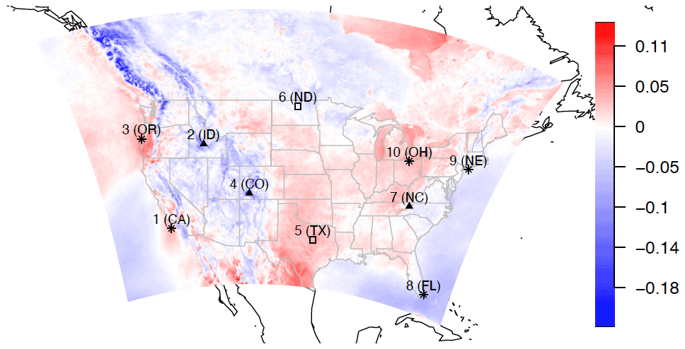
Figure 1Studied locations are the Californian coast (location 1), Idaho (ID) inland (location 2), Oregon (OR) coast (location 3), Colorado Mountain (location 4), Texas southern Great Plains (SGP; location 5), North Dakota Great Plains (location 6), southeastern mountains (location 7), Florida (FL; location 8), northeastern coast (location 9), and Lake Erie, Ohio (OH; location 10). We use the ∗ symbol to denote an offshore location, ▴ to denote a mountain location, and □ to denote a plain location. The map is colored by the ratio of changes in the 10-year mean 95th percentile of the wind speed distribution projected by WRF and driven by the Community Climate System Model 4 (CCSM4). See the data description in Sect. 2.
2.1 Regional climate model outputs
We use three WRF simulations driven by Community Climate System Model 4 (CCSM4; Gent et al., 2011), the Geophysical Fluid Dynamics Laboratory Earth System Model 2 (GFDL-ESM2G; Donner et al., 2011), and the Hadley Centre Global Environment Model version 2 (HadGEM2-ES; Jones et al., 2011). These three GCMs represent a range of climate sensitivities that encompasses most of the Coupled Model Intercomparison Project – Phase 5 (CMIP5) GCMs when projecting future temperature changes (Sherwood et al., 2014). For more details on these simulations, see Wang and Kotamarthi (2015) and Zobel et al. (2018a, b). The WRF outputs are instantaneous data taken every 3 h, which may capture some peak wind speeds, as they are not averaged over time; however, under this time resolution, intermediate gusts may have been missed. We consider wind at 10 m that is diagnosed from the higher simulated heights with the first layer simulated at 28.8 m.
In both CCSM4- and GFDL-driven WRF runs, boundary conditions are bias-corrected using reanalysis data, and nudging techniques are applied to WRF runs. No bias correction or nudging is applied to the HadGEM-driven WRF runs. In this work, we focus on historical data and the RCP8.5 scenario for future projections, which assumes the continued heavy use of fossil fuels at a similar, or greater, rate to the current concentrations of CO2 and other greenhouse gases (GHGs) through the end of the century, leading to a radiative forcing of 8.5 W m−2 by 2100 (Riahi et al., 2011). For the historical time period, we focus on 1995–2004, and for the future time period, we focus on the late 21st century period (2085–2094).
A 10-member ensemble of 1 year of RCM simulation using a bias-corrected CCSM4-driven WRF is also generated for analyzing the uncertainty due to the RCM's internal variability (IV; see the methods in Sect. 3.5) and for analyzing how significant the climate change signal in wind speed is when compared with this uncertainty. These ensemble members use exactly the same model configuration, such as physics parameterizations, spatial resolutions, and nudging techniques, except that their initial conditions are perturbed initial conditions. Further details about the experiment design can be found in Wang et al. (2018). Previous studies found that the IV was neither affected by the time period (i.e., historical versus future) nor by the type of driving data (i.e., reanalysis data versus GCM output; Braun et al., 2012). Lucas-Picher et al. (2008) found that, from a 10-member ensemble of 30-year simulations over North America, there was no long-term tendency in the IV, but there were fluctuations in the IV in time, such as in the day-to-day variations. Therefore, 1 year of ensemble simulations driven by one GCM is considered sufficient for our purpose in order to compare the magnitudes of future change in wind speed versus the uncertainty due to IV. See Sect. 3.5 for details describing the calculation of IV in this study.
2.2 Benchmark data
2.2.1 Reanalysis fields
Reanalysis data are used as a verification dataset to evaluate the RCM wind conditions under study for the historical time period. Only a few reanalysis datasets are available at high resolution and with both wind speed and wind direction. For the seven inland locations, we use the second phase of the multi-institution North American Land Data Assimilation System project, phase 2 (NLDAS-2; Xia et al., 2012a, b), at a spatial resolution of 12 km and hourly resolution. NLDAS-2 is an offline data assimilation system featuring uncoupled land surface models driven by observation-based atmospheric forcing. The non-precipitation land surface forcing fields for NLDAS-2 are derived from the analysis fields of the National Centers for Environmental Prediction (NCEP) North American Regional Reanalysis (NARR; Mesinger et al., 2006). NARR fields are spatially interpolated to the finer resolution of the NLDAS one-eighth of a degree grid and then temporally disaggregated to the NLDAS hourly frequency. Since NLDAS fields are not available offshore, we use NARR fields to evaluate the RCM wind conditions for the offshore locations. NARR reanalysis fields are at a 32 km spatial resolution and a temporal frequency of 3 h.
Because NARR data and reanalysis may present bias, we also consider in situ measurements described in Sect. 2.2.2. Pryor et al. (2009) advocate the use of multiple sources of datasets, while pointing out discrepancies between observations, RCM outputs, and reanalysis in their temporal trends of surface wind speed. In particular, reanalysis data show contradictory temporal trends from the observational and RCM data. Daines (2015) and Daines et al. (2016) also noted discrepancies between observational and NARR reanalysis along coastal British Columbia and posited the cause to the misrepresentation of the topography in NARR or a need for more assimilation of the near-surface wind speed.
2.2.2 In situ measurements
Since reanalysis data can present errors and uncertainties, ground measurements and offshore buoy measurements described below are used to consolidate the evaluation of RCMs' wind conditions for inland and offshore locations in historical climates.
Observational data are extracted from the Automated Surface Observing System (ASOS) network that consists of a station network covering the U.S. territory. Wind data are outputted every minute; however, wind speed are 2 min window averages of 5 s measurements. The recorded wind speed is discretized in integer knots (one knot is 0.514 m s−1). We do not apply any additional treatment to account for this discretization because the data are filtered (averaged) over a window of 1 h. Finally, ASOS data are often used for aviation purposes and, hence, are known to be high-quality data. ASOS data undergo three levels of quality checking during their creation (on-site and real-time checks before observation transmission, aerial or state checks by a weather forecast office (WFO) within 2 h after observation transmission, and a nationwide check about 2 h after the scheduled transmission time).
The offshore downscaled wind speeds from the historical decade are compared with National Data Buoy Center (NDBC) buoy observations of near-surface wind velocities. The observed winds at the NBDC anemometers are collected at an hourly rate averaged from 8 min observations. The data are extrapolated to 10 m above ground height through the power law extrapolation method (Hsu et al., 1994), following , where WSNDBC is the wind speed directly from the buoy, and hNDBC is the buoy sensor elevation between 3.8 and 4.1 m, depending on the buoys. The exponent of 0.11 is an empirically derived coefficient, based on the stability of the atmosphere, for water conditions in this study.
In the following, we perform a station-wise comparison of wind speed and direction and select locations across the country with various climatic conditions. For each selected location, we consider the closest grid points from each model and the closest in situ data measurements.
This section describes the statistical techniques used for modeling the probability distributions of wind direction and wind speed conditioned on direction. Due to the circular nature of the wind direction variable, we fit a von Mises mixture distribution (Fisher, 1995; Mardia and Jupp, 2009; Breckling, 2012) to the wind directions, and we model the wind speed distribution conditioned on the wind directions by two distributional regression models, i.e., (1) quantile regression (Koenker and Bassett, 1978) and (2) a two-step Weibull distributional regression model, both of which impose a circular constraint. In the following, we give a brief account of the von Mises mixture distribution, our two-step Weibull regression, and quantile regression, respectively.
3.1 Von Mises distribution
The von Mises distribution (also known as the circular normal distribution) has been widely used to accommodate the circular nature of wind direction. The probability density function of the von Mises distribution is given by the following:
where I0(κ) is the modified Bessel function of the order 0 (Hill, 1977), μ is the location parameter that describes where the bulk of the angle x distribution is clustered around, and κ measures the level of concentration around the location μ (the larger the κ, the more concentrate the data to μ), so is analogous to σ2 in the normal distribution.
The von Mises distribution is unimodal and may lack the flexibility to capture the potentially complex wind direction distribution. Therefore, we employ a two-component mixture of von Mises distributions that can accommodate more complicated wind direction distributions while keeping model fitting manageable, using the movMF package developed by (Hornik and Grün, 2014) in R. The probability density function of the von Mises distribution mixture is given by the following:
and its parameters are estimated via the expectation–maximization (EM) algorithm (Dempster et al., 1977).
3.2 Periodic quantile regression
Quantile regression (QR) extends the scope of classic regression analysis, which models the conditional mean of a response (𝔼(Y)) as a function of the explanatory variables x's, to modeling how a quantile of a response changes with the explanatory variables (Koenker and Bassett, 1978). Since the quantile functions fully determine the distribution FY, one can estimate a set of conditional quantile levels (i.e., , , x∈ℝ) to approximate the underlying conditional distribution. By doing so, one can obtain a more complete picture of the full distribution of interest and how this distribution varies with the predictors (Mosteller and Tukey, 1977). More details can be found in the Appendix A.
In this study, we model a given quantile of wind speed varying across wind direction by representing the directional quantile curve as a periodic B spline. We utilize the quantreg and pbs packages in R to implement this procedure. Having a collection of estimated conditional quantiles will provide us with information on not only how a specific quantile level of wind speed changes with direction but also how these quantile curves, as function of wind direction, change across quantile levels.
3.3 Weibull distributional regression
The Weibull distributional regression (WDR), an example of parametric distributional regression (Kneib et al., 2021) with the Weibull conditional distribution assumption, is another method that we propose for estimating wind speed quantiles conditioned on direction. Under Weibull distribution assumptions, we need to estimate how the scale λ and shape κ parameters vary as functions of wind direction ϕ with periodicity constraints. We propose a two-stage procedure as follows: (1) we bin the data by dividing the wind direction into N bins, and then fit a Weibull distribution to the wind speed data within each bin via maximum likelihood method to obtain the estimates and their standard error . (2) Next, we estimate λ(ϕ) and via a harmonic regression (i.e., , and ). Specifically, with a chosen K, we fit, by weighted least squares, to and to obtain , where the weights are the reciprocal of squared standard errors, and is the average wind direction within the jth bin. The use of harmonic regression here ensures both λ(ϕ) and κ(ϕ) are circular functions.
Although the Weibull distributional regression and quantile regression are both employed in this study to estimate wind speed quantiles conditioned on direction, there are some distinctions between the two methods. Both methods use the wind direction as a predictor of the wind speed. For the binning of the wind direction in this study, quantile regression represents each bin with the same amount of data and, hence, each bin has different length, whereas bins in the Weibull regression have the same length, and thus each bin contains different number of data points. In this study, binned Weibull fitting performs slightly better than quantile regression, except at the Idaho (ID) location, due to very unstable parameter estimates for one of the direction bins (only a few data points are contained in that bin). An ongoing study on assessing the estimation performance via Monte Carlo simulations of these two methods can be found in Murphy et al. (2022).
3.4 Quantify estimation uncertainty via bootstrap
For both QR and WDR, we use bootstrapping (Efron and Tibshirani, 1994) to quantify the uncertainty associated with the parameter estimation. Specifically, we draw 500-block bootstrap samples, where the block size is taken to be one season to preserve the temporal dependence within a season. The upper and lower percentiles of the bootstrap distribution are used to form a confidence interval to quantify estimation uncertainty (see Fig. 2, for an example). In Sects. 5 and S3, we provide confidence intervals for other selected locations.
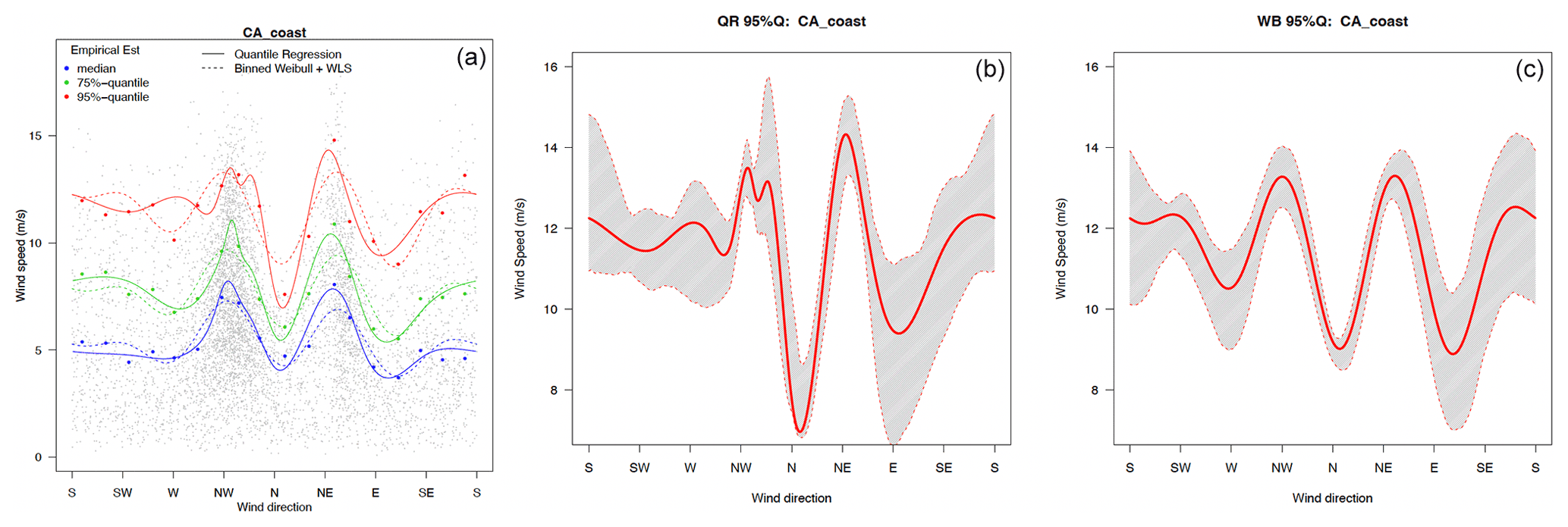
Figure 2WRF-CCSM winter California (CA) coast data. (a) Fitted quantile curves (50th, 75th, and 95th quantiles) of the quantile and Weibull regression methods at the CA grid point, along with their bin-wise empirical estimates. (b) The 95 % bootstrapped confidence intervals of the 95th quantile (gray shaded area) and its point estimate (red curve), using periodic quantile regression. (c) Same as panel (b) but using Weibull regression.
3.5 Internal variability and projected climate change signal
In this section, we propose new statistics based on the commonly used internal variability (IV). IV arises from intrinsic variations in the nonlinear physical and dynamical processes that are described by climate models (Hawkins and Sutton, 2009; Wang et al., 2018). Due to the restrictions on the large-scale atmospheric flow imposed by the lateral boundary conditions, the level of IV generated by RCMs is smaller than those generated by GCMs (at least at the large scale). However, it is important to evaluate the IV of an RCM because this variability may modulate or even mask physically forced signals in the model (Braun et al., 2012; Deser et al., 2012). In order to assess the strength of climate change signals relative to the internal variability in the system, we compare the intensity of the climate change signal to the IV of the WRF model. The IV is typically calculated by the time-wise spread across members of an ensemble averaged over given time windows. Members of an ensemble are commonly started with perturbed initial conditions.
The IV usually represents the average over a time window 𝒯, where 𝒯 represents days, months, or seasons of the time-wise ensemble spread, as follows:
where refers to a variable Y on grid point (i,j) at time t and the member n in the N ensemble. In this study, we consider N=10 members (described in Sect. 2.1) and compute the IV over the summer and winter time windows for data taken every 6 h.
The commonly used IV provides information on the ensemble variability with respect to the mean of the quantity of interest; however, it does not provide information regarding the internal variability in other summary statistics, such as its variance or quantiles. This study extends the concept of IV to compute the ensemble spread of the standard deviation and 95th quantile of the wind speed. For the IV of the standard deviations, we calculate the spread across ensemble members of the wind speed standard deviation, as follows:
where is the standard deviation of the ensemble member n at location (i,j) for the season 𝒯, and
where . Similarly, for the 95th quantile IV, we calculate the 95th quantile value of each ensemble member n over a season 𝒯, and then we calculate the ensemble spread of the member 95th quantiles, as follows:
where is the 95th quantile of the ensembles over a season 𝒯.
When projected climate changes (PCCs), which are derived as the difference between historical and projected statistics, are 2-fold larger than the internal variability, changes can be considered robust with respect to the IV (Wang et al., 2018). These computations are performed on the WRF-CCSM ensemble (described in Sect. 2.1).
In this section, we evaluate the historical RCM outputs against reanalysis data and in situ measurements (as described in Sect. 2) via different statistical methods (described in Sect. 3).
4.1 Comparison of reanalysis benchmark data and in situ measurements
First, we evaluate the reanalysis benchmark data NARR, using in situ buoy observation over coastal locations, and the reanalysis benchmark data NLDAS, using near-surface observation ASOS data over inland locations.
Buoy data are reported hourly and are averaged based on 8 min measurements, while NARR and WRF outputs are instantaneous outputs taken every 3 h. As a result, NARR and WRF may capture some peak wind speeds, while the buoy data may smooth out peaks. However, because NARR and WRF only output data every 3 h, they likely miss peaks during these 3 h intervals.
Figure 3 shows the diurnal patterns of wind speed for three offshore locations (the California (CA) coast, NW coast, and NE coast) of NARR reanalysis and buoy measurements. NARR captures the seasonal differences between summer and winter wind speed shown in buoy data, e.g., winter has a stronger wind speed than summer does in offshore locations in the northwest and northeast. The diurnal pattern of the wind speeds over the CA coast is also captured by NARR. However, for both summer and winter wind speed, NARR tends to underestimate the wind speeds compared with buoy measurements. On average, at the CA coast location, NARR underestimate buoy wind measurements by around 2.2 m s−1 (29 %, relatively speaking) in winter and 4.6 m s−1 (48 %, relatively speaking) in summer. At the NW coast, the underestimate is around 1.4 m s−1 (17 %, relatively speaking) in winter and 0.4 m s−1 (8 %, relatively speaking) in summer. At the NE coast, the underestimate is around 1.2 m s−1 (13 %, relatively speaking) in winter and 1.2 m s−1 (22 %, relatively speaking) in summer. In a later section, we observe the systematic low bias of NARR compared with WRF. The wind speed over the CA coast in winter is underestimated in NARR by about 4 m s−1. This misrepresentation of wind along the coast may corroborate the results from (Daines, 2015; Daines et al., 2016) on coastal wind misrepresentation by NARR data, and we also note that the NARR spatial resolution is coarse (32 km), inducing a different quality of results at the grid cell level. Figure 4 shows the diurnal patterns from ASOS and NLDAS data, using three inland locations over the U.S. in 2018 January, February, June, and July. Overall, we find that NLDAS reanalysis data captures both wind speed and direction well. We have also evaluated other locations across the CONUS and find that NLDAS provides a reasonable benchmark dataset for the selected inland locations.
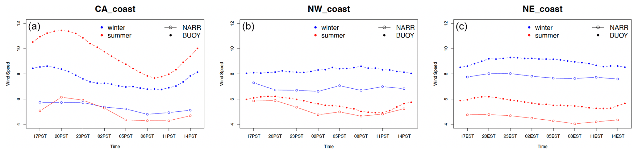
Figure 3Diurnal wind speed pattern of NARR and buoy wind data for the three offshore locations on the CA coast, NW coast, and NE coast (from left to right), displayed in winter (blue) and summer (red). Diurnal cycles are computed as averages over 10 years (1995–2004).
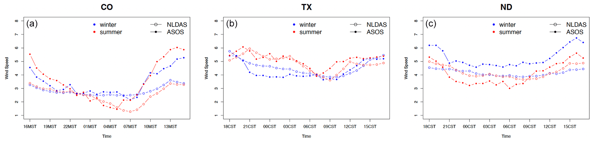
Figure 4Diurnal wind speed pattern of NLDAS and ASOS wind data for the three inland locations in Colorado (CO), Texas (TX), and North Dakota (ND), from left to right, displayed in winter (blue) and summer (red). Diurnal cycles are computed as the averages of January and February 2018 for winter and June and July 2018 for summer.
4.2 Wind direction evaluation
Figure 5 shows von Mises density estimates for an inland Texas–southern Great Plains (Texas-SGP) location in winter (right) and an offshore location of the CA coast in winter (left). The estimated von Mises densities for the remaining locations can be found in Sect. S1 in the Supplement. In general, WRF simulations driven by different GCMs were able to capture the distribution of wind directions well over most locations. For example, over the CA coast, the wind direction is dominated by the westerly and northwesterly winds in both summer and winter, which is driven by the high-pressure system over the mid-latitude Pacific. Over Texas-SGP, the winter winds have two dominant directions (southerly and northerly), which are well captured by the mixture of von Mises distributions, and the summer winds have only one dominant direction that is caused by low-level jet from the Gulf of Mexico to the Great Plains and eastern U.S. One exception is that none of the WRF simulations capture the wind direction distribution well over Colorado Mountains, likely due to the high elevation and high spatial variability in the terrain conditions that are not well modeled by the current spatial resolution in WRF.
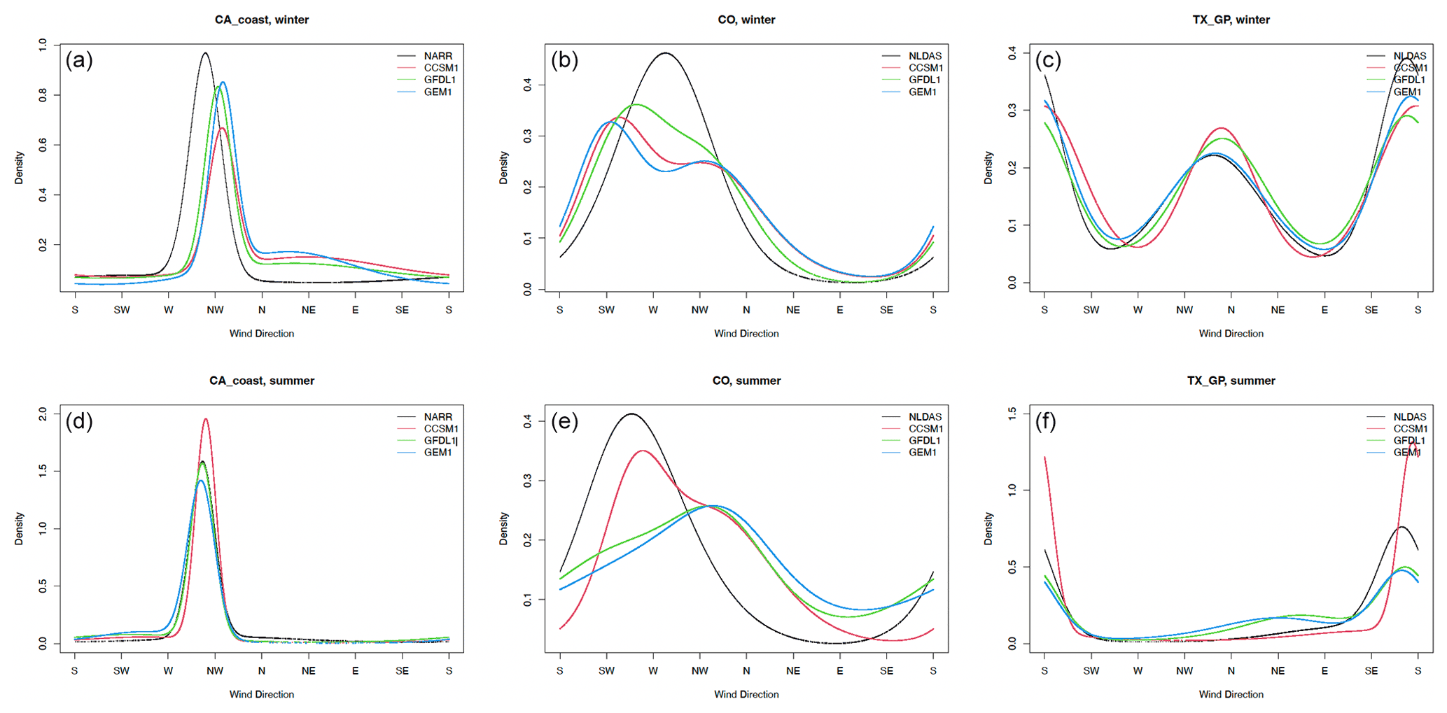
Figure 5Fitted von Mises mixture densities for historical data. From left to right is offshore California, Colorado, and Texas-SGP. From top to bottom is winter and summer. The black, red, green, and blue curves represent the benchmark (NARR for offshore and NLDAS for inland), WRF-CCSM, WRF-GFDL, and WRF-HadGEM models.
4.3 Wind speed distribution conditioned on direction
We use the quantile regression with periodic B splines to estimate the median and 95th quantile of wind speed conditioned on wind direction. Figure 6 compares the binned WDR and quantile regression results using WRF and NLDAS over CO and Texas-SGP inland locations and WRF and NARR at the CA location in winter. (Results for the remaining locations can be found in Sects. S4 and S5.) For the offshore location on the CA coast (left panel), both the median and the 95th quantile in the benchmark data NARR show the strongest wind speed concentrated in the northwesterly directions, which is favorable for stable wind resources. All three WRF models capture high wind speeds in the western and northwestern direction but also generate high wind speeds in northeastern and eastern directions that are not present in the NARR data. In addition, WRF simulations tend to overestimate wind speed by 1 to 5 m s−1 (1 % to 25 % of relative change) compared to NARR and NLDAS for most the directions. According to the validation of NARR, using buoy data in Fig. 3, the apparent overestimation could mostly be coming from the systematic low bias of NARR. For example, over the CA coast, the wind speed is underestimated in NARR by about 4 m s−1. Therefore, the overestimation seen in Figs. 6 and 7 over the CA coast is not as concerning as it appears. Over the Colorado location, WRF simulations capture the highest wind speed in southern and southwestern directions and the lowest wind speed in the northeast and east. Over the Texas location, WRF simulations capture the highest wind speed in the northwest and north in addition to the magnitude of the wind speed, indicating that reanalysis benchmark data and WRF simulations show a strong consistency. Note that winds are relatively easier to simulate in flat regions than over complex terrains such as mountains and coastal lines. WRF-simulated dominant wind directions over the Texas and Colorado locations are similar overall to the ones from NLDAS.
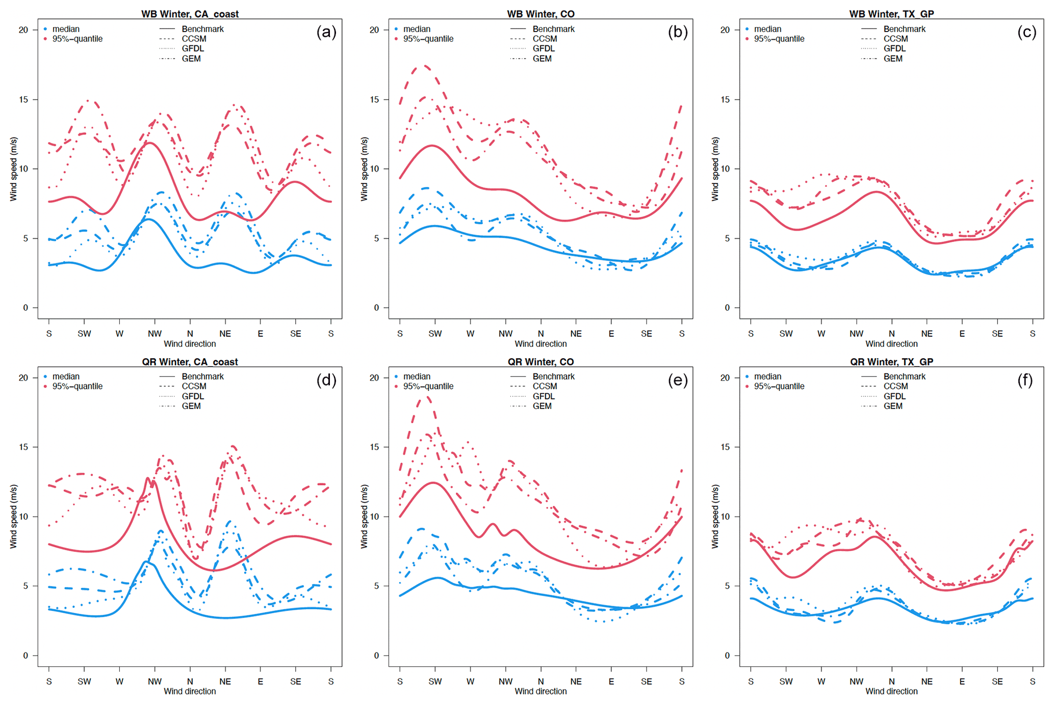
Figure 6The 50th (blue) and 95th (red) quantiles of wind speed as a function of wind direction for the historical period in winter for offshore California (a, d), Colorado (b, e), and Texas-SGP (c, f) using the Weibull distribution regression model (a–c) and quantile regression model (d–f). The different RCMs are shown with different types of dotted and dashed lines, while benchmark data are in solid lines (NARR for offshore and NLDAS for inland).
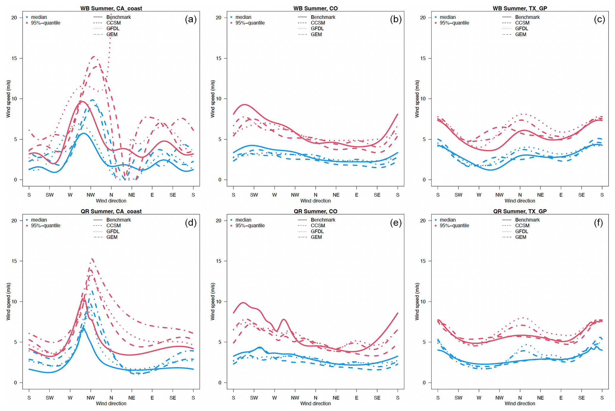
Figure 7 shows the binned WDR and quantile regression results for WRF and benchmark data over the same location as shown in Fig. 6 but in summer. While the two inland locations have much weaker wind speeds in summer than in winter, the offshore location over CA shows a similar high wind speed (95th quantile); however, its median wind speed is stronger in summer than in winter. WRF outputs capture the dominant wind direction over all three locations. Interestingly, the highest wind speeds over all three locations are located in the same direction as seen in winter. For example, over the offshore location in CA coast, the highest wind speed is concentrated over the northwestern locations. More importantly, although WRF models show three peaks of wind direction in winter, the benchmark NARR data demonstrate only one peak, which is the same direction peak as the summer scenario. Over the inland locations, the highest wind speed is from the southern and southwestern directions over the Colorado location and northern and southern over the location in Texas. This is perhaps encouraging information for wind energy resource development, as stable wind directions can ensure stable wind energy production. One potential reason for the inconsistency could be the resolution difference, as NARR has a 32 km resolution, while WRF has a 12 km resolution. A mismatch in the locations at the grid point level is typically more visible for offshore locations. Another reason for the direction bias could be that mountain areas are more sensitive to the wind direction.
In order to better quantify the results, we calculate a weighted integrated average of the relative error (WIRE) of the estimated distribution of model output (mod) with respect to the estimated distribution of reanalysis (obs). The weights are coming from the wind direction density of the reanalysis data, as follows:
where ϕ represents wind direction, and r represents wind speed. f(⋅) represents the corresponding models (QR or WDR for wind speed and von Mises distribution for wind direction), and t(ϕ) represents the density of the wind direction. Table B1 in Appendix B provides the WIRE for all stations in winter and summer seasons during 1995–2008 at 95 % quantile level via quantile regression, Weibull directional models for wind speed, and von Mises distribution for wind direction. Taking Fig. B1 as an example, when WIRE is high, such as in the example where the CCSM at CO in winter from the quantile regression is 0.407, we can see the huge discrepancy between the CCSM and the benchmark curve at the southwesterly direction, where the wind direction density is the highest. When WIRE is small, such as in Texas-SGP in winter for which quantile regression is 0.132, the curves are very close to each other.
In this section, we focus on projections of wind conditions in the late century (2085–2094) under the RCP8.5 scenario compared with wind conditions in the historical period (1995–2004). We also conducted the same analysis using mid-century projections, and the climate change signal is smaller but the conclusions are qualitatively similar (not shown). The changes in wind speed distributions conditioned on direction are estimated using quantile regression and Weibull distributional regression, where a bootstrap (Sect. 3.4) is used to quantify the estimation uncertainty. We also compute their projected changes for the mean, standard deviation, and 95th quantile of wind speed and compare them with the corresponding statistics of internal variability defined in Sect. 3.5. Finally, in addition to the near-surface wind, we also discuss the uncertainty due to internal variability versus projected changes in wind conditions at higher heights relevant to wind industry (up to 200 m) in WRF outputs to shed some light on potential future changes in wind energy resources.
5.1 Changes in wind speed and direction distributions
The change in wind direction estimated by a von Mises distribution between the historical and late century periods is not significant in all the locations (as shown in Sect. S1). Thus, in the following, we focus on the change in the wind speed conditioned on direction. Figure 8 shows the estimated wind speed quantiles (50th, 75th, and 95th) conditioned on direction for WRF-HadGEM outputs at the CO mountain location in winter, using both quantile regression and Weibull distributional regression (upper panels), and the associated 95 % pointwise bootstrapped confidence interval (for the 95th quantile), using the Weibull distributional regression. The corresponding results for the remaining nine locations can be found in Sect. S2. Compared with the wind speed quantile estimates conditioned on the direction from the historical period, the projected winds at the Colorado Mountains location show evident weaker wind speeds conditioned on direction, especially for the dominant wind direction southwesterlies, but also other directions such as westerlies and northwesterlies from both the quantile regression and Weibull distributional regression models at all three quantiles. Figure 9 shows similar statistics for the northern Great Plains location in North Dakota, and the prevalent wind directions tend to be similar from the historical to the late century periods. The overall wind speed tends to show a decrease in intensity (across all quantiles) in particular in the dominant direction mode.
We also find that the dominant wind speeds conditioned on the direction decrease at the Idaho inland location and Florida (FL), as shown in Sect. S2. In addition to the wind speed change at the dominant wind directions, there are changes in future wind speed patterns conditioned on the direction. For example, at the Oregon (OR) coastal location during the historical period, the northwesterly winds are dominant at both median and high wind speeds; in the projections, there are stronger winds from the southeasterly direction as well. Over Lake Erie, in the historical period, the dominant wind speeds are southwesterly and northeasterly; in the future, the northeasterly wind will decrease while the northerly wind will increase. In summary, the change in the median winds from the historical to the late century periods is noticeable in some locations such as the Colorado Mountains and Idaho inland but minor in most locations. However, the 95th quantile wind speeds conditioned on direction tend to show more changes. These changes in the conditional wind 95th quantile are corroborated by the unconditional changes in the 95th quantile winds observed in Fig. 1, where most regions of the U.S. exhibit changes in their 95th quantile winds with up to around 20 % decrease and up to around 12 % increase in 95th quantile across all wind directions.
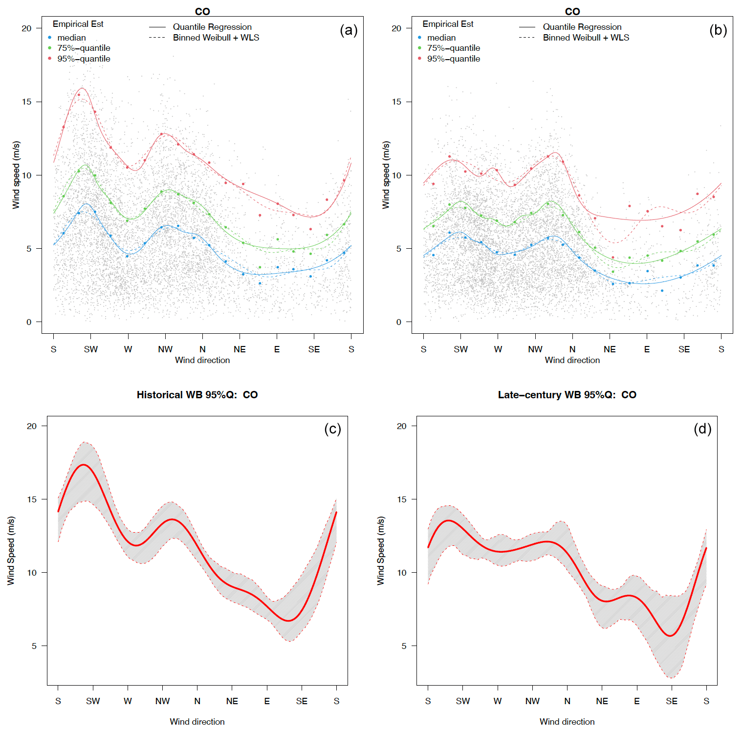
Figure 8Estimated wind speed quantiles (a, b; blue for the 50th, green for the 75th, and red for the 95th quantile) conditioned on wind direction and their bootstrapping estimation uncertainties (c, d; only results for the 95th quantile are shown) at the Colorado Mountains grid cell for the winter season under the historical (a, c) and late century periods (b, d).
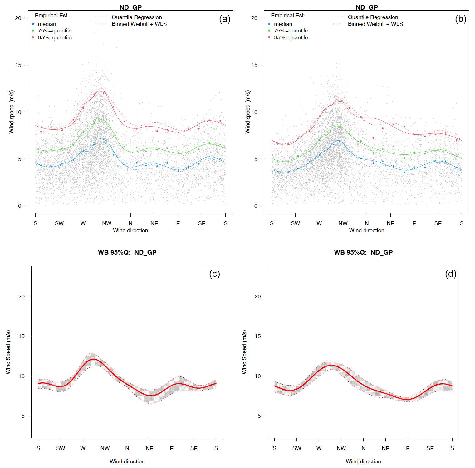
Figure 9Estimated wind speed quantiles (a, b; blue for the 50th, green for the 75th, and red for the 95th quantile) conditioned on wind direction and their bootstrapping estimation uncertainties (c, d; only results for the 95th quantile are shown) at the northern Great Plains (NGP) grid cell for winter season under the historical (a, c) and late century periods (b, d).
5.2 Projected climate change versus internal variability
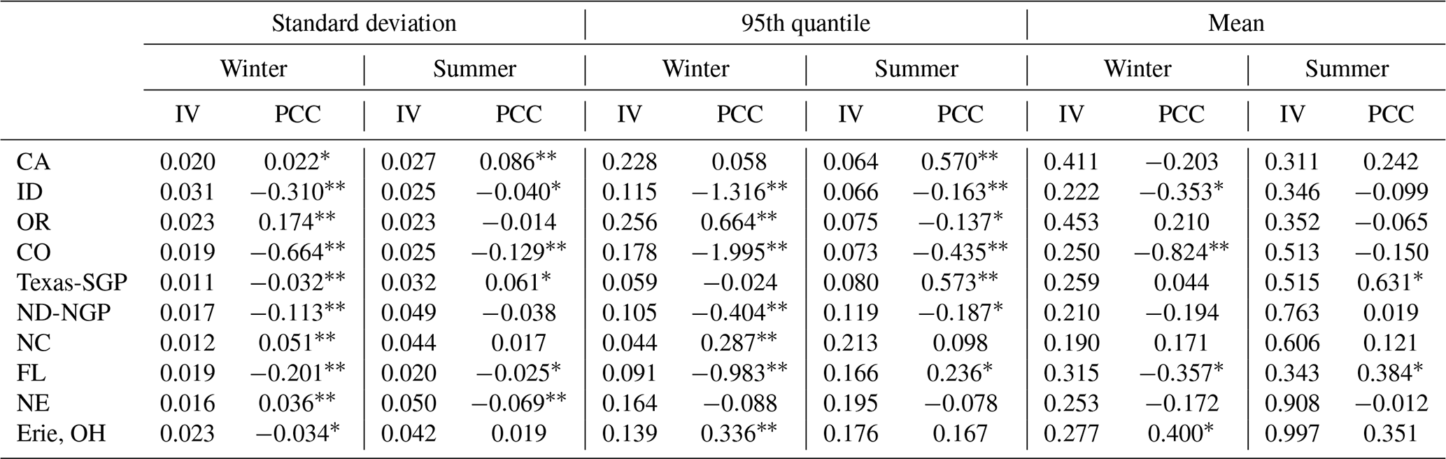
From previous discussions, we noticed that several locations may show a general decrease in the wind speed at their dominant wind directions, while other locations may experience changes in the dominant wind directions themselves, yet other locations do not exhibit any significant wind condition changes in the late century period. In this section, we investigate the robustness of such projected changes by considering the uncertainty due to the internal variability (Wang et al., 2018) that is caused by a perturbation in the initial conditions. We calculate the commonly used internal variability and the newly defined internal variability for standard deviation and 95th quantile (following Sect. 3.5), and the results are summarized in Table 1. These IV statistics enable the assessment of the significance of projected changes over the intrinsic variability in the models for other statistics (standard deviation and 95th quantile) than the commonly used mean statistics. Table 1 provides insights to significant changes across the seasons, locations, and statistics of the wind speed. Across the three studied statistics, winter shows the most significant changes in the wind speed statistics. In particular, the standard deviation and 95th quantile show the most changes in intensity across locations compared to mean wind speed, namely that the winter standard deviations and 95th quantiles mostly show a decrease between the historical and late century conditions. In contrast, the summer 95th quantiles tend to show some increases in the wind speed statistics.
Table 1The 10-year-based IV and PCCs from WRF-CCSM. The asterisk indicates , and the double asterisk indicates . Note: NC is North Carolina.
In the following, in order to generate the observed variability in PCCs and gather more information on PCCs than a single a PCC statistic (difference between the historical and projected statistic), we compute the PCC differences in yearly statistics. Figure 10 presents the yearly PCC variability (box plot) and the internal variability (red lines) over the 10 studied locations across the U.S. for the standard deviation and 95th quantile in winter and summer. First, we calculate the standard deviation and the 95th quantile of each year in the historical (1995–2004) and future (2085–2094) periods and consider all the differences between historical and projected statistics. The box plot (box, whiskers, and black line for the median) shows the distribution of these differences (yearly historical and yearly projected) for the seasonal standard deviation and seasonal 95th quantile. In each case, the internal variability is added and subtracted to the median values of standard deviations and 95th quantiles. When the difference between the median of historical and future is 2 times larger than the internal variability, then we consider the climate change in standard deviation and 95th percentile of wind speed to be significant with respect to the internal variability.
We observe that, in winter, the standard deviation is reduced by 0.1 to 1 (5 % to 20 % of the relative change) in the late century period over seven locations, especially over the northwestern inland location (location 2), Colorado Mountains (location 4), and Lake Erie (OH; location 10), where the standard deviations are reduced robustly, indicating that the variability in the winter wind speed in the projections over these locations are smaller or simply that the wind speed in the future winter is weaker. The projected high wind speed (95th percentile) over these locations also show a robust decrease (top right panel), suggesting lesser wind energy resources in the future. In summer, both the yearly PCC variability and the projected changes in the standard deviation and 95th quantiles are relatively small compared to those statistics in winter. There are slight increases in the standard deviation and wind speed 95th quantile over CA offshore (location 1) and the Texas Great Plains (location 5); however, these increases are not significant compared with the internal variability.
Table 2Relative changes in different quantiles for CCSM-4 data in winter between projected period (2085–2094) and historical period (1995–2004). Quantiles are estimated with a Weibull distributional regression, WDR (a), and quantile regression, QR (b).
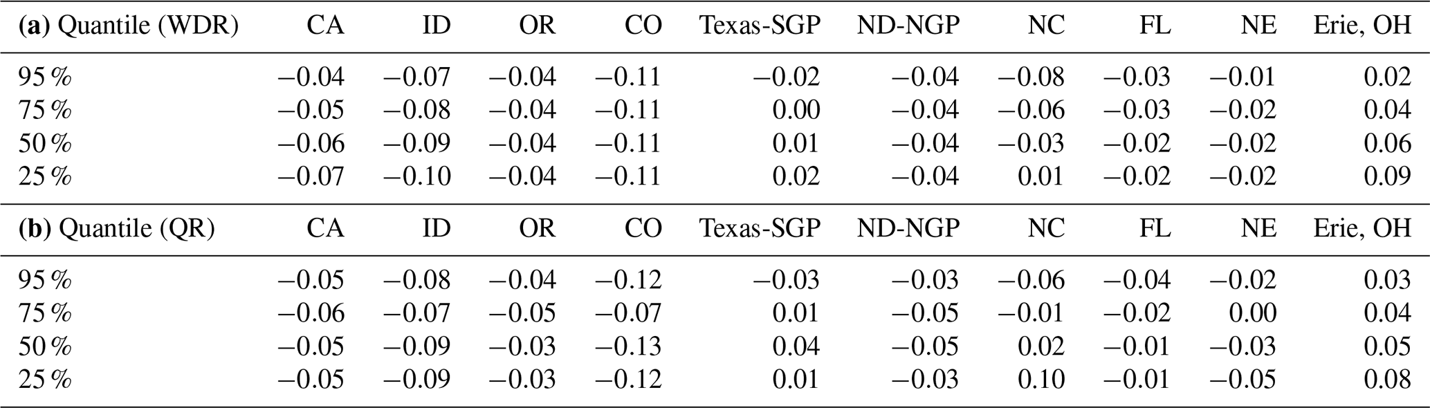
Finally, we provide, in Table 2, the percentages of the relative changes between the historical and late century periods of the 25th, 50th, 75th, and 95th quantiles estimated by both the Weibull distributional and quantile regression models for winter in order to provide additional information to the winter changes. We notice that the lower the quantiles, the smaller the relative change will be. In most cases of changing wind quantiles, several quantiles are affected simultaneously with different rates and signs of changes, suggesting a more complex distortion of the wind distributions than simple shifts. In particular, some stations like Texas-SGP and North Carolina (NC) exhibit a stretch in the 25th quantile but a contraction in the upper tail.
To explore the future changes in wind speeds at higher heights (e.g., wind turbine hub heights), we have conducted the same analysis for three higher heights above the ground level, at 28.48, 97.88, and 192.39 m, from the WRF runs. We found similar conclusions to the near-surface wind speed (results are not shown). That is, while the mean wind speed change is not robust with respect to the internal variability, the changes in the standard deviation and 95th quantile are robust over certain locations in winter. For example, the wind speed is projected to decrease over the northwestern inland and Colorado Mountains.
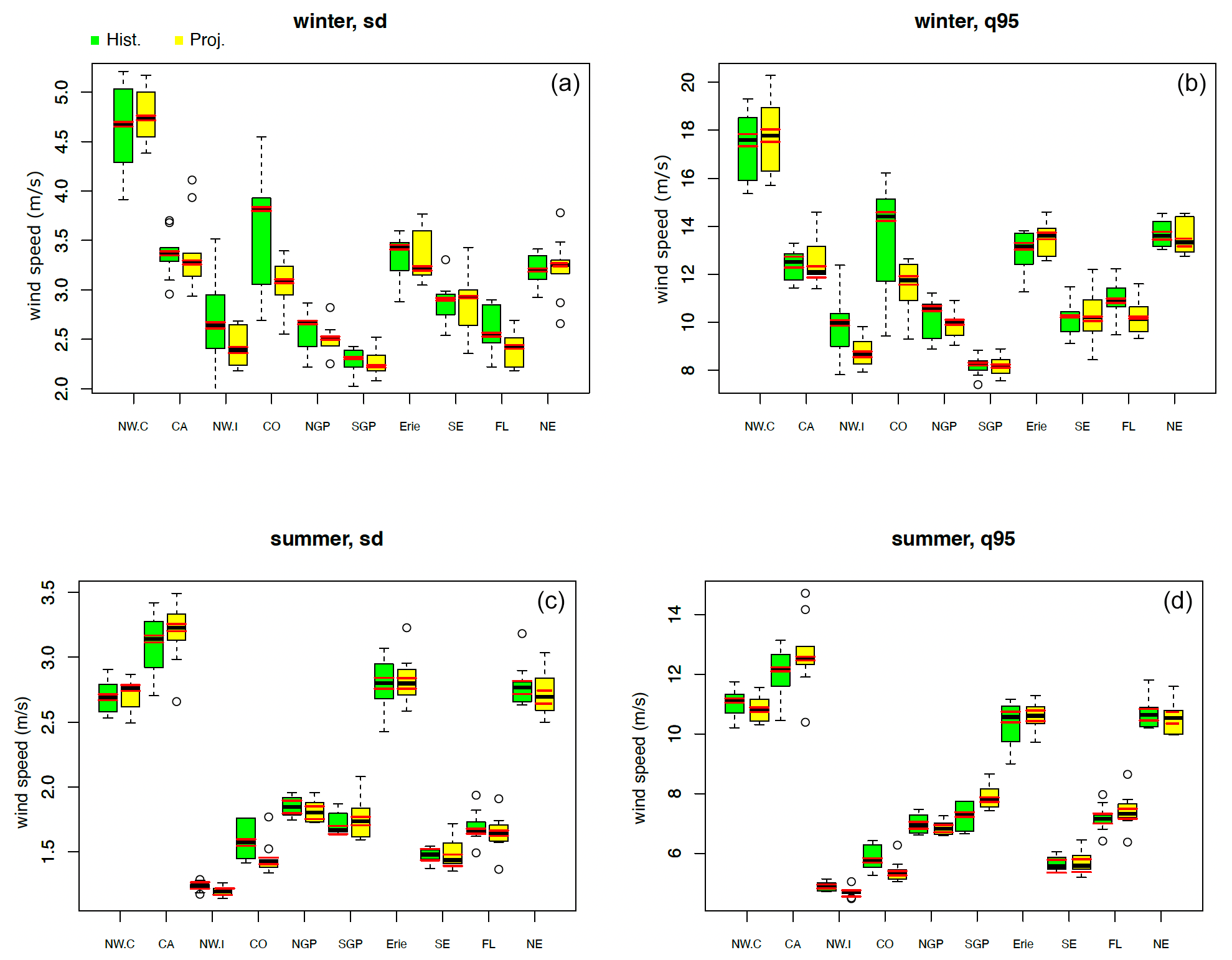
Figure 10Box plot of the standard deviation (a, c) and 95th quantile (b, d) yearly PCC variability with a corresponding IV in 10 locations from WRF-CCSM. The boxes and whiskers are statistics based on 1 year for 10 years in the historical and future periods, indicating the yearly PCC variability in each 10-year period. The red lines represent the median statistic ± the IV for each location. If the difference between the two means from historic and late century are larger than the IV, then we consider that the future changes in these statistics are robust.
In this work, we study wind conditions (speed and direction) and their potential projected changes via a statistical conditional framework, where the probability distributions of the wind directions are modeled via von Mises mixture distributions, and wind speed conditioned by direction distributions is characterized by two distributional regression models, namely the quantile regression and Weibull regression models. The proposed framework allows us to better characterize the wind direction distributions and wind speed distributions conditioned on wind direction and, hence, provides the full description of the joint wind speed and direction distributions. In addition, we investigate the strength of the projected wind speed distributional changes relatively to the interval variability in the climate models. The extension beyond the mean change to the changes and internal variability in standard deviation and 95th quantile provides a more complete picture for assessing the significance of their changes relative to their internal variability. Finally, future works may consider the spatial aggregates of these quantities to reduce the noise of climate variability and potentially observe stronger trends.
We also perform a comprehensive climate model evaluation, where RCM outputs are evaluated against reanalysis data and in situ measurements. Results from the WRF configurations are consistent in both wind direction and speed. Wind direction and speed in summer are generally less dispersed than the winter scenarios. We observe that the benchmark NARR and NLDAS data, corroborated by buoy and ground station data, are mostly consistent with the WRF outputs in most locations. Our evaluation study also highlights the challenges of finding appropriate benchmark data for these high-resolution RCMs in some situations (e.g., offshore and mountain areas). Few data products are available at high resolution, and in situ measurements are irregularly available in space with varying time resolutions.
This study concludes that the changes between the historical and future wind directions are usually small in the locations that we examined, but wind speeds are generally weakened in most of the locations we considered in the projected period, with some locations and directions becoming intensified in the future. The projected climate changes in the 95th quantile and standard deviation are significant over the internal variability at some locations and decrease in locations such as the northwestern inland area, Colorado, and Lake Erie, especially in the winter season.
The current implementation of our statistical framework has some limitations. First, both distributional regression methods require some tuning; the Weibull regression requires choosing the binning and determining the complexity regression functional form (via the number of the harmonic terms), whereas the quantile regression requires the selection of knots and the degree of freedom of the periodic B splines. Further statistical studies of these modeling choices can be found in Murphy et al. (2022). Second, all the statistical analyses are performed pointwise for simplicity, while spatiotemporal-dependent structures are not considered here. In order to assess the regional wind fields and their future predictability, it is critical to explore their spatiotemporal structures in future work.
In this work, we model the τ quantile of the wind speed (WS) conditioning on the wind direction (WD), using a quantile regression with periodic B spline. The estimator of takes the following form:
The vector Z(wd) is a periodic B spline with the degree of freedom s evaluated at wind direction value wd. The periodic B spline, instead of a more commonly used B spline, is used to preserve the periodic circular property of the wind speed distribution conditioned on wind direction. We select the degree of freedom (s=8) by finding the elbow point of the mean absolute error (MAE) of the regression residuals versus degree of freedom ratio. The coefficient vector is the QR estimator of β(τ), as follows:
where ρτ is a loss function for τth quantile. It can usually be expressed as follows:
We seek to minimize quantile loss by differentiating Eq. (A4) with respect to , as follows:
We propose a weighted integrated relative error (WIRE) of the estimated distribution of model output (mod) to the estimated distribution of reanalysis (obs). The weights are coming from the wind direction density of the reanalysis data.
where ϕ represents wind direction, and r represents wind speed. f(⋅) represents the corresponding models (quantile regression or Weibull WDR for wind speed and von Mises distribution for wind direction), and t(ϕ) represents the density of the wind direction. Table B1 provides WIRE for all stations in winter and summer seasons during 1995–2008 at the 95 % quantile level via quantile regression, Weibull directional models for wind speed, and von Mises distribution for wind direction. Taking Fig. B1 as an example, when WIRE is high, such as for CCSM at CO in winter for which the quantile regression is 0.407, we can see the huge discrepancy between CCSM and the benchmark curve at the southwestern direction where the wind direction density is the highest. When WIRE is small, such as for Texas-SGP in winter for which the quantile regression is 0.132, the curves are very close to each other.
Table B1Summary metrics with WIRE for all stations in winter and summer seasons during 1995–2008 at 95 % quantile level via quantile regression, Weibull directional models for wind speed, and von Mises distribution for wind direction.
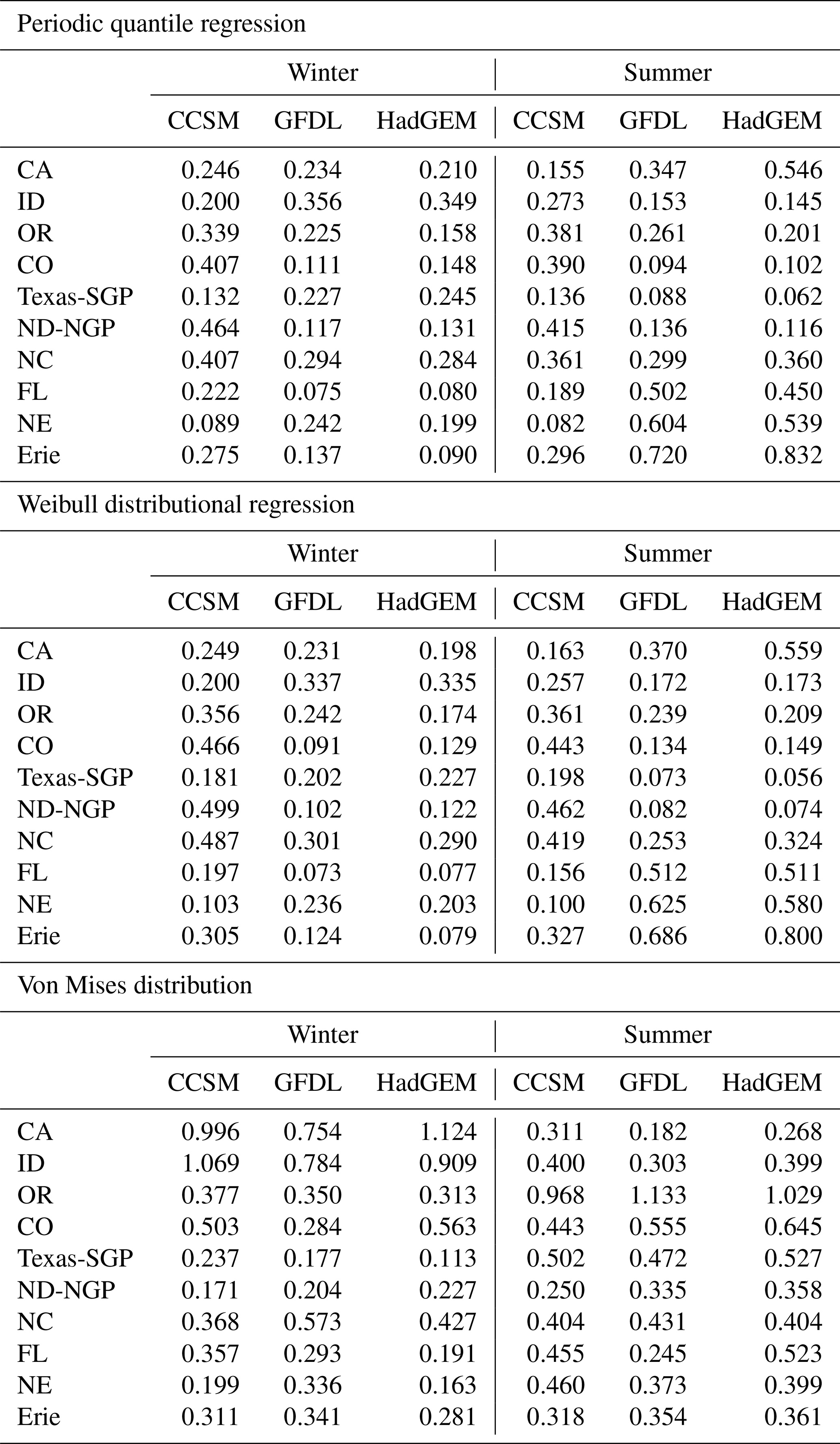
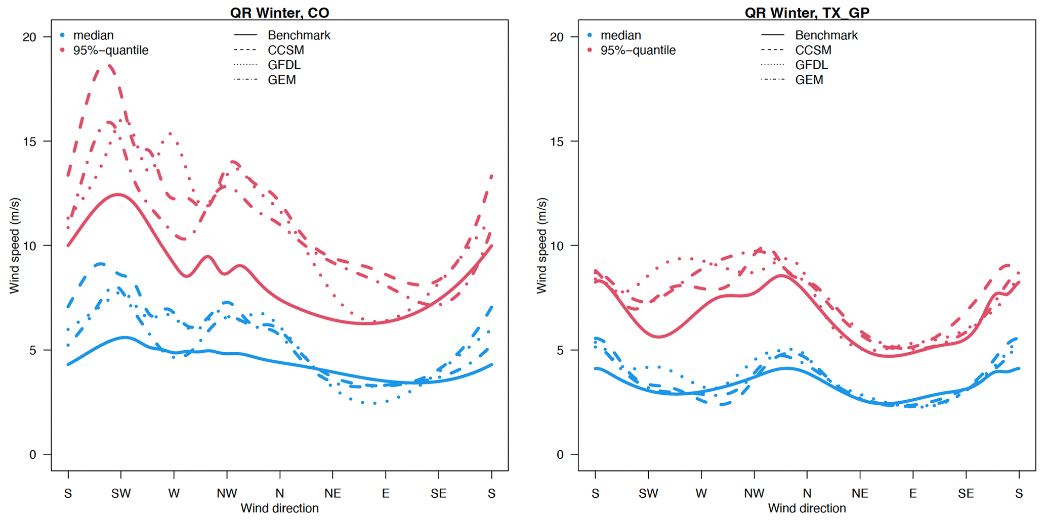
Figure B1Quantile regression in winter during 1995–2004 at two selected locations as an example for the summary metrics table.
The source code is available in the GitHub Wind Project repository https://github.com/QiuyiWu/Wind-Project (last access: 26 November 2022) and Zenodo https://doi.org/10.5281/zenodo.7358862 (Wu, 2022). The data used in this study are available at https://doi.org/10.5281/zenodo.6425797 (Wu et al., 2022).
The supplement related to this article is available online at: https://doi.org/10.5194/ascmo-8-205-2022-supplement.
QW participated in the entire project by the conducting data analysis and visualization of the study and prepared the original draft. JB proposed the idea of the project and provided high-level guidance for the entire study in both statistics and wind energy fields, offered draft writing–reviewing–editing assistance, and designed the interval variability extensions. WH designed the statistical models and provided high-level guidance and insight for the entire study, and offered draft writing–reviewing–editing assistance. JW provided domain expertise for climate interpretation, proposed the idea of the project, provided high-level guidance and insight for the entire study, and offered draft writing–reviewing–editing assistance. RK provided data support and high-level guidance and insight for the study.
The contact author has declared that none of the authors has any competing interests.
Publisher's note: Copernicus Publications remains neutral with regard to jurisdictional claims in published maps and institutional affiliations.
We acknowledge the support from AT&T Services, Inc., under a Strategic Partnership Project agreement (grant no. A18131) to Argonne National Laboratory through the U.S. Department of Energy (contract no. DE-AC02-06CH11357). We acknowledge the National Energy Research Scientific Computing Center (NERSC), Argonne's Laboratory Computing Resource Center (LCRC), and the Argonne Leadership Computing Facility (ALCF), for providing the computational resources used to conduct the WRF modeling. The authors would also like to thank the associate editor and three anonymous reviewers, for their valuable input.
This research has been supported by AT&T Services, Inc., under a Strategic Partnership Project agreement (grant no. A18131) to Argonne National Laboratory through the U.S. Department of Energy (contract no. DE-AC02-06CH11357).
This paper was edited by Alex Cannon and reviewed by three anonymous referees.
Abatzoglou, J. T., Hatchett, B. J., Fox-Hughes, P., Gershunov, A., and Nauslar, N. J.: Global climatology of synoptically-forced downslope winds, 41, 31–50, https://doi.org/10.1002/joc.6607, 2021. a
Ailliot, P., Bessac, J., Monbet, V., and Pene, F.: Non-homogeneous hidden Markov-switching models for wind time series, J. Statist. Plan. Inf., 160, 75–88, 2015. a
Akinsanola, A. A., Ogunjobi, K. O., Abolude, A. T., and Salack, S.: Projected changes in wind speed and wind energy potential over West Africa in CMIP6 models, Environ. Res. Lett., 16, 044033, https://doi.org/10.1088/1748-9326/abed7a, 2021. a
Bessac, J., Ailliot, P., Cattiaux, J., and Monbet, V.: Comparison of hidden and observed regime-switching autoregressive models for (u,v)-components of wind fields in the Northeast Atlantic, Adv. Statist. Climatol., Meteorology and Oceanography, 2, 1–16, 2016. a
Bessac, J., Monahan, A. H., Christensen, H. M., and Weitzel, N.: Stochastic Parameterization of Subgrid-Scale Velocity Enhancement of Sea Surface Fluxes, Mon. Weather Rev., 147, 1447–1469, https://doi.org/10.1175/MWR-D-18-0384.1, 2019. a
Bessac, J., Christensen, H. M., Endo, K., Monahan, A. H., and Weitzel, N.: Scale-aware space-time stochastic parameterization of subgrid-scale velocity enhancement of sea surface fluxes, J. Adv. Model. Earth Sy., 13, e2020MS002367, https://doi.org/10.1029/2020MS002367, 2021. a, b
Bogardi, I. and Matyasovzky, I.: Estimating daily wind speed under climate change, Solar Energ., 57, 239–248, 1996. a
Braun, M., Caya, D., Frigon, A., and Slivitzky, M.: Internal variability of the Canadian RCM's hydrological variables at the basin scale in Quebec and Labrador, J. Hydrometeorol., 13, 443–462, 2012. a, b
Breckling, J.: The analysis of directional time series: applications to wind speed and direction, edited by: Berger, J., Fienberg, S., Gani, J., Krickeberg, K., Olkin, I., and Singer, B., vol. 61, Springer Science & Business Media, 2012. a, b
Breslow, P. B. and Sailor, D. J.: Vulnerability of wind power resources to climate change in the continental United States, Renew. Energ., 27, 585–598, 2002. a
Brown, B. G., Katz, R. W., and Murphy, A. H.: Time series models to simulate and forecast wind speed and wind power, J. Clim. Appl. Meteorol., 23, 1184–1195, 1984. a
Bukovsky, M. S. and Karoly, D. J.: A regional modeling study of climate change impacts on warm-season precipitation in the central United States, J. Climate, 24, 1985–2002, 2011. a
Cheng, C. S., Lopes, E., Fu, C., and Huang, Z.: Possible impacts of climate change on wind gusts under downscaled future climate conditions: Updated for Canada, J. Climate, 27, 1255–1270, 2014. a
Coles, S. G. and Walshaw, D.: Directional modelling of extreme wind speeds, J. Roy. Statist. Soc. C, 43, 139–157, 1994. a
Constantinescu, E., Zavala, V., Rocklin, M., Lee, S., and Anitescu, M.: A computational framework for uncertainty quantification and stochastic optimization in unit commitment with wind power generation, IEEE T. Power Syst., 26, 431–441, https://doi.org/10.1109/TPWRS.2010.2048133, 2011. a
Cooley, D., Thibaud, E., Castillo, F., and Wehner, M. F.: A nonparametric method for producing isolines of bivariate exceedance probabilities, Extremes, 22, 1–18, 2019. a
Daines, J. T.: Present and future wind energy resources in western Canada, PhD thesis, https://dspace.library.uvic.ca/handle/1828/6703?show5full (last access: 25 November 2022), 2015. a, b
Daines, J. T., Monahan, A. H., and Curry, C. L.: Model-based projections and uncertainties of near-surface wind climate in western Canada, J. Appl. Meteorol. Climatol., 55, 2229–2245, 2016. a, b
De Winter, R. C., Sterl, A., and Ruessink, B. G.: Wind extremes in the North Sea Basin under climate change: An ensemble study of 12 CMIP5 GCMs, J. Geophys. Res.-Atmos., 118, 1601–1612, 2013. a, b
Dempster, A. P., Laird, N. M., and Rubin, D. B.: Maximum likelihood from incomplete data via the EM algorithm, J. Roy. Statist. Soc. B, 39, 1–22, 1977. a
Deser, C., Knutti, R., Solomon, S., and Phillips, A. S.: Communication of the role of natural variability in future North American climate, Nat. Clim. Change, 2, 775–779, 2012. a
Di Luca, A., de Elía, R., and Laprise, R.: Potential for added value in precipitation simulated by high-resolution nested regional climate models and observations, Clim. Dynam., 38, 1229–1247, 2012. a
Donner, L.J., Wyman, B. L., Hemler, R. S., Horowitz, L. W., Ming, Y., Zhao, M., Golaz, J. C., Ginoux, P., Lin, S. J., Schwarzkopf, M. D., and Austin, J.: The dynamical core, physical parameterizations, and basic simulation characteristics of the atmospheric component AM3 of the GFDL global coupled model CM3, J. Climate, 24, 3484–3519, 2011. a
Efron, B. and Tibshirani, R. J.: An introduction to the bootstrap, CRC press, https://doi.org/10.1201/9780429246593, 1994. a
Fayle, C. E.: A short history of the world's shipping industry, Taylor & Francis, https://doi.org/10.4324/9781315020006, 2006. a
Fisher, N. I.: Statistical analysis of circular data, cambridge university press, https://doi.org/10.1002/bimj.4710380307, 1995. a
Gao, M., Ding, Y., Song, S., Lu, X., Chen, X., and McElroy, M. B.: Secular decrease of wind power potential in India associated with warming in the Indian Ocean, Sci. Adv., 4, eaat5256, https://doi.org/10.1126/sciadv.aat5256, 2018. a
Gao, Y., Fu, J. S., Drake, J., Liu, Y., and Lamarque, J.-F.: Projected changes of extreme weather events in the eastern United States based on a high resolution climate modeling system, Environ. Res. Lett., 7, 044025, https://doi.org/10.1088/1748-9326/7/4/044025, 2012. a
Gent, P. R., Danabasoglu, G., Donner, L. J., Holland, M. M., Hunke, E. C., Jayne, S. R., Lawrence, D. M., Neale, R. B., Rasch, P. J., Vertenstein, M., and Worley, P. H.: The community climate system model version 4, J. Climate, 24, 4973–4991, 2011. a
Giorgi, F. and Mearns, L. O.: Introduction to Special Section: Regional Climate Modeling Revisited, J. Geophys. Res., 104, 6335–6352, https://doi.org/10.1029/98JD02072, 1999. a
Hawkins, E. and Sutton, R.: The potential to narrow uncertainty in regional climate predictions, B. Am. Meteorol. Soc., 90, 1095–1108, 2009. a
He, Y., Monahan, A. H., Jones, C. G., Dai, A., Biner, S., Caya, D., and Winger, K.: Probability distributions of land surface wind speeds over North America, J. Geophys. Res.-Atmos., 115, 1–19, 2010. a
Hill, G. W.: Algorithm 518: Incomplete Bessel Function I 0. The Von Mises Distribution [S14], ACM T. Math. Softw., 3, 279–284, 1977. a
Holmes, J. D.: Wind loading of structures, CRC press, https://doi.org/10.1201/b18029, 2018. a
Hornik, K. and Grün, B.: movMF: an R package for fitting mixtures of von Mises-Fisher distributions, J. Stat. Softw., 58, 1–31, 2014. a
Hsu, S. A., Meindl, E. A., and Gilhousen, D. B.: Determining the power-law wind-profile exponent under near-neutral stability conditions at sea, J. Appl. Meteorol., 33, 757–765, 1994. a
Irish, J. L., Resio, D. T., and Ratcliff, J. J.: The influence of storm size on hurricane surge, J. Phys. Oceanogr., 38, 2003–2013, 2008. a
Jones, C. D., Hughes, J. K., Bellouin, N., Hardiman, S. C., Jones, G. S., Knight, J., Liddicoat, S., O'Connor, F. M., Andres, R. J., Bell, C., Boo, K.-O., Bozzo, A., Butchart, N., Cadule, P., Corbin, K. D., Doutriaux-Boucher, M., Friedlingstein, P., Gornall, J., Gray, L., Halloran, P. R., Hurtt, G., Ingram, W. J., Lamarque, J.-F., Law, R. M., Meinshausen, M., Osprey, S., Palin, E. J., Parsons Chini, L., Raddatz, T., Sanderson, M. G., Sellar, A. A., Schurer, A., Valdes, P., Wood, N., Woodward, S., Yoshioka, M., and Zerroukat, M.: The HadGEM2-ES implementation of CMIP5 centennial simulations, Geosci. Model Dev., 4, 543–570, https://doi.org/10.5194/gmd-4-543-2011, 2011. a
Kneib, T., Silbersdorff, A., and Säfken, B.: Rage against the mean – a review of distributional regression approaches, Econom. Statist., https://doi.org/10.1016/j.ecosta.2021.07.006, online first, 2021. a, b
Koenker, R. and Bassett Jr., G.: Regression quantiles, Econometrica, 46, 33–50, 1978. a, b, c
Li, X., Zhong, S., Bian, X., and Heilman, W. E.: Climate and climate variability of the wind power resources in the Great Lakes region of the United States, J. Geophys. Res.-Atmos., 115, 1–15, 2010. a
Liang, X.-Z., Kunkel, K. E., Meehl, G. A., Jones, R. G., and Wang, J. X.: Regional climate models downscaling analysis of general circulation models present climate biases propagation into future change projections, Geophys. Res. Lett., 35, 1–5, 2008. a
Lu, R., Turan, O., and Boulougouris, E.: Voyage optimization, prediction of ship specific fuel consumption for energy efficient shipping, 3rd International Conference onTechnologies, Operations, Logistics and Modelling for Low Carbon Shipping, London, United Kingdom, 1–11, 2013. a
Lucas-Picher, P., Caya, D., de Elía, R., and Laprise, R.: Investigation of regional climate models' internal variability with a ten-member ensemble of 10-year simulations over a large domain, Clim. Dynam., 31, 927–940, 2008. a
Mardia, K. and Sutton, T.: On the modes of a mixture of two von Mises distributions, Biometrika, 62, 699–701, 1975. a
Mardia, K. V.: Statistics of directional data, J. Roy. Stat. Soc. B, 37, 349–371, 1975. a
Mardia, K. V. and Jupp, P. E.: Directional statistics, vol. 494, John Wiley & Sons, ISBN 978-0-471-95333-3, 2009. a
McInnes, K. L., Erwin, T. A., and Bathols, J. M.: Global Climate Model projected changes in 10 m wind speed and direction due to anthropogenic climate change, Atmos. Sci. Lett., 12, 325–333, 2011. a, b
Mendis, P., Ngo, T., Haritos, N., Hira, A., Samali, B., and Cheung, J.: Wind loading on tall buildings, Electronic Journal of Structural Engineering, 41–54, 2007. a
Mesinger, F., DiMego, G., Kalnay, E., Mitchell, K., Shafran, P. C., Ebisuzaki, W., Jović, D., Woollen, J., Rogers, E., Berbery, E. H., and Ek, M. B.: North American regional reanalysis, B. Am. Meteorol. Soc., 87, 343–360, 2006. a
Monahan, A. H.: The probability distribution of sea surface wind speeds. Part I: Theory and SeaWinds observations, J. Climate, 19, 497–520, 2006. a, b
Mosteller, F. and Tukey, J. W.: Data analysis and regression: a second course in statistics, ISBN 9780201048544, 1977. a
Murphy, E., Huang, W., Bessac, J., Wang, J., and Kotamarthi, R.: Joint modeling of wind speed and wind direction through a conditional approach, arXiv [preprint], arXiv:2211.13612, 2022. a, b
Musial, W., Spitsen, P., Duffy, P., Beiter, P., Marquis, M., Hammond, R., and Shields, M.: Offshore Wind Market Report: 2022 Edition (No. NREL/TP-5000-83544), National Renewable Energy Lab. (NREL), Golden, CO (United States), 2022. a
Pinson, P.: Wind energy: Forecasting challenges for its operational management, Stat. Sci., 28, 564–585, 2013. a
Pinson, P., Madsen, H., Nielsen, H., Papaefthymiou, G., and Klöckl, B.: From probabilistic forecasts to statistical scenarios of short-term wind power production, Wind Energy, 12, 51–62, 2009. a
Pryor, S. C. and Barthelmie, R. J.: Climate change impacts on wind energy: A review, Renewable and sustainable energy reviews, 14, 430–437, 2010. a
Pryor, S. C., Barthelmie, R. J., Young, D. T., Takle, E. S., Arritt, R. W., Flory, D., Gutowski Jr, W. J., Nunes, A., and Roads, J.: Wind speed trends over the contiguous United States, J. Geophys. Res.-Atmos., 114, 1–18, 2009. a, b, c, d, e
Pryor, S. C., Barthelmie, R. J., Clausen, N.-E., Drews, M., MacKellar, N., and Kjellström, E.: Analyses of possible changes in intense and extreme wind speeds over northern Europe under climate change scenarios, Clim. Dynam., 38, 189–208, 2012. a
Reyers, M., Moemken, J., and Pinto, J. G.: Future changes of wind energy potentials over Europe in a large CMIP5 multi-model ensemble, Int. J. Climatol., 36, 783–796, 2016. a
Riahi, K., Rao, S., Krey, V., Cho, C., Chirkov, V., Fischer, G., Kindermann, G., Nakicenovic, N., and Rafaj, P.: RCP 8.5 – A scenario of comparatively high greenhouse gas emissions, Clim. Change, 109, 33–57, 2011. a
Rusu, L., Raileanu, A. B., and Onea, F.: A comparative analysis of the wind and wave climate in the Black Sea along the shipping routes, Water, 10, 924, https://doi.org/10.3390/w10070924, 2018. a
Sailor, D. J., Smith, M., and Hart, M.: Climate change implications for wind power resources in the Northwest United States, Renewable Energy, 33, 2393–2406, 2008. a
Sherwood, S. C., Bony, S., and Dufresne, J.-L.: Spread in model climate sensitivity traced to atmospheric convective mixing, Nature, 505, 37–42, 2014. a
Solari, S. and Losada, M. Á.: Simulation of non-stationary wind speed and direction time series, J. Wind Eng. Ind. Aerod., 149, 48–58, 2016. a
Toro, G. R., Resio, D. T., Divoky, D., Niedoroda, A. W., and Reed, C.: Efficient joint-probability methods for hurricane surge frequency analysis, Ocean Eng., 37, 125–134, 2010. a
Wang, J. and Kotamarthi, V. R.: High-resolution dynamically downscaled projections of precipitation in the mid and late 21st century over North America, Earth's Future, 3, 268–288, 2015. a
Wang, J., Swati, F., Stein, M. L., and Kotamarthi, V. R.: Model performance in spatiotemporal patterns of precipitation: New methods for identifying value added by a regional climate model, J. Geophys. Res.-Atmos., 120, 1239–1259, 2015. a
Wang, J., Kotamarthi, R., Bessac, J., Constantinescu, E. M., and Drewniak, B.: Internal variability of a dynamically downscaled climate over North America, Clim. Dynam., 50, 1–21, 2018. a, b, c, d
Westerling, A. L., Cayan, D. R., Brown, T. J., Hall, B. L., and Riddle, L. G.: Climate, Santa Ana winds and autumn wildfires in southern California, Eos, 85, 289–296, 2004. a
Wilby, R. L., Wigley, T., Conway, D., Jones, P., Hewitson, B., Main, J., and Wilks, D.: Statistical downscaling of general circulation model output: A comparison of methods, Water Resour. Res., 34, 2995–3008, 1998. a
Woodruff, J. D., Irish, J. L., and Camargo, S. J.: Coastal flooding by tropical cyclones and sea-level rise, Nature, 504, 44–52, 2013. a
Wu, Q.: QiuyiWu/Wind-Project: ANLWindProject (ANLWindProject), Zenodo [code], https://doi.org/10.5281/zenodo.7358862, 2022. a
Wu, Q., Bessac, J., Huang, W., and Wang, J.: Wind Data for Station-wise assessment of wind speed and direction under future climates across the United States, Zenodo [data set], https://doi.org/10.5281/zenodo.6425797, 2022. a
Xia, Y., Mitchell, K., Ek, M., Cosgrove, B., Sheffield, J., Luo, L., Alonge, C., Wei, H., Meng, J., and Livneh, B.: Continental-scale water and energy flux analysis and validation for North American Land Data Assimilation System project phase 2 (NLDAS-2): 2. Validation of model-simulated streamflow, J. Geophys. Res.-Atmos., 117, 1–27, 2012a. a
Xia, Y., Mitchell, K., Ek, M., Sheffield, J., Cosgrove, B., Wood, E., Luo, L., Alonge, C., Wei, H., Meng, J., and Livneh, B.: Continental-scale water and energy flux analysis and validation for the North American Land Data Assimilation System project phase 2 (NLDAS-2): 1. Intercomparison and application of model products, J. Geophys. Res.-Atmos., 117, 1–27, 2012b. a
Zannetti, P.: Air pollution modeling: theories, computational methods and available software, Springer Science & Business Media, ISBN 1853121002, 2013. a
Zeng, X., Zhang, Q., Johnson, D., and Tao, W.-K.: Parameterization of wind gustiness for the computation of ocean surface fluxes at different spatial scales, Mon. Weather Rev., 130, 2125–2133, 2002. a
Zeng, Z., Ziegler, A. D., Searchinger, T., Yang, L., Chen, A., Ju, K., Piao, S., Li, L. Z., Ciais, P., Chen, D., and Liu, J.: A reversal in global terrestrial stilling and its implications for wind energy production, Nat. Clim. Change, 9, 979–985, 2019. a, b
Zhang, K., Zhao, C., Wan, H., Qian, Y., Easter, R. C., Ghan, S. J., Sakaguchi, K., and Liu, X.: Quantifying the impact of sub-grid surface wind variability on sea salt and dust emissions in CAM5, Geosci. Model Dev., 9, 607–632, https://doi.org/10.5194/gmd-9-607-2016, 2016. a
Zobel, Z., Wang, J., Wuebbles, D. J., and Kotamarthi, V. R.: Analyses for high-resolution projections through the end of the 21st century for precipitation extremes over the United States, Earth's Future, 6, 1471–1490, 2018a. a
Zobel, Z., Wang, J., Wuebbles, D. J., and Kotamarthi, V. R.: Evaluations of high-resolution dynamically downscaled ensembles over the contiguous United States, Clim. Dynam., 50, 863–884, 2018b. a
Note that, with meteorological conventions, the given direction is the direction from which the wind is blowing.
- Abstract
- Introduction
- Data
- Methods
- Evaluation of wind conditions
- Future projections of wind conditions
- Summary and discussion
- Appendix A: Quantile regression method
- Appendix B: Summary metrics WIRE
- Code and data availability
- Author contributions
- Competing interests
- Disclaimer
- Acknowledgements
- Financial support
- Review statement
- References
- Supplement