the Creative Commons Attribution 4.0 License.
the Creative Commons Attribution 4.0 License.
 | 04 Dec 2023
Regridding uncertainty for statistical downscaling of solar radiation
Maggie D. Bailey
Douglas Nychka
Manajit Sengupta
Aron Habte
Soutir Bandyopadhyay
Initial steps in statistical downscaling involve being able to compare observed data from regional climate models (RCMs). This prediction requires (1) regridding RCM outputs from their native grids and at differing spatial resolutions to a common grid in order to be comparable to observed data and (2) bias correcting RCM data, for example via quantile mapping, for future modeling and analysis. The uncertainty associated with (1) is not always considered for downstream operations in (2). This work examines this uncertainty, which is not often made available to the user of a regridded data product. This analysis is applied to RCM solar radiation data from the NA-CORDEX (North American Coordinated Regional Climate Downscaling Experiment) data archive and observed data from the National Solar Radiation Database housed at the National Renewable Energy Lab. A case study of the mentioned methods over California is presented.
- Article
(8567 KB) - Full-text XML
- BibTeX
- EndNote


This work was authored by the National Renewable Energy Laboratory, operated by Alliance for Sustainable Energy, LLC, for the U.S. Department of Energy (DOE) under contract no. DE-AC36-08GO28308. The U.S. Government retains and the publisher, by accepting the article for publication, acknowledges that the U.S. Government retains a nonexclusive, paid-up, irrevocable, worldwide license to publish or reproduce the published form of this work, or allow others to do so, for U.S. Government purposes.
Earth system models and regional climate models (RCMs) are standard tools used to quantify and understand future changes in climate. These models represent geophysical variables on fixed grids, and so a comparison among models, with observations, or with other data products must reconcile the differences between variables registered on one set of grid locations and another set. Regridding is a ubiquitous preprocessing step for climate model analysis to interpolate from one gridded field to another. Common grid interpolation methods include kriging, cokriging, bilinear interpolation, inverse distance weighting, and thin-plate splines (see McGinnis et al., 2010, for more details). The uncertainty in these statistical and numerical interpolations has been well documented (Phillips and Marks, 1996; Loghmari et al., 2018). However, to our knowledge, this uncertainty is rarely factored into the analysis when a regridded field is considered. In the worst case, regridded fields are distributed without the metadata acknowledging the transformation from their native grid. Moreover, when regridded variables are used for a subsequent analysis, biases can be introduced into statistical estimates.
This work is motivated by the practical issue of inferring the distribution of solar radiation across space and over the seasonal cycle from simulations provided by RCMs. The overall goal is to create a solar radiation data product at a high spatial and temporal resolution that is suitable for siting new solar power generation facilities, such as photo-voltaic plants. Since these facilities may have a lifetime of 30 or more years, it is important to factor in regional changes in climate in site planning. The projections from a multi-model ensemble of RCM projections can suggest the potential impacts of a changing climate on power generation. However, we anticipate biases in the regional model simulations, as well as the need to combine several models in an optimal way. The National Solar Radiation Database (NSRDB) is a high-resolution, gridded data product that can be used as a standard for calibration under the current climate and is a benchmark training and testing sample. The initial step then is to build a statistical model that relates the regional climate model data, forced by reanalysis, to a gold-standard solar radiation data product (NSRDB).
Our focus is on a linear model with NSRDB daily averages as the dependent variable and three RCMs as the independent variables for prediction. The challenge is that the native grid for these models is not the same as the NSRDB, leading to the need for regridding. For illustration, consider Fig. 1, showing grid projections from two different models. The differing projections result in an irregular pattern where some target grid locations are close to a native grid point, while others fall in between grid locations. It is reasonable to assume that target grid locations that are close to native ones are more accurately interpolated than those further away, and this varying uncertainty should be considered in the regridded version.
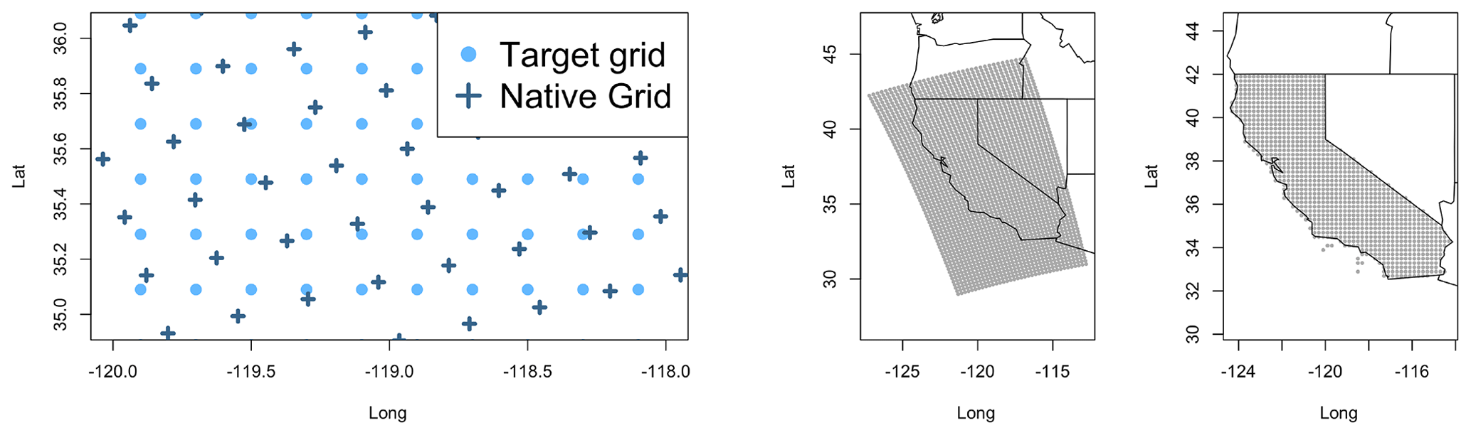
Figure 1A comparison of differing grid projections. The left shows a close up of two differing grids on a 20 km scale and a zoomed-out projection on the right.
We contrast the approach of just using the regridded RCM fields as the regression predictors with an empirical Bayesian model that explicitly incorporates the mismatch between the RCM grids and the NSRDB grid. The Bayesian approach takes advantage of recent tools in spatial statistics for conditional simulation of Gaussian processes and combines this with classical Bayesian formulas for linear regression (Cressie and Wikle, 2011). This strategy provides a simple framework to avoid the biases in an analysis based on a regridded estimate. Moreover, this method can be extended to more sophisticated prediction beyond a linear relationship. Our empirical Bayesian method uses the same spatial prediction model that would be used in standard regridding but adds a step to generate conditional samples of the spatial fields. These realizations then become the conditioned covariate in a Bayesian linear model, with a closed-form expression for sampling the posterior of the regression parameters. The Bayesian approach is useful for determining unbiased estimates of the regression parameters. However, if the goal is simply prediction based on the linear model, we also show that the standard regridding regression is appropriate for prediction, especially when prediction uncertainty is calibrated with a holdout sample. Therefore, how this problem is tackled depends partly on the end goals of the analysis.
We illustrate these ideas with an application to solar radiation prediction, and these results are important in their own right. The analysis suggests the limits of predictability of solar radiation based on regional climate model simulations and also points to how the models may be biased relative to the NSRDB data set.
The uncertainty in the regridding process for solar radiation has not been given much attention as it relates to climate simulations, but there are many studies of this issue for precipitation or temperature (Chandler et al., 2022; Rajulapati et al., 2021). McGinnis et al. (2010) considered regridding error for RCMs in four regridding methods – nearest neighbors, bilinear interpolation, inverse distance weights, and thin-plate splines for temperature and precipitation RCM data. The study found that thin-plate splines performed the best out of the four methods considered in terms of regridding but that the chosen interpolation method has a larger effect when considering local results as opposed to large-scale phenomena across multiple models. Additionally, spurious extrapolation results need to be considered, particularly when considering extreme events, which temperature and precipitation analyses often do. The need for regridding was bypassed in Harris et al. (2022), who proposed neural-network Gaussian process regression (NNGPR) for predicting temperature and precipitation reanalysis fields from the ECMWF Reanalysis v5. The proposed method simultaneously downscales the same variables to RCM spatial levels using NA-CORDEX (North American Coordinated Regional Climate Downscaling Experiment) RCM data for validation. The method defines the downscaling pixel by pixel for the output grid by averaging the input climate model fields and defining a Gaussian process between the climate model fields and the prediction point in the reanalysis field. Preliminary results from this study show marginal improvements over existing methods, including linear models, in terms of combining climate models and poor uncertainty quantification skill, which is a direct focus of this study. Additionally, there are minimal metrics for uncertainty quantification of the method. While our method does not simultaneously downscale solar radiation data, this will be addressed in future work, and the methods proposed in Harris et al. (2022) could be used for a comparative analysis.
The effects of regridding on precipitation statistics have also been widely studied (Accadia et al., 2003; Berndt and Haberlandt, 2018; Ensor and Robeson, 2008; Diaconescu et al., 2015; Rauscher et al., 2010). In particular, the effects from regridding were found to have the largest impact at higher quantiles (Rajulapati et al., 2021). The same study also found that the difference in precipitation statistics between the original and regridded data decreased with higher grid resolutions and vice-versa for lower resolutions. This is also true at fine temporal scales (i.e., daily, sub-daily).
Our understanding is that there is a gap in the literature in terms of analyzing the downstream effects on modeling after regridding and for solar radiation data in particular. Note that this focus is related to the classic errors in variable models (Whittemore, 1989), where covariates are unknown or contain problematic data. Predictions based on the covariates containing errors are reliable provided data with the errors are consistently used. However, inferring scientific relationships between the predictand and predictors is not reliable. Thus the focus in this study is whether final conclusions based on downstream modeling and evaluation of an RCM contribution to prediction skill will change when regridding uncertainty is taken into account. As noted above, this study includes an analysis of possible effects using a Bayesian regression approach in order to quantify the uncertainty due to regridding. In particular, we develop a Bayesian hierarchical model (BHM) as a complete description of the analysis uncertainties and then explain how simpler approaches result from approximations to this BHM (Cressie and Wikle, 2011). Although we do not showcase a complete Bayesian analysis, we believe our approximate version is informative and is more easily implemented than the full Bayesian posterior computations.
The rest of the article is organized as follows: Sect. 2 introduces and describes the data utilized in this article, followed by an overview of the BHM in Sect. 3; Sect. 4 details the method to analyze the uncertainty of regridding; Sect. 5 shows results from this analysis; and finally, Sect. 6 concludes this work and discusses future directions.
2.1 National Solar Radiation Database
Modeled solar radiation data are part of the NSRDB, provided by the National Renewable Energy Lab (NREL) (see Sengupta et al., 2018, and the references therein for more details). The NSRDB is widely used by a variety of agencies, including local and federal governments, utility companies, and universities. Although primarily used for energy-related applications, its uses have been extended to others such as the connection between solar exposure and cancer. The NSRDB contains hourly and half-hourly measurements for the three most common solar radiation variables: global horizontal irradiance (GHI), direct normal irradiance (DNI), and diffuse horizontal radiation (DHI) (in units of Wm−2). Solar radiation data are calculated using the Physical Solar Model, which takes as input satellite measurements, cloud properties, and GHI derived from DNI and DHI. The data product for GHI and DNI has been validated and shown to be within 5 % and 10 %, respectively, when compared to surface observations. The NSRDB covers all of North America and surrounding countries for the years 1998–2021 at a 4 km resolution. For the purposes of this study, however, the data set is averaged to a grid resolution of 20 km to be comparable with climate model outputs at a similar resolution. The reader may note that the step of aggregation is related to the change-of-support problem (Cressie, 1996; Gelfand et al., 2001). In aggregating from the 4 to the 20 km grid for the NSRDB data set, we are hoping to avoid the change-of-support issue and to target the problem of regridding rather than the problem of downscaling. By using data that are on the 20 km grid for the NSRDB, which closely aligns to the size of the RCM grid, we are isolating the problem of regridding, and we target the uncertainty related to this step only.
2.2 Climate model database
Climate model data are sourced from the NA-CORDEX data archive, containing RCM output forced by various global climate models (GCMs) (McGinnis and Mearns, 2021; Mearns et al., 2017). The NA-CORDEX data archive contains many common climate variables, including surface downwelling shortwave radiation, at daily scales and sub-daily scales for some variables. Note that surface downwelling shortwave radiation is recorded as “rsds” in NA-CORDEX but is equivalent to GHI and is measured in the same units. Therefore, it will be referred to as GHI throughout this article. The archive includes ERA-Interim-driven runs generally covering 1979–2014. GCM-driven runs cover both historical periods (1949–2005) and future years (2006–2100) for various climate path scenarios and a model domain covering all of the conterminous United States, as well as most of Alaska, Canada, Mexico, and the Caribbean.
The data chosen for this study will later be used in statistical downscaling operations for solar radiation for future years, and RCMs for this study are chosen with this long-term goal in mind. The outputs chosen for this study are three ERA-Interim-driven RCMs: the Weather Research and Forecasting model (WRF), the Canadian Regional Climate Model 4 (CanRCM4), and the fifth-generation Canadian Regional Climate Model from the University of Quebec at Montreal (CRCM5-UQAM). These RCMs have desirable representative concentration pathways (RCPs) and grid resolutions for future GCM-driven runs.
A key part of this study is understanding the predictability of solar radiation based on RCM simulations. Here we organize the statistical assumptions as a BHM for clarity. This helps in tracing the Bayesian approximation used in our application, and the standard approach based on regridding also follows as an additional approximation.
Let {si} be the NSRDB grid, and let y(si,t) denote the average daily solar radiation reported at grid point si and day t. For convenience, consider a single grid location and let denote the vector of all daily values at location si. In a similar way let xk(si,t) be the covariate value from the kth RCM at location si and day t. The key assumption here is that this covariate makes sense at locations that are not part of the native grid of the RCM, and so we define the correct covariate vector . With this assumption our main focus is on the linear model given below, applied to available days and for each target grid location:
where yi represents the observed data from the NSRDB at the ith location, Xi is an (M+1) column matrix formed from the constant term, M refers to the number of RCM covariates, and S is the matrix of seasonal covariates. We will also assume εi to be the mean zero multivariate normal and variance σ2. The estimated coefficients are the relative adjustments in matching the RCM simulations to observations. Overall the goal is to estimate the coefficients β and γ and to use these in a prediction model for unobserved yi. Of course this would be a straightforward problem in linear regression if Xi was known. However, the complicating issue is that Xi must be inferred from other locations of the RCM grid. Moreover, we also note the complication that εi may exhibit dependence over time, which makes it more difficult to derive valid measures of uncertainty. This will be discussed in Sect. 3.3. The values of εi will not show dependence over space but may show correlation at differing locations (). As we are running this model from climate model reanalysis data, the spatial correlation of the errors should naturally be accounted for when .
3.1 Observation and process levels
We assume a stationary Gaussian process model for transformed RCM fields that are independent over time. Let {uj} denote the native grid for the RCM simulated fields, distinct in the number and position from the NSRDB grid. The raw RCM solar variable, x, is transformed to x* with the log-linear function according to
for a fixed value of ν. We found this transformation makes a Gaussian process assumption on more reasonable and constrains predictions transformed back into the original scale to be positive. For x>ν, Γ(x) reverts to a linear transformation and so retains interpretability for the larger and more relevant solar values. In this study, ν is set to be the 20th percentile of the RCM values. The value of ν was chosen from a range of possible percentiles, spanning [10th, 50th], as it resulted in summary statistics for the regridded values that were closest to the same statistics calculated from RCM data on the native grid. In this way, the regridded values are as similar as possible using the ν=20th percentile compared to if a different value had been chosen.
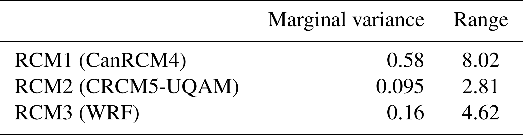
Given these transformed fields, we assume that, for fixed t, will be a Gaussian process with a mean function μk(s)=𝔼[xk(s)] and a stationary, exponential covariance function of
and for ,
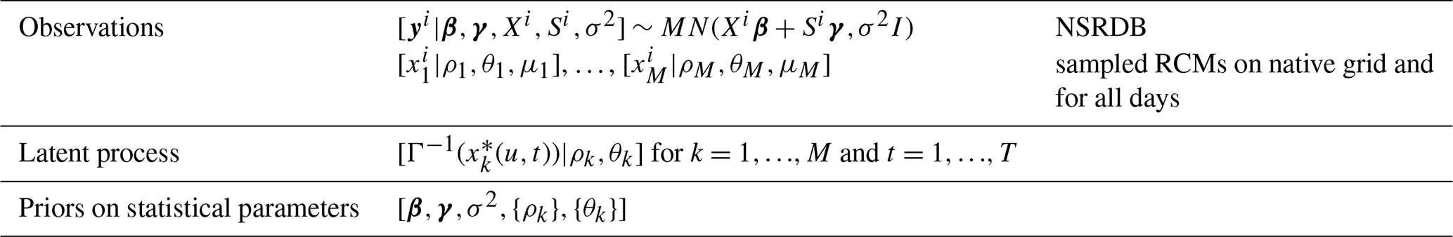
That is, we are assuming no temporal correlation in this process. However, we will relax this assumption in Sect. 3.3. Finally, in the following, it is convenient to let denote the kth RCM values on its native grid and for day t. With this setup, we have the BHM defined in Table 1. Here the latent processes are independent Gaussian processes with covariance given in Eq. (2). The joint distribution for this problem is thus
where yi, Si, and up to are the terms based on observed data that are fixed in the Bayesian computation. The Bayesian formalism is to identify this expression via Bayes theorem as proportional to the posterior density for the unknown parameters. Conceptually one would integrate this expression over to give a marginal posterior density in the statistical parameters. An exact integration, however, does not have a closed form, and instead, the standard approach is to sample from the posterior using Monte Carlo methods.
Table 1BHM for including regridding uncertainty into the coefficient estimates for multi-model analysis.
3.2 Approximate BHM
From a Bayesian perspective, this posterior is a complete characterization of the uncertainty in all unknown quantities. Unfortunately, in this case, as in many BHMs, there is not a closed form for the normalized posterior, and so one approximates this distribution. In our case a complete sampling of the posterior is complicated by the fact that the posterior for the Gaussian process covariance parameters is coupled to the linear model through the RCM covariates. Because the linear model only depends on the RCM through its value at the observation grid, one can break the sampling into two obvious steps and, in so doing, arrive at the usual strategy used for regridding.
- Step 1
-
Bayesian regridding. Sample from the density proportional to
- Step 2
-
Bayesian linear model. Sample from the density proportional to
The first step has been studied by several authors (Handcock and Stein, 1993; Finley et al., 2013) and is implemented with publicly available software and approximations for larger numbers of locations. This step can be approximated further by an empirical Bayes assumption where the maximum likelihood estimates (MLEs) for ρk, θk, and μk are substituted into the conditional distribution. Explicitly this approximation leads one to sample from a multivariate normal distribution:
Here, is the conditional mean for the RCM field on the target grid given the values on the native grid and given the covariate parameters at the MLE. is interpreted as the conditional covariance matrix describing the variation for the target grid values conditional on the native grid ones. Sampling from this distribution for fixed covariance parameters is referred to as conditional simulation in geostatistics, and several computational algorithms have been developed for large problems. We also note that the conditional mean vector, , in this setting is the well-known kriging spatial prediction from geostatistics. Finally, in this step, if one skips any sampling and sets , then this is the standard practice for regridding.
Several regridding methods were considered for this study, including thin-plate splines and bilinear interpolation. The chosen method, kriging with an exponential covariance function, performed the best when considering mean-squared errors on test data. Because this study is focused on the uncertainty in this step itself and, more importantly, the downstream effects of the regridding step, a single regridding method was chosen. The differences between regridding and interpolation methods themselves are considered in other studies (McGinnis et al., 2010).
The second step, conditional on having Xi in hand, is a standard Bayesian linear model. In our case, although not necessary, we adopt a noninformative, uniform prior on β,γ, and log (σ2), written as follows:
giving a posterior of
For the first term,
where and are the ordinary least-squares point estimates for the parameters, and
The marginal posterior distribution for σ2 is taken from the inverse Chi-square distribution:
where s2 is the unbiased variance estimate, also from ordinary least squares. The resulting posterior distributions for β and σ2 can then be compared to the linear model estimates for each location from Eq. (1). As a final approximation, the Bayesian computation can be made more efficient by omitting the posterior uncertainty in σ2 and substituting the point estimate into the first conditional density.
In summary, starting with a general formulation of predicting a field based on misregistered spatial covariates, we have detailed the series of approximations to identify the regridding algorithm. Here the RCM covariables are found by geostatistical prediction and substituted for the unknown fields values. The problem with this approach is highlighted by the matrix Ω−1 in Eq. (4), which determines and its uncertainty and is a nonlinear function of Xi. Thus substitution of a conditional mean of Xi into this expression will not be equivalent to the better approximation afforded by the sampling in step 2 above. In particular, is a nonlinear function of Xi. The conditional mean of the matrix inverse is not the same as substituting the conditional mean for Xi, and this difference suggests the BHM is the correct approach for quantifying the uncertainty calculated from Ω(⋅).
3.3 Autoregression component of BHM
It is worth mentioning that, in the above analysis, there is no time series addition to explain possible autocorrelation in the residuals. However, we determined that a temporal component may not be necessary through fitting several auto-regressive moving average models of order p and q (i.e., ARMA(p,q)) and assessing the resulting Akaike information criterion (AIC) and Bayesian information criterion (BIC) values. Across the 4 months considered (February, May, August, November), ARMA(0,0) was largely the best model according to both AIC and BIC. However, in August, an MA(2) model had the lowest AIC. Across all months, the model with the second lowest AIC or BIC was frequently an MA(2) or MA(1), followed by an AR(1) model. Although not crucial to our case study, for completeness, we have included below how the analysis would change with the addition of a time series component for the Bayesian analysis.
With a time series component for εi in Eq. (1), the final prediction results will be similar to those from the model in the previous section, but the prediction variance will be affected by the inclusion of an ARMA(p,q) model. Since single-parameter models (i.e., AR(p) or MA(q)) had lower AIC and BIC more frequently than higher-order models (i.e., ARMA(p,q)), the time series parameter for both MA and AR models will be denoted generically by η in the following.
The joint posterior in Eq. (3) becomes
Then, the joint density conditional on all parameters is
where now, the covariance matrix σ2Ω(η) depends on the autocorrelation parameter(s) η. This is useful for single-parameter time series models, such as AR(1) or MA(1), as well higher-order models ARMA(p,q) that are also causal and therefore can be written in an MA(∞) representation:
and it can be shown that the MA(∞) process has the autocovariance function
with the parameters depending on p and q from the AR and MA processes, respectively.
We now find the marginal posterior for . This can be done by averaging over β,σ2:
After some algebra, remarkably has a closed form, found through this integration:
where is the residual sum of squares found by fitting the linear model to yi conditional on Xi. With the marginal posterior distribution for η readily available, one samples values of η and continues with the analysis as outlined previously. Section 3.2 can be carried out by transforming the data and response through multiplying by , converting to an ordinary least-squares problem.
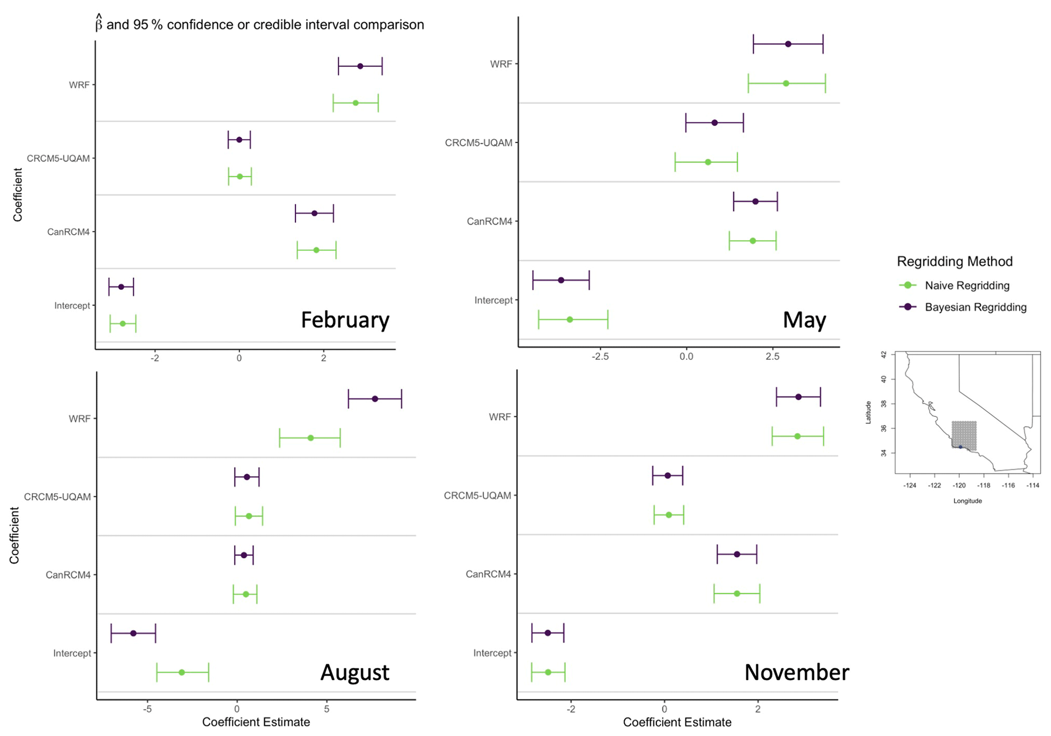
Figure 2Posterior predictions for each coefficient compared to the naive regridding estimates for a particular location in California for February, May, August, and November (1998–2009). The solid dots represent the point estimate for the naive regridding method and the median value of the posterior distribution from the Bayesian method. The whiskers represent the 95 % credible and confidence intervals for the posterior distribution and the naive regridding estimates, respectively.
The model described in Sect. 3 was fit once for each location in a subset area of California, shown in the far-right bottom panel of Fig. 2, which includes coastal and inland areas. Additionally, the model was fit for 4 separate months (February, May, August, and November) across all years of overlapping data (1998–2009). Initially, all covariates are included in the model. However, not all covariates were found to be significant. In particular, the CanRCM4.ERA-Int was found to hold no significance for the months of February, May, and November for most locations and no significance for about half of the locations in the month of August. The seasonal covariate held no significance for any of the months, which is expected since the data were subset into a single month from each season. Because of this, the seasonal covariate was removed for all 4 months.
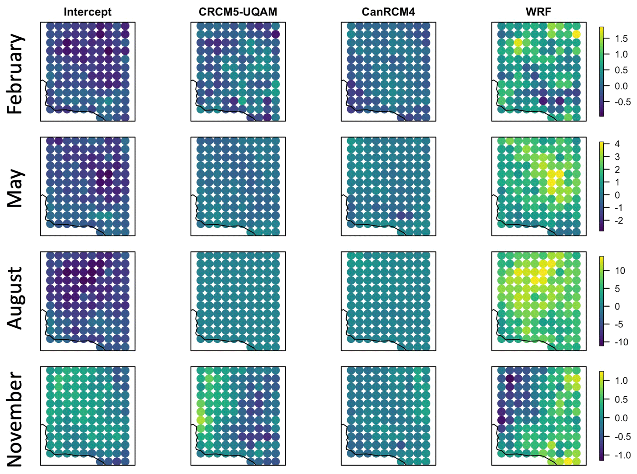
Figure 3Average bias by location between the naive regridding estimate and the median of all posterior distributions for February, May, August, and November, top to bottom, respectively.
4.1 Posterior distribution of model coefficients
Often, the regridded data set resulting from kriging is used as the ground truth for further analysis. This section outlines the method for analyzing the uncertainty associated with the regridding and linear model prediction step and downstream effects by generating draws from the posterior distributions of each β in Eq. (1).
The study design is as follows. For each RCM, 100 independent draws are made from the conditional distribution onto the NSRDB grid. This is step 1 outlined in Sect. 3.2. For each of these simulations, 50 draws from the posterior distribution for β and σ2 are taken, resulting in 5000 posterior draws. This is step 2 in Sect. 3.2. Since each conditional simulation is equally likely, the posterior draws are aggregated and summarized together. This is done for each of the 114 locations in the study subset. The 95 % credible intervals for the posterior distribution and the 95 % confidence interval for each are also considered. The 95 % credible intervals from the posterior distribution for the linear model parameters are determined by taking the 2.5 and 97.5 sample quantiles across the posterior samples.
4.2 Prediction coverage
This study also considers the coverage of the posterior predictions, i.e., the fraction of days where the prediction interval contains the actual value observed. This portion of the analysis holds out a single year of data as a testing set, using the remaining years as a training set. There are 12 years of overlapping data, resulting in 12 out-of-sample prediction results. The final coverage is the average coverage for the 12 folds.
The results presented here summarize the metrics outlined in Sect. 4. As the true coefficients are not known, we have supplemented the analysis with a simulation study. The design and results for this study are described in Appendix A.
5.1 Posterior distribution of model coefficients
Resulting parameter estimates from the posterior distribution vary by location and coefficient. Here we will refer to parameter bias as the difference between the naive estimate and that based on the Bayesian analysis. In general, the naive regridding model coefficient estimates are within the 95 % credible intervals of the posterior distributions for the respective coefficient. An example of the distributions compared to the naive regridding estimate can be seen in Fig. 2 for a location near the coastline of California across 4 different months. The green lines represent the naive regridding method, and the purple lines represent the Bayesian regridding method. In general, there is strong agreement between the two methods in both the point or median coefficient estimate, as well as in the confidence or credible intervals, suggesting that incorporating the uncertainty associated with the regridding step has little effect on model estimates. However, in the month of August (bottom-left plot), we see a case for the WRF coefficient where the methods do not agree and where this bias is offset by the intercept estimate. This bias in the WRF coefficient was seen across many locations for the month of August.
For the entire area considered, the average bias by location is shown in Fig. 3. The bias is calculated as the BHM estimate subtracted from the naive regridding estimate. Values close to zero indicate little difference between the two methods. Negative values indicate that the BHM gives a stronger weight to the model. The spatial patterns of the bias are most pronounced for the month of November and are also large for the month of August. In November, the average biases between the CRCM5-UQAM and WRF coefficient are spatially opposite in their signs but both hover around zero. Here, we can see that the naive method and BHM disagree most for the WRF coefficient in the month of August, with the naive method resulting in a much higher weight for WRF compared to the BHM. For additional reference, the estimated coefficient estimates and standard errors are provided in Appendix B.
5.2 Prediction coverage and error comparison
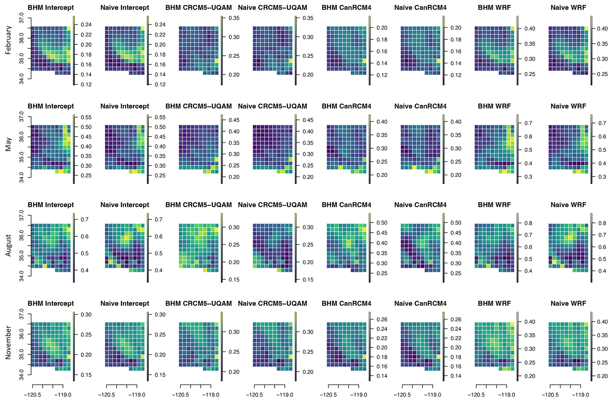
The prediction coverage of the naive regridding is calculated as the percentage of observations that are within the prediction intervals of the linear model. This is calculated by location for each of the 4 months considered. A similar method is implemented to calculate the coverage resulting from the BHM. We show results for the 4 months in Fig. 4. Note that, in the figure shown, the percent coverage reported is an average for holding out each year and is shown as the difference from the nominal level of 0.95. We see similar results for the out-of-sample coverage compared to the naive regridding.
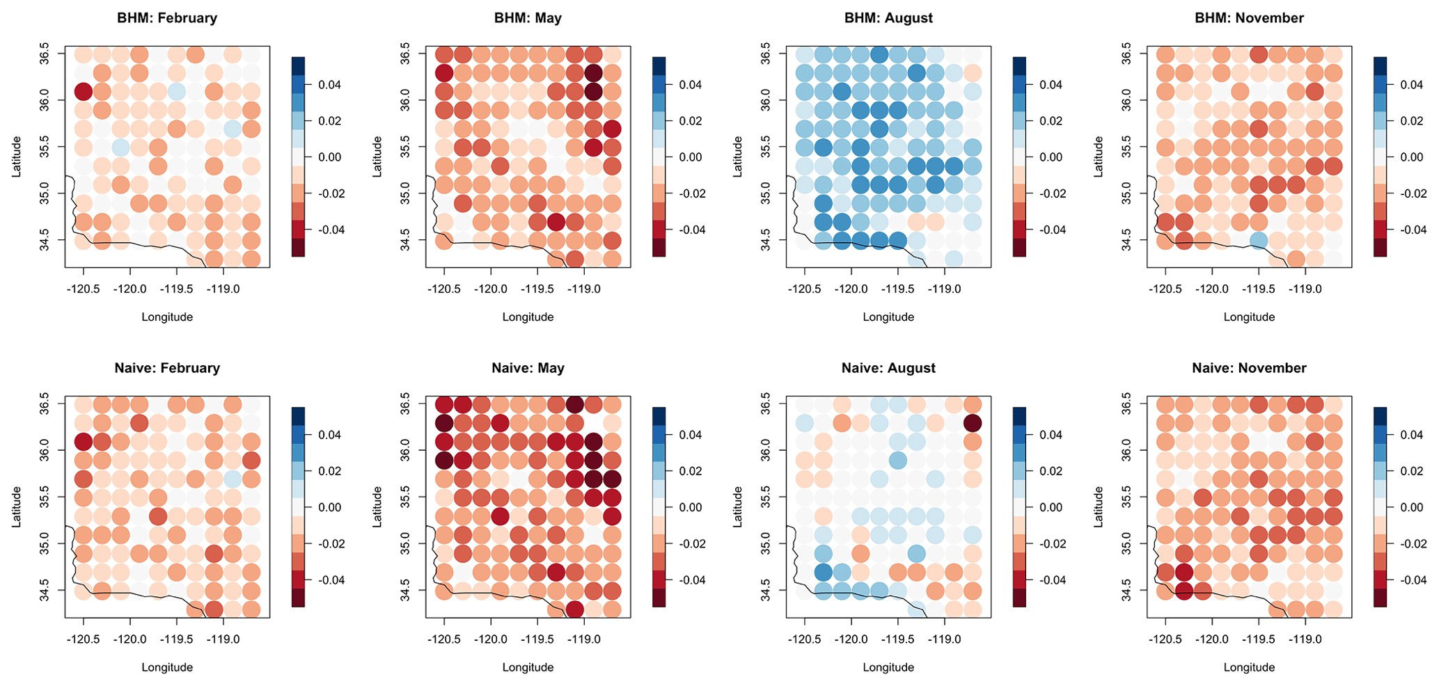
Figure 4Coverage probability shown as the difference from the nominal level (0.95) by location after holding out each year from 1998–2009 individually for the 4 months considered. Bayesian model results are in the top row, and naive regridding results are in the bottom row. Coverage is similar between the two models, hovering around 0.95, and is slightly higher in August.
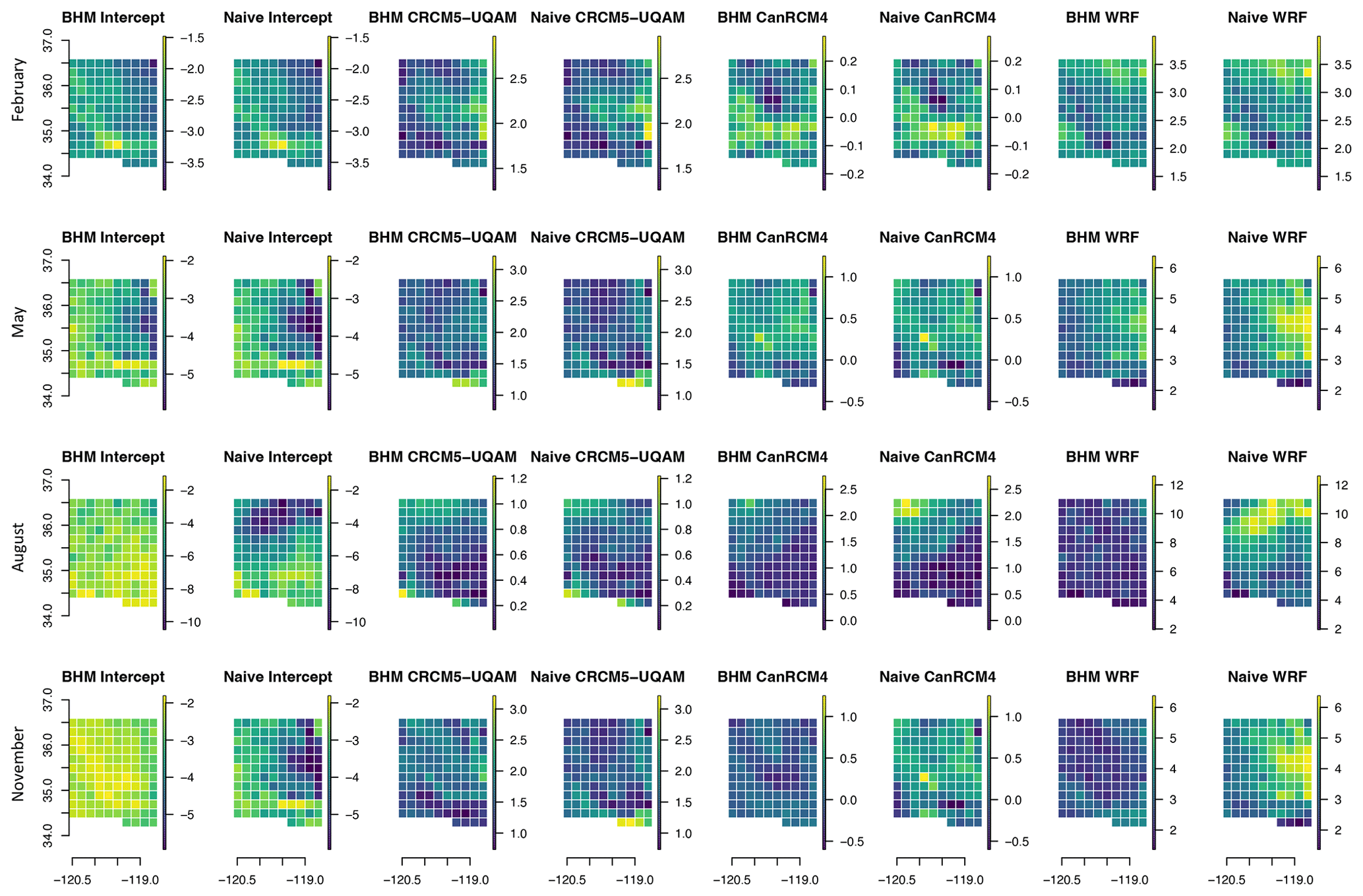
Similarly, the RMSE between the predicted GHI and the true GHI is lower across the study domain for August than it is for November in both the naive regridding model and the BHM, indicating better predictions for the summer month compared to the winter month. This is shown in Fig. 5. This finding may reflect a characteristic of seasonal solar radiation. Incoming solar radiation during summer months typically has a lower standard deviation when considered on a monthly or seasonal basis than in winter in California, indicating that there is less variability in day types (i.e., cloudy versus sunny) or in the amount of incoming solar radiation during the summer compared to the winter. Therefore, it makes sense that predictions have a lower RMSE in the summer months as the covariables and response have less variability during that season. The RMSE values are also lower for the naive regridding than they are for the BHM across the 4 months shown. When regridding uncertainty is taken into account, the predicted GHI values have a higher error than when prediction is done directly without considering regridding uncertainty. This is an interesting finding in that it suggests that doing prediction directly without considering any uncertainty may produce more accurate point predictions, but regridding uncertainty contributes additional variability to the final point estimates, as seen in the BHM.
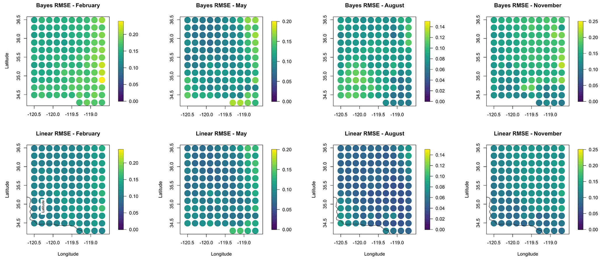
Figure 5A comparison of the RMSE values for out-of-sample prediction for the 4 months considered. Bayesian model results are in the top row, and naive regridding results are in the bottom row. The RMSE is generally higher for the Bayesian results and in November for both models.
This study analyzes the uncertainty in the regridding of spatial data from climate models, which is often the first step in multi-model climate analysis. Solar radiation data are regridded from their native grid, using kriging with an exponential covariance function and a log-linear transformation, to the same grid as the NSRDB. Second, we implement a BHM to estimate linear model weights while incorporating the uncertainty associated with the regridding step. Finally, we compare the two and provide an additional simulation study in Appendix A. The naive regridding model coefficient estimates were found to be within the range of the posterior distributions of the model coefficients in most cases. Seasonally, the month of August produced a mismatch between the naive regridding coefficient and the posterior distribution for the WRF RCM forced by ERA-Interim. In particular, we saw that the resulting coefficient estimates in this month for the WRF were higher in the naive method than the BHM. This suggests that, when regridding uncertainty is taken into account, there is a smaller increase in the WRF data for unit increases in the NSRDB or that the regridding uncertainty may result in less bias from the WRF in this particular case.
It was found that the posterior coverage for test data for the simulated fields was similar to the naive regridding estimates for the months of August and November. This suggests that, when taking into account the regridding uncertainty of the simulated fields and the model parameters themselves, the true value of solar radiation in this case is still likely to be covered by the 95 % credible interval. Therefore, if the conditional mean of the regridded field were taken for ground truth, as it often is, downstream effects of regridding on modeling appear to be minimal in the case of solar radiation. However, the BHM had higher RMSE values than the naive regridding models in the months considered, indicating that the addition of the regridding uncertainty increased prediction error for out-of-sample prediction. It is important to note that the naive regridding coefficient estimates give good predictions but are not appropriate to assess the model biases directly since model biases are dependent on regridding.
Finally, this analysis serves as a framework for understanding regridding effects within the context of solar radiation. While this study did not find situations where the BHM regridding consistently outperformed the naive regridding method, we note that this analysis revolves around the chosen variable: GHI. It has been shown that the chosen regridding method has an impact on the extremes of distributions (McGinnis et al., 2010); however, extremes are not central to solar radiation. A future analysis applying the BHM regridding method to climate variables where extremes of the data are more widely studied, such as precipitation or temperature, may yield different results and provide an example where the method proposed in this paper might show higher uncertainty in downstream modeling. Additionally, this study takes into account a single type of regridding (kriging with an exponential covariance), and this analysis could be extended to other types of interpolation to understand the downstream effects of those particular methods.
Here we implement a short simulation study which highlights some of the main differences, as well as similarities, between the naive method and the BHM.

Figure A1(a, b, c) Original RCM grid for the three RCMs used in the regridding study, plotted with NSRDB grid in blue. Magenta points represent the study area from the regridding study in the main text. (d, e, f) Subsetted grids used in the simulation study.
Table A1Covariance arguments used to simulate RCM data. All covariance functions are a Matérn with smoothness =1. No measurement error is included.
A1 Simulation study setup
For this simulation study, we utilize the same grids from the original regional climate models. The full grids used in the original study are shown in the top row of Fig. A1 with the RCM grids in gray and the NSRDB grid over California in blue. The magenta points represent the subsetted area used in the regridding study, which will be also be used in this short simulation study. The bottom row of Fig. A1 shows the grids used for this simulation study. The gray and blue dots show the true grids which include both the RCM and the NSRDB grid. The magenta points are again the simulation study area on the NSRDB grid. This will be explained more fully in the next section. We added a 2∘ buffer around the final study domain in magenta to avoid any edge effects in the simulation and regridding steps.
A2 Simulation study steps
The simulation study follows these steps:
-
Simulate ground truth data 100 times on the combined grids shown in Fig. A1. This is done using the Cholesky decomposition to result in an exact simulation of the Gaussian process given fixed covariance arguments. That is, for a fixed σ2 and θ, the process has the covariance function
for a distance d between two grid points. The covariance arguments that were estimated in fitting a spatial model to the RCM data for the month of August in the original study were again used here to create a realistic spatial process. This results in three sets of combined RCM and NSRDB data that follow the same defined GP. Each of the 100 fields represents a day of data. Since these days were assumed to be independent in our original study, we maintain this independence in the simulation here. The parameters used for each Gaussian process are in Table A1.
-
Subset the gray points in the bottom row of Fig. A1 to only the points that fall in the original RCM grid, in gray in the top row of Fig. A1. The true NSRDB observations are generated by weighting each RCM grid in a linear model by location:
where , and γi is fixed as the estimated variance of the residuals from the regridding study in the primary paper for the month of August. The estimated coefficients from the naive method for the same month from the original study are used here as weights for each RCM to create a realistic observation set on the magenta points or the NSRDB study area.
-
Regridding and model fitting are done for each method in the following way:
- a.
Bayesian regridding. Conditionally simulate each day or field 100 times onto the NSRDB study area from the RCM grids. For each simulation, run the BHM as described in Sect 3.2, and take 50 draws from the posterior distribution for each coefficient, resulting in a posterior distribution for each location and for each coefficient.
- b.
Naive regridding. Regrid once from the RCM grid to the NSRDB grid using kriging. Then estimate a linear model for each location across the 100 d, or fields.
- a.
-
Compare the coefficient estimates and standard errors of the coefficients from the naive regridding and the BHM regridding method.
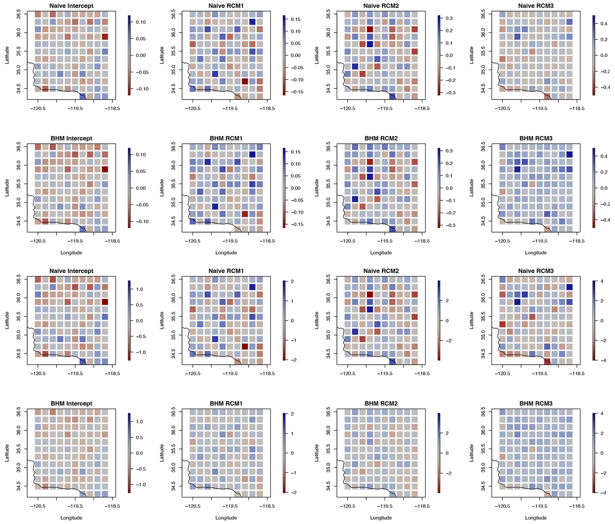
Figure A3Top: bias between the resulting coefficient estimates from the two methods and the true coefficients. Bottom: bias between the resulting coefficient estimates normalized by the RMSE between the true and estimated coefficients from each method.
A3 True coefficients
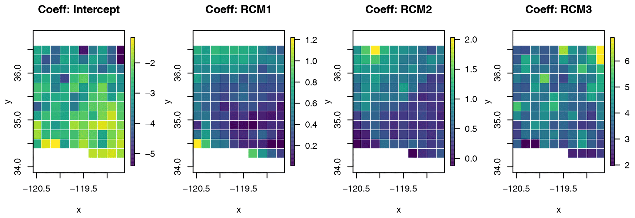
In step 2, the true response, representing the observations from the NSRDB, is generated by weighting each RCM at each location in the study area across all 100 d. These coefficients are set by taking the average from the BHM in the original study. The true values for the intercept and each RCM at each location are shown in Fig. A2. The weights correspond to the weights estimated for the CanRCM4, CRCM5-UQAM, and WRF. The WRF had the highest weight between the three RCMs in the original study.
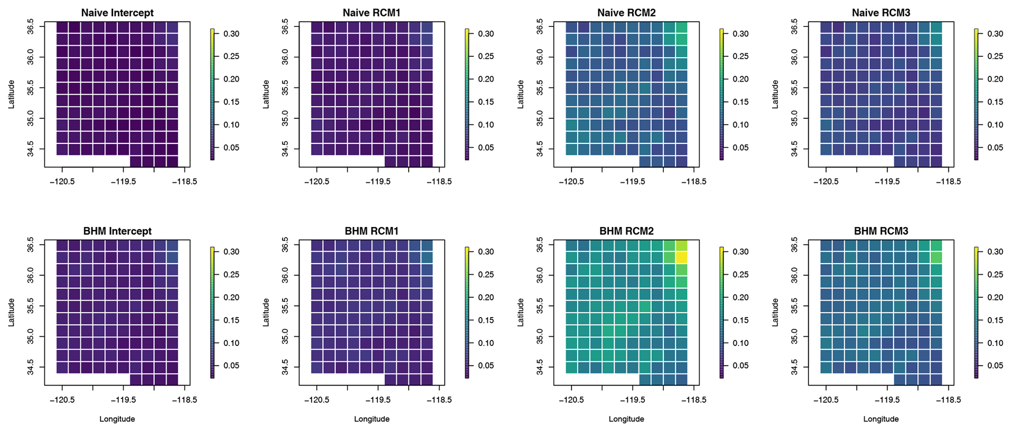
Figure A4Standard error of the estimated coefficients at each location in the simulation study area.
A4 Results
The raw differences relative to the RMSE between the estimated from the linear model and the mean of the posterior distribution for the BHM are shown in Fig. A3. Generally, relative to the overall variation of the error, the difference between the true and estimate coefficients is smaller for the BHM and higher for the naive method. This indicates that the regridding uncertainty decreases the raw error in the estimated weights. We also see that, for the largest weight (RCM3), the BHM slightly underestimates β3, but the naive method sees larger errors. In general we can say that the bias between the estimates from the BHM is lower than that of the naive regridding method.
We can also look that raw error without normalizing by the RMSE, seen in Fig. A3. This figure shows similar errors between the two methods compared to the true coefficients. The exception is seen in the coefficient estimate for RCM3, which is slightly overestimated by the BHM when considering the raw difference compared to the RCM, which slightly underestimates or is closer to the true coefficient.
One interesting finding is that the coefficient standard error is larger for the posterior distribution of the BHM estimates than it is for the naive coefficient estimates. This is seen in Fig. A4, where the top row shows the standard error for the naive regridding coefficient estimates, and the bottom row shows the posterior standard deviations of the BHM estimates. The coefficient standard error for the BHM estimates is, on average, 46 % larger than it is for the naive method. This signifies that incorporating the regridding uncertainty results in a slightly wider range of potential weights for the RCMs in predicting the observed values. However, the difference in the standard error is not large, and because the posterior mean of the BHM coefficient estimates and the naive regridding estimates are very similar, this result may not have much of an effect in this application.
A5 Simulation study conclusions
This simulation study highlights some important differences between the naive regridding and BHM regridding methods. In particular, the biases between the true coefficients (weights) and the estimated weights is smaller relative to the error variance for the BHM and larger for the naive method. This indicates that, when regridding uncertainty is taken into account, the BHM is more precise in estimating the RCM weights. This finding is further emphasized in the standard error of the coefficients for the two methods. This value is lower for the BHM than it is in the naive method, though the difference in standard error between the two methods is small. Overall we can conclude that taking regridding uncertainty into account results in more precise estimates for model weights when predicting observed values based on climate model output. This precision provides increased understanding in which climate model may have higher importance in predicting observed outcomes and, therefore, future projections for solar radiation.
All code producing results in this paper can be access through https://doi.org/10.5281/zenodo.10054998 (Bailey, 2023).
Data from the NSRDB can be accessed online through the NSRDB viewer, through the AWS cloud services, or through NREL's System Advisory Model (https://nsrdb.nrel.gov/, Sengupta et al., 2018). NA-CORDEX data can be accessed directly through https://doi.org/10.5065/D6SJ1JCH (Mearns et al., 2017).
MDB conducted all statistical analyses and wrote the paper; SB and DN contributed to the paper and advised on all statistical analyses; MS, AH, and YX provided expertise in the application to solar radiation.
At least one of the (co-)authors is a member of the editorial board of Advances in Statistical Climatology, Meteorology and Oceanography. The peer-review process was guided by an independent editor, and the authors also have no other competing interests to declare.
The views expressed in the article do not necessarily represent the views of the DOE or the U.S. Government.
Publisher’s note: Copernicus Publications remains neutral with regard to jurisdictional claims made in the text, published maps, institutional affiliations, or any other geographical representation in this paper. While Copernicus Publications makes every effort to include appropriate place names, the final responsibility lies with the authors.
This work was authored by the National Renewable Energy Laboratory, operated by Alliance for Sustainable Energy, LLC, for the US Department of Energy (DOE) under contract no. DE-AC36-08GO28308. The views expressed in the article do not necessarily represent the views of the DOE or the US Government. The US Government retains and the publisher, by accepting the article for publication, acknowledges that the US Government retains a nonexclusive, paid-up, irrevocable, worldwide license to publish or reproduce the published form of this work, or allow others to do so, for US Government purposes.
Funding was provided by the U.S. Department of Energy Office of Energy Efficiency and Renewable Energy Solar Energy Technologies Office.
This paper was edited by Robert Lund and reviewed by two anonymous referees.
Accadia, C., Mariani, S., Casaioli, M., Lavagnini, A., and Speranza, A.: Sensitivity of precipitation forecast skill scores to bilinear interpolation and a simple nearest-neighbor average method on high-resolution verification grids, Weather Forecast., 18, 918–932, 2003. a
Bailey, M.: Regridding Uncertainty for Statistical Downscaling of Solar Radiation. In Advances in Statistical Climatology, Meteorology, and Oceanography, Zenodo [code], https://doi.org/10.5281/zenodo.10054998, 2023. a
Berndt, C. and Haberlandt, U.: Spatial interpolation of climate variables in Northern Germany-Influence of temporal resolution and network density, J. Hydrol., 15, 184–202, 2018. a
Chandler, R., Barnes, C., Brierley, C., and Alegre, R.: Regridding and interpolation of climate data for impacts modelling – some cautionary notes, EGU General Assembly 2022, Vienna, Austria, 23–27 May 2022, EGU22-4004, https://doi.org/10.5194/egusphere-egu22-4004, 2022. a
Cressie, N. and Wikle, C. K.: Statistics for Spatio-Temporal Data, John Wiley & Sons, Wiley Series in Probability and Statistics, 624 pp., ISBN 978-0-471-69274-4, 2011. a, b
Cressie, N. A.: Change of support and the modifiable areal unit problem, Geographical Systems, 3, 159–180, 1996. a
Diaconescu, E. P., Gachon, P., and Laprise, R.: On the remapping procedure of daily precipitation statistics and indices used in regional climate model evaluation, J. Hydrometeorol., 16, 2301–2310, 2015. a
Ensor, L. A. and Robeson, S. M.: Statistical characteristics of daily precipitation: comparisons of gridded and point datasets, J. Appl. Meteorol. Clim., 47, 2468–2476, 2008. a
Finley, A. O., Banerjee, S., and Gelfand, A. E.: spBayes for large univariate and multivariate point-referenced spatio-temporal data models, arXiv [preprint], https://doi.org/10.48550/arXiv.1310.8192, 30 October 2013. a
Gelfand, A. E., Zhu, L., and Carlin, B. P.: On the change of support problem for spatio-temporal data, Biostatistics, 2, 31–45, 2001. a
Handcock, M. S. and Stein, M. L.: A Bayesian analysis of kriging, Technometrics, 35, 403–410, 1993. a
Harris, T., Li, B., and Sriver, R.: Multi-model Ensemble Analysis with Neural Network Gaussian Processes, arXiv [preprint], https://doi.org/10.48550/arXiv.2202.04152, 8 February 2022. a, b
Loghmari, I., Timoumi, Y., and Messadi, A.: Performance comparison of two global solar radiation models for spatial interpolation purposes, Renew. Sust. Energ. Rev., 82, 837–844, 2018. a
McGinnis, S. and Mearns, L.: Building a climate service for North America based on the NA-CORDEX data archive, Climate Services, 22, 100233, https://doi.org/10.1016/j.cliser.2021.100233, 2021. a
McGinnis, S., Mearns, L., and McDaniel, L.: Effects of Spatial Interpolation Algorithm Choice on Regional Climate Model Data Analysis, Fall Meeting, American Geophysical Union, San Francisco, 13–17 December 2010, GC43F-1016, 2010. a, b, c, d
Mearns, L. O., McGinnis, S., Korytina, D., Arritt, R., Biner, S., Bukovsky, M., Chang, H. I., Christensen, O., Herzmann, D., Jiao, Y., and Kharin, S.: The NA-CORDEX dataset, version 1.0, NCAR Climate Data Gateway, Boulder CO [data set], https://doi.org/10.5065/D6SJ1JCH, 2017. a, b
Phillips, D. L. and Marks, D. G.: Spatial uncertainty analysis: propagation of interpolation errors in spatially distributed models, Ecol. Model., 91, 213–229, 1996. a
Rajulapati, C. R., Papalexiou, S. M., Clark, M. P., and Pomeroy, J. W.: The perils of regridding: examples using a global precipitation dataset, J. Appl. Meteorol. Clim., 60, 1561–1573, 2021. a, b
Rauscher, S. A., Coppola, E., Piani, C., and Giorgi, F.: Resolution effects on regional climate model simulations of seasonal precipitation over Europe, Clim. Dynam., 35, 685–711, 2010. a
Sengupta, M., Xie, Y., Lopez, A., Habte, A., Maclaurin, G., and Shelby, J.: The national solar radiation data base (NSRDB), Renew. Sust. Energ. Rev., 89, 51–60, 2018 (data available at: https://nsrdb.nrel.gov/, last access: 2 Novemver 2018). a
Whittemore, A. S.: Errors-in-variables regression using Stein estimates, Am. Stat., 43, 226–228, 1989. a
- Abstract
- Copyright statement
- Introduction
- Data
- Bayesian hierarchical model (BHM)
- Solar radiation example
- Results
- Conclusions
- Appendix A: Simulation Study
- Appendix B: Regridding coefficient estimates
- Code availability
- Data availability
- Author contributions
- Competing interests
- Disclaimer
- Acknowledgements
- Financial support
- Review statement
- References