the Creative Commons Attribution 4.0 License.
the Creative Commons Attribution 4.0 License.
 | 05 Jun 2023
Statistical modeling of the space–time relation between wind and significant wave height
Said Obakrim
Pierre Ailliot
Valérie Monbet
Nicolas Raillard
Many marine activities, such as designing ocean structures and planning marine operations, require the characterization of sea-state climate. This study investigates the statistical relationship between wind and sea states, considering its spatiotemporal behavior. A transfer function is established between wind fields over the North Atlantic (predictors) and the significant wave height (predictand) at three locations: southwest of the French coast (Gironde), the English Channel, and the Gulf of Maine. The developed method considers both wind seas and swells by including local and global predictors. Using a fully data-driven approach, the global predictors' spatiotemporal structure is defined to account for the non-local and non-instantaneous relationship between wind and waves. Weather types are constructed using a regression-guided clustering method, and the resulting clusters correspond to different wave systems (swells and wind seas). Then, in each weather type, a penalized linear regression model is fitted between the predictor and the predictand. The validation analysis proves the models skill in predicting the significant wave height, with a root mean square error of approximately 0.3 m in the three considered locations. Additionally, the study discusses the physical insights underlying the proposed method.
- Article
(8588 KB) - Full-text XML
- BibTeX
- EndNote


A sea state is a statistical description of the sea surface waves generated by wind at a given time and location. The sea state is characterized by a superposition of wind seas and swells (Ardhuin and Orfila, 2018). The local wind generates wind seas, whereas swells are generated in distant areas. Significant wave height (Hs), defined as 4 times the zeroth moment of the wave power spectrum, is commonly used to describe the sea state. Thus, Hs is an essential measure of wave height and provides information about the wave energy of a given sea state.
High-quality wave data are essential for many marine applications, such as designing coastal and offshore structures and planning marine operations. Observational, numerical, and statistical models are the methods used for sea-state characterization. Traditional in situ measurements obtained from buoys provide the most reliable data for sea-state parameters; however, they are only available for the last decades and are limited spatially (Ardhuin et al., 2019). Numerical models (Hasselmann et al., 1973; Tolman, 2009) provide simulations of spectral wave models from which sea-state parameters are extracted. They are a valuable source of data and provide decades of records, although they are computationally expensive. Statistical models constitute an alternative to numerical models for constructing the wind–waves relationship. These models are not computationally expensive, and once the statistical relationship is estimated, future predictions can be made by assuming that this relationship is stationary, meaning that the statistical relationship between the large-scale variables and the sea-state parameters does not change between the present and the future (Mori et al., 2013; Laugel et al., 2014).
Various studies have compared statistical and numerical models for ocean wave parameters and other climate variables. Wang et al. (2010) compared these methods in terms of climatological characteristics of the present period using ERA-40 wave data. They found that the statistical models are better at reproducing the observed climate than the dynamical models. Laugel et al. (2014) analyzed these methods for climate projections, and their study shows that statistical downscaling (SD) approaches can reproduce the present climatology and future projections. In addition, due to their low computational complexity, SD models permit the consideration of a wide range of global climate models (GCMs) and climate scenarios, which allows us to estimate the uncertainties. However, modeling the relationship between wind and sea-state parameters using statistical methods still presents some difficulties, which have been addressed by different methods in the literature, namely:
-
Waves depend on both local and global wind conditions. The surface wind generates wind waves. However, it is not only the local wind that defines local waves, and wind from distant regions generates swells that may reach the target point (Ardhuin and Orfila, 2018). Therefore, SD models have to consider both wind sea and swells, which is particularly challenging in swell-dominated areas (Hemer et al., 2012). To address this issue, we use a local and a global predictor to account for wind sea and swells, respectively, as already done in Casas-Prat et al. (2014) and Camus et al. (2014a).
-
Wind conditions are multicollinear and multidimensional. The wind conditions are characterized by two components (zonal and meridional), which might be challenging to consider directly in a statistical model. To address the issue of multidimensionality in this study, we introduce the wind projection, which consists of retaining only the fraction of wind blowing towards the target point. The proposed preprocessing step allows the use of only one variable for each grid point, reducing the dimension of the predictor by half. Furthermore, large-scale wind variables are high-dimensional and multicollinear (strong correlations among variables) due to the strong spatiotemporal dependence of wind fields, and using them as a predictor in a statistical model might be challenging. Dimensionality-reduction methods such as principal component analysis are typically used as a preprocessing step to reduce the dimension of the large-scale variables and deal with multicollinearity (Laugel et al., 2014; Camus et al., 2014a, b). In this study, we use ridge regression (Hoerl and Kennard, 1970), which has been proven to be beneficial for dealing with multicollinearity in various studies (Mahajan et al., 1977; Hessami et al., 2008).
-
The relationship between wind and waves is not instantaneous. Wind from distant regions generates waves that may take days to reach the target point. Thus, the relationship between wind and waves is not instantaneous. Therefore, it is necessary to consider lagged wind conditions to understand the wave dynamics at a particular target location. The optimal lag at each grid point is interpreted as the travel time required for the waves to reach the target point (Camus et al., 2014a). ESTELA (Evaluation of Source and Travel-time of wave Energy reaching a Local Area) (Pérez et al., 2014) is a method that defines the wave generation area and wave travel time at any ocean location worldwide. Using its spectral information, the method selects the fraction of energy that travels to the target point from selected source points. The ESTELA method was used in various studies to define the temporal coverage of predictors used in SD (Camus et al., 2014a, 2016; Hegermiller et al., 2017; Anderson et al., 2019; Cagigal et al., 2020; Costa et al., 2020). The present study uses a statistical approach to define the wave generation area. It is based on estimating waves' travel time from each source to the target point (optimal lag) using the maximum correlation between the significant wave height and wind conditions. Therefore, this method is not computationally expensive, and only wind and Hs data at the target point are required, and unlike ESTELA, no spectral data are needed.
This study presents a statistical approach for estimating the relationship between wind conditions and ocean waves. The approach is based on weather types, which are constructed using a regression-guided clustering algorithm. These weather types are then used to link the space–time wind fields over the North Atlantic (predictors) and the significant wave height (predictand) at three locations: northwest and southwest of the French coast and the English Channel. Then, regression with ridge regularization is used to fit the relationship between wind conditions and significant wave height at each weather type. The proposed methodology considers wind sea and swells and provides additional information about the spatiotemporal relationship between wind and waves. The main contribution of this work is that it provides an entirely data-driven approach for estimating the travel time of waves from any source point to a target point, which is essential for the definition of predictors. To the best of our knowledge, the only other approach in the literature that can be used for this purpose is ESTELA (Pérez et al., 2014), which relies on directional spectra over the spatial domain of the wave generation. These spectra are not always accessible and can be computationally costly and demand high storage capacity. Our proposed approach, however, utilizes wind fields and significant wave height at the point of interest, which are more accessible and less computationally costly. Additionally, it allows for the processing of buoy data or data from models with limited spatial coverage, as it does not require the directional spectra over the wave generation domain. Furthermore, this study proposes a relatively interpretable model with a limited number of weather types and uses ridge regularization (van Wieringen, 2015). The regularization is used to make the parameters of the regression more interpretable and to improve the generalization capability of the model.
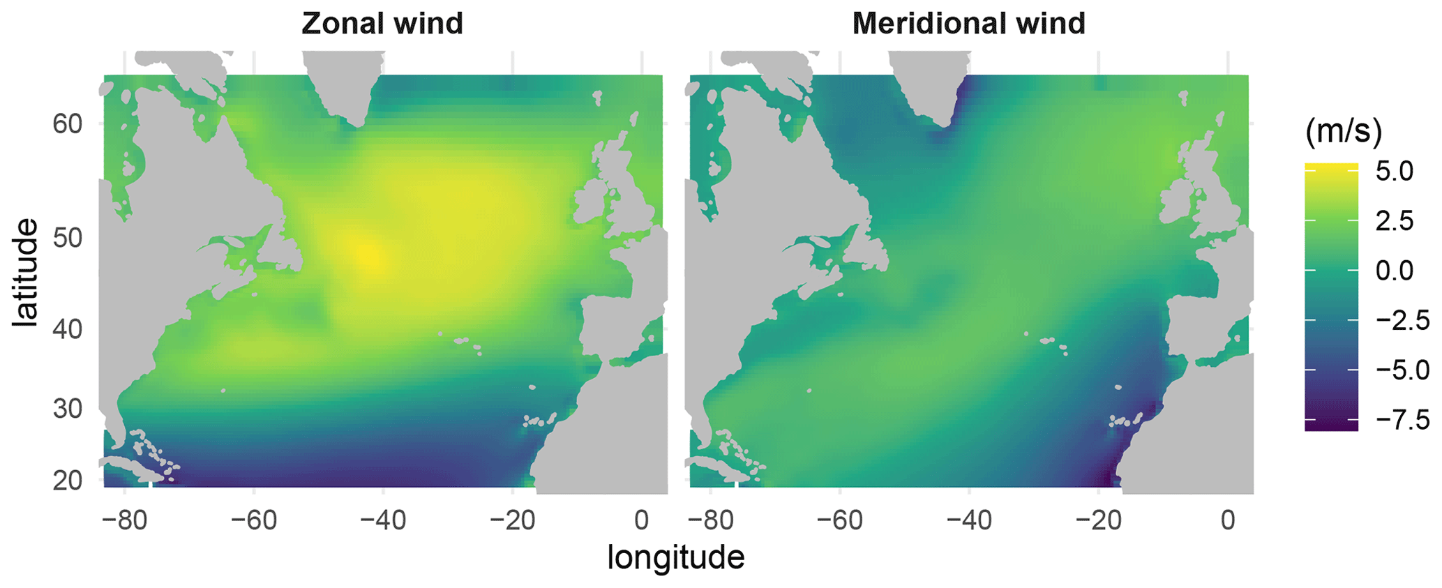
Figure 1Mean Climate Forecast System Reanalysis (CFSR) zonal and meridional wind components over the period 2014–2019.
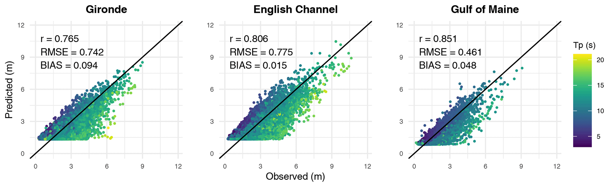
Figure 2Local model results (Eq. 1) in the validation period at the three considered locations as a function of the peak period (Tp).
This paper is structured as follows. After describing the data in Sect. 2, the local predictors are defined in Sect. 3. Then, Sect. 4 describes the construction of the global predictors. Next, Sect. 5 presents the statistical model that combines the local and global predictors. Then, Sect. 6 presents the results of the SD model. Finally, the study is concluded in Sect. 7.
The atmospheric data used in this work to construct predictors are extracted from the Climate Forecast System Reanalysis (CFSR) (Saha et al., 2010). CFSR is a global reanalysis developed at the National Centers for Environmental Prediction (NCEP) that covers the period from 1979 to the present with an hourly time step and spatial resolution of 0.5∘ by 0.5∘. Extracted data consist of hourly 10 m zonal and meridional wind components in the North Atlantic (Fig. 1).
To comprehensively evaluate the method across a range of observed sea states, we consider three different locations: Gironde (45.2∘ N, 1.6∘ W), the English Channel (49∘ N, 4.4∘ W), and the Gulf of Maine (43∘ N, 69∘ W). The Gironde location is nearshore, with the highest Hs observed at the considered period being 10.5 m, whereas in the English Channel location, which is offshore, the highest Hs observed is 11.8 m. In addition to the two eastern Atlantic locations, a location in the Gulf of Maine is situated in the western part of the Atlantic, where the maximum Hs reached 9 m. The bathymetry of the Gulf of Maine is highly complex, with a coastline dotted with numerous bays, islands, and coves (Panchang et al., 2008).
The historical wave data used in this work for the Gironde and English Channel locations are the sea-state hindcast database HOMERE (Boudière et al., 2013) based on the WAVEWATCH III® model forced by CFSR wind. The database covers the English Channel and the Bay of Biscay with unstructured computational mesh. It contains 37 parameters and the frequency spectra on high spatial resolution, ranging from 200 to 10 km, with a 1 h time step. For the Gulf of Maine location, we consider the IOWAGA database (Ardhuin et al., 2011), which is also based on the WAVEWATCH III® model forced by CFSR and ECMWF wind. To validate and interpret the results of the SD method, we consider the energy spectral partitioning, which identifies different wave systems. HOMERE uses the watershed algorithm (Tracy et al., 2007) to separate wind sea and different swells.
The temporal resolution of both predictors and predictand is upscaled from hourly to 3 h resolutions to facilitate the analysis. Both datasets comprise a common period of 26 years, from 1994 to 2019. The 1994–2013 period is used as the calibration period, while the 2014–2019 period is used as a validation period.
Wind speed, duration, and the fetch impact the characteristics of the wind sea (Ardhuin and Orfila, 2018). Hereafter, at time t, the variables U(t), F(t), U(t−1), and F(t−1) are considered to construct the local predictors. U(t) is the wind speed at the target point, and F(t) is the fetch length at time t, calculated as the minimum of the distance from the target point to shore in the direction from which the wind is blowing and 500 km. A minimum distance of 500 km is fixed because it is computationally expensive to calculate the distance between the target point and far away shores such as eastern American shores. Note that F(t) is not but is related to the fetch in the literature, which is defined as the distance over which waves develop (Ardhuin and Orfila, 2018). Lagged wind conditions are considered because they may provide information about the temporal variability of the wind and thus the duration of wind conditions.
To investigate the capability of local variables to explain Hs, the polynomial regression model,
is considered. Where X(ℓ) is the local predictor,
and β(ℓ) are model coefficients, and ϵ(ℓ)(t) is the model error. Model (1) contains polynomial terms and interactions between the fetch and squared wind to consider nonlinear relationships between Hs and predictors. We considered taking into account the lagged local wind conditions up to t−4; however, the performance of the model does not change as much as taking into account only the t and t−1 wind conditions.
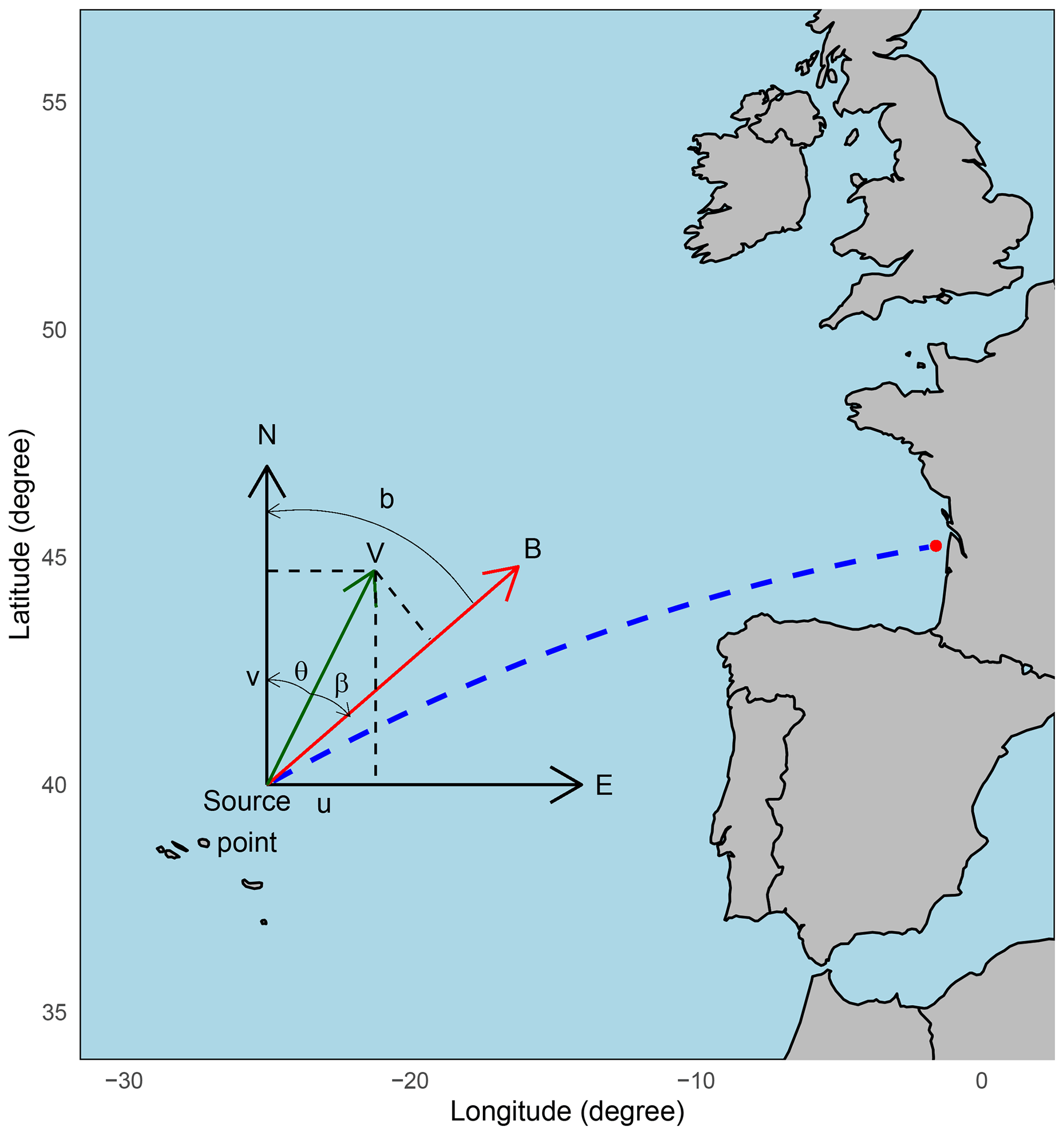
Figure 3Wind projection representation. The initial wind vector (V) at each source point is transformed into a component (B) aligned with the bearing (b) of the target point, as determined by a great circle path (dashed blue line).
The model is fitted using data from 1994 to 2013 and is assessed in a validation period from 2014 to 2019 using the Pearson correlation r, root mean square error (RMSE), and bias:
where is the predicted Hs at time t; and are the mean of observed and predicted Hs, respectively; and are the standard deviation of predicted and observed Hs, respectively; and n is the number of observations considered (58 440 for the calibration period and 17 528 for the validation period).
Results of the local model as a function of the peak period of the three considered locations are shown in Fig. 2. The model strongly underestimates high-period waves in all three locations and better predicts small-period waves. The high-period waves could correspond to swells that are generated far from the target point. Therefore, in order to predict Hs at these locations, it is important to consider the large-scale wind conditions that cover the swell generation as well as the local-scale wind conditions.
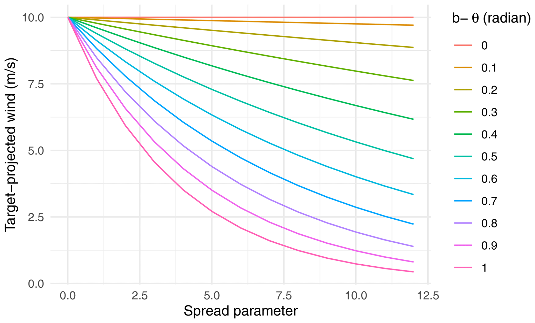
Figure 4Relationship between the target-projected wind and the spread parameter at varying values of the angle difference b−θ, with a constant wind speed (U=10 m s−1).
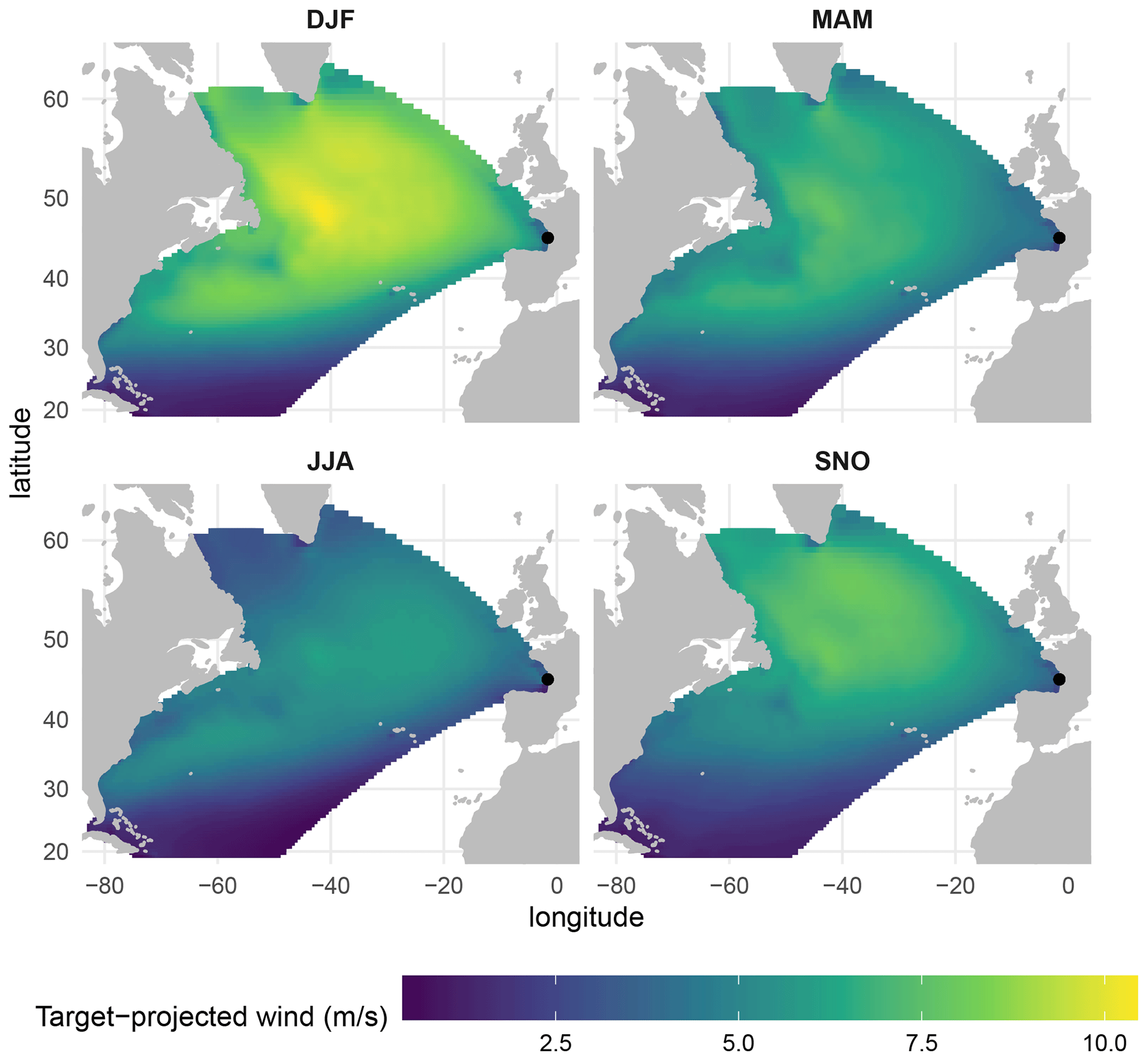
Figure 5Mean target-projected wind for Gironde in the winter (DJF), spring (MAM), summer (JJA), and autumn (SNO) over the period 2014–2019.
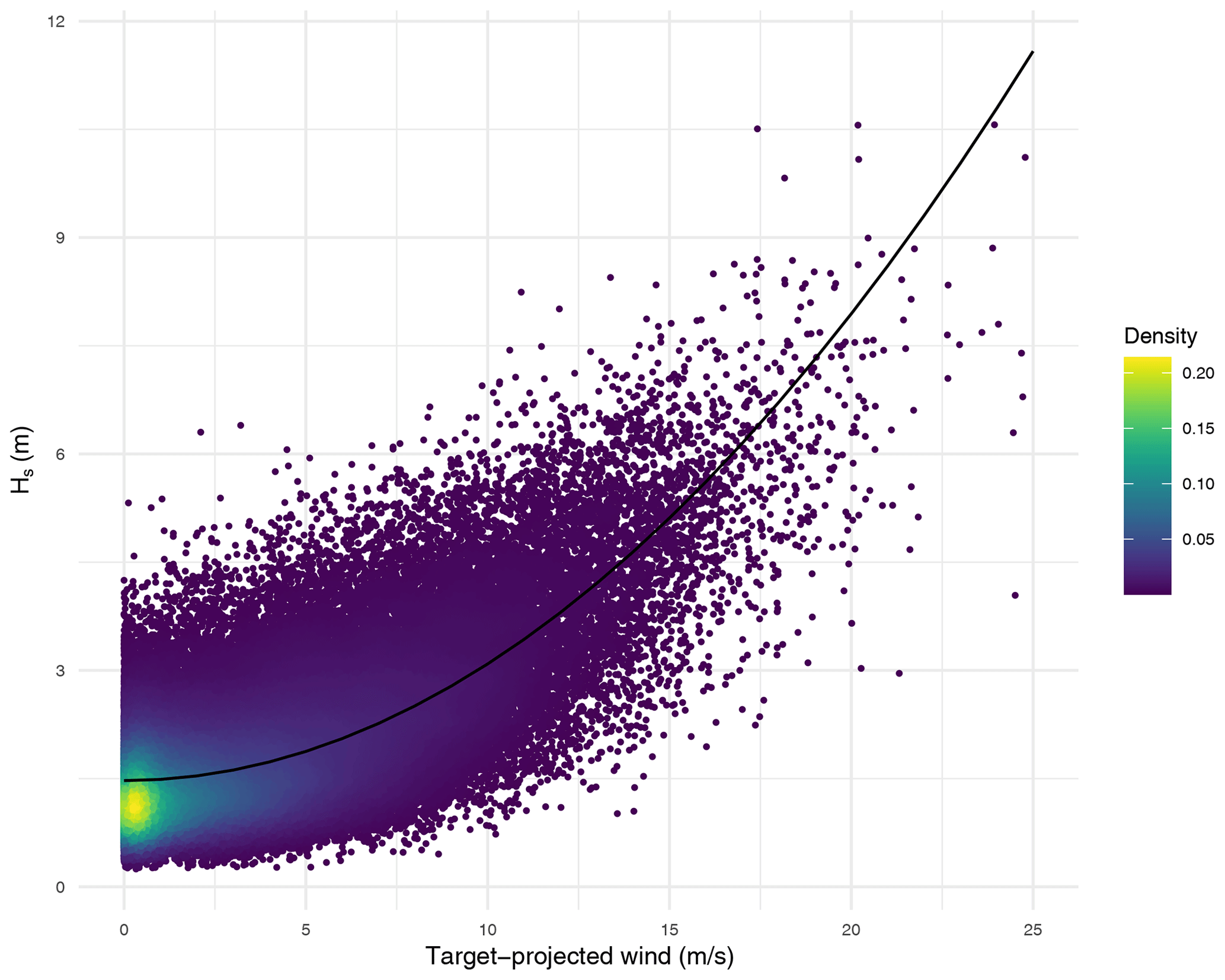
Figure 6Target-projected wind at point located in (45.5∘ N, 3.5∘ W) versus Hs and the estimated curve line using the model in Gironde.
In order to take swells into account, a global predictor which describes wind conditions over the North Atlantic has to be considered. Wind data have two components, the zonal and meridional components. Each of the two components in space and time carries more or less information about the waves observed at the target point at a given date. However, using all of them as inputs to a statistical model is computationally challenging, given the high dimensionality of the data and may lead to hardly interpretable results due to the strong correlation between wind conditions at closed locations in space and time. This section defines the global predictor related to the spatiotemporal domain of the wave generation area.
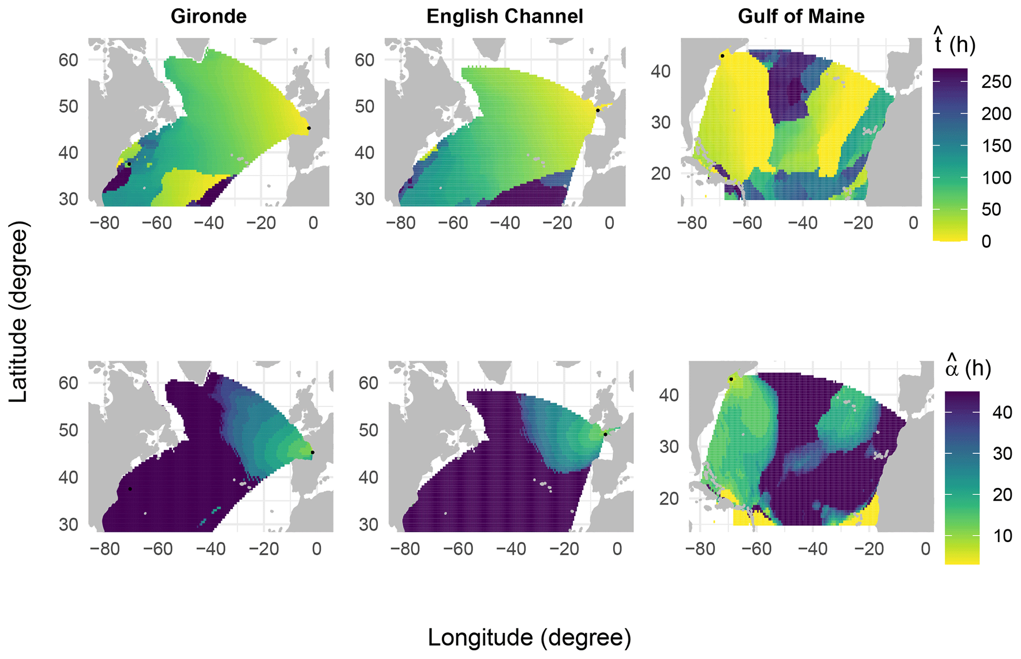
Figure 7Estimated travel time of waves (top panel) and the temporal width (bottom panel) using Eq. (9) in the three locations.
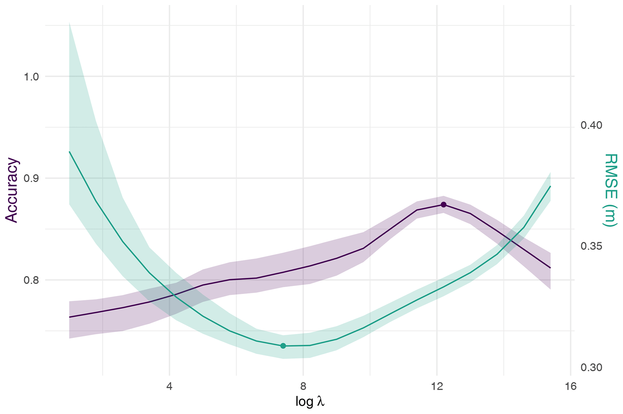
Figure 8Results of cross-validation using two weather types: RMSE (green line) and classification accuracy (purple line) versus the logarithm of λ. The red and blue dots correspond to the minimum RMSE and maximum accuracy, respectively. The interval for each criterion is defined as its minimum and maximum.
4.1 Spatial coverage
Following Pérez et al. (2014), the spatial coverage of the global predictor is based on the assumption that deep-water waves travel along a great circle path. Therefore, the wave generation area is limited by neglecting grid points whose paths are blocked by land. Furthermore, small islands are not taken into consideration.
4.2 Wind projection
To reduce the dimension of the atmospheric variables and to create a more interpretable model, wind components at each grid point are projected into the bearing of the target point in a great circle path (Fig. 3) using the following equation:
where W is the target-projected wind, U is the wind speed, s is the spread parameter (Young, 1999), b is the great circle bearing, and θ is the wind direction.
The parameter s≥0 controls the amount of wave energy being transferred by the wind blowing from different directions. In Fig. 4, the relationship between the target-projected wind and the spread parameter is examined at varying values of the angle difference b−θ, with a constant wind speed (U=10 m s−1). When the wind blows to the target point (i.e., θ≈b), the target-projected wind is near its maximum, which is the wind speed U. As the deviation of θ from b increases, the target-projected wind decreases, with the rate of decrease dependent on the value of the spread parameter. Therefore, a larger-spread parameter corresponds to less energy spreading. Ideally, s has to be smaller for locations near the target point and vice versa, and one can use an optimization method to select the optimal value for each location. To simplify the analysis and avoid the computation burden of such a method, we choose a common value of s for all locations. In order to evaluate the impact of the parameter s on the prediction of Hs, we tested a range of values for s between 0 and 7 using a simple linear regression model. The optimal value of s in terms of prediction accuracy was found to be 1 (not shown). Figure 5 illustrates the mean of the target-projected wind in the four seasons. Strong winds that blow towards the direction of the target point are observed in winter and mostly in the area around 50∘ N, 40∘ W.
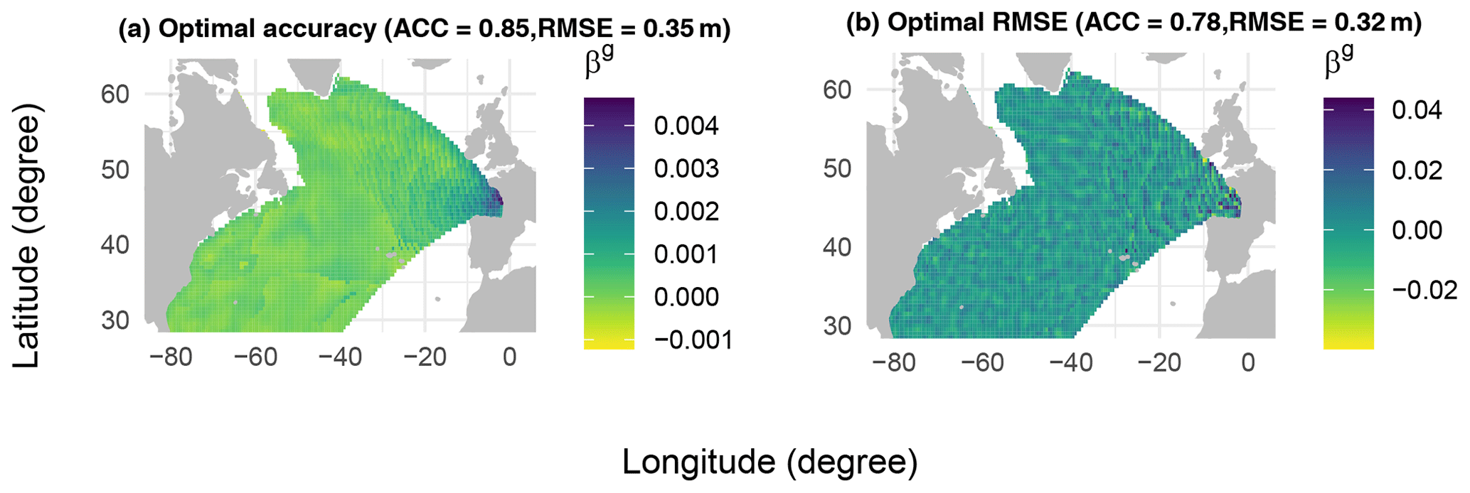
Figure 9Estimated global coefficients β(g) using ridge regression with λ that gives the maximum accuracy (a) and minimum RMSE (b).
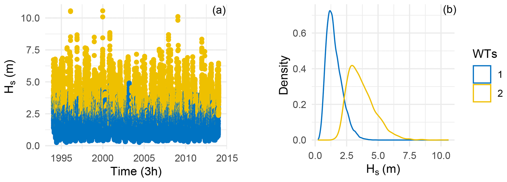
Figure 10Time series of Hs depending on the clusters (a) and empirical density (b) in the calibration period.
4.3 Temporal coverage
According to the dispersion relation, the group velocity of waves is expressed as
where g is the gravitational velocity and T is the period. For example, swells whose period is around 15 s have a group velocity of 11.73 m s−1, traveling 50 % faster than a 10 s ocean wave, and it takes them about 5 d to cross the Atlantic from Cape Hatteras to the Bay of Biscay (Ardhuin and Orfila, 2018). Therefore, waves generated at a location j and time t might take time tj to arrive at the target point.
At each location j and time t, the predictor is defined as the mean of the squared lagged target-projected wind in a time window so that
where αj controls the length of the time window, tj is the mean travel time of waves, Wj is the target-projected wind at location j, and n is the total number of observations. Henceforth, the parameter αj is called the temporal width, even though the length of the temporal wind is equal to 2αj+1. Note that the relationship between the target-projected wind and Hs seems to be a square relationship (Fig. 6) so that, in Eq. (8), the squared target-projected wind is considered.
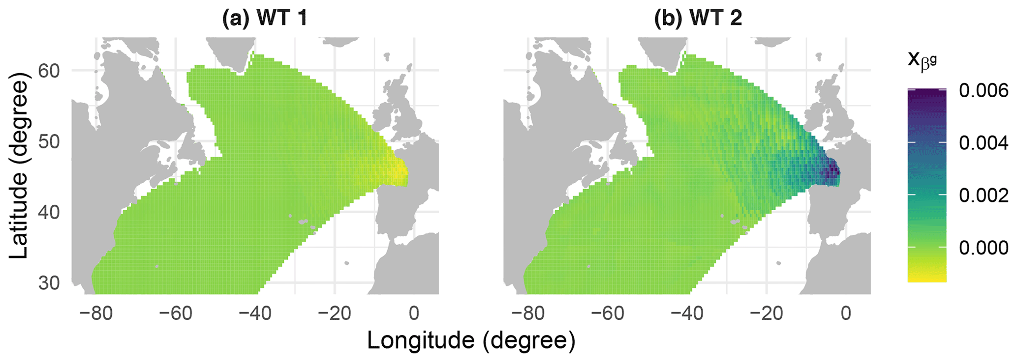
Figure 11Mean of minus the global mean for the cluster 1 (a) and cluster 2 (b).
The parameters tj and αj can be simultaneously determined for all locations by minimizing an objective function, such as least squares. However, this method is computationally infeasible due to its non-polynomial and combinatorial nature. As an alternative, tj and αj are independently estimated for each location over the entire period using the maximum Pearson correlation between the global predictor and Hs. At first, at each location j, the travel time tj is estimated by setting αj=0, then the temporal width is estimated using the estimated value of tj so that,
Figure 7 shows the estimated travel time of waves and the temporal width in the three locations. Globally, the two parameters are spatially smooth and interpretable, and as expected, the two parameters increase as the distance between the source and target point increases. For example, under the assumption of constant group wave velocity from the source to the target point, waves generated at a source point situated at 37.5∘ N, 70.5∘ W, which is 5642 km from the target point in Gironde, can take on average 180 h (about 7.5 d) to reach this target point. These waves travel at a velocity of 8.7 m s−1; thus, according to the dispersion Eq. (7), they have an average period of 11.1 s. On the one hand, considering as the maximum travel time of the waves, at the same source point, waves can also take 225 h (about 9 d) to reach this target point, with a velocity of 7 m s−1 and a period of 9 s. On the other hand, the minimum wave travel time () at the same source point is 135 h (about 5.5 d) with a velocity of 11.6 m s−1 and a period of 14.8 s. Therefore, tj−αj and tj+αj can be interpreted as the propagation time of long-period and short-period waves, respectively.
Regions located 35∘ S latitude exhibit inconsistent values of travel time. This may be attributed to the weak correlations between target-projected wind and Hs at the target locations. In such a situation, the optimal travel time value given by Eq. (9) may be very sensitive to the sampling error. Note that due to computational constraints, a maximum temporal width of 45 h was imposed in Eq. (9), and this constraint is visible on the bottom plots of Fig. 7.
5.1 Linear regression model
After defining the predictors, this section presents the statistical downscaling model. Firstly, the linear model that combines the local and the global predictor is considered:
where β(ℓ) and β(g) are local coefficients and global coefficients, respectively. Here β(ℓ) is not necessarily the same as in Eq. (1). is the local predictor defined in Eq. (2), is the global predictor defined in Eq. (8), and ϵ(t) is the model error.
5.2 Model fitting
Model (10) can be fitted using the least squares method; given by
where and . The least squares estimates in Eq. (11) are the best linear unbiased estimates of the parameters. However, since the global predictor is high dimensional (e.g., 67 108×5651 matrix for Gironde) and its variables are highly correlated, the matrix XTX may be ill-conditioned. Thus, the least squares estimates become highly sensitive to Hs variations. To address this issue, ridge regression (Hoerl and Kennard, 1970) minimizes the penalized residual sum of squares:
where λ≥0 is the regularization parameter. Note that the regularization is not applied to the parameters associated with the local predictor. The parameter λ allows us to take into consideration the bias–variance tradeoff.
5.3 Regression-guided clustering
Using the global predictor to construct weather types leads to clusters that only account for the global atmospheric circulation and not for the local environment (not shown). This subsection describes a regression-guided clustering method that considers both the global predictor and the predictand.
After estimating the coefficients, the contribution of a source point j at time t to Hs at the target point is defined as . The matrix of contributions is defined as
We expect swell systems coming from contributions from distant areas, whereas wind sea will be associated with local contributions. A natural question that arises is whether we can identify these wave systems by using . Subsequently, the k-means clustering algorithm is used on to obtain the weather types (WTs). Finally, the link function can be constructed by fitting each class's linear regression model (10). Therefore, model (10) now becomes
where and are local and global coefficients for the class k. Ik denotes all time indices that are in class k, and K is the total number of WTs.
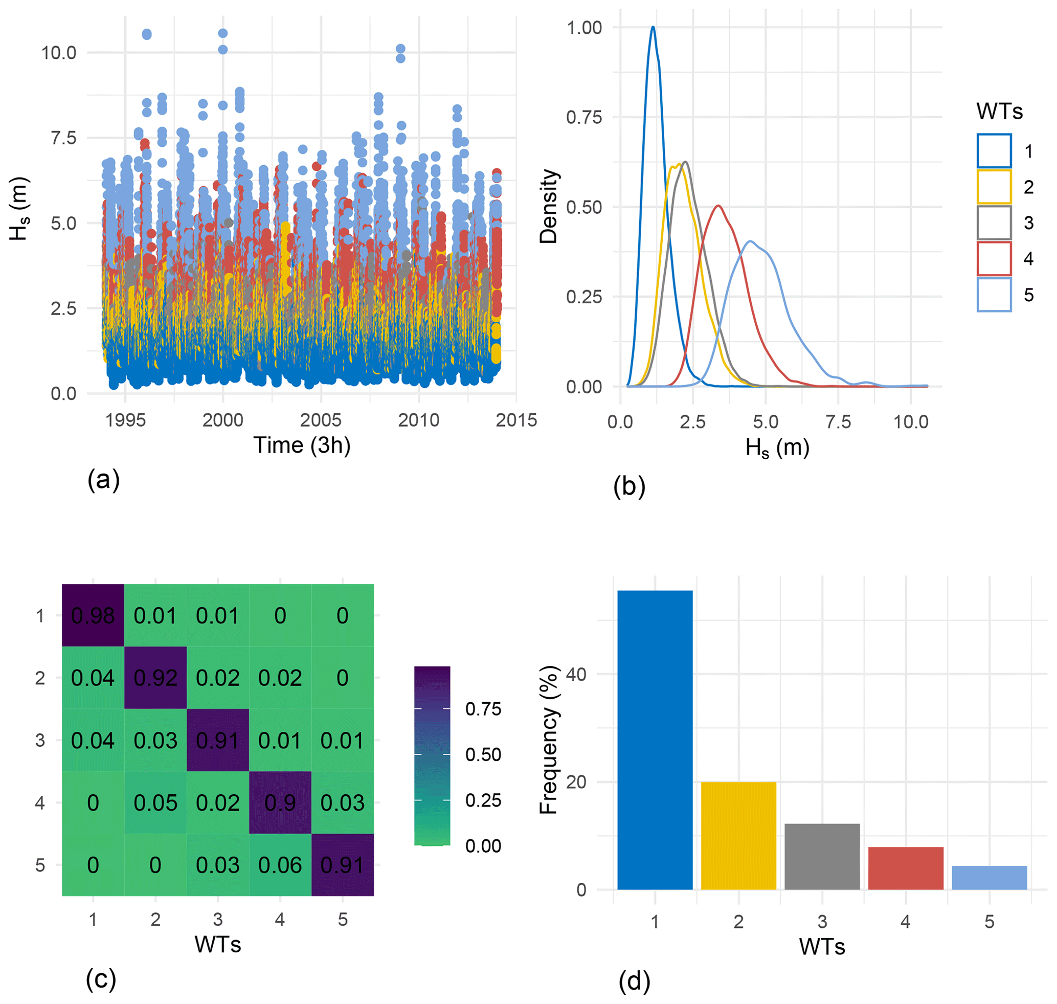
Figure 13(a) Time series of Hs as a function of WTs. (b) Empirical density of Hs as a function of WTs. (c) Transition matrix of WTs. (d) Frequency of occurrence of WTs. All figures correspond to the calibration period.
5.4 The case of two weather types
The statistical downscaling model described in the previous section has K+2 hyperparameters, which include the ridge regularization parameter λ (as defined in Eq. 12), the K associated ridge regularization parameters for each weather type (as defined in Eq. 14), and the number of weather types (K). Due to the large number of possible combinations, it is not computationally feasible to optimize all of these hyperparameters simultaneously using traditional cross-validation methods. As an alternative, we propose a simpler approach. We first select λ by considering only two weather types. Next, we determine the optimal number of weather types for this fixed value of λ. Finally, we choose a common value for ridge regularization for all weather types.
The most usual approach to choosing the regularization parameter λ of the ridge regression consists of performing cross-validation and taking the value of λ, which minimizes a prediction error, typically the RMSE. In the current work, we also intend to obtain a physically interpretable model in addition to forecast accuracy. Interpretability will be quantified as follows. First, the k-means clustering algorithm is used on the contributions to identify the leading two clusters. The resulting clusters are then compared with the sea-state classification obtained using the energy spectrum partitioning in HOMERE. The sea states chosen for the comparison are wind sea and swell, and the agreement between the two clusterings is measured using the classification accuracy
where “correct predictions” denotes the number of observations that are well classified by the model, meaning the number of observations that are classified as swell (wind sea) by the energy spectrum partitioning algorithm and as class “1” (“2”) by the regression-guided clustering algorithm.
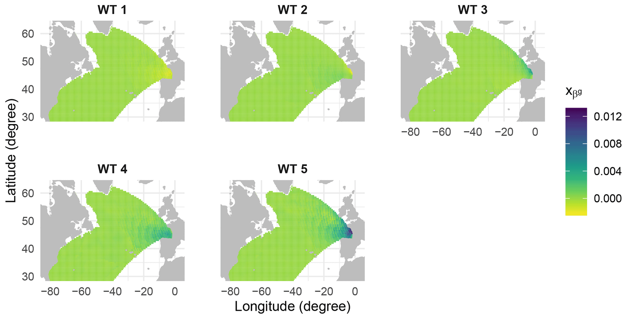
Figure 14Mean of minus the global mean for the five WTs.
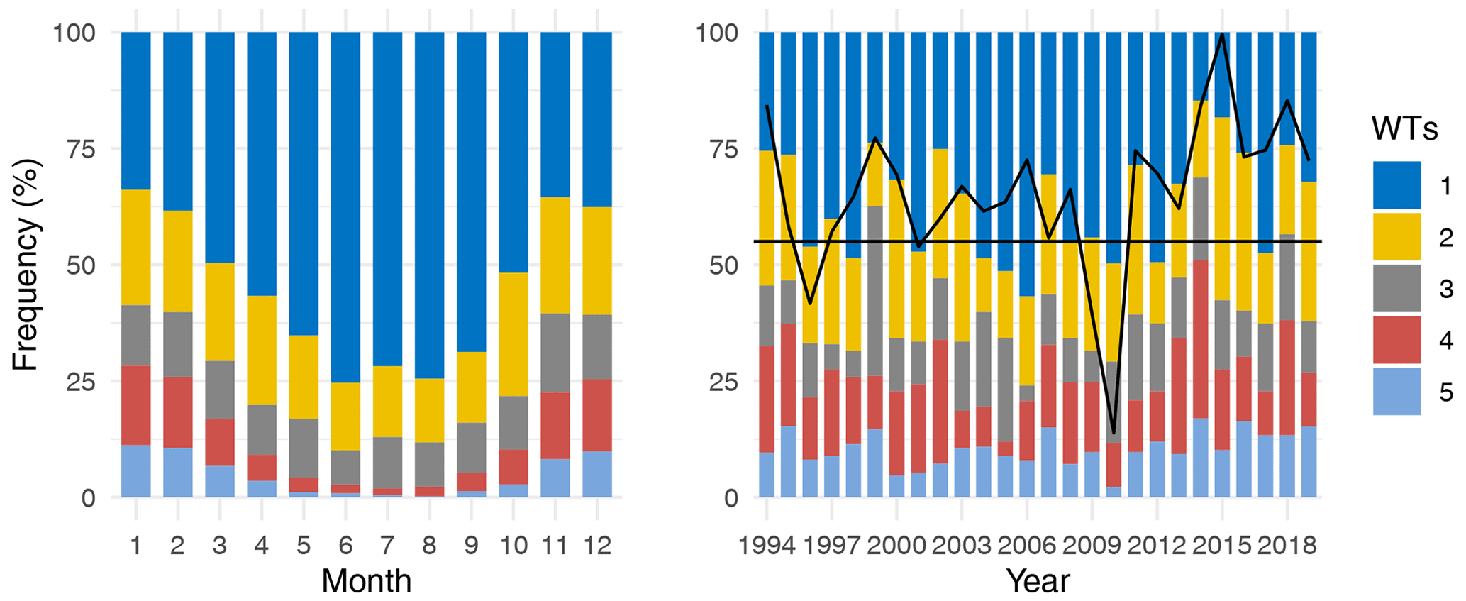
Figure 15Monthly and annual (in December–January–February) frequency occurrence of WTs in the calibration period. The continuous black line corresponds to the mean annual winter (DJF) time series of the NAO (North Atlantic Oscillation) index, and the horizontal black line indicates when NAO is less or greater than zero. When the continuous black line is below the horizontal line, the NAO is less than zero.
For the purpose of brevity, we only present the results of the weather types in Gironde, as they were found to be consistent in the other two locations. Figure 8 shows that the value of λ that gives the optimal classification accuracy is greater than that of the optimal RMSE. Figure 9 shows the estimated global coefficients β(g) using the two different optimal values of the regularization parameter λ. The coefficients obtained using λ that gives the maximum classification accuracy are smoother than the ones obtained when minimizing the RMSE and generally decrease as the distance between the source and target points increases. In this study, the optimal value of the regularization parameter, λ, is chosen based on its ability to produce interpretable coefficients and weather types. The primary focus is on the interpretability, and as such, the selected λ that yields the highest classification accuracy is prioritized, even if it results in a non-significant increase in RMSE compared to the value that yields the minimum RMSE. The optimization of RMSE will be considered in the next steps.
Table 1Contingency table of k-mean clusters (1 and 2) and HOMERE sea-state classes (swell and sea state) in the calibration period.
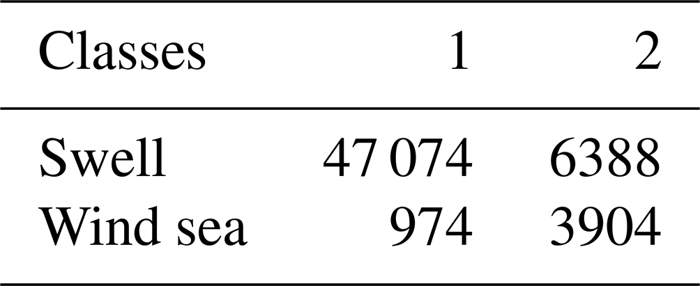
Figure 10 shows the times series of Hs and the corresponding empirical density with respect to the clusters in the calibration period. The most probable cluster is the first one (82 %), which corresponds mostly to swells, and the second cluster corresponds to wind seas (Table 1). To understand the difference between the two clusters, we define the anomaly of in each cluster 1 and 2 as and , respectively,
where and are the mean of at cluster 1 and 2, respectively; and is the global mean of . For the first cluster, the local wind around the target point contributes less than the global mean in Hs (Fig. 11). Grid points far from the target point contribute more, which is expected when swell systems dominate. In contrast, in the second cluster, generally associated with wind sea, local wind contributes more than the global mean in Hs. The fluctuations observed in Figs. 9 and 11 (also in Fig. 14 in the next section) may be attributed to two factors: the loss of smoothness in the data due to preprocessing steps such as travel time and temporal width, and the inherent nature of least squares estimates to alternate between positive and negative values when dealing with highly correlated covariates. The use of ridge regression, which smoothes the coefficients in comparison to ordinary least squares, still exhibits oscillations. As seen in Fig. 9, these oscillations are more significant when the ridge penalty is lower.
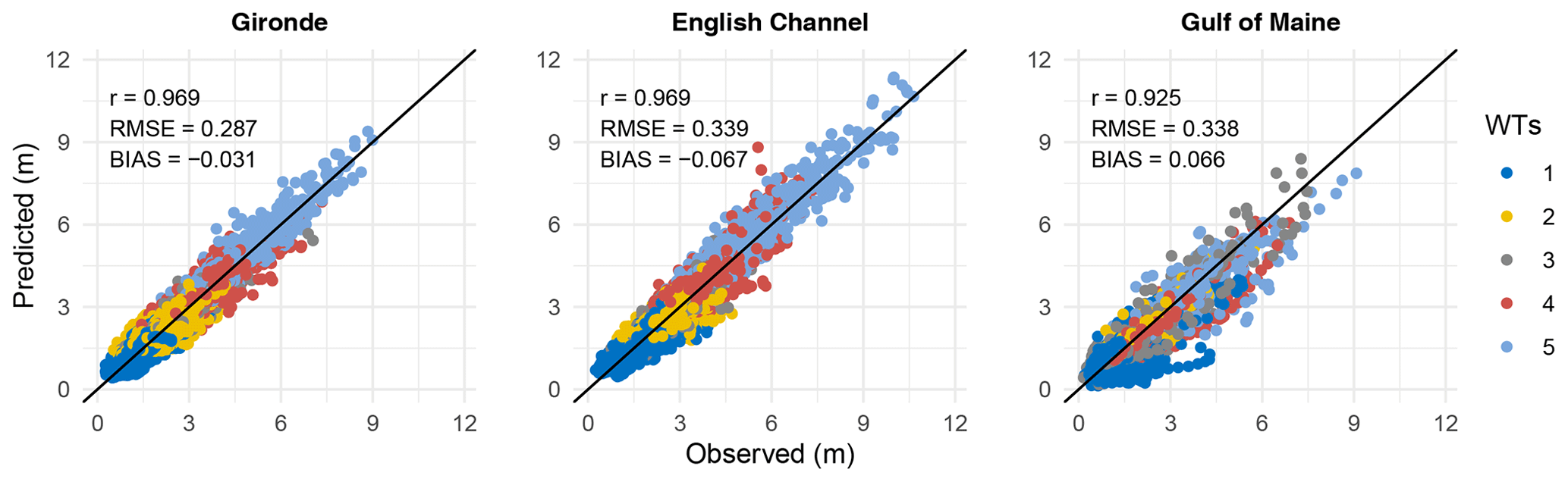
Figure 16Observed versus predicted values of Hs using the model (14) in the validation period at the three locations considered.
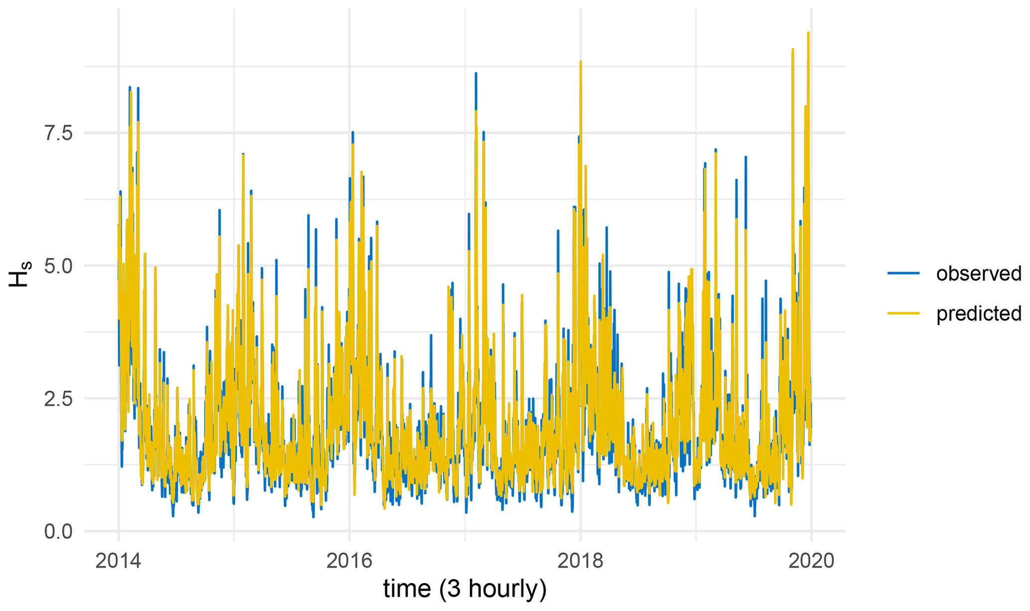
Figure 17Time series of observed and predicted values of Hs in the validation period in Gironde.
In this section, the methodology's results are presented. As for the last section, the results of the weather types were found to be consistent across the three studied locations; therefore, only the results for Gironde will be displayed. Subsequently, the overall methodology results for all three locations will be provided (see Fig. 16).
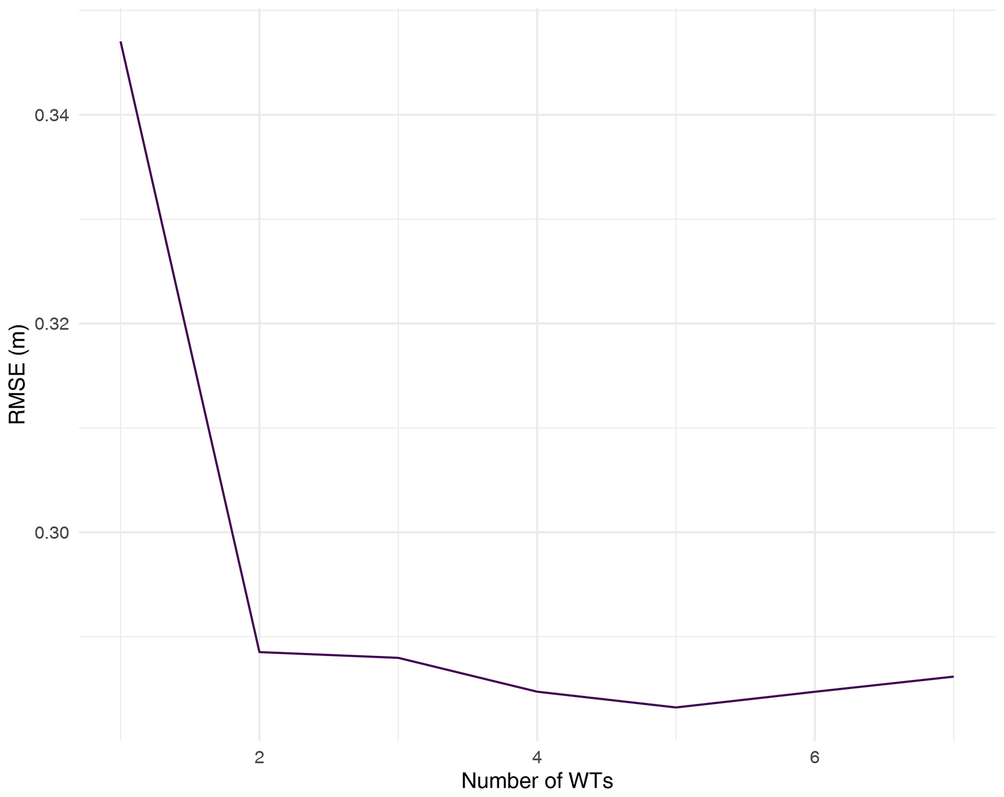
The clusters obtained in the last section seem to be interpretable and correspond to sea-state classes obtained from the energy partitioning algorithm provided by HOMERE (Boudière et al., 2013) (accuracy =0.87). However, the number of clusters K may be greater than 2; therefore, a validation analysis is done to select the optimal number of WTs. To do that, for each number of WTs (from 1 to 8), model (14) is fitted using the calibration period and evaluated using the validation period. Figure 12 illustrates the RMSE of Hs as a function of the number of WTs. The RMSE is stabilized for a number of WTs greater or equal to 5, and the RMSE decreases significantly from 1 to 5 WTs. We therefore chose the number of WTs to be 5.
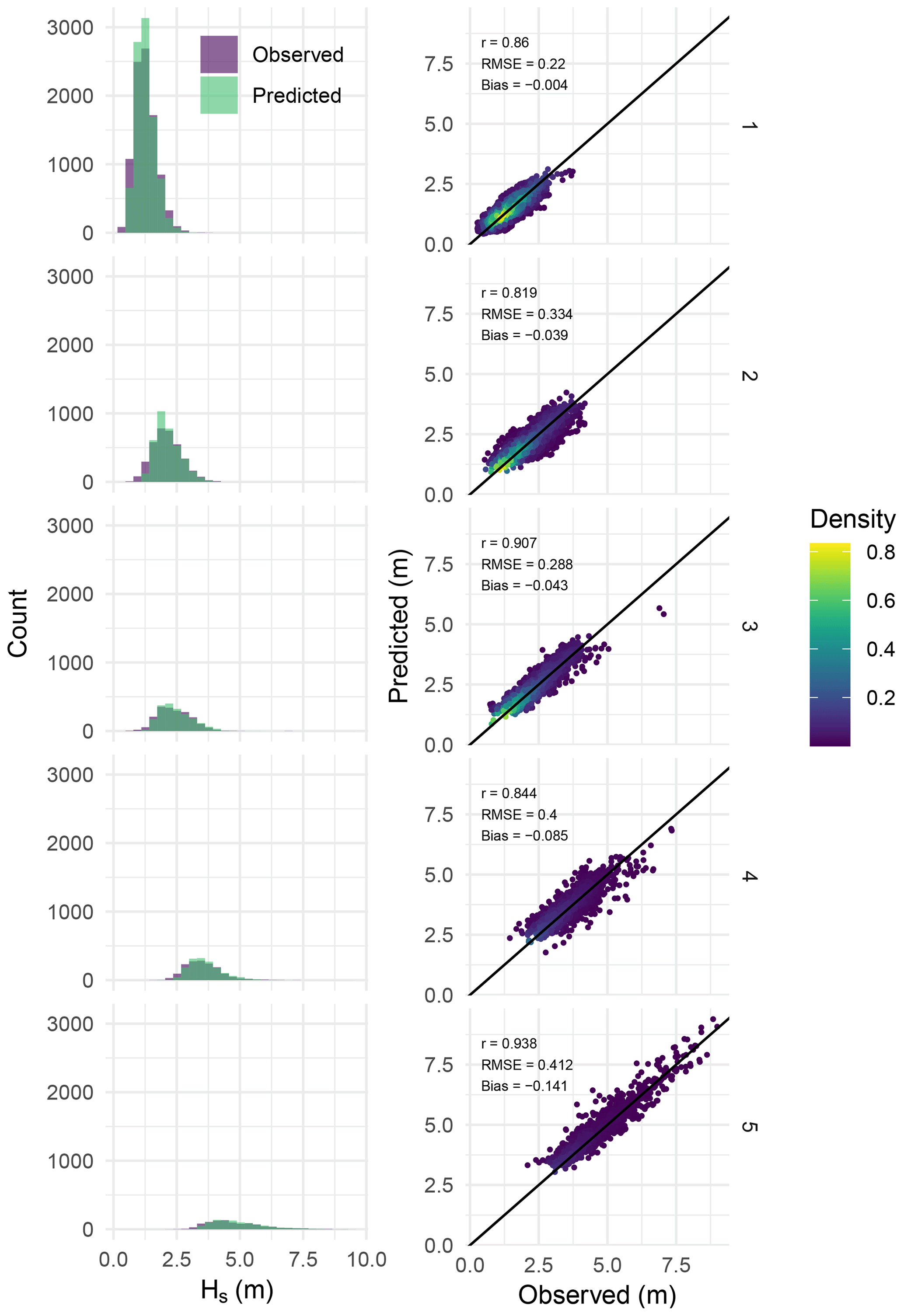
Figure 18Left panel: histogram of observed versus predicted Hs at each WT. Right panel: scatter plot of observed versus predicted Hs. Both in the validation period.
Figure 13 shows the time series of Hs and its empirical density as a function of the five WTs. Note that the weather types were manually arranged in ascending order according to the magnitude of Hs. The resulting WTs depend on the value of Hs; for example, the first WT corresponds to small values of Hs, and the fifth corresponds to extremes. In increasing order, the other clusters (2 to 4) correspond to intermediate values of Hs. The bottom right panel of Fig. 13 shows the frequency of occurrence of WTs. The first WT is the most likely, and the fifth one has the smallest probability of occurrence. The transition matrix in the bottom left panel shows that the self-transition probabilities are greater than 0.9 for all WTs, meaning that the WTs are consistent in time. Note that some transition probabilities are precisely zero; for example, the transition probabilities from the first to the fourth and the fifth WT are equal to zero. This means that the probability of being in extreme sea states after being in the first WT is zero.
Figure 14 shows the mean of at each WT where
where is the mean of at the ith WT, and is the global mean of . For the first and second WT, contributions of source points far from the target points are greater than the global mean. Therefore, these two classes may correspond to swells. In the third WT, the local wind contributes more, with moderate winds, in the variance of Hs. The fourth one can be considered as a composition of wind sea and swells given that local and far source points contribute to the variance of Hs. Finally, the fifth WT corresponds to the wind sea, where the local source points contribute with the highest intensities of winds creating the highest waves.
The monthly variability of WTs is shown in the left panel of Fig. 15. As expected, the fifth and fourth WTs occur primarily in winter (December–January–February), and the first WT, which corresponds mainly to swells, often occurs during summer. The long-term winter variability of frequency of occurrence of WTs is shown in the right panel of Fig. 15. The continuous black line corresponds to the mean annual winter of NAO index (Barnston and Livezey, 1987) from 1994 to 2019. The horizontal black line indicates when NAO is greater or less than zero. Figure 15 suggests that there is a correlation between the long-term variability of weather types and the North Atlantic Oscillation (NAO) index. For instance, the winter of 2010 exhibited a lower frequency of extreme waves and corresponded with a low NAO index, while the most extreme sea states were observed in 2014, which coincided with a high NAO index. This correlation is consistent with previous research, such as in Charles et al. (2012), which reported that winter waves tend to have larger significant wave heights (Hs) during the positive phase of the NAO and smaller Hs during the negative phase of the NAO.
The results of the model described in Eq. (14) during the validation period for the three studied locations are presented in Figs. 16 and 17 for Gironde. The model performs well in predicting Hs at Gironde and the English Channel. However, it exhibits less accuracy in the Gulf of Maine, which can be attributed to the complex wave climate in this area due to factors such as bathymetry, islands, breaking waves, and frequent storm activity (Panchang et al., 2008). Comparing these results with those of the local model in Fig. 2, it appears that considering the global predictor is essential to explain the variability of Hs. Figure 18 illustrates the performance of the downscaling model at each weather type in the validation period. It can be seen that the model in WT 1, 2, and 4 explains less of the variability of Hs compared with the model in WT 3 and 5. This might be explained by the fact that in these WTs (1, 2, and 4), the model has to consider source points that cover the swell generation, as seen in Fig. 14, which means that numerous source points contributes to the variability of Hs. In contrast, in WT 3 and 5, waves are mainly generated by local wind (Fig. 14); therefore, the model considers mainly local source points.
This study proposes a method that describes the spatiotemporal relationship between wind and the significant wave height (Hs). At first, the local model, based on a linear regression between the local wind and Hs, is constructed. However, the model poorly explains the variability of Hs given that the model does not consider the swell generation. Therefore, the global predictor was defined to account for both wind sea and swells. The global predictor is based on the target-projected wind, which is the wind that goes from source points to the target point in a great circle path. After wind projection, the spatial coverage of the predictor is defined based on the assumption that waves travel along a great circle path. Then its temporal coverage is defined based on two parameters, the travel time of waves and the temporal width. Both parameters exhibit spatial structure and increase as the distance between the source and target points increases.
The statistical downscaling model combines the local and global predictors to predict Hs using a weather-types-based model. The weather types were constructed using a regression-guided clustering algorithm. The comparison between the HOMERE sea-state classes (wind sea and swell) and two clusters obtained by the clustering algorithm shows a significant resemblance. The predictive model consists of fitting linear regression with ridge penalty between the predictors and the predictand in each WT, and the validation analysis shows that the optimal number of WTs is five. The obtained weather types are interpretable and correspond to different wave systems. The results of the downscaling model show its skill in predicting Hs, even for large values, which are often important for operational purposes. The proposed method can be used for various operational applications depending on the availability and quality of wind data. These applications include hindcasting, short-term forecasting, and climate projections. In the case of climate projections, the method can use bias-corrected output from global climate models (GCMs). The statistical method presented in this study is validated at three locations, and its ability to accurately predict Hs is demonstrated; the method may be therefore generalizable and can be extended to other locations. For locations nearshore, it may be necessary to take into account other local characteristics such as bathymetry and currents, as these factors can significantly impact wave behavior. In addition, the assumption of great circle wave propagation may not be valid for these locations, and alternative wave propagation models may be considered. Another limitation of the proposed methodology is its limited scope in predicting only significant wave height (Hs). To fully characterize a sea state, other parameters such as wave period and direction should also be taken into account. Future research should investigate the generalizability of the methodology to other sea-state parameters.
In this paper, we introduced a methodology based on observed weather types, constructed prior to the regression problem using a clustering algorithm. For future research, these weather types could be treated as latent variables within a mixture regression framework, which can be estimated using the expectation maximization (EM) algorithm. This approach would evaluate variables according to Hs predictions, which can yield to statistically optimal estimates.
The hindcast HOMERE data are available on their website: https://doi.org/10.12770/cf47e08d-1455-4254-955e-d66225c9dc90 (Accensi and Maisondieu, 2015). The wind data are available from the CFSR website: https://climatedataguide.ucar.edu/climate-data/climate-forecast-system-reanalysis-cfsr (Saha et al., 2010). Finally, the NAO index is obtained from the National Oceanic and Atmospheric Administration website: https://www.cpc.ncep.noaa.gov/products/precip/CWlink/pna/nao.shtml (Compo et al., 2011). The processed data used in this work can be found in https://doi.org/10.5281/zenodo.5845423 (Obakrim et al., 2022b), and the R notebooks are available in https://doi.org/10.5281/zenodo.5845250 (Obakrim et al., 2022a).
Conceptualization: SO, VM, NR, and PA; methodology: SO, VM, NR, and PA; data curation: SO and NR; data visualization: SO; software: SO; supervision: VM, NR, and PA; and writing original draft: SO. All authors approved the final submitted paper.
The contact author has declared that none of the authors has any competing interests.
Publisher’s note: Copernicus Publications remains neutral with regard to jurisdictional claims in published maps and institutional affiliations.
The authors express their gratitude to the editor and anonymous reviewers for their valuable input and extensive feedback, which greatly enhanced the quality of the work.
This paper was edited by Xiaolan Wang and reviewed by three anonymous referees.
Accensi, M. and Maisondieu, C.: HOMERE. Ifremer Laboratoire Comportement des Structures en Mer, Ifremer Laboratoire Spatial et In terfaces Air Mer, [data set], https://doi.org/10.12770/cf47e08d-1455-4254-955e-d66225c9dc90, 2015. a
Anderson, D., Rueda, A., Cagigal, L., Antolinez, J., Mendez, F., and Ruggiero, P.: Time-varying emulator for short and long-term analysis of coastal flood hazard potential, J. Geophys. Res.-Oceans, 124, 9209–9234, 2019. a
Ardhuin, F. and Orfila, A.: Wind waves, New Frontiers in Operational Oceanography, 14, 393–422, 2018. a, b, c, d, e
Ardhuin, F., Hanafin, J., Quilfen, Y., Chapron, B., Queffeulou, P., Obrebski, M., Sienkiewicz, J., and Vandemark, D.: Calibration of the IOWAGA global wave hindcast (1991–2011) using ECMWF and CFSR winds, in: Proceedings of the 2011 International Workshop on Wave Hindcasting and Forecasting and 3rd Coastal Hazard Symposium, Kona, HI, USA, November 2014, vol. 30, 2011. a
Ardhuin, F., Stopa, J. E., Chapron, B., Collard, F., Husson, R., Jensen, R. E., Johannessen, J., Mouche, A., Passaro, M., Quartly, G. D., Swail, V., and Young, I.: Observing sea states, Front. Mar. Sci., 124, https://doi.org/10.3389/fmars.2019.00124, 2019. a
Barnston, A. G. and Livezey, R. E.: Classification, seasonality and persistence of low-frequency atmospheric circulation patterns, Mon. Weather Rev., 115, 1083–1126, 1987. a
Boudière, E., Maisondieu, C., Ardhuin, F., Accensi, M., Pineau-Guillou, L., and Lepesqueur, J.: A suitable metocean hindcast database for the design of Marine energy converters, International Journal of Marine Energy, 3, e40–e52, 2013. a, b
Cagigal, L., Rueda, A., Anderson, D., Ruggiero, P., Merrifield, M. A., Montaño, J., Coco, G., and Méndez, F. J.: A multivariate, stochastic, climate-based wave emulator for shoreline change modelling, Ocean Model., 154, 101695, https://doi.org/10.1016/j.ocemod.2020.101695, 2020. a
Camus, P., Méndez, F. J., Losada, I. J., Menéndez, M., Espejo, A., Pérez, J., Rueda, A., and Guanche, Y.: A method for finding the optimal predictor indices for local wave climate conditions, Ocean Dynam., 64, 1025–1038, 2014a. a, b, c, d
Camus, P., Menendez, M., Mendez, F. J., Izaguirre, C., Espejo, A., Canovas, V., Perez, J., Rueda, A., Losada, I. J., and Medina, R.: A weather-type statistical downscaling framework for ocean wave climate, J. Geophys. Res.-Oceans, 119, 7389–7405, 2014b. a
Camus, P., Rueda, A., Méndez, F. J., and Losada, I. J.: An atmospheric-to-marine synoptic classification for statistical downscaling marine climate, Ocean Dynam., 66, 1589–1601, 2016. a
Casas-Prat, M., Wang, X. L., and Sierra, J. P.: A physical-based statistical method for modeling ocean wave heights, Ocean Model., 73, 59–75, 2014. a
Charles, E., Idier, D., Thiébot, J., Le Cozannet, G., Pedreros, R., Ardhuin, F., and Planton, S.: Present wave climate in the Bay of Biscay: spatiotemporal variability and trends from 1958 to 2001, J. Climate, 25, 2020–2039, 2012. a
Compo, G. P., Whitaker, J. S., Sardeshmukh, P. D., Matsui, N., Allan, R. J., Yin, X., Gleason, B. E., Vose, R. S., Rutledge, G., Bessemoulin, P., Brönnimann, S., Brunet, M., Crouthamel, R. I., Grant, A. N., Groisman, P. Y., Jones, P. D., Kruk, M., Kruger, A. C., Marshall, G. J., Maugeri, M., Mok, H. Y., Nordli, Ø., Ross, T. F., Trigo, R. M., Wang, X. L., Woodruff, S. D., and Worley, S. J.: The Twentieth Century Reanalysis Project, Q. J. Roy. Meteor. Soc., 137, 1–28, https://doi.org/10.1002/qj.776, 2011 (data available at : https://www.cpc.ncep.noaa.gov/products/precip/CWlink/pna/nao.shtml, last access: 31 May 2023). a
Costa, W., Idier, D., Rohmer, J., Menendez, M., and Camus, P.: Statistical Prediction of Extreme Storm Surges Based on a Fully Supervised Weather-Type Downscaling Model, Journal of Marine Science and Engineering, 8, 1028, https://doi.org/10.3390/jmse8121028, 2020. a
Hasselmann, K. F., Barnett, T. P., Bouws, E., Carlson, H., Cartwright, D. E., Eake, K., Euring, J., Gicnapp, A., Hasselmann, D., Kruseman, P., and Meerburg, A.: Measurements of wind-wave growth and swell decay during the Joint North Sea Wave Project (JONSWAP), Ergaenzungsheft zur Deutschen Hydrographischen Zeitschrift, Reihe A, https://hdl.handle.net/21.11116/0000-0007-DD3C-E, 1973. a
Hegermiller, C., Antolinez, J. A., Rueda, A., Camus, P., Perez, J., Erikson, L. H., Barnard, P. L., and Mendez, F. J.: A multimodal wave spectrum–based approach for statistical downscaling of local wave climate, J. Phys. Oceanogr., 47, 375–386, 2017. a
Hemer, M. A., Wang, X. L., Weisse, R., and Swail, V. R.: Advancing wind-waves climate science: The COWCLIP project, B. Am. Meteorol. Soc., 93, 791–796, 2012. a
Hessami, M., Gachon, P., Ouarda, T. B., and St-Hilaire, A.: Automated regression-based statistical downscaling tool, Environ. Modell. Softw., 23, 813–834, 2008. a
Hoerl, A. E. and Kennard, R. W.: Ridge regression: Biased estimation for nonorthogonal problems, Technometrics, 12, 55–67, 1970. a, b
Laugel, A., Menendez, M., Benoit, M., Mattarolo, G., and Méndez, F.: Wave climate projections along the French coastline: dynamical versus statistical downscaling methods, Ocean Model., 84, 35–50, 2014. a, b, c
Mahajan, V., Jain, A. K., and Bergier, M.: Parameter estimation in marketing models in the presence of multicollinearity: An application of ridge regression, J. Marketing Res., 14, 586–591, 1977. a
Mori, N., Shimura, T., Yasuda, T., and Mase, H.: Multi-model climate projections of ocean surface variables under different climate scenarios–Future change of waves, sea level and wind, Ocean Eng., 71, 122–129, 2013. a
Obakrim, S., Ailliot, P., Monbet, V., and Raillard, N.: Statistical downscaling of significant wave height: code for data preparation and model, Zenodo [data set], https://doi.org/10.5281/zenodo.5845250, 2022a. a
Obakrim, S., Ailliot, P., Monbet, V., and Raillard, N.: Statistical downscaling of significant wave height: data, Zenodo [data set], https://doi.org/10.5281/zenodo.5845423, 2022b. a
Panchang, V. G., Jeong, C., and Li, D.: Wave climatology in coastal Maine for aquaculture and other applications, Estuar. Coast., 31, 289–299, 2008. a, b
Pérez, J., Méndez, F. J., Menéndez, M., and Losada, I. J.: ESTELA: a method for evaluating the source and travel time of the wave energy reaching a local area, Ocean Dynam., 64, 1181–1191, 2014. a, b, c
Saha, S., Moorthi, S., Pan, H.-L., Wu, X., Wang, J., Nadiga, S., Tripp, P., Kistler, R., Woollen, J., Behringer, D., and Liu, H.: The NCEP climate forecast system reanalysis, B. Am. Meteorol. Soc., 91, 1015–1058, 2010 (data available at: https://climatedataguide.ucar.edu/climate-data/climate-forecast-system-reanalysis-cfsr, last access: 31 May 2023). a, b
Tolman, H. L.: User manual and system documentation of WAVEWATCH III TM version 3.14, Technical note, MMAB Contribution, 276, 220 pp., 2009. a
Tracy, B., Devaliere, E., Hanson, J., Nicolini, T., and Tolman, H.: Wind sea and swell delineation for numerical wave modeling, in: 10th international workshop on wave hindcasting and forecasting & coastal hazards symposium, JCOMM Tech. Rep, 11 November 2007, North Shore, Oahu, Hawaii, vol. 41, p. 1442, 2007. a
van Wieringen, W. N.: Lecture notes on ridge regression, arXiv [preprint], https://doi.org/10.48550/arXiv.1509.09169, 2015. a
Wang, X. L., Swail, V. R., and Cox, A.: Dynamical versus statistical downscaling methods for ocean wave heights, Int. J. Climatol., 30, 317–332, 2010. a
Young, I. R.: Wind generated ocean waves, Elsevier, 1999. a