Parametric model for post-processing visibility ensemble forecasts

Although, by now, ensemble-based probabilistic forecasting is the most advanced approach to weather prediction, ensemble forecasts still suffer from a lack of calibration and/or display systematic bias, thus requiring some post-processing to improve their forecast skill. Here, we focus on visibility, a weather quantity that plays a crucial role in, for example, aviation and road safety or ship navigation, and we propose a parametric model where the predictive distribution is a mixture of a gamma and a truncated normal distribution, both right censored at the maximal reported visibility value. The new model is evaluated in two case studies based on visibility ensemble forecasts of the European Centre for Medium-Range Weather Forecasts covering two distinct domains in central and western Europe and two different time periods. The results of the case studies indicate that post-processed forecasts are substantially superior to raw ensembles; moreover, the proposed mixture model consistently outperforms the Bayesian model averaging approach used as a reference post-processing technique.

1 Introduction

Despite the continuous improvement of autoland, autopilot, navigation, and radar systems, visibility conditions are still critical in aviation and road safety and in ship navigation as well. Nowadays, visibility observations are obtained automatically; visibility sensors take the measurements of “the length of atmosphere over which a beam of light travels before its luminous flux is reduced to 5 % of its original value”¹, the quantity of which is called the meteorological optical range.

Visibility forecasts are generated with the help of numerical weather prediction (NWP) models either as direct model outputs or by utilizing various algorithms (see, e.g. Stoelinga and Warner, 1999; Gultepe et al., 2006; Wagh et al., 2023) to calculate visibility from forecasts of related weather quantities such as precipitation or relative humidity (Chmielecki and Raftery, 2011). Nowadays, the state-of-the-art approach to weather prediction is to issue ensemble forecasts by running an NWP model several times with perturbed initial conditions or different model parameterizations (Bauer et al., 2015; Buizza, 2018a). Hence, for a given location, time point, and forecast horizon, instead of having a point forecast, a forecast ensemble is issued. It opens the door for estimating the forecast uncertainty or even the probability distribution of the future weather variable (Gneiting and Raftery, 2005) and provides an important tool for forecast-based decision-making (Fundel et al., 2019). In particular, several recent studies (see Pahlavan et al., 2021; Parde et al., 2022) verify the superiority of probabilistic predictions in, for example, fog forecasting, which is one of the most frequent reasons for low visibility.

By now, all major weather centres operate ensemble prediction systems (EPSs); however, only a few have visibility among the forecasted parameters. For instance, since 2015, visibility has been part of the Integrated Forecast System (IFS; ECMWF, 2021) of the European Centre for Medium-Range Weather Forecasts (ECMWF; ECMWF Directorate, 2012); nevertheless, it is an experimental product, and “expectations regarding the quality of this product should remain low” (Owens and Hewson, 2018, Sect. 9.4). A further example is the Short-Range Ensemble Forecast System of the National Centers for Environmental Prediction, which covers the continental US, Alaska, and Hawaii regions (Zhou et al., 2009).

A typical problem with the ensemble forecasts is their under-dispersive and biased feature, which has been observed with several operational EPSs (see, e.g. Buizza et al., 2005) and can be corrected with some form of post-processing (Buizza, 2018b). In the last decades, a multitude of statistical calibration techniques have been proposed for a broad range of weather parameters; see Wilks (2018) or Vannitsem et al. (2021) for an overview of the most advanced approaches. Non-parametric methods usually represent predictive distributions via their quantiles estimated by some form of quantile regression (see, e.g. Friederichs and Hense, 2007; Bremnes, 2019), whereas parametric models such as Bayesian model averaging (BMA; Raftery et al., 2005) or ensemble model output statistics (EMOS; Gneiting et al., 2005) provide full predictive distributions of the weather variables at hand. The BMA predictive probability density function (PDF) of a future weather quantity is the weighted sum of individual PDFs corresponding to the ensemble members, where the form of the predictive PDF might be beneficial in situations when multimodal predictive distributions are required (see, e.g. Baran et al., 2019). In contrast, the EMOS (also referred to as non-homogeneous regression) predictive distribution is given by a single parametric family, where distributional parameters are given functions of the ensemble members. Furthermore, recently, machine-learning-based approaches have gained more and more popularity in ensemble post-processing, both in parametric frameworks (see, e.g. Rasp and Lerch, 2018; Ghazvinian et al., 2021; Baran and Baran, 2024) and in non-parametric contexts (Bremnes, 2020); for a systematic overview of the state-of-the-art techniques, see Schultz and Lerch (2022). Finally, in the case of discrete quantities, such as total cloud cover (TCC), the predictive distribution is a probability mass function, and post-processing can be considered to be a classification problem, where both parametric techniques (Hemri et al., 2016) and advanced machine-learning-based classifiers can be applied (Baran et al., 2021).

Although, as mentioned, visibility forecasts are far less reliable than ensemble forecasts of other weather parameters (see, e.g. Zhou et al., 2012), only a few of the above-mentioned methods are adapted to this particular variable. Chmielecki and Raftery (2011) consider a BMA approach where each individual predictive PDF consists of a point mass at the maximal reported visibility and a beta distribution, which models the remaining visibility values. Ryerson and Hacker (2018) propose a non-parametric method for calibrating short-range visibility predictions obtained using the Weather Research and Forecasting Model (Ryerson and Hacker, 2014). Furthermore, since most synoptic-observation (SYNOP) stations report visibility in discrete values according to the WMO suggestions, in a recent study, Baran and Lakatos (2023) investigated the approach of Hemri et al. (2016) and Baran et al. (2021) and obtained (discrete) predictive distributions of visibility with the help of proportional odds logistic regression and multilayer perceptron neural network classifiers.

In the present article, we develop a novel parametric post-processing model for visibility ensemble forecasts where the predictive distribution is a mixture of a gamma and a truncated normal distribution, both right censored at the maximal reported visibility value. The proposed mixture model is applied in two case studies that focus on ECMWF visibility ensemble forecasts covering two distinct domains in central and western Europe and two different time periods. As a reference post-processing approach, we consider the BMA model of Chmielecki and Raftery (2011); nonetheless, we report the predictive performance of climatological and raw ensemble forecasts as well.

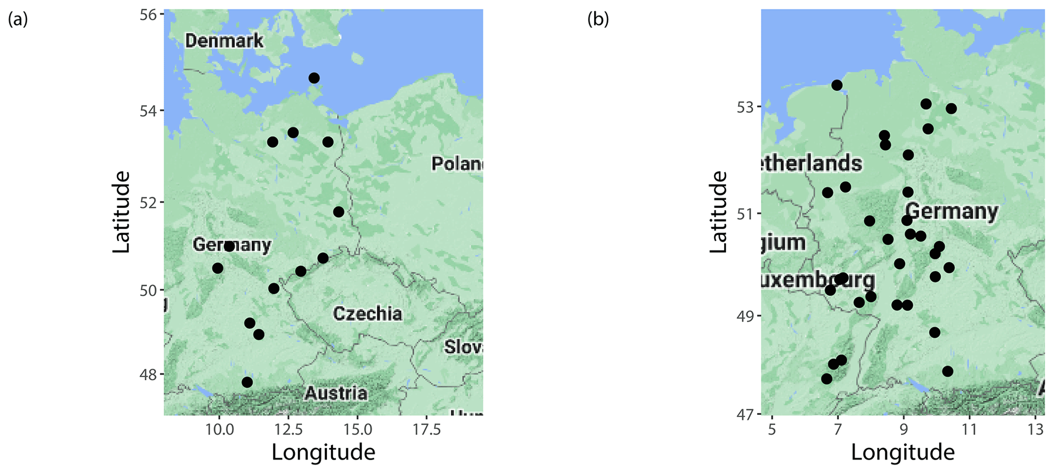
Figure 1 Locations of SYNOP observation stations corresponding to (a) ECMWF forecasts for 2020–2021 and (b) EUPPBench benchmark dataset.

The paper is organized as follows. Section 2 briefly introduces the visibility datasets considered in the case studies. The proposed mixture model, the reference BMA approach, training data selection procedures, and tools of forecast verification are provided in Sect. 3, followed by the results for the two case studies presented in Sect. 4. Finally, concluding remarks and the lessons learned can be found in Sect. 5.

2 Data

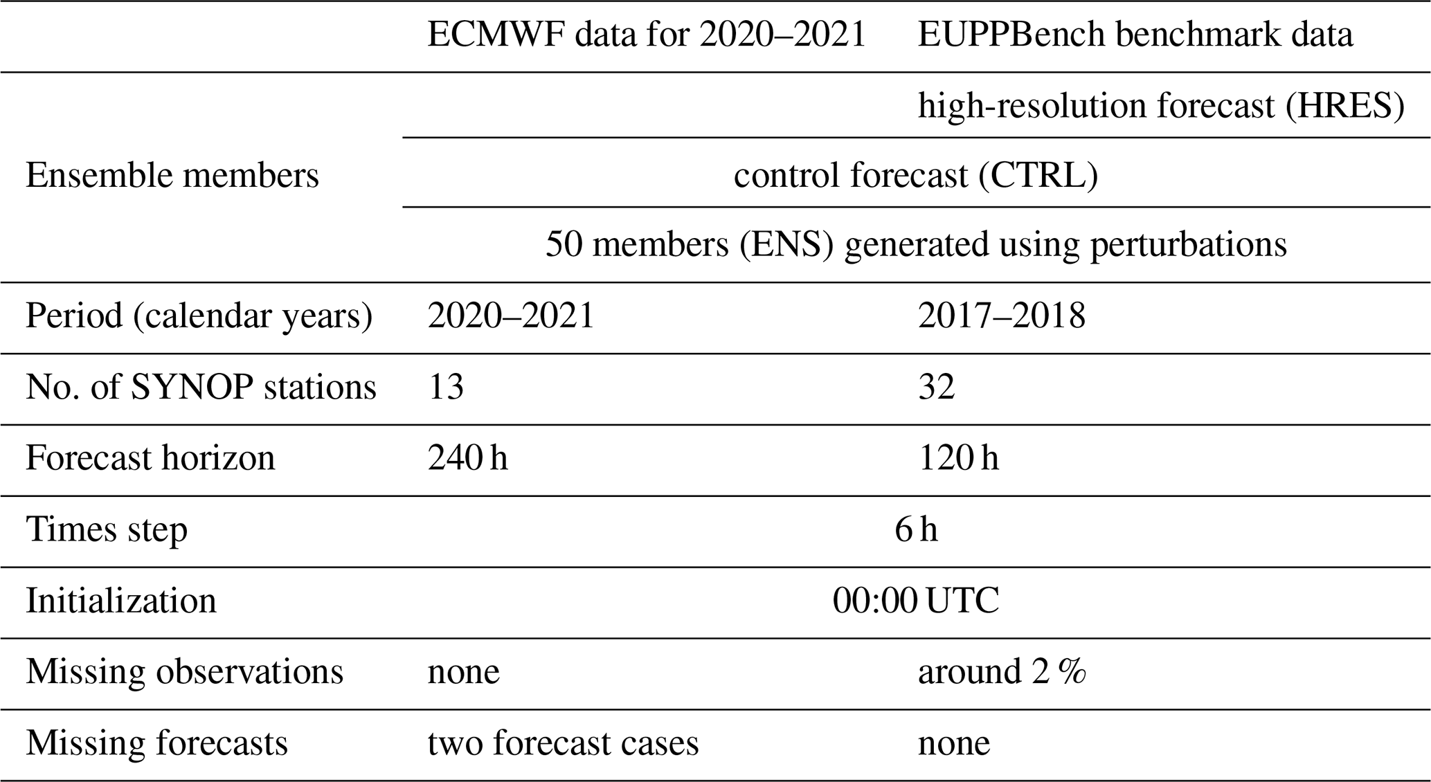
In the case studies of Sect. 4, we evaluate the mixture model proposed in Sect. 3.1 using ECMWF visibility ensemble forecasts (given in 1 m steps) and corresponding validating observations (reported in 10 m increments) covering two different time periods and having disjointed but geographically close ensemble domains. In fact, we consider subsets of the datasets studied in Baran and Lakatos (2023) by selecting only those locations where the resolution of the reported observations is close to that of the forecasts and can be treated as continuous. The first dataset comprises the operational 51-member ECMWF visibility ensemble forecasts for the calendar years 2020 and 2021, whereas the second contains visibility data of the EUPPBench benchmark dataset (Demaeyer et al., 2023) for calendar years 2017–2018. The locations of the investigated SYNOP stations are given in Fig. 1, while Table 1 provides an overview of both studied datasets.

Table 1 Overview of the studied datasets.

3 Parametric post-processing of visibility

As mentioned in the Introduction, EMOS is a simple and efficient tool for post-processing ensemble weather forecasts (see also Vannitsem et al., 2021). However, as it fits a single probability law to the forecast ensemble chosen from a given parametric distribution family, EMOS is usually not flexible enough to model multimodal predictive distributions. A natural approach is to consider a mixture of several probability laws, which is also the fundamental idea of the BMA models. Furthermore, visibility is non-negative, and the reported observations are often limited to a certain value (in our case studies to 75 and 70 km); this restriction should be taken into account too. A possible solution is to censor a non-negative predictive distribution from above or to mix a continuous law and a point mass at the maximal reported visibility value. The former approach appears in the mixture model proposed in Sect. 3.1, whereas the reference BMA model of Chmielecki and Raftery (2011) described briefly in Sect. 3.2 is an example of the latter.

In the following sections, let $f_{\mathrm{1}},f_{\mathrm{2}},\mathrm{\dots },f_{\mathrm{52}}$ denote a 52-member ECMWF visibility ensemble forecast for a given location, time point, and forecast horizon, where f₁=f_HRES and f₂=f_CTRL are the high-resolution and control members, respectively, whereas $f_{\mathrm{3}},f_{\mathrm{4}},\mathrm{\dots },f_{\mathrm{52}}$ correspond to the 50 members generated using perturbed initial conditions. These members, which we will denote with $f_{\mathrm{ENS},\mathrm{1}},f_{\mathrm{ENS},\mathrm{2}},\mathrm{\dots },f_{\mathrm{ENS},\mathrm{50}}$, lack individually distinguishable physical features; hence, they are statistically indistinguishable and can be treated as exchangeable. In what follows, ${\stackrel{\mathrm{‾}}{f}}_{\mathrm{ENS}}$ and S_ENS will denote the mean and standard deviation of the 50 exchangeable ensemble members, respectively, and following the suggestions of, e.g. Fraley et al. (2010) or Wilks (2018), in the models presented in Sect. 3.1 and 3.2, these members will share the same parameters.

3.1 Mixture model

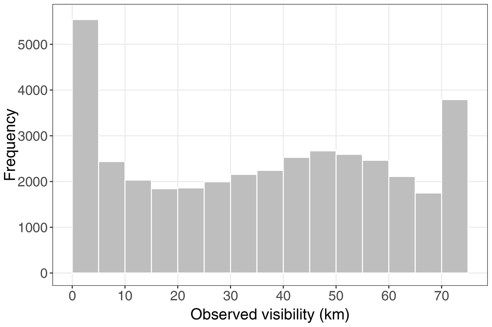
According to the climatological histogram of Fig. 2, a unimodal distribution is clearly not appropriate in relation to model visibility. One has to handle low-visibility values separately; there is a second hump at medium to large visibility, and censoring is required at the maximal reported value x_max.

Figure 2 Climatological frequency histogram of visibility for calendar years 2020–2021.

Let $g\left(x\right|\mathit{\kappa },\mathit{\theta })$ and $G\left(x\right|\mathit{\kappa },\mathit{\theta })$ denote the probability density function (PDF) and cumulative distribution function (CDF) of a gamma distribution Γ(κ,θ), with shape κ>0 and scale θ>0, respectively, while the notations $h\left(x\right|\mathit{\mu },{\mathit{\sigma }}^{\mathrm{2}})$ and $H\left(x\right|\mathit{\mu },{\mathit{\sigma }}^{\mathrm{2}})$ are used for the PDF and the CDF of a normal distribution 𝒩₀(μ,σ²), with location μ and scale σ>0 left truncated at zero. Furthermore, denote the PDFs of the censored versions of these laws using $g^{\mathrm{c}}\left(x\right|\mathit{\kappa },\mathit{\theta })$ and $h^{\mathrm{c}}\left(x\right|\mathit{\mu },{\mathit{\sigma }}^{\mathrm{2}})$, that is

$$\begin{array}{ll}{\displaystyle }{g}^{\mathrm{c}}\left(x\right|\mathit{\kappa },\mathit{\theta }):=& {\displaystyle }g\left(x\right|\mathit{\kappa },\mathit{\theta }){\mathbb{I}}_{\mathit{\{}x<x_{\max }\mathit{\}}}\\ {\displaystyle }& {\displaystyle }+(\mathrm{1}-G(x_{\max }|\mathit{\kappa },\mathit{\theta })){\mathbb{I}}_{\mathit{\{}x=x_{\max }\mathit{\}}},\\ {\displaystyle }{h}^{\mathrm{c}}\left(x\right|\mathit{\mu },{\mathit{\sigma }}^{\mathrm{2}}):=& {\displaystyle }h\left(x\right|\mathit{\mu },{\mathit{\sigma }}^{\mathrm{2}}){\mathbb{I}}_{\mathit{\{}x<x_{\max }\mathit{\}}}\\ {\displaystyle }& {\displaystyle }+(\mathrm{1}-H(x_{\max }|\mathit{\mu },{\mathit{\sigma }}^{\mathrm{2}})){\mathbb{I}}_{\mathit{\{}x=x_{\max }\mathit{\}}},\end{array}$$

where 𝕀_A denotes the indicator function of a set A.

The proposed predictive distribution of visibility is a mixture of censored gamma and censored truncated normal distributions:

$$\begin{array}{}\text{(1)}& p\left(x\right|\mathit{\kappa },\mathit{\theta },\mathit{\mu },{\mathit{\sigma }}^{\mathrm{2}},\mathit{\omega })=(\mathrm{1}-\mathit{\omega }\left)g^{\mathrm{c}}\right(x|\mathit{\kappa },\mathit{\theta })+\mathit{\omega }{h}^{\mathrm{c}}\left(x\right|\mathit{\mu },{\mathit{\sigma }}^{\mathrm{2}}),\end{array}$$

where both the weight $\mathit{\omega }\in [\mathrm{0},\mathrm{1}]$ and the parameters of the component distributions depend on the ensemble forecast. In particular,

$$\mathit{\omega }=\mathrm{1}/(\mathrm{1}+\exp (-\mathit{\gamma }{\stackrel{\mathrm{‾}}{f}}_{\mathrm{ENS}}\left)\right),$$

which is a smooth monotone function of ${\stackrel{\mathrm{‾}}{f}}_{\mathrm{ENS}}$. We remark, that this specific form of the weight is a result of a detailed data analysis, where various parametric functions of the ensemble forecast with range  [0,1]  had been tested, including the forecast-independent weight (see, e.g. Baran and Lerch, 2016). Furthermore, the mean m=κθ and variance v=κθ² of the uncensored gamma distribution Γ(κ,θ) are given as

$$\begin{array}{ll}{\displaystyle }m=a_{\mathrm{0}}& {\displaystyle }+a_{\mathrm{1}}^{\mathrm{2}}{f}_{\mathrm{HRES}}+a_{\mathrm{2}}^{\mathrm{2}}{f}_{\mathrm{CTRL}}+a_{\mathrm{3}}^{\mathrm{2}}{\stackrel{\mathrm{‾}}{f}}_{\mathrm{ENS}}\\ {\displaystyle }& {\displaystyle }+a_{\mathrm{4}}{B}_{\mathrm{1}}\left(d\right)+a_{\mathrm{5}}{B}_{\mathrm{2}}\left(d\right)\end{array}$$

and

$${\displaystyle }v=b_{\mathrm{0}}{\displaystyle }+b_{\mathrm{1}}^{\mathrm{2}}{S}_{\mathrm{ENS}}^{\mathrm{2}},$$

while the location and scale of the truncated normal distribution 𝒩₀(μ,σ²) are expressed as

$$\begin{array}{ll}{\displaystyle }\mathit{\mu }={\mathit{\alpha }}_{\mathrm{0}}& {\displaystyle }+{\mathit{\alpha }}_{\mathrm{1}}^{\mathrm{2}}{f}_{\mathrm{HRES}}+{\mathit{\alpha }}_{\mathrm{2}}^{\mathrm{2}}{f}_{\mathrm{CTRL}}+{\mathit{\alpha }}_{\mathrm{3}}^{\mathrm{2}}{\stackrel{\mathrm{‾}}{f}}_{\mathrm{ENS}}\\ {\displaystyle }& {\displaystyle }+{\mathit{\alpha }}_{\mathrm{4}}{B}_{\mathrm{1}}\left(d\right)+{\mathit{\alpha }}_{\mathrm{5}}{B}_{\mathrm{2}}\left(d\right)\end{array}$$

and

$${\displaystyle }\mathit{\sigma }={\mathit{\beta }}_{\mathrm{0}}{\displaystyle }+{\mathit{\beta }}_{\mathrm{1}}^{\mathrm{2}}{S}_{\mathrm{ENS}},$$

where functions B₁(d) and B₂(d) are annual base functions

$$\begin{array}{ll}\text{(2)}& {\displaystyle }{B}_{\mathrm{1}}\left(d\right)& {\displaystyle }:=\sin (\mathrm{2}\mathit{\pi }d/\mathrm{365})\text{and}{\displaystyle }{B}_{\mathrm{2}}\left(d\right)& {\displaystyle }:=\cos (\mathrm{2}\mathit{\pi }d/\mathrm{365})\end{array}$$

addressing seasonal variations in the mean and location (see, e.g. Dabering et al., 2017), and d denotes the day of the year. Note that modelling location and scale parameters of a parametric predictive distribution as affine functions of the ensemble members and the ensemble variance or standard deviation, respectively, is quite typical in post-processing; see, e.g. Gneiting (2014); Hemri et al. (2014) or (Wilks, 2019, Sect. 8.3.2). However, one should admit that model performance is highly dependent on the choice of these link functions.

Following the optimum-score principle of Gneiting and Raftery (2007), model parameters $\mathit{\gamma },a_{\mathrm{0}},a_{\mathrm{1}},\mathrm{\dots },a_{\mathrm{5}},{\mathit{\alpha }}_{\mathrm{0}},{\mathit{\alpha }}_{\mathrm{1}},\mathrm{\dots },{\mathit{\alpha }}_{\mathrm{5}},b_{\mathrm{0}},b_{\mathrm{1}},{\mathit{\beta }}_{\mathrm{0}},{\mathit{\beta }}_{\mathrm{1}}\in \mathbb{R}$ are estimated by optimizing the mean value of an appropriate proper-scoring rule, namely the logarithmic score (see Sect. 3.4), over an appropriate training dataset comprising past forecast–observation pairs. In the case where the high-resolution or control forecast is not available, one obviously sets $a_{\mathrm{1}}={\mathit{\alpha }}_{\mathrm{1}}=\mathrm{0}$ or $a_{\mathrm{2}}={\mathit{\alpha }}_{\mathrm{2}}=\mathrm{0}$.

3.2 Bayesian model averaging

The BMA predictive distribution of visibility X based on 52-member ECMWF ensemble forecasts is given by

$$\begin{array}{ll}\text{(3)}& {\displaystyle }\mathfrak{p}\left(x\right|f_{\mathrm{1}},f_{\mathrm{2}},\mathrm{\dots },f_{\mathrm{52}},& {\displaystyle }{\mathit{\theta }}_{\mathrm{1}},{\mathit{\theta }}_{\mathrm{2}},\mathrm{\dots },{\mathit{\theta }}_{\mathrm{52}}){\displaystyle }& {\displaystyle }=\sum _{k=\mathrm{1}}^{\mathrm{52}}{\mathit{\omega }}_k\mathfrak{h}\left(x\right|f_k;{\mathit{\theta }}_k),\end{array}$$

where ω_k is the weight, and  $\mathfrak{h}\left(x\right|f_k;{\mathit{\theta }}_k)$ is the component PDF corresponding to the kth ensemble member with parameter vector θ_k to be estimated with the help of the training data. Note that weights form a probability distribution (${\mathit{\omega }}_k\ge \mathrm{0},k=\mathrm{1},\mathrm{2},\mathrm{\dots },\mathrm{52}$ and ${\sum }_{k=\mathrm{1}}^{\mathrm{52}}{\mathit{\omega }}_k=\mathrm{1}$), and ω_k represents the relative performance of the forecast f_k in the training data.

In the BMA model of Chmielecki and Raftery (2011), the conditional PDF $\mathfrak{h}\left(x\right|f_k;{\mathit{\theta }}_k)$ is based on the square root of the forecast f_k and consists of two parts. The first models the point mass at the maximal reported visibility x_max using logistic regression as follows:

$$\begin{array}{ll}\text{(4)}& {\displaystyle }\mathrm{logit}\mathsf{P}(X=x_{\max }|f_k)& {\displaystyle }=\log {\displaystyle \frac{\mathsf{P}(X=x_{\max }|f_k)}{\mathsf{P}(X<x_{\max }|f_k)}}{\displaystyle }& {\displaystyle }={\mathit{\pi }}_{\mathrm{0}k}+{\mathit{\pi }}_{\mathrm{1}k}{f}_k^{\mathrm{1}/\mathrm{2}}.\end{array}$$

The second part provides a continuous model of visibility given that it is less than x_max  using a beta distribution with shape parameters $\mathit{\alpha },\mathit{\beta }>\mathrm{0}$ and support [0,x_max] defined by the following PDF:

$$q\left(x\right|\mathit{\alpha },\mathit{\beta }):={\displaystyle \frac{(x/x_{\max }{)}^{\mathit{\alpha }-\mathrm{1}}(\mathrm{1}-x/x_{\max }{)}^{\mathit{\beta }-\mathrm{1}}}{\mathcal{B}(\mathit{\alpha },\mathit{\beta })x_{\max }}},x\in [\mathrm{0},x_{\max }],$$

where ℬ(α,β) is the beta function. Given the kth ensemble member f_k, the mean $x_{\max }\mathit{\alpha }/(\mathit{\alpha }+\mathit{\beta })$ and standard deviation $x_{\max }\sqrt{\mathit{\alpha }\mathit{\beta }}/\left(\right(\mathit{\alpha }+\mathit{\beta }\left)\sqrt{\mathit{\alpha }+\mathit{\beta }+\mathrm{1}}\right)$ of the corresponding beta distribution are expressed as

$$\begin{array}{}\text{(5)}& {\mathfrak{m}}_k={\mathit{\varrho }}_{\mathrm{0}k}+{\mathit{\varrho }}_{\mathrm{1}k}{f}_k^{\mathrm{1}/\mathrm{2}}\text{and}{\mathfrak{s}}_k=c_{\mathrm{0}}+c_{\mathrm{1}}{f}_k^{\mathrm{1}/\mathrm{2}},\end{array}$$

respectively. Note that variance parameters in Eq. (5) are kept constant for practical reasons. On the one hand, this form reduces the number of unknown parameters to be estimated and helps in avoiding overfitting. On the other hand, as argued by Sloughter et al. (2007) and Chmielecki and Raftery (2011), in a more general model allowing member-dependent variance parameters c_0k and c_1k, these parameters do not vary much from one forecast to another.

Now, the conditional PDF of visibility given the kth ensemble member f_k is

$$\begin{array}{ll}{\displaystyle }\mathfrak{h}\left(x\right|f_k;{\mathit{\theta }}_k)=& {\displaystyle }\mathsf{P}(X<x_{\max }|f_k\left)\mathfrak{q}\right(x\left|f_k\right){\mathbb{I}}_{\mathit{\{}X<x_{\max }\mathit{\}}}\\ {\displaystyle }& {\displaystyle }+\mathsf{P}(X=x_{\max }|f_k){\mathbb{I}}_{\mathit{\{}X=x_{\max }\mathit{\}}},\end{array}$$

where $\mathsf{P}(X=x_{\max }|f_k)$ is defined by Eq. (4), 𝔮(x|f_k) denotes the beta distribution with the mean and standard deviation specified by Eq. (5), and ${\mathit{\theta }}_k:=({\mathit{\pi }}_{\mathrm{0}k},{\mathit{\pi }}_{\mathrm{1}k},{\mathit{\varrho }}_{\mathrm{0}k},{\mathit{\varrho }}_{\mathrm{1}k},c_{\mathrm{0}},c_{\mathrm{1}})$.

Parameters π_0k and π_1k are estimated from the training data by logistic regression, and the mean parameters ϱ_0k and ϱ_1k are obtained using linear regression connecting the visibility observations of less than x_max to the square roots of the corresponding ensemble members; on the other hand, for estimating weights ω_k and variance parameters c₀ and c₁, one uses the maximum-likelihood approach with the EM algorithm to maximize the likelihood function. For more details, we refer the reader to Chmielecki and Raftery (2011) and note that, following, again, Fraley et al. (2010), we do not distinguish between the exchangeable ensemble members $f_{\mathrm{3}},f_{\mathrm{4}},\mathrm{\dots },f_{\mathrm{52}}$ and assume ${\mathit{\omega }}_{\mathrm{3}}={\mathit{\omega }}_{\mathrm{4}}=\mathrm{\dots }={\mathit{\omega }}_{\mathrm{52}}$ and ${\mathit{\theta }}_{\mathrm{3}}={\mathit{\theta }}_{\mathrm{4}}=\mathrm{\dots }={\mathit{\theta }}_{\mathrm{52}}$. Furthermore, if some of the ensemble forecasts are missing then the corresponding weights should be set to zero.

3.3 Temporal and spatial aspects of training

The parameters of the mixture and BMA predictive PDFs described in Sect. 3.1 and 3.2, respectively, are estimated separately for each individual lead time. For a given day d and lead time ℓ, the estimation is based on training data (observations and matching forecasts with the given lead time) from an n d long time interval between calendar days $d-\mathrm{\ell }-n+\mathrm{1}$ and d−ℓ; that is, one considers data of the latest n calendar days when the date of validity of the ℓ days ahead forecasts precedes the actual day d. The optimal length of the rolling training period is determined by comparing the predictive performance of post-processed forecasts for various lengths n.

As both investigated datasets consist of forecast–observation pairs for several SYNOP stations, one can consider different possibilities for the spatial composition of the training data. The simplest and most parsimonious approach is regional modelling (Thorarinsdottir and Gneiting, 2010), where all investigated locations are treated together and share a single set of model parameters. Regional models allow extrapolation of the predictive distribution to locations where only forecasts are available (see, e.g. Baran and Baran, 2024); nonetheless if the ensemble domain is too large and if the stations have quite different characteristics then this approach is not really suitable and, as demonstrated by, e.g. Lerch and Baran (2017) or Baran et al. (2020), might even fail to outperform the raw ensemble. In contrast, local models result in distinct parameter estimates for different locations as they are based only on the training data of each particular site. In this way, one can capture local characteristics better so that local models usually outperform their regional counterparts as long as the amount of training data is large enough. Thus, one needs much longer training windows than in the regional case. For instance, Hemri et al. (2014) suggest 720, 365, and 1816 d rolling training periods for EMOS modelling of temperature, wind speed, and precipitation accumulation, respectively. Finally, the advantages of regional and local parameter estimations can be combined through the use of semi-local techniques, where either the training data of a given location are augmented with the data of sites with similar characteristics or the ensemble domain is divided into more homogeneous subdomains, following which, within each subdomain, regional modelling is performed. In the case studies of Sect. 4, besides local and regional parameter estimation, we also consider the clustering-based semi-local approach suggested by Lerch and Baran (2017). For a given date of the verification period, to each observation station, we first assign a feature vector depending on both the station climatology and the forecast errors of the raw ensemble mean over the training period. In particular, similarly to Lerch and Baran (2017), we consider 24-D feature vectors comprising 12 equidistant quantiles of the empirical CDF of the training observations and 12 equidistant quantiles of the empirical CDF of the mean of the corresponding exchangeable members. Based on these feature vectors, the stations are grouped into homogeneous clusters using k-means clustering (see, e.g. Wilks, 2019, Sect. 16.3.1), and, within each cluster, regional estimation is performed, resulting in a separate set of model parameters for each cluster. As the training period rolls ahead, the feature vectors are updated, and the locations are dynamically regrouped.

3.4 Model verification

It is advised that forecast skill be evaluated with the help of proper-scoring rules (see, e.g. Gneiting and Raftery, 2007), which can be considered to be loss functions aiming to maximize the concentration (sharpness) of the probabilistic forecasts subject to their statistical consistency with the corresponding observations (calibration). One of the most used proper-scoring rules is the logarithmic score (LogS; Good, 1952), which is the negative logarithm of the predictive PDF evaluated at the validating observation. The other very popular proper score is the continuous ranked probability score (CRPS; Wilks, 2019, Sect. 9.5.1). For a forecast provided in the form of a CDF F and a real value x representing the verifying observation, the CRPS is defined as

$$\begin{array}{ll}\text{(6)}& {\displaystyle }CRPS(F,x)& {\displaystyle }:=\underset{-\mathrm{\infty }}{\overset{\mathrm{\infty }}{\int }}\left[F\right(y)-{\mathbb{I}}_{\mathit{\{}y\ge x\mathit{\}}}{]}^{\mathrm{2}}\mathrm{d}y{\displaystyle }& {\displaystyle }=\mathsf{E}|X-x|-{\displaystyle \frac{\mathrm{1}}{\mathrm{2}}}\mathsf{E}|X-X^{\prime }|,\end{array}$$

where 𝕀_H denotes the indicator function of a set H, while X and X^′ are independent random variables distributed according to F with the finite first moment. Both the LogS and the CRPS are negatively oriented scores; that is, smaller values mean better predictive performance. In most applications, the CRPS has a simple closed form (see, e.g. Jordan et al., 2019); however, this is not the case for the predictive distributions corresponding to the mixture and BMA models of Sect. 3.1 and 3.2, respectively. In such cases, based on the representation on the right-hand side of Eq. (6), which also implies that the CRPS can be reported in the same units as the observation, one can consider the Monte Carlo approximation of the CRPS based on a large sample drawn from F (see, e.g. Krüger et al., 2021). In the case studies of Sect. 4, the predictive performances of the various forecasts with a given lead time are compared using the mean CRPS over all forecast cases in the validation period.

Furthermore, the forecast skill of the competing forecasts with respect to dichotomous events can be quantified with the help of the mean Brier score (BS; Wilks, 2019, Sect. 9.4.2). For a predictive CDF F and in the event where the observed visibility x does not exceed a given threshold y, the BS is defined as

$$\mathrm{BS}(F,x;y):=\left[F\right(y)-{\mathbb{I}}_{\mathit{\{}y\ge x\mathit{\}}}{]}^{\mathrm{2}}.$$

Thus, the CRPS is just the integral of the BS over all possible thresholds.

For a probabilistic forecast F, one can assess the improvement with respect to a reference forecast F_ref in terms of a score 𝒮 by using the corresponding skill score (Murphy, 1973), defined as

$$\mathcal{S}{\mathcal{S}}_F:=\mathrm{1}-{\displaystyle \frac{{\stackrel{\mathrm{‾}}{\mathcal{S}}}_F}{{\stackrel{\mathrm{‾}}{\mathcal{S}}}_{F_{\mathrm{ref}}}}},$$

where ${\stackrel{\mathrm{‾}}{\mathcal{S}}}_F$ and ${\stackrel{\mathrm{‾}}{\mathcal{S}}}_{F_{\mathrm{ref}}}$ denote the mean score values corresponding to forecasts F and F_ref, respectively. Skill scores are positively oriented (the larger the better), and, in our case studies, we report the continuous ranked probability skill score (CRPSS) and the Brier skill score (BSS).

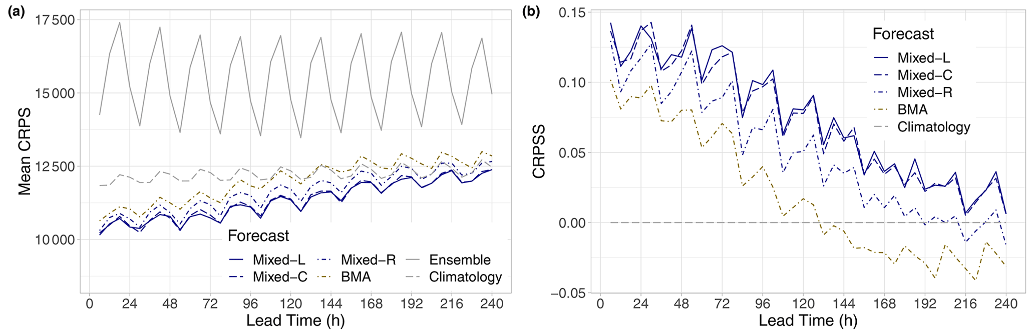
Figure 3 Mean CRPS of post-processed, raw, and climatological visibility forecasts for the calendar year 2021 (a) and CRPSS of post-processed forecasts with respect to climatology (b) as functions of the lead time.

Calibration and sharpness can also be investigated by examining the coverage and average width of $(\mathrm{1}-\mathit{\alpha })\mathrm{100}\mathit{\%},\mathit{\alpha }\in ]\mathrm{0},\mathrm{1}[$, central prediction intervals (intervals between the lower and upper $\mathit{\alpha }/\mathrm{2}$ quantiles of the predictive distribution). Coverage is defined as the proportion of validating observations located in this interval, and, for a properly calibrated predictive distribution, this value should be around (1−α)100 %. Note that level α is usually chosen to match the nominal coverage of $(K-\mathrm{1})/(K+\mathrm{1})\mathrm{100}\mathit{\%}$ of a K-member ensemble, which allows a direct comparison with the raw forecasts.

Further simple tools for assessing the calibration of probabilistic forecasts are the verification rank histogram (or Talagrand diagram) of ensemble predictions and the probability integral transform (PIT) histogram of forecasts given in the form of predictive distributions. The Talagrand diagram is the histogram of the ranks of the verifying observations with respect to the corresponding ensemble forecasts (see, e.g. Wilks, 2019, Sect. 9.7.1), and, in the case of a properly calibrated K-member ensemble, the verification ranks should be uniformly distributed on $\mathit{\{}\mathrm{1},\mathrm{2},\mathrm{\dots },K+\mathrm{1}\mathit{\}}$. The PIT is the value of the predictive CDF evaluated for the verifying observation with possible randomization in the points of discontinuity (see, e.g. Wilks, 2019, Sect. 9.5.4). The PIT values of calibrated predictive distributions follow a standard uniform law, and, in this way, the PIT histogram can be considered to be the continuous counterpart of the verification rank histogram.

Furthermore, the mean and the median of the predictive distributions, as well as the ensemble mean and median, can be considered to be point forecasts for the corresponding weather variable. As the former optimizes the root mean squared error (RMSE) while the latter optimizes the mean absolute error (MAE), we use these two scores to evaluate the accuracy of point predictions (Gneiting, 2011).

Finally, some of the skill scores are accompanied by 95 % confidence intervals based on 2000 block bootstrap samples obtained using the stationary bootstrap scheme, with mean block length derived according to Politis and Romano (1994). In this way, one can get insight into the uncertainty in verification scores and the significance of score differences.

4 Case studies

The predictive performance of the novel mixture model introduced in Sect. 3.1 is tested on the two datasets of ECMWF visibility ensemble forecasts and the corresponding observations described in Sect. 2. As a reference, we consider the BMA approach provided in Sect. 3.2, climatological forecasts (observations of a given training period are considered to be a forecast ensemble), and the raw ECMWF ensemble. Both parametric post-processing models require rather a lot of training data to ensure reliable parameter estimation; moreover, seasonal variations in visibility should also be taken into account during the modelling process. In the case of the mixture model, this latter requirement is addressed with the use of the annual base functions (Eq. 2) in the locations of the component distributions. Hence, one can consider long training periods, which, besides regional modelling, allows clustering-based semi-local or even local parameter estimation too. In the following sections, regional, clustering-based semi-local, and local mixture models are referred to as Mixed-R, Mixed-C, and Mixed-L, respectively. In contrast to the mixture model, there is no seasonality included in the BMA predictive distribution; thus, short training periods are preferred, allowing only regional modelling. The BMA models of both Sect. 4.1 and 4.2 are based on 25 d rolling training periods, the lengths of which are a result of detailed data analysis (comparison of various BMA verification scores for a whole calendar year for training periods of 20, 25, 30, 35, and 40 d). Note that this training-period length is identical to the one suggested by Chmielecki and Raftery (2011). Furthermore, as mentioned, for both calibration approaches, separate modelling is performed for each lead time. Finally, in both case studies, the sizes of the climatological forecasts match the sizes of the corresponding raw ensemble predictions; that is, in Sect. 4.1, observations of 51 d rolling training periods (see Sect. 3.3) are considered, whereas, in Sect. 4.2, climatology is based on 52 past observations.

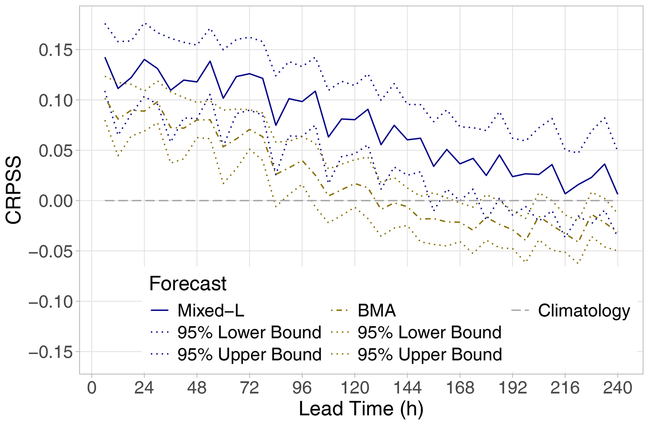
Figure 4 CRPSS with respect to climatology of the best-performing mixed model and the BMA approach (together with 95 % confidence intervals) for the calendar year 2021 as functions of the lead time.

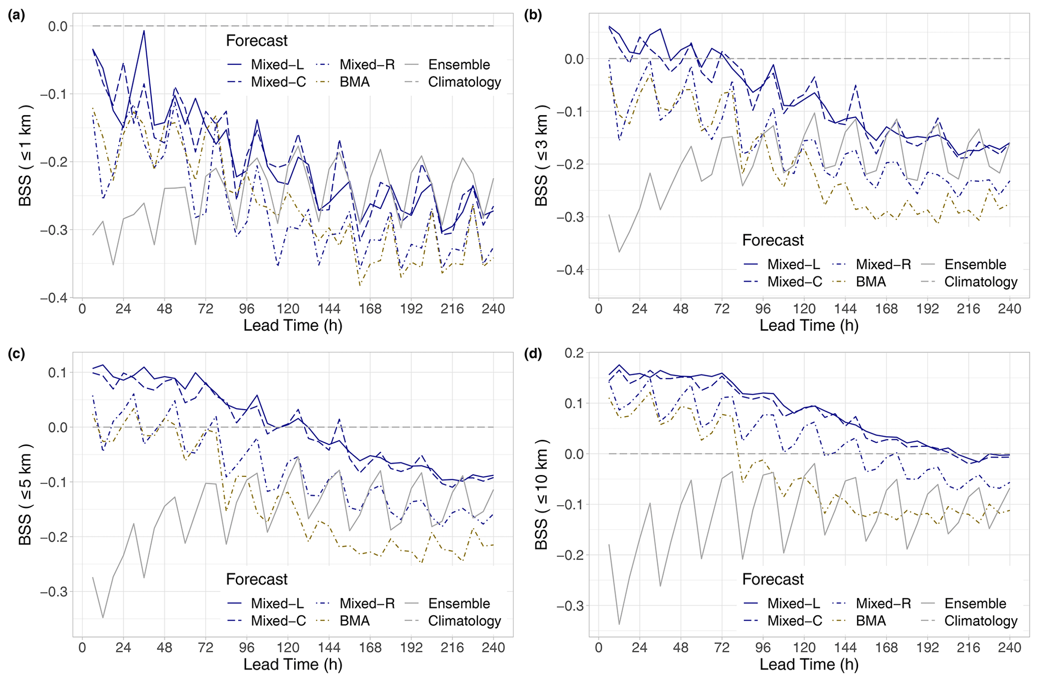
Figure 5 BSS of raw and post-processed visibility forecasts for the calendar year 2021 with respect to climatology for thresholds of 1 km (a), 3 km (b), 5 km (c), and 10 km (d) as functions of the lead time.

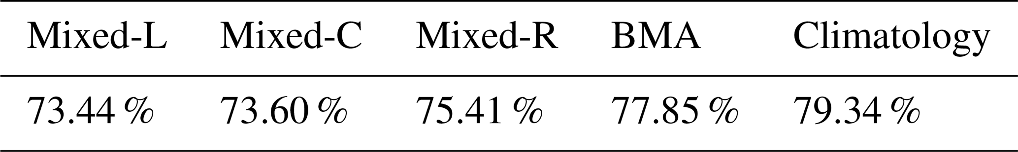
Table 2 Overall mean CRPS of post-processed and climatological visibility forecasts for the calendar year 2021 as a proportion of the mean CRPS of the raw ECMWF ensemble.

4.1 Model performance for 51-member visibility ensemble forecasts

In this case study, the predictive performances of the competing forecasts are compared using data of the calendar year 2021. For the 51-member ECMWF ensemble (control forecast and 50 exchangeable members), the mixture model has 15 free parameters to be estimated, and the comparison of the forecast skill of regional models based on training periods with lengths of 100, 150, … , 350 d reveals that the longest considered training period results in the best predictive performance. This 350 d training window is also kept for local and semi-local modelling, where the 13 locations are grouped into six clusters. Semi-local models with three, four, and five clusters have also been tested; however, these models slightly underperform compared to the chosen one. Furthermore, as mentioned, the 11 parameters of the BMA model are estimated regionally using 25 d rolling training periods, which means a total of 325 forecast cases for each training step. Hence, the data-to-parameter ratio of the regional BMA approach ($\mathrm{325}/\mathrm{11}=\mathrm{29.5}$) is slightly above the corresponding ratio of the local mixture model ($\mathrm{350}/\mathrm{15}=\mathrm{23.3}$). Note that, in this case study, validating visibility observations are reported up to 75 km; hence, the support of all investigated post-processing models is limited to the 0–75 km interval with a point mass at the upper bound.

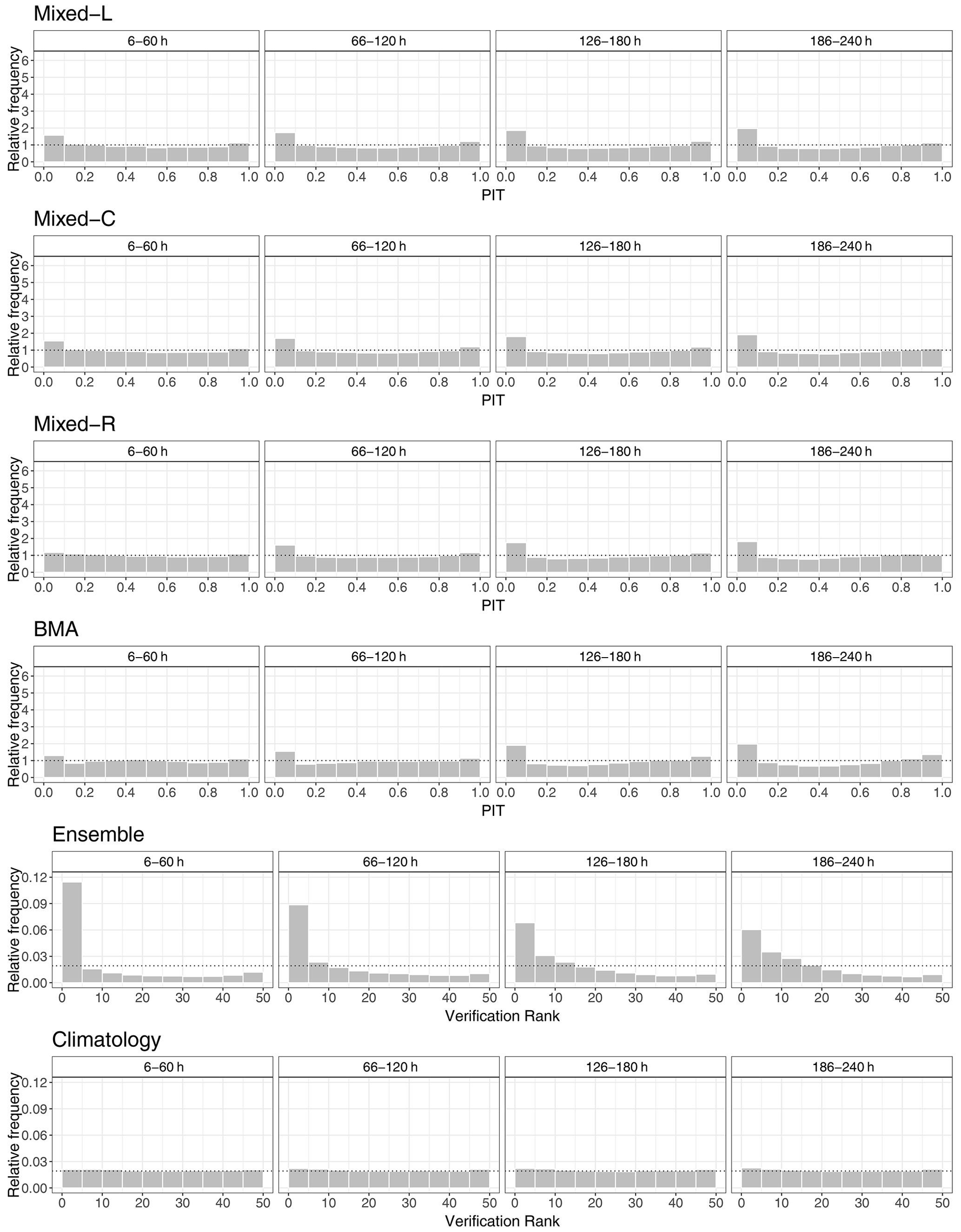
Figure 6 PIT histograms of post-processed and verification rank histograms of climatological and raw visibility forecasts for the calendar year 2021 for lead times of 6–60, 66–120, 126–180, and 186–240 h.

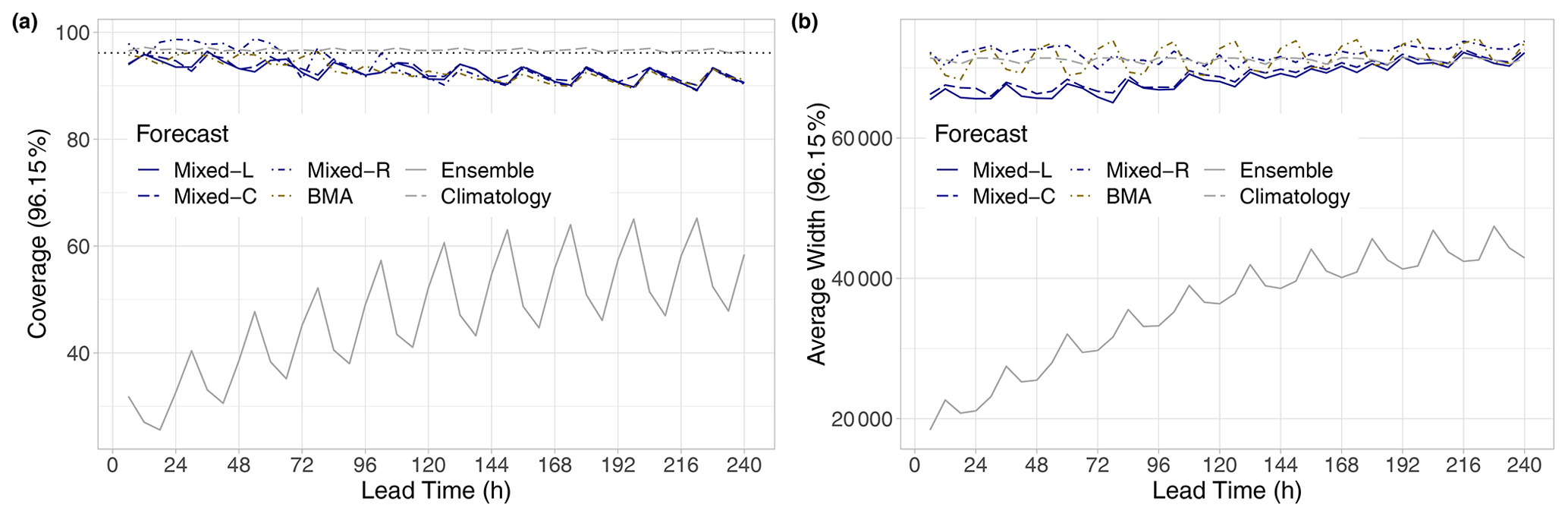
Figure 7 Coverage (a) and average width (b) of nominal 96.15 % central prediction intervals of raw and post-processed visibility forecasts for the calendar year 2021 as functions of the lead time. In panel (a), the ideal coverage is indicated by the horizontal dotted line.

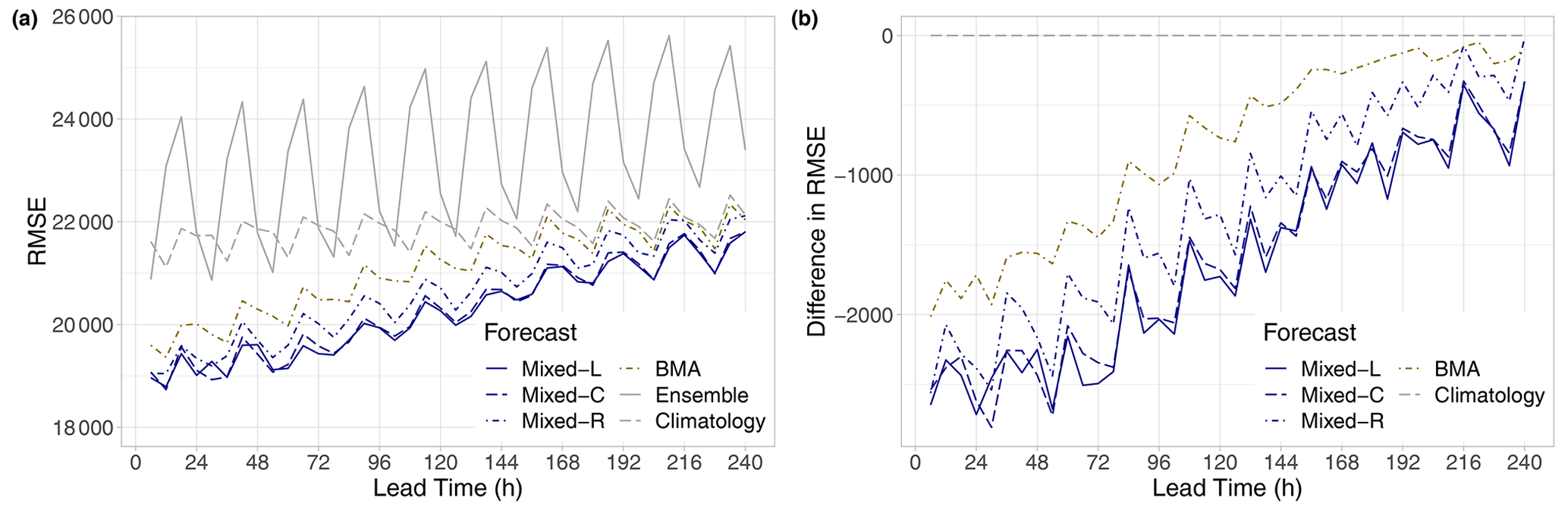
Figure 8 RMSE of the mean forecasts for the calendar year 2021 (a) and difference in RMSE compared to climatology (b) as functions of the lead time.

Figure 3a indicates that, in terms of the mean CRPS, all investigated forecasts considerably outperform the raw visibility ensemble. Note that the clearly recognizable oscillation in the CRPS can be explained by the four different observation times per day, and the raw ensemble exhibits the strongest dependence on the time of the day, having the highest skill at 06:00 UTC. Parametric models are superior to climatology only for shorter forecast horizons, and their advantage gradually fades with the increase in the lead time. The difference between post-processed forecasts and climatology is more visible in the CRPSS values of Fig. 3b. Skill scores of the locally and semi-locally trained mixture models are positive for all lead times, and the difference between these forecasts is negligible. Up to 192 h, the Mixed-R approach also outperforms climatology, and it is clearly ahead of the BMA, which results in positive CRPSS values only for shorter forecast horizons (6–126 h). This ranking of the competing methods is also confirmed by Table 2, providing the overall mean CRPS values of calibrated and climatological forecasts as proportions of the mean CRPS of the raw ECMWF visibility ensemble. We remark that a similarly good performance in terms of climatology with respect to raw and BMA post-processed visibility forecasts of the University of Washington mesoscale ensemble was observed by Chmielecki and Raftery (2011).

In Fig. 4, the CRPSS values of the best-performing locally trained mixture model are accompanied by 95 % confidence intervals, which helps in assessing the significance of the differences in CRPS. The superiority of the Mixed-L forecast over climatology in terms of the mean CRPS is significant at a 5 % level up to 150 h, and between 42 and 174 h, it significantly outperforms the BMA model as well. We remark that, for the latter approach, after 96 h, the CRPSS with respect to climatology fails to be significantly positive (not shown).

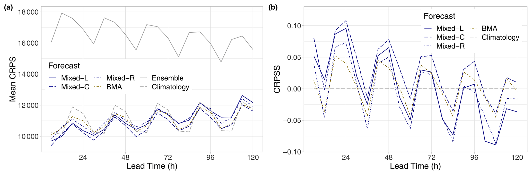
Figure 9 Mean CRPS of post-processed, raw, and climatological EUPPBench visibility forecasts for the calendar year 2018 (a) and CRPSS of post-processed forecasts with respect to climatology (b) as functions of the lead time.

The analysis of the Brier skill scores plotted in Fig. 5 slightly tones the picture of the performance of post-processed forecasts. For visibility not exceeding 1 km, none of the competitors outperform climatology (Fig. 5a), and calibrated predictions are superior to raw ensemble forecasts only for short lead times. With the increase in the threshold, the positive effect of post-processing is getting more and more pronounced, and the ranking of the different models starts matching the one based on the mean CRPS. From the competing calibration methods, the locally and semi-locally trained mixed models consistently display the highest skill, and, for the largest threshold value of 10 km, they outperform climatology up to 204 h (Fig. 5d).

The verification rank and PIT histograms of Fig. 6 again illustrate the primacy of climatology over the raw ensemble and the improved calibration of post-processed forecasts. Raw ECMWF visibility forecasts are under-dispersive and tend to overestimate the observed visibility; however, these deficiencies improve with the increase in the forecast horizon. Climatology results in almost-uniform rank histograms with just a minor under-dispersion, and there is no visible dependence on the forecast horizon. Unfortunately, none of the four investigated post-processing models can completely eliminate the bias of the raw visibility forecasts, which is slightly more pronounced for longer lead times.

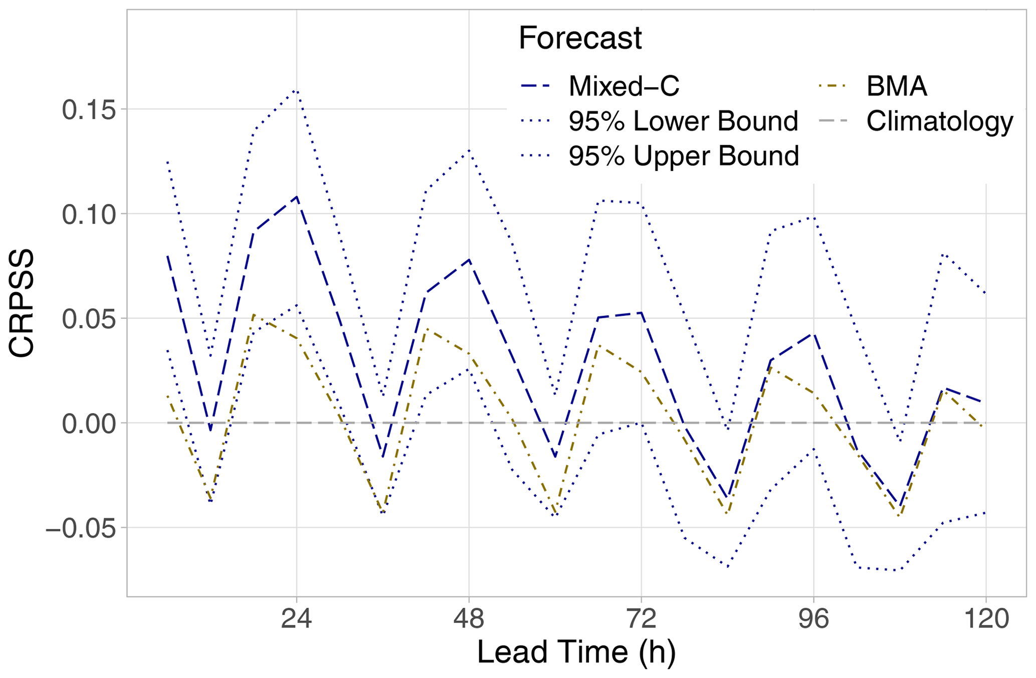
Figure 10 CRPSS with respect to climatology of the best-performing mixed model (together with 95 % confidence intervals) and the BMA approach for the calendar year 2018 as functions of the lead time.

Furthermore, the coverage values of the nominal 96.15 % central prediction intervals depicted in Fig. 7a are fairly consistent with the shapes of the corresponding verification rank and PIT histograms. The under-dispersion of the raw ensemble is confirmed by its low coverage, which shows an increasing trend and a clear diurnal cycle and ranges from 25.58 % to 65.21 %. As one can observe from the corresponding curve of Fig. 7b, the improvement of the ensemble coverage with the increase in the forecast horizon is a consequence of the increase in spread, which results in expanding central prediction intervals. The price of the almost-perfect coverage of climatology with a mean absolute deviation from the nominal value of 0.53 % is the much wider central prediction interval. The coverage values of post-processed forecasts decrease with the increase in the lead time; the corresponding mean absolute deviations from the nominal 96.15 % are 3.55 % (Mixed-L), 3.21 % (Mixed-C), 3.55 % (Mixed-R), and 3.39 % (BMA). However, this negative trend in coverage, especially in the case of the locally and semi-locally trained mixed models, is combined with increasing average width, which can be a consequence of the growing bias.

Finally, in terms of the RMSE of the mean forecast, all post-processing approaches outperform both the raw ensemble and the climatology for all lead times (see Fig. 8a); however, their advantage over climatology is negatively correlated with the forecast horizon. Mixed-L and Mixed-C approaches result in the lowest RMSE values, followed by the Mixed-R and BMA forecasts (see also Fig. 8b), the order of which perfectly matches the ranking based on the mean CRPS (Fig. 3b) and the mean BS for all studied thresholds (Fig. 5).

4.2 Model performance for EUPPBench visibility ensemble forecasts

Since, in the EUPPBench benchmark dataset, the 51-member ECMWF ensemble forecast is augmented with the deterministic high-resolution prediction, the mixture model (Eq. 1) has 17 free parameters to be estimated, whereas, for the BMA predictive PDF (Eq. 3), the parameter vector is 16-D. As mentioned, BMA modelling is based on 25 d regional training, while, to determine the optimal training-period length for mixed models, we again compare the skill of the regionally estimated forecasts based on rolling training windows of 100, 150, …, 350 d. In the case of the EUPPBench visibility data, the skill of the different models is compared with the help of forecast–observation pairs for the calendar year 2018. In contrast to the previous case study, where the longest tested training period of 350 d is preferred, here, the 100 d window results in the best overall performance. Using the same training-period length, we again investigate local modelling and semi-local estimation based on four clusters. Taking into account the maximal reported visibility observation in the EUPPBench benchmark dataset, now the mixed and BMA predictive distributions have point masses at 70 km.

Table 3 Overall mean CRPS of post-processed and climatological EUPPBench visibility forecasts for the calendar year 2018 as a proportion of the mean CRPS of the raw ECMWF ensemble.

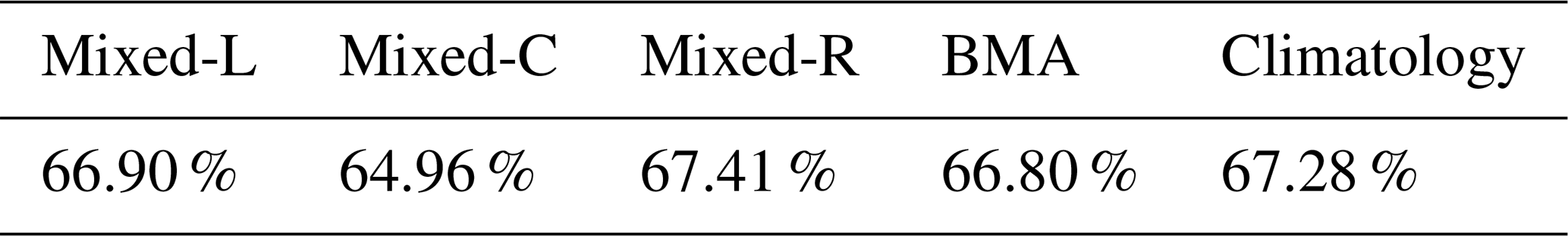
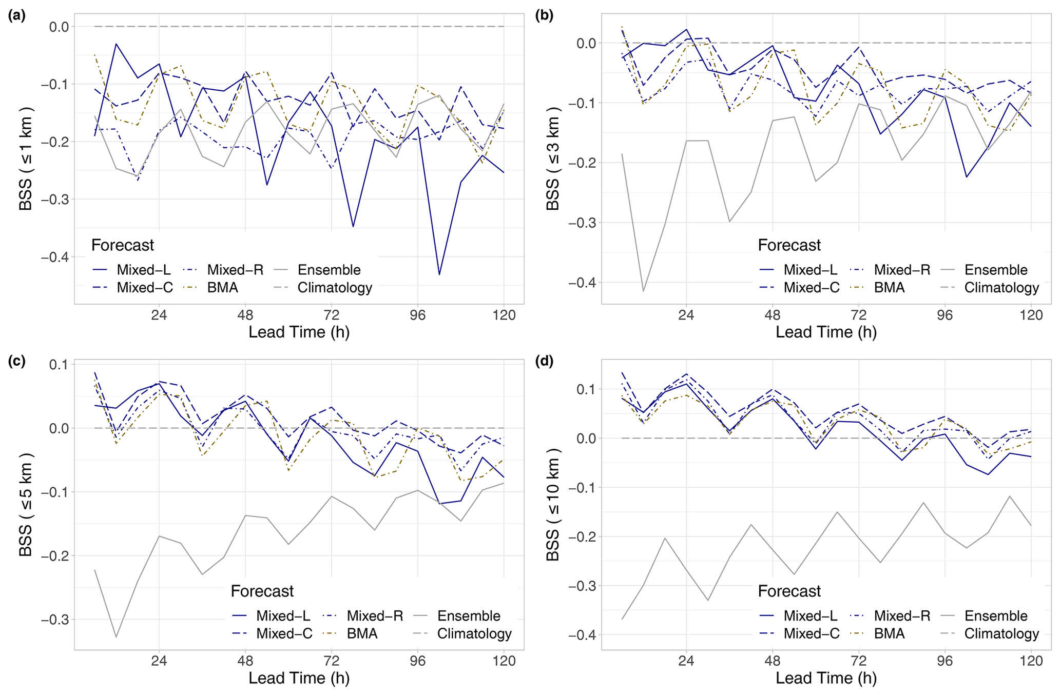
Figure 11 BSS of raw and post-processed EUPPBench visibility forecasts for the calendar year 2018 with respect to climatology for thresholds of 1 km (a), 3 km (b), 5 km (c), and 10 km (d) as functions of the lead time.

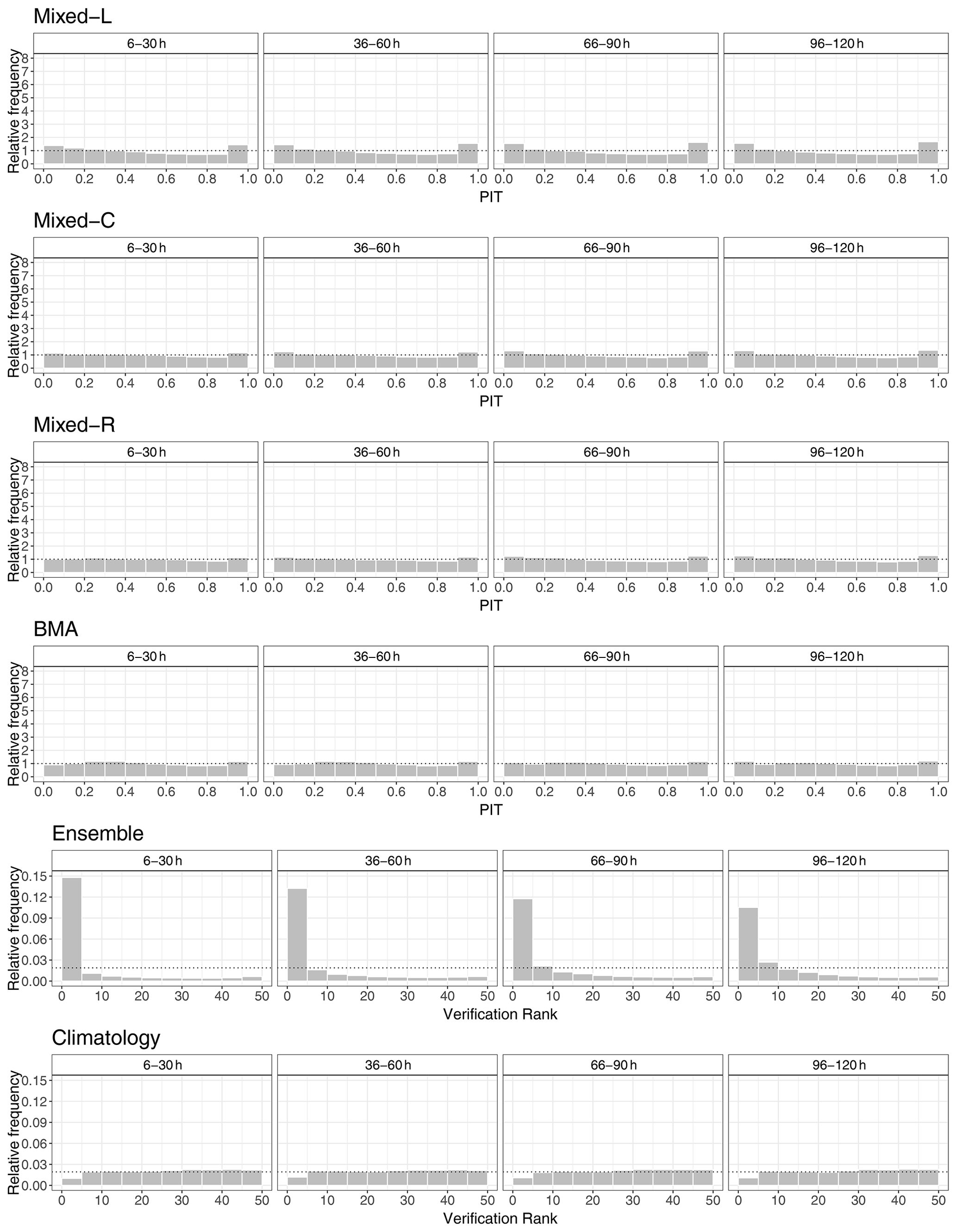
Figure 12 PIT histograms of post-processed and verification rank histograms of climatological and raw EUPPBench visibility forecasts for the calendar year 2018 for lead times of 6–30, 36–60, 66–90, and 96–120 h.

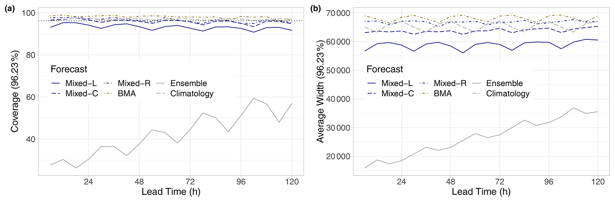
Figure 13 Coverage (a) and average widths (b) of nominal 96.23 % central prediction intervals of raw and post-processed EUPPBench visibility forecasts for the calendar year 2018 as functions of the lead time. In panel (a), the ideal coverage is indicated by the horizontal dotted line.

Again, Fig. 9a shows the mean CRPS of post-processed, raw, and climatological EUPPBench visibility forecasts as functions of the lead time, while in Fig. 9b, the CRPSS values of the mixed and BMA models with respect to the 52 d climatology are plotted. Similarly to the case study of Sect. 4.1, climatological and post-processed forecasts outperform the raw ensemble by a wide margin; however, now the advantage of post-processing over climatology is not so obvious, and the ranking of the calibration methods also differs. From the four investigated models, the Mixed-C model results in the lowest mean CRPS for all lead times but 12 h; nevertheless, even this approach shows negative skill against climatology for lead times corresponding to 12:00 UTC observations. Local modelling (Mixed-L) is competitive only for short forecast horizons, which might be explained by the short training period leading to numerical issues during parameter estimation due to the low data-to-parameter ratio. In general, the skill scores of all post-processing methods show a decreasing trend, with the BMA having the mildest slope. Based on Table 3, providing the improvement in the overall mean CRPS over the raw ECMWF ensemble, one can establish a ranking of Mixed-C – BMA – Mixed-L – Climatology – Mixed-R. Note that the improvements provided here are much larger than the ones in Table 2. In terms of the mean CRPS, the 52-member EUPPBench visibility forecasts are behind the more recent 51-member ensemble predictions studied in Sect. 4.1. This dissimilarity in forecast performance is most likely due to the consecutive improvement in the ECMWF IFS; however, it might also be related to the difference in the forecast domains (see Fig. 1).

Furthermore, according to Fig. 10, even for 00:00, 06:00, and 18:00 UTC observations, the advantage of the best-performing Mixed-C model over climatology is significant at a 5 % level only up to 48 h, whereas the difference in skill from the BMA approach is significant at 6, 24, and 30 h only. Note that the CRPSS of the BMA model with respect to climatology is significantly positive at 5 % only for lead times of 18, 24, 40, and 48 h (not shown).

The Brier skill scores of Fig. 11 lead us to similar conclusions as in the previous case study. For the lowest threshold of 1 km, all forecasts underperform in relation to climatology (Fig. 11a); however, the skill of post-processed predictions improves when the threshold is increased. For the 3, 5, and 10 km thresholds, the ranking of the various models is again identical to the ordering based on the mean CRPS (see Fig. 9b), with the Mixed-C approach exhibiting the best overall predictive performance, closely followed by the BMA model. For the largest threshold of 10 km, up to 54 h, climatology is outperformed even by the least skilful Mixed-L approach (see Fig. 11d), whereas the leading semi-locally trained mixed model results in a positive BSS up to 102 h.

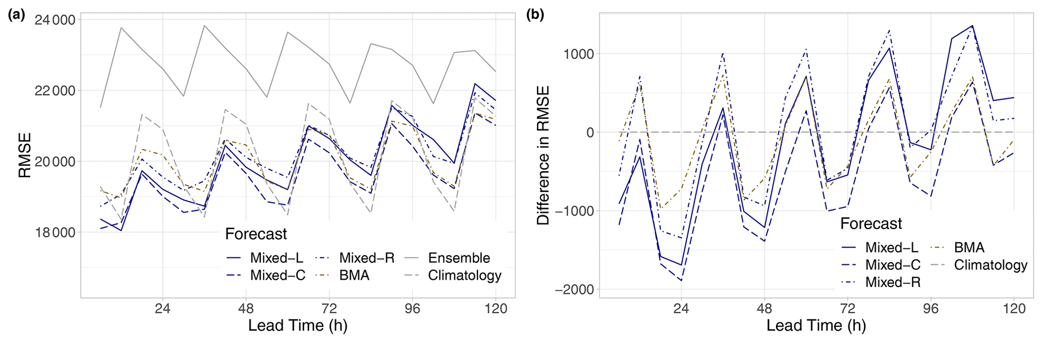
Figure 14 RMSE of the mean EUPPBench forecasts for the calendar year 2018 (a) and difference in RMSE compared to climatology (b) as functions of the lead time.

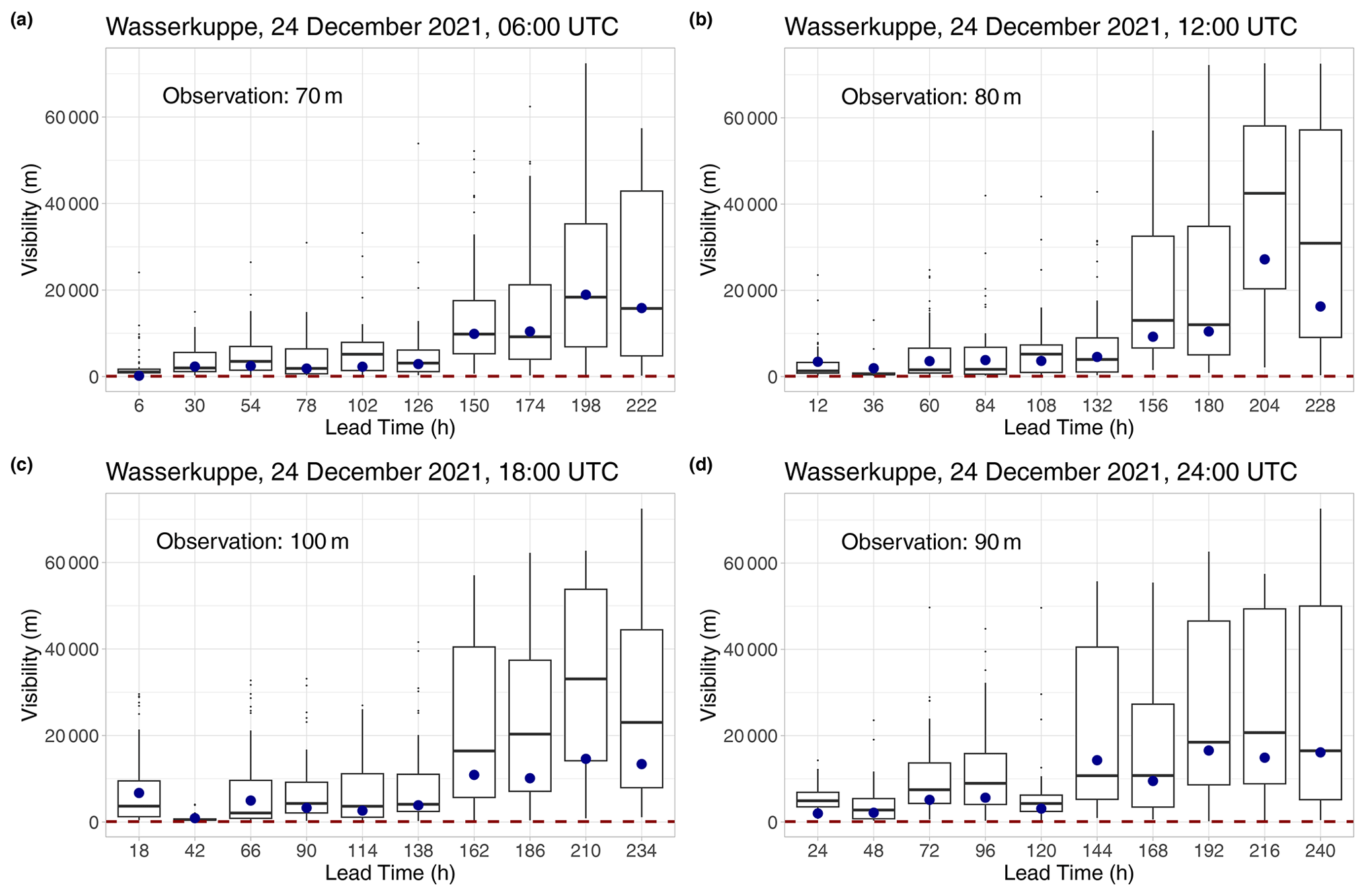
Figure 15 Boxplots of visibility forecasts of various lead times for Wasserkuppe mountain (Germany) for 06:00 UTC (a), 12:00 UTC (b), 18:00 UTC (c), and 24:00 UTC on Christmas Eve of 2021, together with the median forecasts of the Mixed-L model. The observed visibility is indicated by the horizontal dashed line, and the dots denote the Mixed-L medians.

The verification rank histograms of the raw EUPPBench visibility forecasts depicted in Fig. 12 show a much stronger bias than the corresponding panel of Fig. 6, while the improvement with the increase in the forecast horizon is less pronounced. Climatology is also slightly biased but in the opposite direction, whereas the verification rank histograms of all post-processed forecasts are closer to the desired uniform distribution than in the case study of Sect. 4.1. Here the locally trained mixed model exhibits the strongest bias; however, neither the verification rank histograms of climatology nor the PIT histograms of the calibrated forecasts indicate a visible dependence on the forecast horizon.

The fair calibration of climatological and post-processed forecasts can also be observed in Fig. 13a, displaying the coverage values of the nominal 96.23 % central prediction intervals. Semi-locally and regionally trained mixed models and climatology result in almost perfect coverage, closely followed by the BMA model; the corresponding mean absolute deviations from the nominal value are 0.69 %, 0.90 %, 0.72 %, and 1.81 %. The Mixed-L model is slightly behind its competitors, with a mean absolute deviation of 3.00 %, whereas the maximal coverage of the raw EUPPBench ensemble does not reach 60 %. Note that the ranking of the various predictions, the increasing coverage of the raw ensemble, and the lack of a visible trend in the coverage values of post-processed forecasts and climatology are pretty much in line with the shapes of the corresponding histograms of Fig. 12. In general, the average widths of the investigated 96.13 % central prediction intervals (Fig. 13b) are rather consistent with the matching coverage values. Nevertheless, one should remark that the best-performing Mixed-C model results in sharper predictions than climatology and the Mixed-R and BMA approaches.

Finally, according to Fig. 14, in terms of the RMSE of the mean, we see a similar behaviour and ranking of the different forecasts as in the case of the mean CRPS (see Fig. 9), while the raw ensemble is clearly behind the other forecasts, with the increase in the lead time climatology becoming more and more competitive, especially at forecast horizons corresponding to 12:00 UTC observations. However, up to 30 h, both locally and semi-locally trained mixed models result in a lower RMSE than the climatological forecast, and the Mixed-C approach consistently outperforms all other calibration methods for all lead times but 12 h.

5 Conclusions

We propose a novel parametric approach to calibrating visibility ensemble forecasts, where the predictive distribution is a mixture of a gamma and a truncated normal law, both right censored at the maximal reported visibility. Three model variants that differ in the spatial selection of training data are evaluated in two case studies, where, as a reference post-processing method, we consider the BMA model of Chmielecki and Raftery (2011); however, we also investigate the skill of climatological and raw ensemble forecasts. While both case studies are based on ECMWF visibility predictions with a 6 h temporal resolution, they cover distinct geographical regions and time intervals, and only one of them uses the deterministic high-resolution forecast. The results presented in Sect. 4 indicate that all post-processing models consistently outperform the raw ensemble by a wide margin, and the real question is whether statistical calibration results in improvement compared to climatology. In the case of the 51-member operational ECMWF ensemble, e.g. in terms of the mean CRPS of the probabilistic forecast and the RMSE of the mean forecasts, the best-performing locally and semi-locally trained mixed models outperform climatological predictions for all investigated lead times. For the EUPPBench dataset, the situation is far from being so obvious; post-processing can result in consistently positive skill with respect to climatology only up to 30 h. In general, the advantage of post-processed forecasts over climatology shows a decreasing trend with the increase in the forecast horizon, locally and semi-locally trained mixed models are preferred compared to the regionally estimated one, and the BMA approach is slightly behind the competitors.

All in all, the proposed mixed model provides a powerful tool for improving continuous visibility forecasts. As an illustration, consider Christmas Eve of 2021 at the Wasserkuppe mountain in Germany. The visibility was, at most, 100 m during the whole day. According to Fig. 15, in most of the reported forecast cases, the median of the best-performing Mixed-L approach had a smaller absolute error than the ensemble median, and the same applies for the corresponding mean forecasts (not shown).

Note that the general conclusions about the effect of post-processing and the behaviour and ranking of the raw, climatological, and calibrated visibility forecasts are almost completely in line with the results of Baran and Lakatos (2023), where classification-based discrete post-processing of visibility is studied based on extended versions of the current visibility datasets (more observation stations from the same geographical regions). However, there is an essential difference between the approach of Baran and Lakatos (2023) and the models investigated here. In the earlier study, visibility is considered to be a discrete quantity reported in the following values:

$$\begin{array}{ll}{\displaystyle }\mathcal{Y}=\mathit{\{}\mathrm{0},& {\displaystyle }\mathrm{100},\mathrm{200},\mathrm{\dots },\mathrm{4900},\mathrm{5000},\mathrm{6000},\mathrm{7000},\mathrm{\dots },\\ {\displaystyle }& {\displaystyle }\mathrm{29}\mathrm{000},\mathrm{30}\mathrm{000},\mathrm{35}\mathrm{000},\mathrm{40}\mathrm{000},\mathrm{\dots },\mathrm{65}\mathrm{000},\mathrm{70}\mathrm{000}\mathit{\}},\end{array}$$

which reduces post-processing to a classification problem resulting in predictive distributions that form probability mass functions (PMFs) on  𝒴.  Here, we model visibility as a continuous variable, which allows much finer predictions and calculations of the probabilities of various events (e.g. visibility is between 120 and 180 m). Naturally, with the help of a predictive CDF, one can easily create a PMF on 𝒴; thus, both the presented mixed models and the BMA approach of Chmielecki and Raftery (2011) generalize the classification-based discrete post-processing.

The results of this study suggest several further directions for future research. One possible option is to consider a matching distributional regression network (DRN) model, where the link functions connecting the parameters of the mixture predictive distribution with the ensemble forecast are replaced by an appropriate neural network. This parametric machine-learning-based approach has proved to be successful for several weather quantities, such as temperature (Rasp and Lerch, 2018), precipitation (Ghazvinian et al., 2021), wind gust (Schultz and Lerch, 2022), wind speed (Baran and Baran, 2021), or solar irradiance (Baran and Baran, 2024).

Furthermore, one can also investigate the impact of the introduction of additional covariates on the forecast skill of parametric models based on the proposed predictive distribution of censored gamma–truncated and censored normal mixtures. In the DRN setup, this step is rather straightforward and might result in significant improvement in predictive performance (see, e.g Rasp and Lerch, 2018; Schultz and Lerch, 2022). A natural choice can be any further visibility forecast (for instance, the one of the Copernicus Atmospheric Monitoring Service); however, forecasts of other weather quantities affecting visibility can also be considered.

Finally, using two-step multivariate post-processing techniques, one can extend the proposed mixture model to obtain spatially and/or temporally consistent calibrated visibility forecasts. For an overview of the state-of-the-art multivariate approaches, we refer the reader to Lerch et al. (2020) and Lakatos et al. (2023).