Spatiotemporal functional permutation tests for comparing observed climate behavior to climate model projections

Comparisons of observed and modeled climate behavior often focus on central tendencies, which overlook other important distributional characteristics related to quantiles and variability. We propose two permutation procedures, standard and stratified, for assessing the accuracy of climate models. Both procedures eliminate the need to model cross-correlations in the data, encouraging their application in a variety of contexts. By making only slightly stronger assumptions, the stratified procedure dramatically strengthens the ability to detect a difference in the distribution of observed and climate model data. The proposed procedures allow researchers to identify potential model deficiencies over space and time for a variety of distributional characteristics, providing a more comprehensive assessment of climate model accuracy, which will hopefully lead to further model refinements. The proposed statistical methodology is applied to temperature data generated by the state-of-the-art North American Coordinated Regional Climate Downscaling Experiment (NA-CORDEX).

1 Introduction

This paper is concerned with the comparison of predictions of commonly used climate models to actual (reanalysis) climate data. Phillips (1956) is credited with introducing the first successful climate model. In the subsequent 60+ years, climate models have grown increasingly more complex and popular for describing climate behavior, particularly for exploring the potential impact of humans on future climate.

Projections of future climate are typically based on general circulation models (GCMs), which are sometimes referred to as global climate models. One way to assess the reliability of a climate model is to examine whether the model is able to reproduce climate behavior observed in the past (Raäisaänen, 2007; Randall et al., 2007; IPCC, 2014; Garrett et al., 2023). The deficiencies a model has in describing observed climate are likely to be amplified in the future and may weaken their usefulness in making decisions based on the available data.

Many comparisons have been made between climate model projections of current climate and historical records. Lee et al. (2019) compare mean near-surface air temperature and precipitation decadal trends from climate models to historical trends over the continental USA. Jia et al. (2019) compute statistics over the Tibetan Plateau (TP) for observational data and various climate models, including the sample mean, standard deviation, root-mean-square error, and time- and space-based correlation coefficients, to assess the accuracy of climate models in describing the behavior of observed data. Kamworapan and Surussavadee (2019) compare 40 GCMs to various observational and reanalysis data sets using 19 performance metrics, including mean annual temperature and precipitation, mean seasonal cycle amplitude of temperature and precipitation, the correlation coefficient between simulated and observed mean temperatures and precipitation, and variance of annual average temperature and precipitation over a 99-year period. Oh et al. (2023) compare the root-mean-square difference (RMSD) and Taylor skill score statistics of 17 climate models with observational data for several variables and two ocean areas. These approaches tend to focus on average behavior over certain time periods and partitions of the study area. They may not be adequate in describing more detailed aspects of behavior over time and space. Methods for evaluating climate models from a functional data perspective are less common. Vissio et al. (2020) proposed using a Wasserstein distance to measure the gap between a climate model and a reference distribution based on raw observations or reanalysis data. Their goal was to rank the “nearness” of various climate model outputs to a reference data set. Garrett et al. (2023) extended this idea to correct for “misalignment” of the time periods of the data sets being compared. We cast the problem of evaluating the agreement of a model with historical records into a statistical testing problem within the framework of functional data analysis. In particular, since we consider whole curves rather than averages, our approach allows us to detect shifts in the seasonal cycle in the GCMs that do not match the observed data. In contrast to the other functional approaches, which seem to focus on ranking the similarity of individual climate model outputs to a reference data set, our goal is to assess whether a reference data set can be viewed as a realization from a hypothetical climate distribution that produced the collection of climate model outputs.

In what follows, we (i) describe a novel testing procedure for spatiotemporal functional data and (ii) provide a complementary case study that expands the types of climate characteristics considered in order to provide a more comprehensive evaluation of how a climate model output compares to observed climate data (or, in our case, a close proxy). We will compare daily temperature data for the fifth generation of the European Centre for Medium-Range Weather Forecasts (Copernicus Climate Change Service (C3S), 2017) to a climate model output provided by the North American Coordinated Regional Climate Downscaling Experiment (NA-CORDEX; Mearns et al., 2017). For convenience, we will refer to these data sets as the ERA5 data and NA-CORDEX data, respectively. Our goal is to assess how well NA-CORDEX climate model projections capture the behavior of the observed climate, as characterized by the ERA5 reanalysis data. In Sect. 2, we describe these data sets in more detail as they directly motivate our methodology. In Sect. 3, we describe the statistical approach for comparing the climate models. In Sect. 4, we perform a simulation study that highlights the benefits of the proposed method over the standard procedure. In Sect. 5, we describe the results of our climate model comparisons. Lastly, we summarize our investigation in Sect. 6.

2 Description of the ERA5 and NA-CORDEX data

2.1 General information about climate reanalysis data

A climate reanalysis feeds large amounts of observational data into data assimilation models to provide a numerical summary of recent climate across much or all of the Earth at regular spatial resolutions and time steps (Dee et al., 2016; European Centre for Medium-Range Weather Forecasts, 2023b). Typically, all available observational data are fed into the data assimilation algorithm at regular hourly intervals (e.g., every 6–12 h) to estimate the state of the climate at each time step (Dee et al., 2016). The resulting data product typically provides information on numerous climate variables such as surface air temperature, total precipitation, and wind speed. A climate reanalysis data product is much more manageable from a research standpoint, since the product is uniform and since the researcher does not need to access the many observational data sets or immense computational resources needed to produce the data (Dee et al., 2016). However, Dee et al. (2016) point out that because climate reanalysis data use many different types of data from different sources, locations, and times, this can result in uncertainty in the estimated climate at each time step and lead to phantom data patterns.

2.2 ERA5 background information

The ERA5 global reanalysis is the fifth-generation reanalysis produced by the European Centre for Medium-Range Weather Forecasts (Hersbach et al., 2017, 2020a) and is made freely available through the Copernicus Climate Change Service Climate Data Store (Copernicus Climate Change Service (C3S), 2017). The reanalysis data are available from January 1940 to approximately the present day. The data assimilate 74 data sources using a 4D‐Var (four-dimensional variational) ensemble data assimilation system (European Centre for Medium-Range Weather Forecasts, 2023a; Hersbach et al., 2020a). The program produces many atmospheric, land, and oceanic climate variables. Our analysis focuses on the monthly average daily maximum near-surface air temperature from the ERA5 hourly data on single levels from 1940 to the present (Hersbach et al., 2020b). Near-surface temperature is the 2 m temperature, which is effectively the temperature that humans experience.

2.3 NA-CORDEX background information

NA-CORDEX is focused on downscaling the climate model output in the North American domain using boundary conditions from the CMIP5 archive (Hurrell et al., 2011). It is part of the broader CORDEX organized by the World Climate Research Programme, which aims to organize regional climate downscaling through partnerships with research groups across the globe (CORDEX, 2020). Figure 1a displays the NA-CORDEX domain with the associated geopolitical boundaries. A regional climate model (RCM) receives boundary conditions from a GCM and predicts (downscales) the resulting climate behavior at a finer spatial scale than the associated GCM, which allows researchers to investigate climate behavior at smaller spatial resolutions (e.g., at the city level instead of county level).

Climate model outputs typically exhibit bias compared to observations. This bias can be corrected using various algorithms by adjusting the data using a reference data set. The NA-CORDEX program used the multivariate bias correction (MBCn) algorithm (Cannon et al., 2015; Cannon, 2016, 2018) to perform this correction. MBCn uses quantile mapping to adjust the statistical distribution of the model output to match the distribution of a reference data set. MBCn makes this adjustment jointly for multiple variables and not only for individual marginal distributions, which is important because climate models produce many variables simultaneously. The NA-CORDEX program bias-corrected the original climate model output using two observational data sets, i.e., Daymet and gridMET. Additional details are discussed by McGinnis and Mearns (2021). Figure 1 displays heat maps of the average temperature (°C) of the raw NA-CORDEX data, as well as the bias added to the raw data for both reference data sets. The Daymet data set includes substantially more spatial locations. All subsequent analyses will be performed on bias-corrected data over the corresponding domain.

The NA-CORDEX utilizes combinations of six different GCMs to provide the boundary conditions for seven different RCMs under two sets of future conditions, though not all combinations are currently available. Our analysis will focus on the monthly average of daily maximum near-surface air temperature from the available combinations.

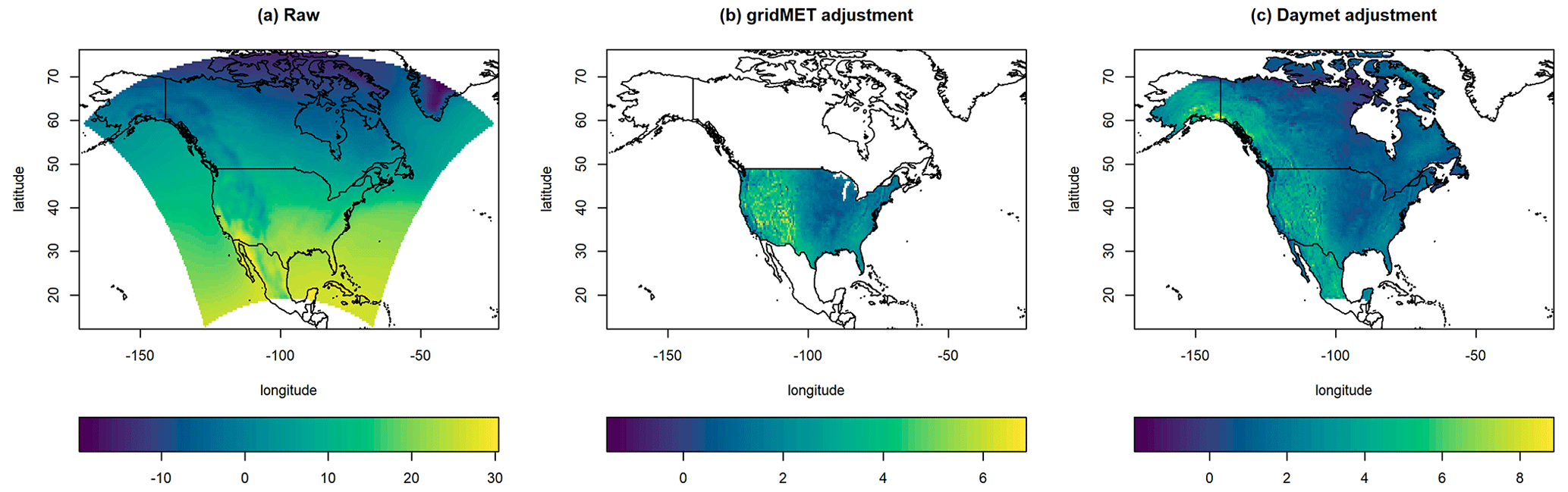
Figure 1 Temperature-related heat maps for the NA-CORDEX data: (a) the average temperature (°C) of the raw NA-CORDEX data from 1950–2004, (b) the temperature bias added to the raw NA-CORDEX data after performing the MBCn bias correction using the gridMET data, and (c) the temperature bias added to the raw NA-CORDEX data after performing the MBCn bias correction using the Daymet data.

2.4 Details on comparing the ERA5 and NA-CORDEX data

The ERA5 data are available at locations across the globe, while the NA-CORDEX data are available in the areas surrounding North America. Consequently, we restrict our use of the ERA5 data to the same subdomain as the NA-CORDEX data. Furthermore, we restrict our analysis to locations over the primary land masses around North America (i.e., not small islands or the sea), as response behavior can change dramatically between land and sea and the spatial resolution may not allow for adequate representation of small land masses. Both ERA5 and NA-CORDEX data sets are available at a common spatial resolution known as 44i. The longitude and latitude locations of 44i data are available in 0.5° increments starting from ±0.25°. The “44” in 44i refers to the fact that locations separated 0.5° in longitude along the Equator are approximately 44 mi (miles) (about 70.8 km) apart.

Additionally, since we have previously noted that variables such as precipitation should be used with extreme caution in the context of reanalysis data, we only consider temperature-related data since they are provided by both the ERA5 and NA-CORDEX programs.

Lastly, our goal is to compare the observed climate to climate model projections. The historical period for the NA-CORDEX data runs from 1950–2005, while the reanalysis data we consider runs from 1940 to the present day. However, there are known issues with temperature in December 2005 for several NA-CORDEX models (NA-CORDEX, 2020), so we restrict our analysis to monthly temperature for the complete years 1950–2004.

For the available data with the above characteristics, there is a single realization of the ERA5 data and 15 realizations of NA-CORDEX data (or, more specifically, 15 combinations of RCM–GCM models with available data). Six RCMs were used to produce the NA-CORDEX data:

• CanRCM4 (Scinocca et al., 2016),

• HIRHAM5 (Christensen et al., 2007),

• QCRCM5 (Martynov et al., 2013; Šeparović et al., 2013),

• RCA4 (Samuelsson et al., 2011),

• RegCM4, (Giorgi and Anyah, 2012), and

• WRF (Skamarock et al., 2008).

Additional details about the RCMs are provided in Table S1 in the Supplement. These RCMs were combined with eight versions of GCMs:

• CanESM2 (Chylek et al., 2011),

• EC-Earth (Hazeleger et al., 2010),

• GEMATM-Can (Hernández-Díaz et al., 2019),

• GEMATM-MPI (Hernández-Díaz et al., 2019),

• GFDL-ESM2M (Dunne et al., 2012),

• HadGEM2-ES (Bellouin et al., 2011),

• MPI-ESM-LR (Giorgetta et al., 2013), and

• MPI-ESM-MR (Giorgetta et al., 2013).

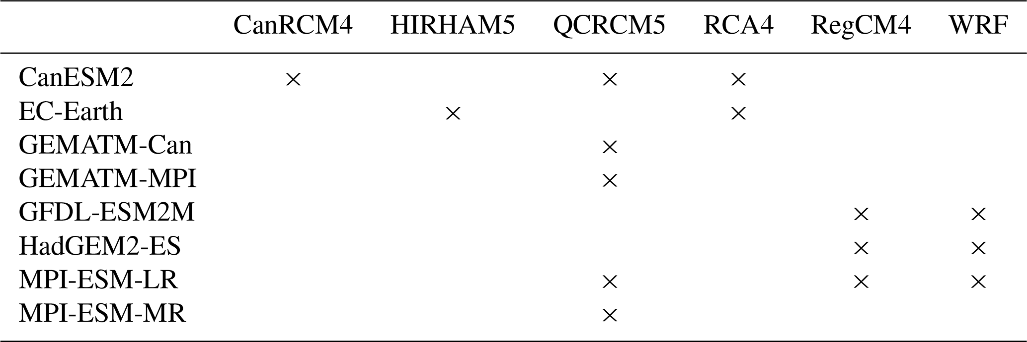
Although there are 48 total RCM–GCM combinations possible, data were created for only 15 combinations. We summarize the 15 RCM–GCM combinations used to produce the data used in this analysis in Table 1.

Table 1 RCM–GCM combinations used to produce the 15 NA-CORDEX data sets used in this paper.

3 Methods

3.1 Testing context

Our goal is to assess how well the NA-CORDEX climate model projections capture the behavior of observed climate using the ERA5 reanalysis data as a proxy. If the climate model projections provide an accurate representation of the observed data, then one can view the observed data as a realization from the same climate distribution producing the NA-CORDEX climate model projections. This will be formalized as the null hypothesis, keeping in mind the usual caveats of the Neyman–Pearson paradigm. The alternative hypothesis will be that the observed data follow a different distribution than the model data. In what follows, we formally describe the problem using appropriate mathematical notation and propose a statistical methodology for making an inference.

The data we consider are viewed as realizations of annual spatiotemporal random fields, i.e., $\mathit{\left\{}{X}_n\right(\mathit{s},t),\mathit{s}\in D,t\in T\mathit{\}}$, where n denotes year, s spatial location, and t time within the year. The spatial domain D⊂ℝ² is assumed to be a known, bounded region. Both the spatial domain and time domain can be continuous, but the data are observed on discrete grids, both in space and time, which will be defined in the following. The year domain $\mathcal{N}\subset {\mathbb{Z}}^{+}$ is assumed to be a known, fixed set of positive integer values. We use the shorthand X_n to denote the spatiotemporal random field in year n, and we use F_n to denote its distribution function. Similarly, we use $X=\mathit{\{}{X}_n,n\in \mathcal{N}\mathit{\}}$ to denote the set of the annual random fields for all years in 𝒩, and we use F to denote the corresponding distribution function. Consider first a fixed year n. The range of the function F_n is [0,1], and its domain is the set of real-valued functions on D×T, which is denoted ℱ(D×T). Thus, $F_n:\mathcal{F}(D\times T)\to [\mathrm{0},\mathrm{1}]$. For $f\in \mathcal{F}(D\times T)$,

$$\begin{array}{rl}& P\left(X_n(\mathit{s},t)\le f(\mathit{s},t),\mathit{s}\in D,t\in T\right)\\ & =F_n\left(f(\mathit{s},t),\mathit{s}\in D,t\in T\right).\end{array}$$

For mathematical consistency, ℱ(D×T) must be a subset of a suitable Hilbert space of measurable functions (Horváth and Kokoszka, 2012, Chap. 2). In our context, we consider two functions for F_n, both unknown. The first one, denoted $F_n^{\mathrm{R}}$, is the distribution function corresponding to real climate, which is represented by the reanalysis data. Thus, the superscript R can be associated with both “real” and “reanalysis”. We observe only one realization from the distribution $F_n^{\mathrm{R}}$. The second distribution function, denoted $F_n^{\mathrm{M}}$, describes data generated by the climate model for year n. We generally have a large number of realizations from this distribution. We say that the model describes real data in year n satisfactorily if we cannot reject the hypothesis $F_n^{\mathrm{R}}=F_n^{\mathrm{M}}$. To evaluate the model over all available years, we work with distribution functions F defined by

$$\begin{array}{}\text{(1)}& \begin{array}{rl}& P\left(X_n(\mathit{s},t)\le f(\mathit{s},t,n),\mathit{s}\in D,t\in T,n\in \mathcal{N}\right)\\ & =F\left(f(\mathit{s},t,n),\mathit{s}\in D,t\in T,n\in \mathcal{N}\right),\end{array}\end{array}$$

where f is a real function over $D\times T\times \mathcal{N}$. We would ideally consider testing

$$\begin{array}{}\text{(2)}& H_{\mathrm{0}}:F^{\mathrm{R}}=F^{\mathrm{M}}\text{versus}{H}_a:F^{\mathrm{R}}\ne F^{\mathrm{M}}.\end{array}$$

Effectively, this is assessing whether X^R could plausibly be viewed as a realization from F^M.

Before describing our approach, we formulate the assumptions we will use. These assumptions must, on the one hand, be realistic but, on the other hand, lead to feasible tests. We use the notation M_j to refer to the jth GCM–RCM combination from the NA-CORDEX program, with $j=\mathrm{1},\mathrm{2},\mathrm{\dots },N_M$, and we use $X^{M_j}$ to denote the spatiotemporal field associated with climate model M_j. In our analysis, N_M=15. We assume that $X^{{\mathrm{M}}_j}\stackrel{\text{i.i.d.}}{\sim }{F}^{\mathrm{M}}$, i.e., that the climate model realizations are independent and identically distributed (i.i.d.). The above assumption is realistic when the model runs use different initial parameters for each run or when model runs come from a different combination of models. The initial parameters are the initial conditions from which an RCM begins its model run. Since the RCMs are programmed differently, their outputs are independent of each other. If different RCMs use the same initial conditions, then the model outputs may present some autocorrelation since they are being forced by the same process. Thus, GCM–RCM combinations that share the same GCM may not satisfy the assumption of independent model runs. We will address this concern in the Supplement.

Additionally, $X_n^{{\mathrm{M}}_j}(\mathit{s},t)$ denotes the random variable observed at location s and time t in year n for model combination M_j. To reflect real data like temperature or precipitation (or statistics derived from them), we cannot assume that the random field $\mathit{\left\{}{X}_n\right(\mathit{s},t),s\in D,t\in T\mathit{\}}$ is stationary or Gaussian. We thus do not assume that the X_n fields have the same distribution, so various trends or changes in n are allowed. Independence of errors is commonly assumed in statistical models, and we also assume independence of annual error functions around potential decadal trends or changes. We emphasize that we do not assume spatial or temporal independence within the fields; that is, we do not assume that X_n(s₁,t₁) is independent of X_n(s₂,t₂) if s₁≠s₂ or t₁≠t₂. The annual fields are viewed as functional objects with a complex spatiotemporal dependence structure.

In the context of the ERA5 and NA-CORDEX data, it is reasonable to assume that realizations of X^R and $X^{M_j}$ are observed at identical spatial locations s, time points t, and years n, so we do so in what follows. Let $\mathcal{S}=\mathit{\{}{\mathit{s}}_{\mathrm{1}},\mathrm{\dots },{\mathit{s}}_{N_{\mathit{s}}}\mathit{\}}\subset D$ be the set of observed spatial locations, $\mathcal{T}=\mathit{\{}{t}_{\mathrm{1}},t_{\mathrm{2}},\mathrm{\dots },t_{N_t}\mathit{\}}\subset T$ denote the set of observed time points, and $\mathcal{N}=\mathit{\{}{n}_{\mathrm{1}},n_{\mathrm{2}},\mathrm{\dots },n_{N_n}\mathit{\}}$ denote the set of observed years.

3.2 Tests of equality of distributions

We first consider a test assessing whether the distribution of the reanalysis data matches that of the model data. Formally, we consider the testing problem stated in Eq. (2). We construct the test statistic using the distance between the real and model data values. For a fixed location s and model M_j, set

$$\begin{array}{rl}& D_{R,M_j}\left(\mathit{s}\right)={\displaystyle \frac{\mathrm{1}}{N_n}}{\displaystyle \frac{\mathrm{1}}{N_t}}\sum _{n=\mathrm{1}}^{N_n}\sum _{t=\mathrm{1}}^{N_t}\left|X_n^{\mathrm{R}}(\mathit{s},t)-X_n^{M_j}(\mathit{s},t)\right|,\\ & j=\mathrm{1},\mathrm{2},\mathrm{\dots },N_M.\end{array}$$

The test statistic at location s is

$$\begin{array}{}\text{(3)}& \widehat{T}\left(\mathit{s}\right)={\displaystyle \frac{\mathrm{1}}{\sqrt{N_M}}}\sum _{j=\mathrm{1}}^{N_M}{D}_{R,M_j}\left(\mathit{s}\right).\end{array}$$

We can avoid the problem of multiple testing by considering the distance over the whole space; that is,

$$\begin{array}{ll}{\displaystyle }{D}_{R,M_j}& {\displaystyle }={\displaystyle \frac{\mathrm{1}}{N_s}}{\displaystyle \frac{\mathrm{1}}{N_n}}{\displaystyle \frac{\mathrm{1}}{N_t}}\sum _{\mathit{s}\in \mathcal{S}}\sum _{n=\mathrm{1}}^{N_n}\sum _{t=\mathrm{1}}^{N_t}\left|X_n^{\mathrm{R}}(\mathit{s},t)-X_n^{M_j}(\mathit{s},t)\right|,\\ {\displaystyle }& {\displaystyle }={\displaystyle \frac{\mathrm{1}}{N_{\mathbf{s}}}}\sum _{\mathit{s}\in \mathcal{S}}{D}_{R,M_j}\left(\mathbf{s}\right),j=\mathrm{1},\mathrm{2},\mathrm{\dots },N_M.\end{array}$$

The global test statistic is then

$$\begin{array}{}\text{(4)}& \widehat{T}={\displaystyle \frac{\mathrm{1}}{\sqrt{N_M}}}\sum _{j=\mathrm{1}}^{N_M}{D}_{R,M_j}.\end{array}$$

We explain the approximation of the null distribution in Sect. 3.4.1 and 3.4.2.

While the statistic in Eq. (4) solves the problem of multiple testing, the information that can be drawn from the test based on it is limited; if the null hypothesis is rejected, the test does not indicate over which spatial regions the differences occur and which characteristics contribute to them. These issues are addressed in the following sections.

3.3 Distributional characteristics

As noted above, testing the equality of distributions is useful, but such tests do not indicate how the distributions differ if the null hypothesis is rejected. We therefore also propose tests to assess whether certain characteristics of F^R (e.g., related to center, dispersion, skewness, and extremes) are consistent with the same characteristics of F^M. In this section, we define the characteristics we consider as population parameters and introduce their estimators. Recall that $X_n^{\mathrm{M}}(\mathit{s},t)$ is the value of a scalar random field indexed by n,s, and t. For a fixed s, we have a scalar random field indexed by n and t. This random field has an expected value (a real number) which we denote by μ^M(s). We estimate it by

$${\widehat{\mathit{\mu }}}^{\mathrm{M}}\left(\mathit{s}\right)={\displaystyle \frac{\mathrm{1}}{N_M{N}_n{N}_t}}\sum _{j=\mathrm{1}}^{N_M}\sum _{n\in \mathcal{N}}\sum _{t\in \mathcal{T}}{X}_n^{M_j}(\mathit{s},t).$$

The expected value μ^M(s) ignores any possible changes in the mean between years or within a year but varies with spatial location.

Naturally, we could consider other central tendency characteristics such as the median; dispersion characteristics such as the standard deviation, interquartile range, or total range; or more extremal characteristics such as the 0.025 or 0.975 quantiles, though special care must be taken to ensure that these characteristics are well-defined. These characteristics may not be defined over space, time, or year domains because of trends or other factors. They are to be interpreted as parameters of the populations of all, infinitely many, model or real data replications for a fixed spatiotemporal domain. One may, for example, consider the 0.05 quantile function of the model distribution defined by

$$\begin{array}{rl}{q}_{\mathrm{0.05}}& =inf\mathit{\{}x\in \mathbb{R}:P(X_n(\mathit{s},t)\ge x,\mathit{s}\in D,t\in T,\\ & n\in \mathcal{N})\ge \mathrm{0.95}\mathit{\}}.\end{array}$$

Within the context described above, in addition to the hypotheses in Eq. (2), we may test more specific hypotheses of the general form

$$\begin{array}{}\text{(5)}& H_{\mathrm{0}}:{\mathit{\theta }}^{\mathrm{R}}={\mathit{\theta }}^{\mathrm{M}}\text{versus}{H}_a:{\mathit{\theta }}^{\mathrm{R}}\ne {\mathit{\theta }}^{\mathrm{M}},\end{array}$$

assuming that the parameter is well-defined, which allows us to assess the ways in which the distributions of F^M and F^R might differ. For example, while the means may be similar, the dispersion may differ. In Sect. 3.4, we discuss how the tests are practically implemented.

3.4 Permutation tests

In this section, we propose solutions to the testing problems in Eqs. (2) and (5). In Sect. 3.4.1, we explain how standard permutation tests can be applied, and we discuss their drawbacks. Section 3.4.2 focuses on an approach we propose to construct useful tests.

3.4.1 Standard permutation tests

First introduced by Fisher (1935), permutation tests are a popular approach for hypothesis tests comparing characteristics of two (or more) groups while requiring minimal distributional assumptions. In contrast to parametric tests, the weakened assumptions typically come at the expense of greater computational effort. Instead of assuming that the null distribution can be approximated by a parametric distribution, the null distribution is approximated using a resampling procedure. Specifically, the responses are permuted for all observations that are exchangeable under the null hypothesis, and a relevant test statistic quantifying the discrepancy between the relevant groups is computed for the permuted data. The null distribution is determined by considering the empirical distribution of the statistics computed for all possible permutations of the data (or approximated if a subset of all permutations is used). A statistical decision is made by comparing the observed statistic to the empirical distribution and quantifying the associated p value. Good (2006) provides details of the theory and practice of permutation tests.

The use of permutation tests in the framework of functional data seems to have been introduced by Holmes et al. (1996) for comparing functional brain-mapping images and has been developed in many directions; see Nichols and Holmes (2002), Reiss et al. (2010), Corain et al. (2014), and Bugni and Horowitz (2021), among many others. These tests assume that the functions in two or more samples are i.i.d. or form i.i.d. regressor–response pairs. As explained above, this is not the case in the context of spatiotemporal functions we consider. We now elaborate on the potential application of permutation tests in our framework.

Let $\mathbf{X}=\mathit{\{}{X}^{{\mathrm{R}}_{\mathrm{1}}},\mathrm{\dots },X^{{\mathrm{R}}_{N_R}},X^{{\mathrm{M}}_{\mathrm{1}}},\mathrm{\dots },X^{{\mathrm{M}}_{N_M}}\mathit{\}}$ denote the observed data, where (motivated by our application) the superscripts R and M denote responses from two different groups and where N_R and N_M denote the number of observations in each group. Let T(X) denote a statistic for assessing whether θ^R=θ^M. Let $T\left({\stackrel{\mathrm{̃}}{\mathbf{X}}}^{\left(\mathrm{1}\right)}\right),\mathrm{\dots },T\left({\stackrel{\mathrm{̃}}{\mathbf{X}}}^{\left(B\right)}\right)$ denote the test statistics for all possible permutations of X under the null hypothesis. The null hypothesis is that the characteristics of interest in both samples are the same, so all $B=(N_R+N_M)\mathrm{!}$ permutations can be used in general. The upper-tailed p value for this test would be

$$p={\displaystyle \frac{\mathrm{1}+{\sum }_{j=\mathrm{1}}^{B}I\left(T\right({\stackrel{\mathrm{̃}}{\mathbf{X}}}^{\left(j\right)})\ge T(\mathbf{X}\left)\right)}{B+\mathrm{1}}}.$$

Although the standard permutation test can be used in a variety of testing contexts, including for functional data, it has limited utility in our present context because of the data structure. Specifically, since there is only a single realization of reanalysis data and there are 15 realizations of model data while there are 16! permutations of the indices, there are only 16 unique combinations of the data leading to different test statistics. For example, the sample mean of the model group will not change if the 15 models are permuted. Thus, even if testing at a significance level of 0.10, the test statistic for the observed data will have to be more extreme than every test statistic resulting from a data permutation in order to conclude statistical significance. This will lead to a severe lack of power for testing the equality of distributional characteristics from the reanalysis and climate model data.

3.4.2 Stratified permutation tests

In order to overcome the limitations of a standard permutation test in our present context, we propose a novel stratified permutation test for functional data. Matchett et al. (2015) introduced a general stratified permutation test to test whether rare stressors had an impact on certain animal species after controlling for certain covariates. Essentially, after classifying their data into different strata, Matchett et al. (2015) assumed that the responses within each stratum were exchangeable under the null hypothesis. This allowed for independent permutations of the data within each stratum, which could then be used to perform tests within or across strata. We propose a similar approach in the context of spatiotemporal functional data.

Our particular context has a number of nuances that must be accounted for. We are quantifying distributional characteristics of our functional data across space over the course of an annual cycle over many years. Recalling our assumptions from Sect. 3.1, we allow the observations to be dependent across space and time within a year but assume that they are independent (but potentially non-stationary) between years. More precisely, we assume that the observations in year n follow the model $X_n(\mathit{s},t)={\mathit{\mu }}_n(\mathit{s},t)+{\mathit{\epsilon }}_n(\mathit{s},t)$, where t is time within a year. In our application, the variable t is a calendar month, $t=\mathrm{1},\mathrm{2},\mathrm{\dots },\mathrm{12}$, starting with January. The independence assumption means that the error surfaces, ${\mathit{\epsilon }}_n(\cdot ,\cdot )$, are independent and identically distributed across n. The mean surfaces, ${\mathit{\mu }}_n(\cdot ,\cdot )$, look similar for each year n and dominate the shape of the observations (see Fig. 2). The validity of this assumption has been verified by computing sample cross-correlations and comparing them to critical values under the null hypothesis of white noise. We note that the division into years starting with January is arbitrary. The key is to use any interval that includes the whole year to account for the annual periodicity. We also note that we do not assume that the errors, say in January and July, have the same distribution or are independent. We only assume that the whole annual error curves are i.i.d.

To preserve the spatial and temporal dependence between responses within a year, we permute whole spatiotemporal random fields within the same year across climate models instead of permuting data across space or time. A similar approach was proposed by Wilks (1997) in the context of bootstrapping spatial random fields, with a similar idea being used in the context of spatial time series in Dassanayake and French (2016). As eloquently described by Wilks, “Simultaneous application of the same resampling patterns to all dimensions of the data vectors will yield resampled statistics reflecting the cross-correlations in the underlying data, without the necessity of explicitly modeling those cross-correlations.” Directly applying this approach to the spatiotemporal random fields we consider would result in a functional version of the standard permutation test described in Sect. 3.4.1. We extend the standard test to a stratified version using years as strata. Since we assume the data are independent across years but are independent and identically distributed across models within a year under the null hypothesis, the random fields within a year are exchangeable under the null hypothesis. The advantage of this approach in our present testing context is as follows: instead of having only 16 effective permutations (i.e., unique combinations) with which to perform a test, we instead have ${\mathrm{16}}^{\mathrm{55}}>\mathrm{2}\times {\mathrm{2}}^{\mathrm{31}}$ effective permutations. In practice, we implement the test using a large, random subset of the effective permutations to approximate the null distribution.

To explain our methodology, we describe the stratified permutation test for functional data in more detail by assuming a fixed spatial location s and year n. For simplicity, we assume N_R=1, N_M=2, and N_t=3. The data may be written as

$$\begin{array}{rl}{\mathbf{X}}_n\left(\mathit{s}\right)& =\left[\begin{array}{c}{X}_n^{\mathrm{R}}\left(\mathit{s}\right)\\ X_n^{{\mathrm{M}}_{\mathrm{1}}}\left(\mathit{s}\right)\\ X_n^{{\mathrm{M}}_{\mathrm{2}}}\left(\mathit{s}\right)\end{array}\right]\\ & =\left[\begin{array}{ccc}{X}_n^{\mathrm{R}}(\mathit{s},t_{\mathrm{1}})& X_n^{\mathrm{R}}(\mathit{s},t_{\mathrm{2}})& X_n^{\mathrm{R}}(\mathit{s},t_{\mathrm{3}})\\ X_n^{{\mathrm{M}}_{\mathrm{1}}}(\mathit{s},t_{\mathrm{1}})& X_n^{{\mathrm{M}}_{\mathrm{1}}}(\mathit{s},t_{\mathrm{2}})& X_n^{{\mathrm{M}}_{\mathrm{1}}}(\mathit{s},t_{\mathrm{3}})\\ X_n^{{\mathrm{M}}_{\mathrm{2}}}(\mathit{s},t_{\mathrm{1}})& X_n^{{\mathrm{M}}_{\mathrm{2}}}(\mathit{s},t_{\mathrm{2}})& X_n^{{\mathrm{M}}_{\mathrm{2}}}(\mathit{s},t_{\mathrm{3}})\end{array}\right].\end{array}$$

A possible permutation (i) of the data would relabel $X_n^{\mathrm{R}}\left(\mathit{s}\right)$ as $X_n^{{\mathrm{M}}_{\mathrm{1}}}\left(\mathit{s}\right)$, $X_n^{{\mathrm{M}}_{\mathrm{1}}}\left(\mathit{s}\right)$ as $X_n^{{\mathrm{M}}_{\mathrm{2}}}\left(\mathit{s}\right)$, and $X_n^{{\mathrm{M}}_{\mathrm{2}}}\left(\mathit{s}\right)$ as $X_n^{\mathrm{R}}\left(\mathit{s}\right)$, resulting in

$$\begin{array}{rl}{\stackrel{\mathrm{̃}}{\mathbf{X}}}_n(\mathit{s}{)}_{\left(i\right)}& =\left[\begin{array}{c}{\stackrel{\mathrm{̃}}{X}}_n^{\mathrm{R}}(\mathit{s}{)}_{\left(i\right)}\\ {\stackrel{\mathrm{̃}}{X}}_{\mathrm{1}}^{{\mathrm{M}}_{\mathrm{1}}}(\mathit{s}{)}_{\left(i\right)}\\ \stackrel{\mathrm{̃}}{X}{}_{\mathrm{1}}^{{\mathrm{M}}_{\mathrm{2}}}(\mathit{s}{)}_{\left(i\right)}\end{array}\right]\\ & \equiv \left[\begin{array}{ccc}{X}_n^{{\mathrm{M}}_{\mathrm{1}}}(\mathit{s},t_{\mathrm{1}})& X_n^{{\mathrm{M}}_{\mathrm{1}}}(\mathit{s},t_{\mathrm{2}})& X_n^{{\mathrm{M}}_{\mathrm{1}}}(\mathit{s},t_{\mathrm{3}})\\ X_n^{{\mathrm{M}}_{\mathrm{2}}}(\mathit{s},t_{\mathrm{1}})& X_n^{{\mathrm{M}}_{\mathrm{2}}}(\mathit{s},t_{\mathrm{2}})& X_n^{{\mathrm{M}}_{\mathrm{2}}}(\mathit{s},t_{\mathrm{3}})\\ X_n^{\mathrm{R}}(\mathit{s},t_{\mathrm{1}})& X_n^{\mathrm{R}}(\mathit{s},t_{\mathrm{2}})& X_n^{\mathrm{R}}(\mathit{s},t_{\mathrm{3}})\end{array}\right].\end{array}$$

The permutation respects spatial location and time within the year while reordering the data label with respect to model. While this example fixed the spatial location s, the exact same permutation of the data labels would be used for all spatial locations s∈𝒮 within a specific year n. However, the data label ordering would be chosen independently across year.

We illustrate the differences between the standard and stratified permutation tests for (time series) functional data in Fig. 2. The original data have three observations (indicated by unique colors). The first observation is part of the “reanalysis” group, while the next two are part of the “model” group. The original data are shown at monthly intervals over 3 years in panel (a). A standard permutation of the functional data simply relabels the group associated with each observation. In panel (b), the standard permutation shows that observation 2 has been relabeled as reanalysis data, while observation 1 has been relabeled as model data. The original structure of the data is completely preserved; the group labels are simply reassigned. In panel (c), we see a stratified permutation of the data. The data labels are randomly permuted in each year, but the data structure is completely preserved. In panel (c), we see that in year 1 observation 2 has been relabeled into the reanalysis group, while observation 1 has been relabeled into the model group. In year 2, observation 3 has been relabeled into the reanalysis group, while observation 1 has been relabeled into the model group. In year 3, the relabeling process results in the data residing in the original groups. These permuted data are treated in the same way as original data.

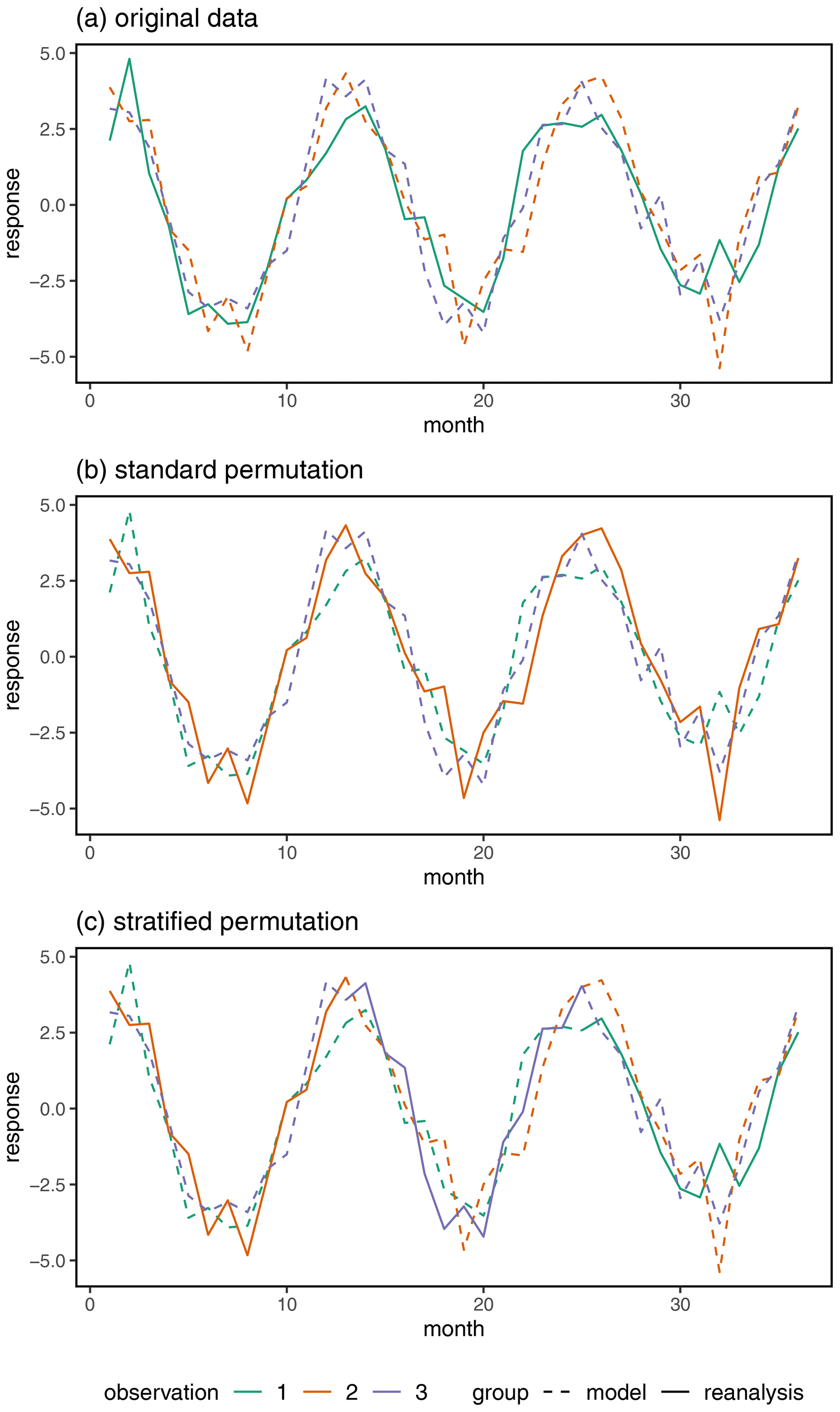
Figure 2 A comparison of the standard and stratified permutation for functional data with the original data.

The stratified permutation test for functional data results in substantially more permutations, correcting the power problem resulting from having a small number of available permutations. Its validity depends on the assumption that $X_j^{\mathrm{M}}\stackrel{\text{i.i.d.}}{\sim }{F}^{\mathrm{M}}$. The independence of the fields $X^{M_j}$ and $X^{{\mathrm{M}}_{j^{\prime }}}$ for $j\ne j^{\prime }$ means that any functional computed from $X^{M_j}$ is independent of any functional computed from $X^{{\mathrm{M}}_{j^{\prime }}}$. An analogous statement is true for the equality of the distributions of these fields. The i.i.d. assumption cannot, thus, be fully verified. However, it is possible to provide some evidence to support it. One can proceed as follows. Choose at random K=100 locations, and for each year n compute

$$G_{j,n}={\displaystyle \frac{\mathrm{1}}{K}}\sum _{k=\mathrm{1}}^K{\displaystyle \frac{\mathrm{1}}{\mathrm{12}}}\sum _{i=\mathrm{1}}^{\mathrm{12}}{X}_n^{M_j}({\mathit{s}}_k,t_i),j=\mathrm{1},\mathrm{2},\mathrm{\dots }\mathrm{15}.$$

That is, we average the temperature values in year n across 100 randomly selected spatial locations for all 12 months in year n. The function G_j,n is an example of a relevant functional of the field $X^{M_j}$ of our infinitely many possible functionals. After computing cross-correlations and applying the Cramér–von Mises test of the equality in the distribution, we found strong support for the assumption of independence and a somewhat weaker, but still convincing, piece of evidence for the equality of distributions.

4 Simulation study

We created a simulation study to better understand the properties of the proposed stratified permutation test compared to a standard permutation test. We set up the study with two goals in mind. First, we wanted to confirm that the proposed method controls the type I error rate for individual tests. This is a minimum requirement for almost any statistical test, so we verify it for the proposed procedures. Second, we wanted to investigate power-related properties of the two tests after adjusting for multiple comparisons. In practice, our testing procedure will be used to perform an inference for a large number of spatial locations. If we only control the type I error rate for individual tests, then definitive statistical conclusions cannot be drawn from the results of many tests since we are unable to quantify the number of errors to expect. Thus, we must use an appropriate multiple comparisons procedure to draw definitive conclusions from our tests. We will make the appropriate adjustments to the multiple comparisons procedure and then compare the power of the two testing procedures.

4.1 Simulation setup

We desired to create simulation data that approximated the kind of data we will be investigating later in this paper. As a first step, we determined the mean and standard deviation of each spatial location for each month across the years 1950–2004 (660 time steps) for the MBCn bias-corrected gridMET data. We then focused on a 32×42 subgrid in the study area for the 300 months between January 1980 and December 2004. Figure 3 displays a heat map of the average temperature of the gridMET data in January 1980 for the 32×42 subgrid. We represent each spatial location by a grid cell for plotting purposes.

We considered three main simulation scenarios. For each distinct simulation scenario, we generated 100 different replications of the scenario. Each replication utilizes 10 data realizations: 9 playing the role of climate model output and the last 1 playing the role of reanalysis data. In the first scenario, all 10 data realizations came from the same data-generating “null” distribution. In the second scenario, the mean of the reanalysis data was shifted by some amount each month for all time steps (described in more detail below). In the third scenario, the mean of the reanalysis data was shifted by some amount each month, starting two-thirds of the way through the time steps (described in more detail below) for a subset of the spatial locations.

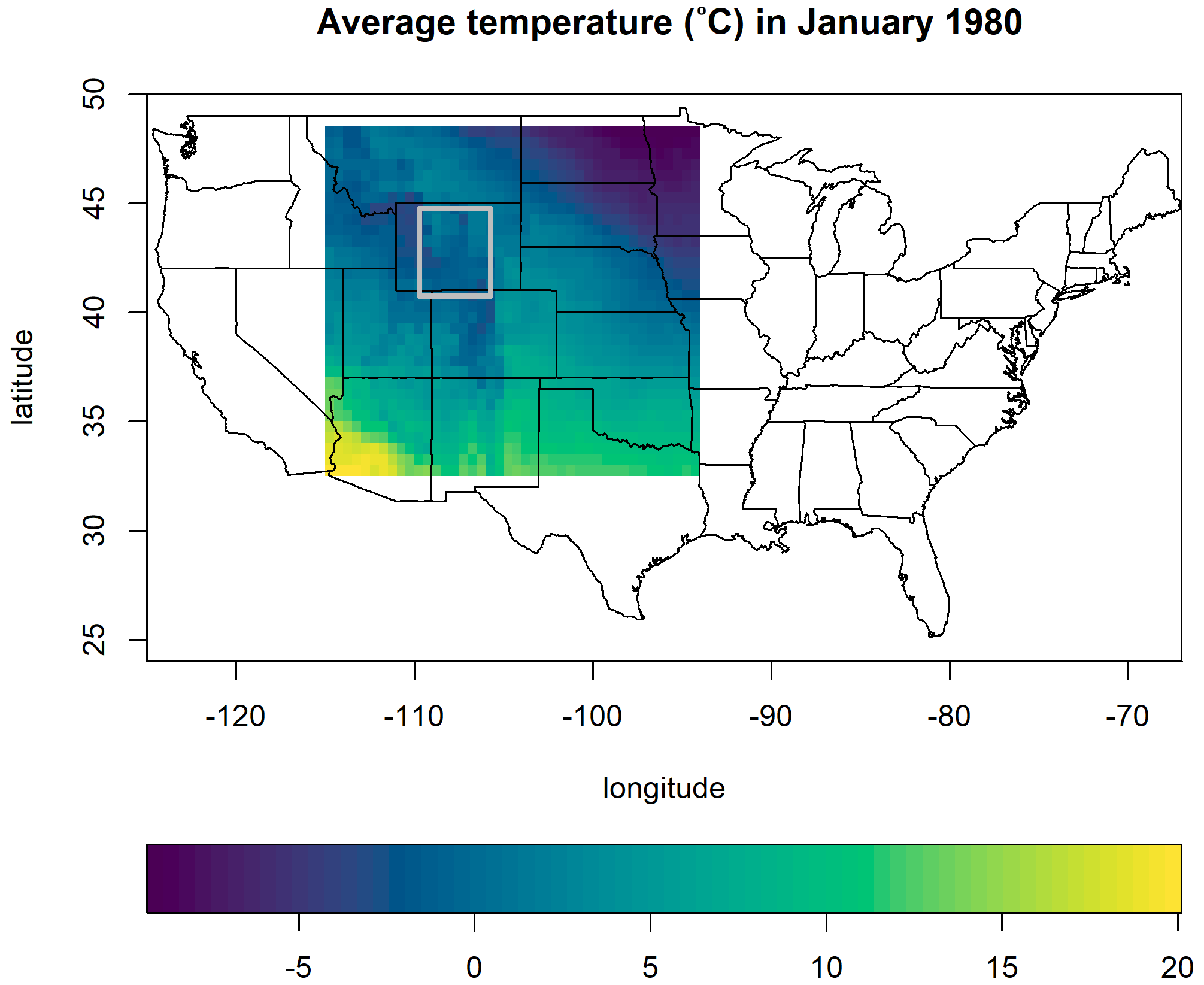
Figure 3 A map providing information about the domain of the simulated data. The colors of the rectangular heat map indicate the average temperature (°C) in January 1980 for the gridMET data. The domain of the heat map also indicates the domain over which data were simulated. The grey rectangle indicates a subarea whose mean changes only for years 21–30 of the simulation study. See the text in Sect. 4.1 for a detailed explanation of the simulation structure.

For each null data set, we simulated AR(1) (autoregressive model of order 1) temporal processes at each spatial location with correlation parameter ρ=0.1 and means and standard deviations equal to the corresponding time step of the gridMET data. To induce spatial correlation at each time step, each simulated response was averaged with the response of the four neighbors that its grid cell shared a border with. To avoid edge effects, we then restricted our analysis to the 30×40 interior grid of the 32×42 subgrid for a total of 1200 spatial locations.

We generated two types of non-null data sets. We generated them using the same basic process as the null data except that the monthly mean temperatures of the reanalysis data sets differ from the monthly mean temperatures for the climate model output data sets. The means differ for the reanalysis data sets in one of the following ways compared to the climate model output data sets: (i) the mean for each month is $m_t+c\times {\text{SD}}_t$, where m_t and SD_t are the temperature mean and standard deviation for that month, respectively, computed from the gridMET data, and where c is a scaling constant, or (ii) starting in January of the 21st year and in each subsequent month, the mean for each month is $m_t+c\times {\text{SD}}_t$ in a contiguous subsection of the study area. We depict this subsection in Fig. 3. In this way, we are able to assess the performance of the procedures when there is a change in the data structure for only a part of the time period considered and for all of the time period considered. Non-null data sets were generated with scaling constants $c=\mathrm{0.15},\mathrm{0.20},\mathrm{0.25},\mathrm{0.30}$, and 0.35 for the first non-null scenario and $c=\mathrm{1},\mathrm{1.25},\mathrm{1.5}$, and 2 for the second non-null scenario.

Two types of tests were performed using each permutation procedure: (i) a test of distributional equality at each spatial location using the distributional equality statistic defined in Eq. (3) and (ii) a test of the difference in mean temperature between the reanalysis and climate model data at each spatial location. More specifically, let

$$\widehat{\mathit{\theta }}\left(\mathit{s}\right)={\displaystyle \frac{\mathrm{1}}{\mathrm{30}\times \mathrm{12}}}\sum _{n=\mathrm{1}}^{\mathrm{30}}\sum _{t=\mathrm{1}}^{\mathrm{12}}{X}_n(\mathit{s},t)$$

denote the 30-year average temperature for a particular set of functions. We tested whether there is a difference in the mean temperature between the reanalysis and climate model data using the following statistic:

$$\widehat{T}\left(\mathit{s}\right)={\displaystyle \frac{\mathrm{1}}{\mathrm{10}}}\sum _{j=\mathrm{1}}^{\mathrm{10}}\left|{\widehat{\mathit{\theta }}}^{M_j}\right(\mathbf{s})-{\widehat{\mathit{\theta }}}^{\mathrm{R}}(\mathbf{s}\left)\right|,$$

where M_j and R denote the functions for a specific climate model and the reanalysis data, respectively. The smallest possible p value for the standard permutation test was 0.10 since there are only 10 possible permutations of the data. Conversely, the smallest possible p value for the stratified permutation test was 0.001 since those tests were implemented with B=999 permutations.

4.2 Simulation results

We begin by verifying that the standard and proposed stratified permutation tests satisfy the minimum standard of controlling for the type I error rate at individual locations. We compute the empirical type I error rate at individual locations using the 100 simulated null data sets described in Sect. 4.1. To reduce the dependence between tests for a particular data set, we randomly selected 20 spatial locations from each replication and then computed the empirical type I error rates for the associated tests across the $\mathrm{100}\times \mathrm{20}=\mathrm{200}$ tests for various significance levels. Since the tests are applied to the null data, a false positive occurs anytime the p value for a test is less than the nominal significance level. Figure 4 displays the empirical type I error rates associated with each significance level for the standard and stratified permutation tests. Different colored symbols are used to distinguish the results for each permutation procedure. The vertical black lines indicate the 95 % tolerance intervals for the empirical type I error rates associated with each significance level. The standard permutation tests can only have associated p values of $\mathrm{0.1},\mathrm{0.2},\mathrm{\dots },\mathrm{1}$. The empirical type I error rates are close to the associated significance level, as expected. One of the 10 empirical type I error rates for the standard permutation tests is outside the tolerance intervals. Zero of the 20 empirical type I error rates are outside the tolerance envelopes for the stratified permutation tests.

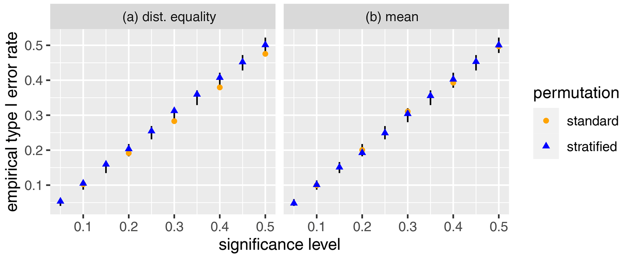
Figure 4 Scatterplots of the empirical type I error rate versus the associated significance level for the two permutation tests. The vertical black lines indicate the 95 % tolerance intervals for the empirical type I error rates associated with each significance level. Panel (a) displays the results for the test of distributional equality between the reanalysis and climate model data, while panel (b) displays the test of mean equality for the reanalysis and climate model data.

Next, we evaluated the power of the standard and proposed stratified permutation tests after adjusting for multiple comparisons. The previous results were only meant to confirm that the testing procedures we utilized satisfied a minimum acceptable standard for a statistical test. When performing many statistical tests, such as in the present context, it is imperative that an appropriate adjustment is made to control a relevant error rate for the many tests, such as the familywise error rate (FWER) or the false discovery rate (FDR). Controlling the FWER in the context of many tests often leads to undesirably low statistical power. Conversely, statistical power is greater when the FDR is controlled instead. Benjamini and Hochberg (1995) proposed a simple procedure for controlling the FDR in the context of multiple comparisons. Benjamini and Yekutieli (2001) proposed a simple procedure for controlling the FDR when test statistics are correlated in a multiple testing context, which we call the BY procedure. Because there was at least some spatial dependence in the tests we performed, we adjusted the p values for our tests using the BY procedure before determining significance. For a specific non-null scenario with a fixed level of c, we computed the empirical power for a specified significance level by determining the proportion of spatial locations across the 100 replicated data sets that had an adjusted p value less than the significance level.

We first summarize the power results for the first non-null scenario, in which there is a difference in the mean temperature of the reanalysis and climate model data for all spatial locations and times. We computed results for both the standard and stratified permutation tests. Figure 5 displays the power results for this scenario when the procedure proposed by Benjamini and Yekutieli (2001) is used to adjust for multiple comparisons. The empirical power of the standard permutation test was zero for all levels of significance, so we do not show the results. When c=0.15 for the stratified permutation test, the power is low to begin with but starts to increase with the significance level. As c increases to 0.35, the power of the stratified tests increases to 1 for all levels of significance. Conversely, because its p values were bounded below by 0.1, the standard permutation test was never able to identify a single location where the distribution of the reanalysis and climate model data differed, regardless of how large the difference was.

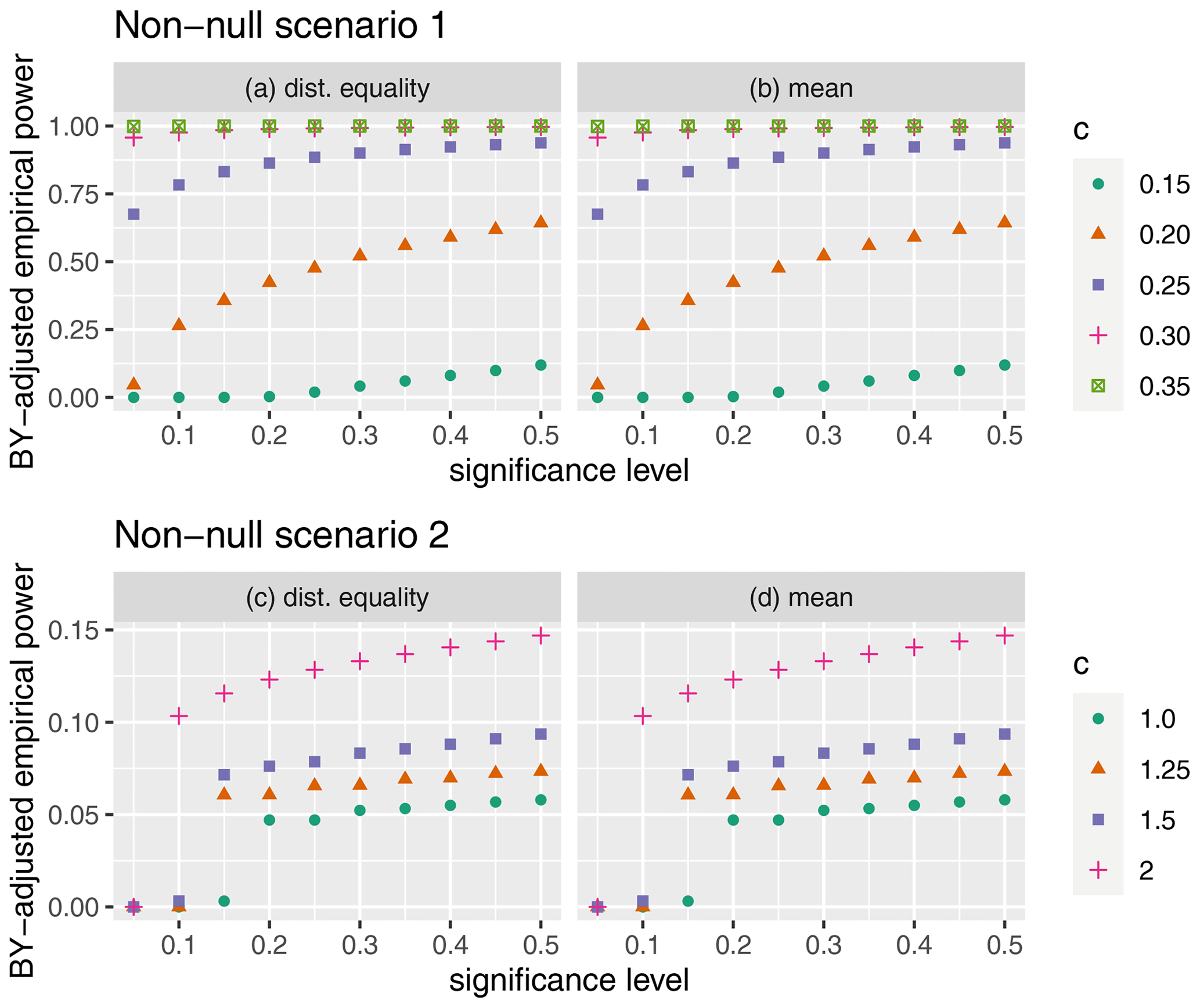
Figure 5 Scatterplots of the empirical power of each permutation procedure versus the associated significance level after using the FDR-controlling procedure proposed by Benjamini and Yekutieli (2001) for the two non-null scenarios. The top panels display the results for non-null scenario 1: panel (a) displays the results for the test of distributional equality, while panel (b) displays the results for the test of mean equality for non-null scenario 1. The bottom panels display the results for non-null scenario 2: panel (c) displays the results for the test of distributional equality, while panel (d) displays the results for the test of mean equality. Note that c indicates the proportional increase in the mean of the reanalysis data.

Next, we summarize the results of the second non-null scenario, in which the mean is shifted for only 121 of the locations for the last 10 years of available data. Figure 5 displays the empirical power when the BY procedure is used to adjust for multiple comparisons. Because the difference in the average temperature was only present for the last 10 years of time, it was more difficult to identify a significant distributional difference at the non-null locations. When c=1, the stratified procedure struggled to detect any differences at usual significance levels, but it was still able to identify some differences for larger significance levels. As c increased to 1.25, 1.5, and 2, the empirical power of the stratified permutation test continued to improve. The empirical power for the standard permutation test was zero for all c and significance levels for this non-null scenario, so its results are not shown in Fig. 5.

In our simulation study, the stratified permutation test exhibits satisfactory power when adjustment is made for the multiple comparisons through the BY procedure. We conclude that if we want adequate power to discover distributional differences between the reanalysis and climate model data sets, the standard permutation test is inadequate. The application of the proposed stratified functional permutation test is required.

5 Climate model evaluation results

We now compare different distributional aspects of the 15 climate model data sets produced by the NA-CORDEX program and the ERA5 reanalysis data, both of which are discussed in more detail in Sect. 2. We perform separate comparisons for each bias-corrected data set (gridMET and Daymet).

We first examine distributional equality for the reanalysis and climate model data. We initially test global distributional equality between F^R and F^M using the test statistic in Eq. (4). For both bias-corrected data sets, the standard permutation tests both return a p value of 0.0625, the lowest possible value for the 16 effective permutations. The stratified permutation test, using a random sample of 999 stratified permutations, returns a p value of 0.001. Next, we consider the spatial test of distributional equality using the test statistic in Eq. (3). We emphasize that we adjust for the multiple comparisons problem using the BY procedure. Figure 6 displays heat maps of the p values less than 0.10 since that is widely used as the largest acceptable level of significance for a hypothesis test. We do not color locations where the p value is more than 0.10. We follow this same pattern in other graphics for this section. For both bias-corrected data sets, substantial portions of the domain exhibit evidence that the distributions of the reanalysis and climate model data are not in agreement.

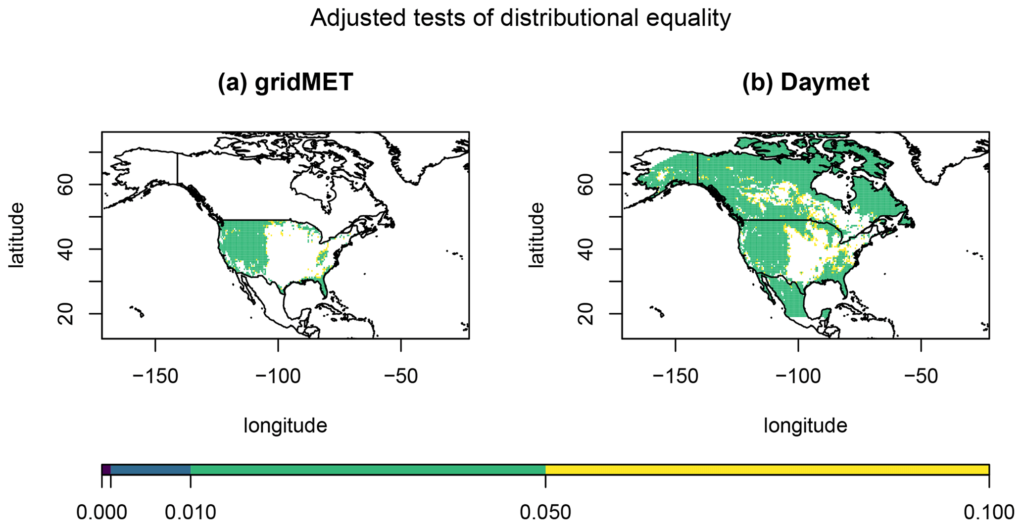
Figure 6 Heat maps of the BY-adjusted p values ≤0.10 for the distributional equality test based on the statistic in Eq. (3) for (a) the gridMET bias-corrected data and (b) the Daymet bias-corrected data.

Next, we identify ways in which the distributions differ. We test the hypotheses in Eq. (5) regarding θ^R(s)=θ^M(s) for several characteristics: the 55-year mean temperature, median temperature, temperature standard deviation, and temperature interquartile range.

As mentioned in Sect. 3.4.1, we need to determine a suitable test statistic for testing these hypotheses. In our context, we wish to assess discrepancies in the 55-year behavior of the climate model characteristics in comparison to the reanalysis characteristics. Thus, it seems sensible to begin by summarizing the characteristics of the 55-year functional time series. Specifically, for the partial realization of X(s), we compute a statistic that summarizes some characteristic of the distribution over the 55 years. For example, the mean behavior would be summarized by

$$\widehat{\mathit{\theta }}\left(\mathit{s}\right)={\displaystyle \frac{\mathrm{1}}{\mathrm{55}\times \mathrm{12}}}\sum _{n=\mathrm{1}}^{\mathrm{55}}\sum _{t=\mathrm{1}}^{\mathrm{12}}{X}_n(\mathit{s},t),$$

which we use to summarize the average temperature over the specified time frame. Similarly, since there are $\mathrm{55}\times \mathrm{12}=\mathrm{660}$ observed values in each time series, the 0.50 quantile statistic would be the empirical 0.50 quantile of the 660 observed data values at location s, i.e., of the set $\mathit{\left\{}{x}_{\mathrm{1}}\right(\mathit{s},\mathrm{1}),x_{\mathrm{1}}(\mathit{s},\mathrm{2}),\mathrm{\dots },x_{\mathrm{1}}(\mathit{s},\mathrm{12}),\mathrm{\dots },x_{\mathrm{55}}(\mathit{s},\mathrm{1}),\mathrm{\dots },x_{\mathrm{55}}(\mathit{s},\mathrm{12}\left)\mathit{\right\}}$. In order to quantify the discrepancy of the test statistics across the reanalysis and climate model data, we use the average absolute difference between statistics across the reanalysis and climate model groups. Formally, we compute the statistic

$$\begin{array}{}\text{(6)}& \widehat{T}\left(\mathit{s}\right)={\displaystyle \frac{\mathrm{1}}{N_M}}\sum _{j=\mathrm{1}}^{N_M}\left|{\widehat{\mathit{\theta }}}^{\mathrm{R}}\right(\mathit{s})-{\widehat{\mathit{\theta }}}^{M_j}(\mathit{s}\left)\right|\end{array}$$

for each spatial location and assess the significance using standard and stratified permutation tests. For all tests below, we evaluate the significance of the test at each spatial location after using the BY procedure to control the FDR. In the following discussion, we will typically drop the “55-year” qualifier for parameters and statistics for brevity.

We first examine the results related to measures of center. We test equality of the mean temperature of the reanalysis and climate model data at each spatial location, and similarly, we test equality of the median temperature. Figure 7 displays heat maps of the BY-adjusted p values ≤0.10 for these tests. The temperature means for the reanalysis and climate model data tend to differ in the western part of the United States and along the eastern coastline of the United States. We also see evidence of mean temperature differences in much of Canada and Mexico for the Daymet data. There are fewer locations exhibiting a difference in median temperature along the eastern coastline of the United States compared to a difference in mean temperature, though the opposite pattern is observed in the middle part of the United States. For the Daymet data, the locations exhibiting a mean or median temperature difference in Mexico tend to be similar, though there are fewer locations in Canada exhibiting a difference in median temperature.

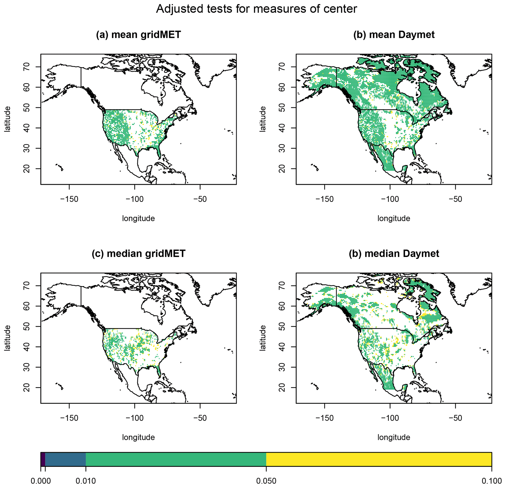
Figure 7 Heat maps of the BY-adjusted p values ≤0.10 when performing the test of equality of (a) mean temperature using the gridMET data, (b) mean temperature using the Daymet data, (c) median temperature using the gridMET data, and (d) median temperature using the Daymet data.

Next, we consider tests for dispersion-related parameters, specifically the standard deviation and interquartile range (IQR) of the data. We test equality of the temperature standard deviation for the reanalysis and climate model data at each spatial location, and similarly, we test equality of the temperature interquartile range. Figure 8 displays heat maps of the BY-adjusted p values for the locations where the p value ≤0.10 for these tests. Overall, we see similar patterns for a fixed characteristic (standard deviation or interquartile range) across both bias-corrected data sets. Similarly, if we fix the data set (gridMET or Daymet), we see similar p-value patterns across the measure of spread. However, there are noticeably fewer locations with adjusted p values ≤0.10 for the tests of equality of the temperature interquartile range compared to tests for standard deviation.

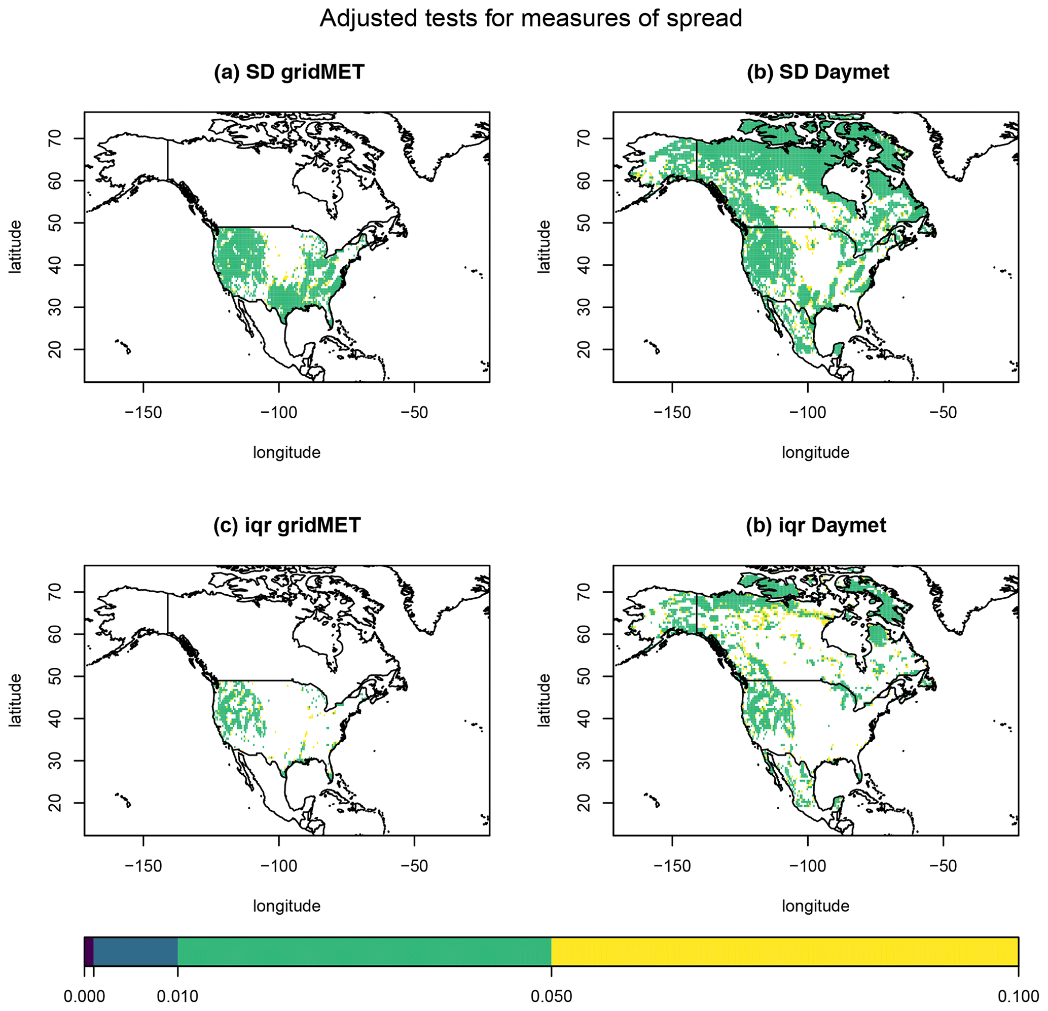
Figure 8 Heat maps of the BY-adjusted p values ≤0.10 when performing the test of equality of (a) temperature standard deviation using the gridMET data, (b) temperature standard deviation using the Daymet data, (c) temperature interquartile range using the gridMET data, and (d) temperature interquartile range using the Daymet data.

Lastly, we focus on the results of tests related to characterizing the functional nature of the data. We want to formally compare the functional behavior of the reanalysis and climate data over time at each spatial location. Consequently, we fit a B-spline with 276 equidistant knot locations over the 660 months of temperature data available at each spatial location (essentially five knots per year), resulting in 276 estimated coefficients for each spatial location. We then compared whether the coefficients associated with the reanalysis data were equal to the coefficients for the climate model data. Such a test allows us to determine the times when the climate model data patterns disagree with the reanalysis data. For each spatial location, we computed the statistic

$$\begin{array}{}\text{(7)}& \widehat{T}\left(\mathit{s}\right)={\displaystyle \frac{\mathrm{1}}{\mathrm{276}{N}_M}}\sum _{j=\mathrm{1}}^{N_M}\sum _{k=\mathrm{1}}^{\mathrm{276}}\left|{\widehat{\mathit{\theta }}}_k^{\mathrm{R}}\right(\mathit{s})-{\widehat{\mathit{\theta }}}_k^{M_j}(\mathit{s}\left)\right|,\end{array}$$

where ${\widehat{\mathit{\theta }}}_k^{\mathrm{R}}\left(\mathit{s}\right)$ is the kth estimated coefficient for the reanalysis data at location s, and ${\widehat{\mathit{\theta }}}_k^{M_j}\left(\mathit{s}\right)$ is the kth estimated coefficient for the jth climate model data set at location s. Figure 9 displays heat maps of the p values for the locations where the test is significant at α=0.10. Perhaps unsurprisingly, the results for this test are similar to those for the test of distributional equality. We see significant differences in the coefficients for the reanalysis and climate model data in the western part of the United States, as well as the northern parts of Canada and the central parts of Mexico.

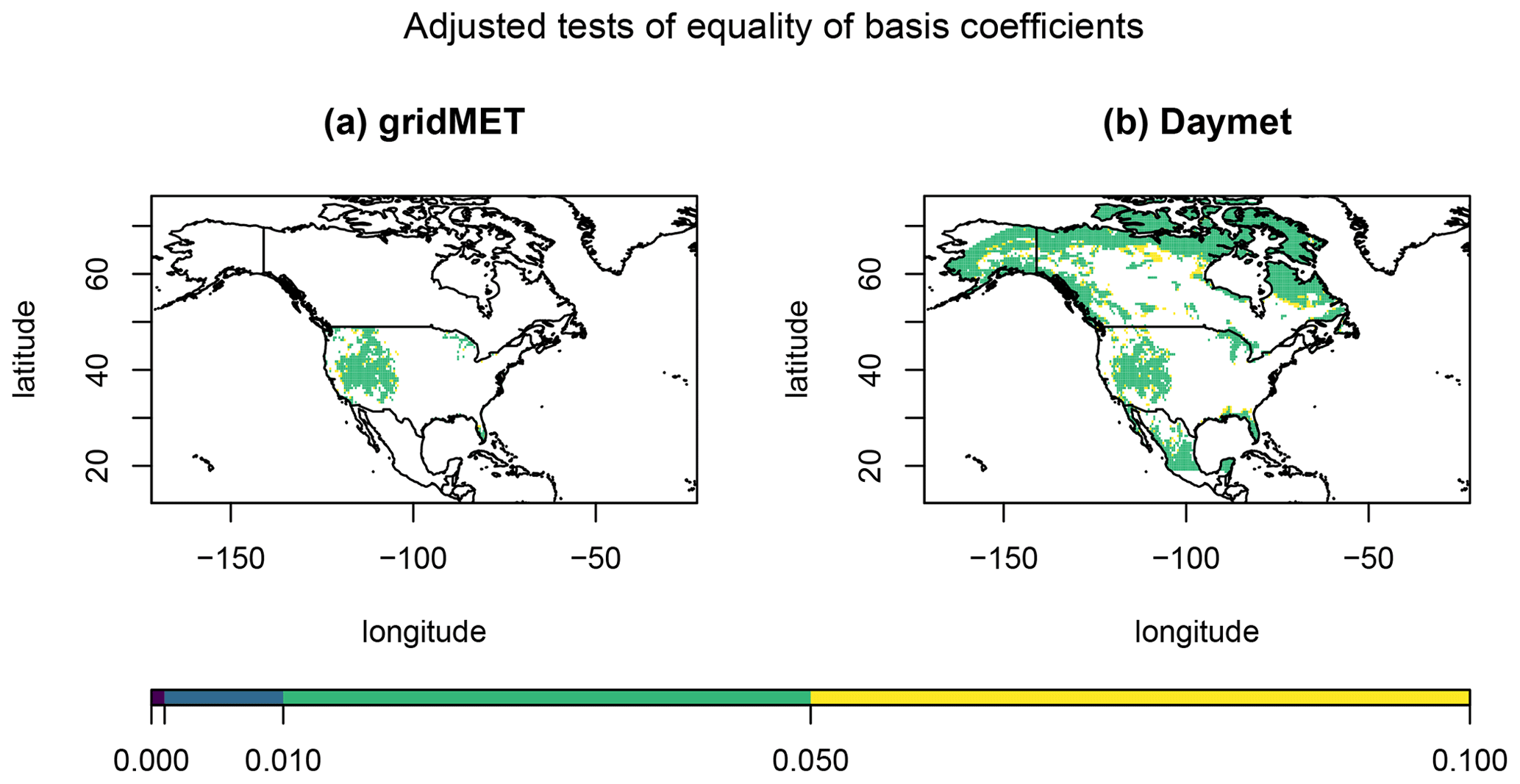
Figure 9 Heat maps of the BY-adjusted p values ≤0.10 for (a) the gridMET bias-corrected data for a test of coefficient equality and for (b) the Daymet bias-corrected data for a test of coefficient equality.

Comparison of our results with previous results is difficult as the studies we are familiar with focus on evaluating specific distributional characteristics of climate models compared to observational data in specific places. Additionally, the reference data sets may differ, making it difficult to compare analyses. Lee et al. (2019) provide the most similar comparison to our present analysis, in which they compare temperature trends between reference and climate model data over seven regions in the continental United States. This comparison was made for summer and winter seasons for three time periods: 1895–1939, 1940–1979, and 1980–2005. Lee et al. (2019) aggregate their results over seven large regions, whereas we make an inference at a finer spatial scale. The time periods of our comparison also differ. Additionally, Lee et al. (2019) separate summer and winter behavior so that they can look at trends, whereas we consider behavior over the entire year. A key difference in our comparisons is that we use the ERA5 data as our reference data set, while Lee et al. (2019) use the Global Historical Climatology Network – Daily (GHCN-Daily) data set (Menne et al., 2012). Those caveats aside, our analysis tends to find the most agreement between the temperature distributions of the reference data and the climate model data in the middle part of the United States with less similarity in the eastern and western parts. The analysis by Lee et al. (2019) tended to find more similar temperature trends in the eastern and western parts of the United States and less similarity in the middle part of the United States (see Fig. 7 of Lee et al., 2019). However, little can be concluded from this disagreement, because our analyses differ in approach, reference data set, and temperature characteristic; their similarity is limited to the variable of interest (temperature) and location (continental United States).

6 Discussion

We have presented a new stratified permutation test appropriate for comparing the distributional characteristics of climate model and reanalysis data. In our context, a standard permutation test, even when adjusted to preserve spatial and temporal dependence, is not effective for performing comparisons because there are few unique permutations, limiting the discriminating power of the test. The proposed permutation procedure allows for the creation of millions of unique permutations, which substantially improves the power of the testing procedure for usual significance levels. Additionally, the new testing procedure makes it possible to apply proven approaches for addressing the multiple comparisons problem, which are ineffective in the context of standard permutation tests.

We applied our stratified permutation test in comparing the distributional characteristics of bias-corrected NA-CORDEX climate model data output to the ERA5 reanalysis data for monthly temperature data over the years 1950–2004. We used the testing procedure proposed by Benjamini and Yekutieli (2001) to control the FDR of our tests. The temperature distributions of the NA-CORDEX and ERA5 data sets tended to be most similar in the middle and eastern parts of the United States, with distributions tending to significantly differ in parts of Canada and most of Mexico. Our analysis focused mostly on simple characteristics of the data like the 55-year mean, median, standard deviation, and interquartile range of the temperatures. We also considered a broader test of distributional equality and a comparison of the coefficients of a functional representation of the temperature time series. However, these tests could be done for more refined characteristics of the data such as looking at features for particular seasons (average temperature in a particular month), looking at distributional changes over particular time periods (the decadal changes in the interquartile range of temperature) or looking at smaller-scale characteristics (rate of change characteristics for hourly level data). A possible critique of our analysis is that the NA-CORDEX climate model data sets may not be independent. Specifically, several of the data sets use conditions from the same GCM, so one could argue that the data for RCM–GCM combinations sharing the same GCMs are not independent. To assess the impact of this, we ran a secondary analysis using only the NA-CORDEX climate model output for models using different GCMs. The results for the secondary analysis, shown in the Supplement, are very similar to the results discussed in Sect. 5. Another reasonable critique might be that different GCMs do not follow the same probability distribution. However, without this assumption, no replications could be considered, and statistical inference would be practically infeasible. Based on the similarity of the power results for tests of distributional equality and mean equality in Sect. 4.2, one may wonder whether one test is preferred over the other. The choice only depends on the goals of the researcher. A test of distributional equality can only inform the researcher of whether the overall distribution of the reanalysis data is similar to the climate model output; rejecting the null hypothesis does not tell the researcher how the distributions differ. Do they differ with respect to center, spread, quantile behavior, and so on? Conversely, a test based on specific distributional attributes like the mean, median, or interquartile range only evaluates whether the distributions differ with respect to a single characteristic. Failing to reject the null hypothesis does not mean that the distributions being compared do not differ; it only means they do not differ significantly with respect to that single characteristic. Ultimately, the tests provide complementary information, and the researcher must choose the information that is most important for their study.

Angélil et al. (2016) recommend using multiple reanalysis data sets when performing climate model evaluation, so one could augment the presented analysis by including reanalysis data from NASA's MERRA2 (Modern-Era Retrospective analysis for Research and Applications, Version 2) program and the Japanese 55-year Reanalysis (JRA-55; Kobayashi et al., 2015). Those data sets have different spatial domains and time periods over which the data are available, so adjustments would have to be made to account for these differences. However, we hope to provide a more thorough analysis involving these additional reanalysis data sets to investigate the similarity of behavior between the reanalysis data and the climate model output data. Additionally, our present investigation focused only on temperature, which tends to behave well in the sense of having a relatively symmetric, bell-shaped distribution when considering observations at a similar time and place. Another variable of great scientific interest is precipitation, which behaves very differently from temperature. Precipitation data can be highly skewed and zero-inflated, which can require additional analysis considerations that are beyond the scope of this paper, even when minimal distributional assumptions are made with respect to the proposed test. Additionally, Dee et al. (2016) warn that “Diagnostic variables relating to the hydrological cycle, such as precipitation and evaporation, should be used with extreme caution”. However, we hope to investigate the behavior of precipitation for reanalysis and climate model output data in future efforts.

Some readers may be interested in comparing the spatial patterns of p values for the BY-adjusted p values of the stratified permutation test with the unadjusted and BY-adjusted p values of the standard permutation test as well as the unadjusted p values of the stratified permutation test. The standard permutation procedure has much lower testing power than the stratified permutation test. While one can have significant results at many locations when using the standard p values, the BY-adjusted p values will have zero significant locations. One implementation of the Benjamini–Yekutieli (BY) procedure takes the standard p values and adjusts them upward so that testing can be performed at a fixed significance level while addressing the multiple comparisons problem. Since the BY-adjusted p values are uniformly larger than the unadjusted p values, any location significant after the BY p-value adjustment is automatically significant at the same significance level for the unadjusted p values. However, we would also expect additional significant locations when using the unadjusted p values; the locations significant for the unadjusted p values will extend from the locations that are significant for the adjusted p values. Figure S5 in the Supplement provides a visual comparison of this behavior for a test of distributional equality based on the statistic in Eq. (3).

Our stratified permutation test is highly scalable since tests can be parallelized across permutations or spatial locations. In the analyses we considered, the time needed to perform the tests increased linearly with the number of spatial locations and time steps. We analyzed monthly rather than daily data in order to reduce the run time and because our focus was on decadal climate patterns. However, especially for shorter time periods, there could be distributional characteristics that can only be studied through the examination of daily or even hourly data. If the data sets cannot be held in memory at one time, then the stratified permutation test can still be applied by summarizing statistics one location at a time, assuming that the spatiotemporal data are structured so that the responses for specific spatial locations at specific time steps for a specific model can be accessed conveniently. This modified implementation of the test would likely be slower than when the data can be held in memory, but this would allow for the analysis of much larger data sets. Alternatively, one could first represent the data in a functional form prior to analysis, e.g., using the spatiotemporal sandwich smoother of French and Kokoszka (2021), which would dramatically reduce the memory space needed to represent the data structure or smoothed values. Tests could then be performed using the smoothed data, the functional parameters, or the related characteristics. We hope that the methodology we developed and the insights we presented will stimulate related research on comparing model and historical climate data using the increasingly available data products.