Forecasting springtime rainfall in southeastern Australia using empirical orthogonal functions and neural networks

Forecasting rainfall into the next season remains highly challenging and is normally presented in terms of probabilities rather than the expected rainfall as measured by rain gauges. I show here that, in favourable cases, for the selected times of the year and selected geographical regions, it is possible to obtain useful quantitative forecasts of rainfall with a series of relatively simple steps. One such instance explored in this work is the prediction of austral springtime rainfall in SE Australia regions predominantly based on the surrounding ocean surface temperatures during the winter.

In the first stage, I search for predictors by exploring correlations between the target rainfall and ocean surface temperatures at earlier times. In addition to standard ocean climate indicators such as El Niño or the Indian Ocean Dipole, other typical patterns of variation are captured in terms of the temperatures of selected ocean areas. When characteristic patterns of correlation are discovered, they are included in the predictor selection in the form of expansion in terms of the empirical orthogonal functions (EOFs). EOF expansions can provide very strong signals. For example, in the case of the Indian Ocean, during the winter, the dominant EOF shows a stronger correlation with future rainfall than the commonly used Indian Ocean Dipole.

The technical part of the forecast model is provided by deep learning artificial neural networks, where I use the information sources with the strongest correlation in relation to the historical rainfall data as the inputs. The networks are trained on past rainfall data, and the output is a quantitative forecast based on the current state of the predictors. The resulting hindcasts appear to be accurate for September and October and less reliable for November. I also present model forecasts for rainfall during the 2024 austral spring in the selected SE Australia regions.

1 Introduction

Southeastern Australia, including the Murray–Darling Basin, is a highly productive agricultural region largely dependent on adequate rainfall, which provides the irrigation water needed for high-value crops. Accurate prediction of water availability several months in advance would greatly aid in crop planning and management. The medium-term forecasts for the farming community are regularly published by the Australian Bureau of Meteorology and the state bodies, e.g. Agriculture Victoria.

The most important influence on future rainfall in Australia is the ocean temperature surrounding the continent. For more than 50 years, Indian Ocean sea surface temperatures (SSTs) have been known to affect rainfall over the continent. A comprehensive history of earlier research is available in Ummenhofer et al. (2008). The configuration of the Indian Ocean SST is accepted as one of the major climate drivers over the large regions of the three continents at its boundaries. These SST conditions are codified as the Indian Ocean Dipole (IOD) index, which is defined as the difference between the anomalies on the western side (10° N to 10° S and 50 to 70° E) and those on the eastern side (0 to 10° S and 90 to 110° E) of the basin. During its negative phase, westerly winds at tropical latitudes accumulate warmer surface water north of Australia, leading to increased rainfall over the continent.

The influence of Indian Ocean teleconnections on the rainfall in SE Australia was explored by Cai and Cowan (2008), Ummenhofer et al. (2009), and Cai et al. (2011a), who established another indicator of the SST configuration of the Indian Ocean to the northwest of Australia that has an even stronger influence than the IOD on the rainfall in the southeast of the continent. The meridional temperature gradient – defined in Ummenhofer et al. (2009) as the difference in terms of SST anomalies between the regions sI (centred at 30° S, 95° E) and eI (centred at 10° S, 110° E), both with a 10° surround – correlates strongly with the rainfall during both dry and wet years. Closely linked to Indian Ocean conditions, subtropical ridge position and intensity are also strongly correlated with rainfall in SE Australia (Cai et al., 2011a, b; Timbal and Drosdowsky, 2012).

Pacific Ocean conditions, as reflected in the El Niño–Southern Oscillation (ENSO) phase, influence the weather throughout Australia. The relationship between ENSO and the weather system movements and, ultimately, the rainfall in SE Australia is very variable, with complicated dynamics (Lim et al., 2016; Hauser et al., 2020). While ENSO and the IOD are not independent (Wang et al., 2019), ENSO data contain information that is complementary to that of the IOD and are the second most important input in forecasting rainfall in Australia.

The variations in the ocean conditions surrounding Australia are most prominent during austral winter and spring, when both the IOD and ENSO show greater departures from the neutral state (e.g. Lim et al., 2021). Larger departures from the neutral range create favourable conditions for medium-range forecasting of spring rainfall.

A comprehensive study devoted specifically to oceanic and atmospheric predictors of rainfall and runoff over SE Australia was conducted by Kirono et al. (2010), who explored 12 predictors during all seasons of the year. The study found that the best predictors of rainfall for the springtime period were SST in the Niño-4 area and the depth of the Pacific Ocean thermocline represented as the second empirical orthogonal function (EOF) of the 20 °C isotherm (Ruiz et al., 2006). The use of EOFs as predictors of rainfall was also explored by Drosdowsky and Chambers (2001), who reported a significant correlation between the first two Pacific and Indian Ocean EOFs and the subsequent rainfall.

The present study was designed to produce springtime forecasts during the winter months, which limits the choice of predictors to those where data for the previous months are available within 2 weeks after the end of the month. For this reason, important information contained in the temperature profiles of the interior of the oceans, including the thermocline, is presently not included. This restriction is not present in earlier hindcasting studies where all the predictors are available. In accordance with Kirono et al. (2010), correlations between different Niño SST regions during the winter and the springtime rainfall were evaluated, and, for the most recent 25 years, Niño 3.4 was better correlated with rainfall than Niño 4 was; hence, it was selected as one of the predictors for all winter forecasts.

Over decades, Pacific and Indian Ocean climate patterns slowly change (Han et al., 2014; McKay et al., 2023a). The collected data become less relevant over time. In this work, I found that pre-1950 data seldom contribute useful information, and, for all hindcasting tests, the best results were obtained with the datasets starting in 2000.

In the following section, I extend the earlier search for correlations between different climate drivers and rainfall in the spring. To produce current forecasts, my method uses deep learning artificial neural networks to integrate full historical information from all included climate drivers. With this approach, I integrate many years of past data from many climate drivers to capture typical nonlinear patterns of climate system evolution and, during the winter, produce a springtime forecast. The two sources seldom mentioned in routine periodic forecasting reports, the meridional gradient and the dominant EOFs, greatly improve the outcomes in all hindcast tests. Earlier work on machine learning in integrating information from many climate drivers (Feng et al., 2020) used a very different method (random forest model for aggregating the data).

Understanding of the physical basis of specific climate patterns is not used in this work and in most other works utilising artificial neural networks. The physical processes are the sources of data, and, based on the data, the networks recognise the patterns and provide the answers for the practical task of medium-term rainfall forecasting.

The three rainfall regions explored are, as defined by the Australian Bureau of Meteorology, southeastern Australia, Victoria, and the Murray–Darling Basin. The next section describes the search for the best input data streams, and the subsequent section describes the hindcasting and forecasting of the future rainfall with deep learning nonlinear neural networks. Many of the details, as well as the forecasting outcomes that became available during the revision of the paper, are relegated to the Supplement.

2 Search for climate variables that correlate with future rainfall

The primary search tool is the Pearson correlation coefficient, which is used to measure the linear relationship between the temperatures and rainfall at different locations. Some of the valuable earlier works (e.g. Ummenhofer et al., 2008) explored the correlation between driving variables correlated with rainfall and rainfall at the same time of the year. Here, I am primarily interested in the predictive power of such variables; hence, I search for the correlation between a variable and rainfall in the following season. As an example, the correlation coefficient between the time series of August SST averages and November rainfall in southeastern Australia is shown in Fig. 1.

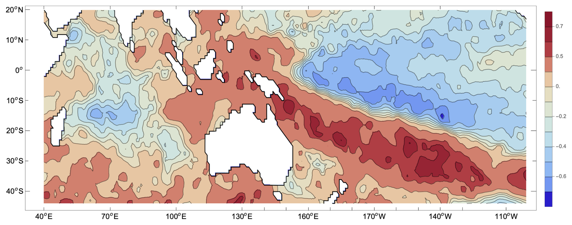
Figure 1 The correlation coefficient between the average SST during August and rainfall in November in southeastern Australia during the period 2000–2023; the dataset used was HadISST4.01. The strong feature seen east of the Australian continent contains information that is useful for the forecasting of November rains. Two more examples of ocean maps are shown in Sect. S4.

A rigorous linear tool that is able to capture significant ocean SST features is the representation of SST fields as an expansion into EOFs. The intent behind my use of EOFs as a forecasting tool is the reduction of the large and partly redundant historical data contained in the SST at each position into smaller sets of independent data ordered by descending importance. EOFs were determined using the method and the software of Dawson (2016). For example, ocean surface temperatures (ERSST data) at each position during the month of July between 1950 and 2024 are used as an input. As the resolution of the data is 2 °, this represents a 41 × 31 matrix for each year. The resulting analysis defines EOFs for the selected area and for the month of July. The SST distribution for July of each year is represented as a linear sum of EOFs, where coefficients in the sum change every year. The time series of the coefficients contains SST history information in a condensed form without redundancy, which leads to a simpler and more accurate analysis. The EOFs for the two studied temporal periods, 1950–2024 and 2000–2024, are very similar, and I choose a longer period, which results in slightly better accuracy in applications.

The dominant July EOF for the Indian Ocean, shown in Fig. 2, is spatially similar to the definition of the IOD. During July, the time series of its strength (expansion coefficient) correlates with rainfall in the September–October period more strongly than the time series of the IOD. For example, the correlation coefficient between the Murray–Darling Basin rainfall during the September–October period and the dominant Indian Ocean EOF in July is 0.66. In this example, the next best indicator is the meridional gradient, with a correlation coefficient of 0.55, whereas, for the IOD, it is 0.44. The seemingly modest differences are very significant in hindcast testing of predictability.

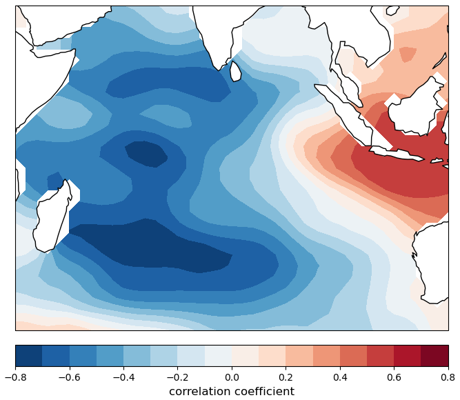
Figure 2 The first EOF for the month of July and for the Indian Ocean region shown in the figure. The expansion in EOFs is calculated from the time series of July SSTs between 1950 and 2024 using ERSSTv5 data. The scale in the figure shows the correlation between the time series of the original SST and the coefficient of the first EOF at each spatial position. High values of the correlation indicate a high degree of covariation between the SST and EOF.

After suitable ocean variables are identified, an easy way to check leading times between the SST signal and the subsequent rainfall is to plot correlations between monthly averages of the variable and the rainfall in each region. In Fig. 3, I illustrate the correlation coefficient between Indian Ocean variables and rainfall in southeastern Australia over all months. A table with all the variables used in prediction is given in Sect. S2.

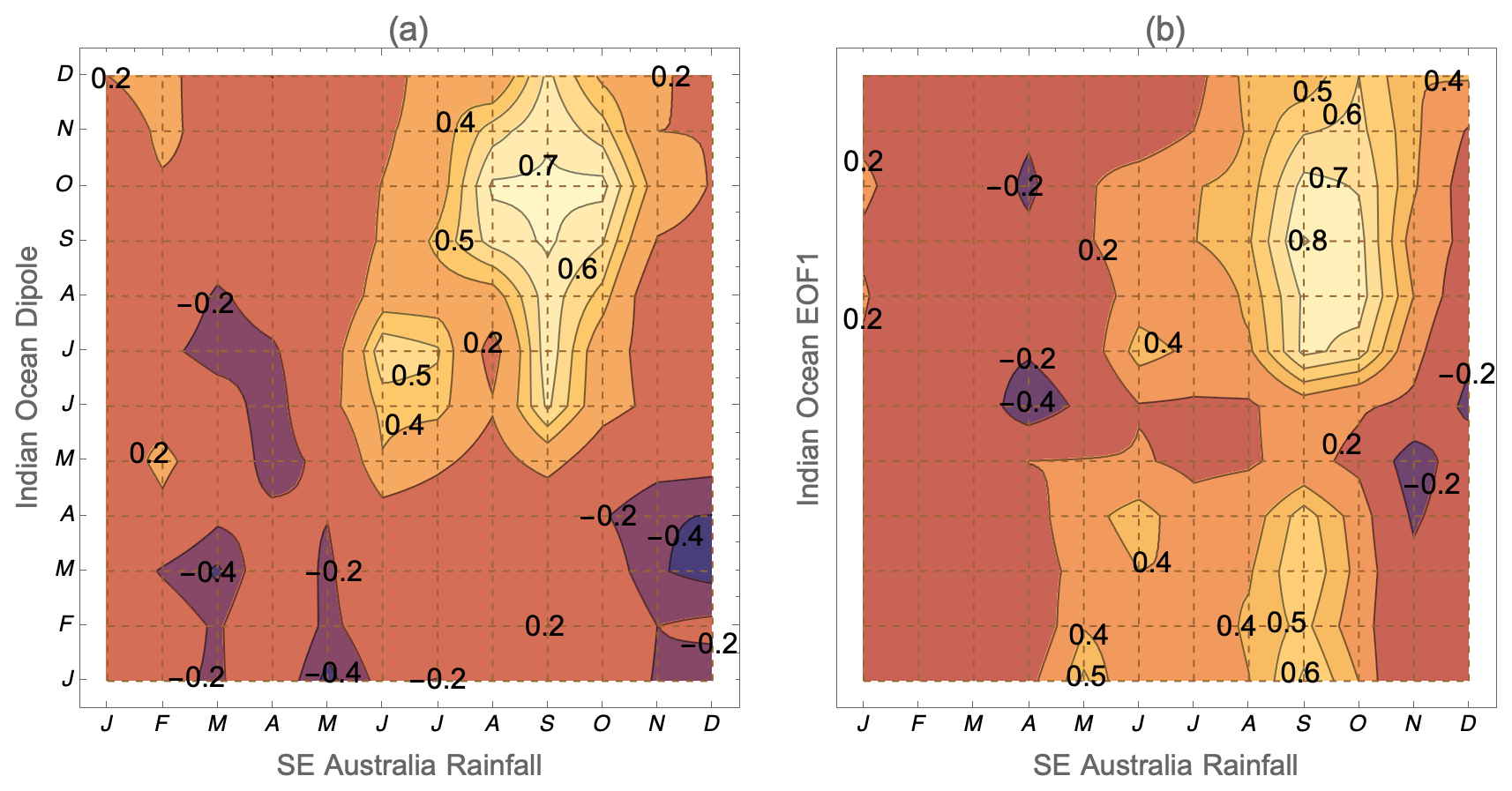
Figure 3 Correlation coefficient between the rainfall in southeastern Australia in any month and the (a) IOD and (b) dominant Indian Ocean EOF during another month. The interesting parts of the diagrams are the months preceding the rainfall, which are in the lower-right section of the images, below the shaded area. The images show that rain is strongly correlated with ocean indicators only in the spring. It is easily visible that, in July, the future September–October rain is more strongly correlated with the EOF than the IOD, whereas the opposite is true in June.

3 Hindcasting and forecasting of springtime rainfall

3.1 Forecasting chaotic dynamics

For a deterministic chaotic system, past data are, in principle, sufficient to reconstruct the underlying dynamics (Takens, 1981). For a multidimensional system with additive noise, this will only be approximately possible, and both linear and nonlinear methods have been extensively tested. Linear methods are less sensitive to errors in the input, and multiple linear regression is often the method of choice (e.g. Maher and Sherwood, 2014; Hudson et al., 2017; Lim et al., 2021; McKay et al., 2023b). With more data, nonlinear methods, usually either delay coordinate embedding or neural networks, perform better (Weigend and Gershenfeld, 1994).

Once the information sources about future rainfall have been identified, there is a choice between a number of possible linear and nonlinear forecasting methods. The task is difficult as regional climate changes over decades (Han et al., 2014) make older data misleading, and the useful history period is short (see discussion in Sect. S3). I find that the best results in hindcasting are obtained using only the records obtained since the year 2000. An example showing the results when longer periods are used is shown in Sect. S3. Based on the performance, data from 1950 were used in calculations of EOFs but not elsewhere.

For the period since 2000, there are not enough data to find similar past states, and delay coordinate embedding is not accurate. In my tests with springtime rainfall, deep learning artificial neural networks performed better than linear methods or delay coordinate embedding (Sect. S7). Neural networks have been used in climate research on many occasions, e.g. El Niño or IOD forecasting (Nooteboom et al., 2018; Ham et al., 2019; Ratnam et al., 2020). More recently, very-large-scale artificial intelligence models have been developed for weather forecasting over a 10 d period (e.g. Lam et al., 2023; Bi et al., 2023), but they also have intrinsic limitations in terms of accuracy (Seltz and Craig, 2023).

3.2 Training of neural networks

The choice of predictors and settings in the training process is strictly empirical. The guiding principle in the selection is a decrease in the root mean square error (RMSE) of the differences between the data and the hindcasts in the validation segment. As is common with neural network training, the procedure is largely a matter of trial, error, and gradual improvement (Hastie et al., 2009; Yong, 2022). After extensive testing, I selected networks consisting of three to five linear layers and one tanh nonlinearity. A total of 25 years of data were typically divided into 14–17 years for training, 5–7 years for validation, and 1 or more years for hindcasting and/or forecasting.

Many runs were performed for each basin, starting the networks with different random learning rates. The scatter in the results is shown as faint grey lines. During training, network connection strengths are varied until the network settles within the local minima of the cost function (Yong, 2022, Sect. 6.3). Averaging over the results of many runs is accepted as the result. Notably, because of random starts, repeating the runs results in slightly different hindcasts. These differences in the results for rainfall over a 2-month period are typically several millimetres, which is small compared with the intrinsic errors of the process.

Low learning rates lead to a slow drift towards one of the minima in the error landscape, whereas high learning rates allow the system to probe many of the neighbouring minima, leading to increased scatter in the results of different runs but often higher accuracy when the mean value is used. The input time series should be scaled to have the same or almost the same norm as relative magnitudes affect the nonlinear process of training.

Network training is performed using the elaborate and comprehensive neural network software developed by Wolfram Research and which forms a part of Mathematica. During neural network training, the available short sequence of target rainfall data is used to determine many synaptic weights. The networks rapidly drift towards the overfitting regime, i.e. a perfect agreement during the training period but decreasing accuracy in the validation period. The software automatically selects the result that corresponds to the lowest validation errors. To make the best use of the limited data, for the final forecast, the validation segment is extended to the year of the forecasts, and the test segment is omitted.

3.3 Robustness and accuracy of the procedure

The process of predictor choice and network training must pass several tests to confirm the credibility of the results. The networks formed with only the data available a few years before the present should perform similarly to the networks trained using all of the data. When forecasting is robust, variations in the division between the validation and test segments do not change the results substantially. The years when networks are inaccurate in hindcasting signify incomplete input at that time, possibly due to the relatively brief training period.

An example of forecasting with and without a test segment is shown in Fig. 4. Terminating the validation segment in the year 2019 only slightly decreased the fit over the 2020–2023 period and practically left the forecast unchanged.

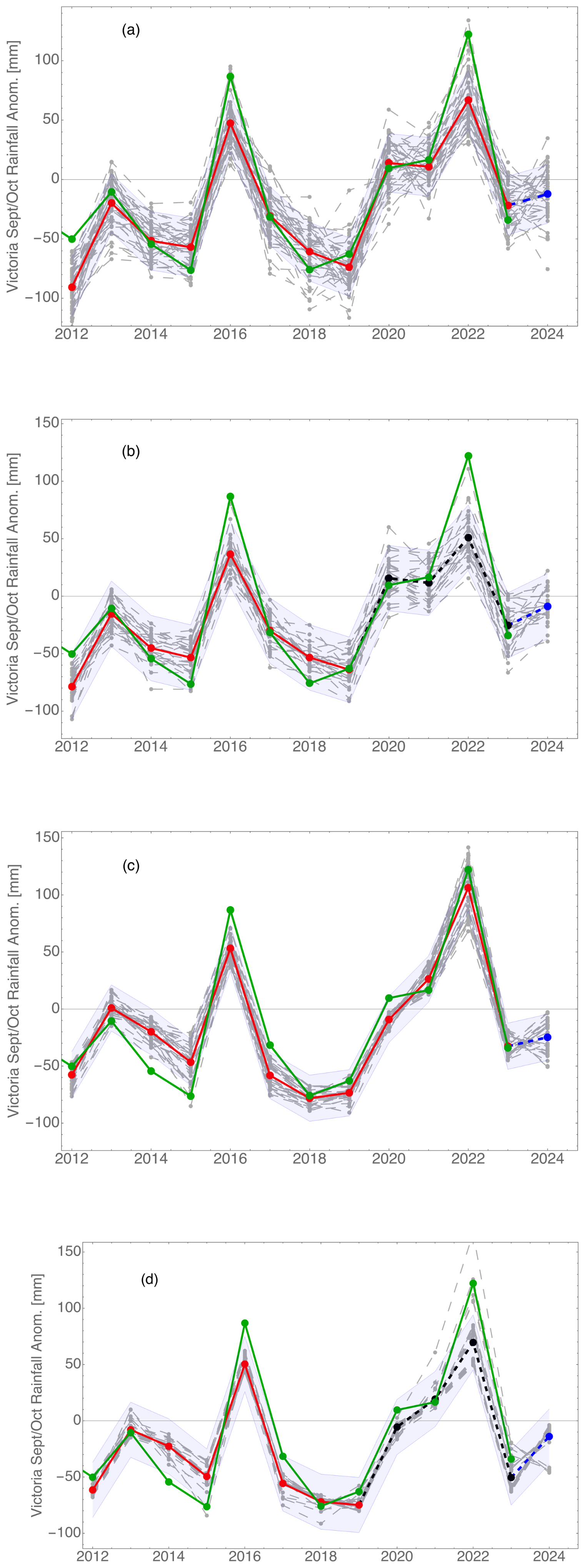
Figure 4 Hindcast and forecast of the rainfall anomaly in the state of Victoria during September and October using (a) June data, (b) June data with a test period (2020–2023), (c) July data, and (d) July data with a test period (2020–2023). Historic rainfall is shown in green, and mean values of the validation are shown in red. In this figure and all subsequent figures, points show monthly data, and lines are added to make year-to-year changes easier to follow. The 2024 forecast is the last point in blue. Faint dashed lines are the results from individual random network starts. The mean value of the RMSE over the period 2012–2023 is shown as shading. This and all subsequent hindcasts and forecasts use 2000–2024 data time series. In (b) and (d), only the data up to and including the year 2019 are used to define the network. Hindcast results using this network for the years 2020–2023 are shown in black, and the forecast for 2024 is shown in blue.

For the three studied regions, the RMSE values between the data and hindcast results are typically close to 20 mm. The RMSE values for each hindcast and forecast figure in the next section are shown as the grey uncertainty band. All numerical values of accuracy are shown in the table in Sect. S6.

3.4 Hindcasting and forecasting 2024 rainfall for three regions

Within the validation and hindcasting test periods, the three regions explored (Victoria, Murray–Darling Basin, and southeastern Australia) shared all of the main features of rainfall (see the map and correlation table in Sect. S1). During September and October, rainfall trends and anomalies appear to follow a single trend, possibly indicating a common physical origin. Using June or July data, hindcasting is fairly accurate, and I combine the two months into a single spring period. The behaviour and likely physical basis for November forecasting are different, and the predictions are less accurate. All rainfall anomalies were defined with respect to the 1991–2020 period, with combined September–October rainfall averages of 114.8, 73.4, and 108.5 mm for Victoria, the Murray–Darling Basin, and SE Australia, respectively. The corresponding November averages are 54.0, 47.1, and 51.5 mm, respectively.

With June data, forecasting is based on both the well-known drivers and the not commonly used drivers, the most important of which is the meridional gradient. Other prominent inputs are the Niño-3.4 area SST and IOD. SSTs over other regions of the Indian Ocean are sometimes helpful, as are land temperatures over Australia in the case of the Murray–Darling region. The years with extreme rainfall are underestimated. Including EOF expansion in the input data results in only a minor improvement. Partial agreement in the validation period requires four to six input streams, and the hindcasting success depends on details. While the results are sometimes unreliable, they still provide a reasonable indication of the developing trends.

With July data, the best predictor is the first Indian Ocean EOF (40° S to 20° N and 40 to 120° E). Adding just Niño-3.4 SSTs to the neural net inputs is already sufficient to provide good hindcasts. Further improvement is obtained by adding a few more input streams. The resulting July forecasts used are robust and insensitive to changes in the network structure or training details.

As a first example, in Fig. 4, we show rainfall hindcasts and a forecast for the state of Victoria. When hindcasting with June data, extreme-rainfall years are not fully anticipated. The learning rate during the training is set to be relatively high, resulting in a large scatter between individual runs but also more accurate mean values. In Fig. 4b and d, I show a test where the network is finalised with the data ending in 2017, thus reducing the validation set from 12 to 8 years. The accuracy of the result is moderately reduced, but the main features are unchanged.

With July data, it becomes possible to hindcast more extreme years, but some of the less important details are lost. Some years (2014–2015 or 2020) are presently impossible to hindcast accurately, but the errors are moderate.

Turning next to the important Murray–Darling Basin, the average errors are larger (Fig. 5), and forecasts are less reliable. Using July data, the very large anomalies in 2016 and 2022 are hindcast correctly, but the problem years of 2013 and 2020 are still inaccurate. In addition to ocean data, the inputs in panel (a) include temperatures on the Australian continent, whereas those in panel (b) are based on the first Indian Ocean EOF and Niño-3.4 data only.

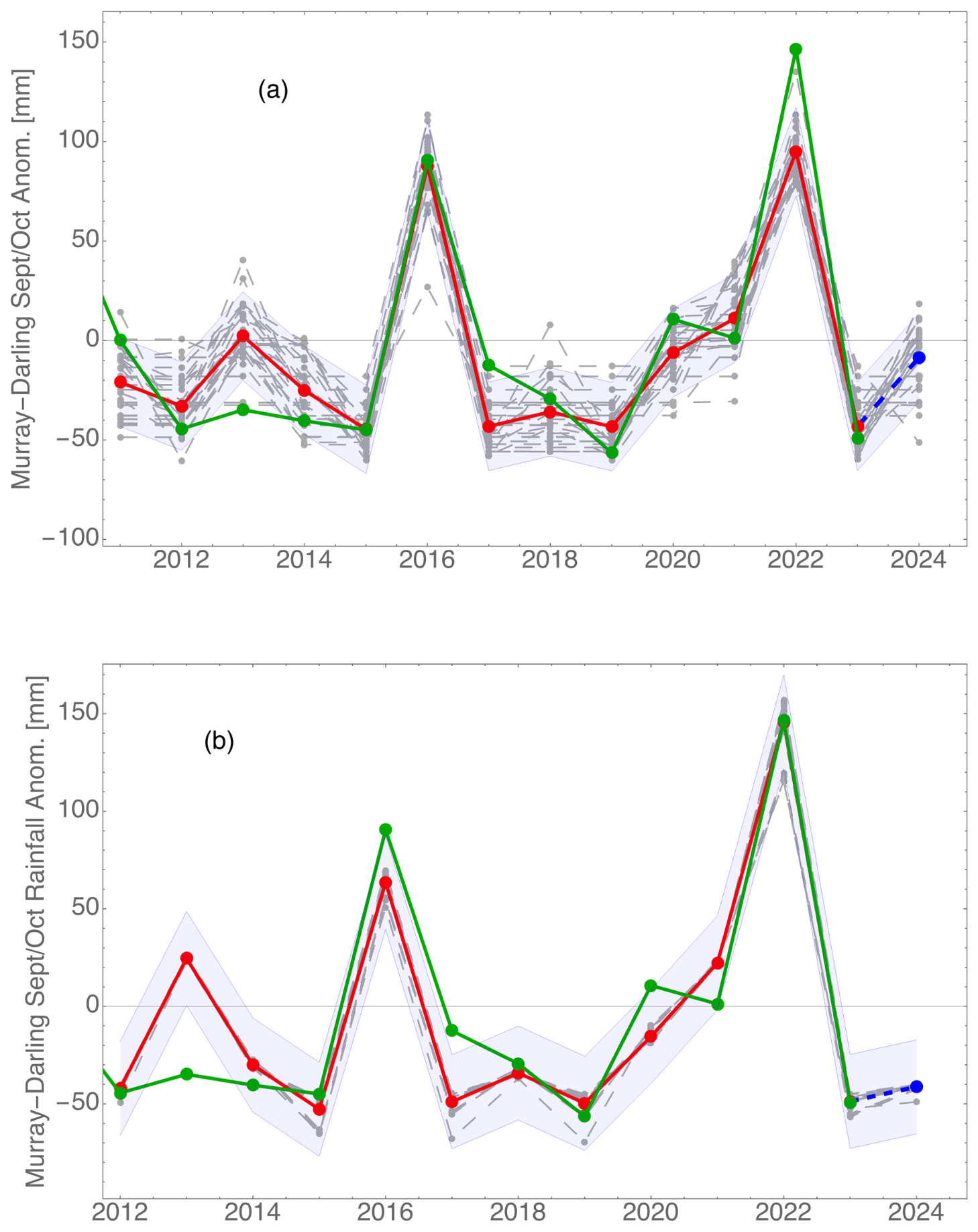
Figure 5 Murray–Darling Basin September–October rainfall hindcast and forecast using (a) June data or (b) July data. The symbols have the same meaning as in Fig. 4. In (a), setting a larger value for the network learning rate results in the system probing many states in search of the best solution. In (b), validation results were better with a low learning rate, when the system drifts to a local minimum without probing many adjacent states.

Hindcasting is most accurate for the larger SE Australia region (Fig. 6). The June data forecast shown in panel (a) is based on the Niño-3.4 SST, the meridional gradient, Australian continent temperatures, and Murray–Darling temperatures. The July forecast in panel (b) is based on the Indian Ocean EOF1 and Niño-3.4 SSTs. The hindcasts are similar in skill, but the errors appear at different places.

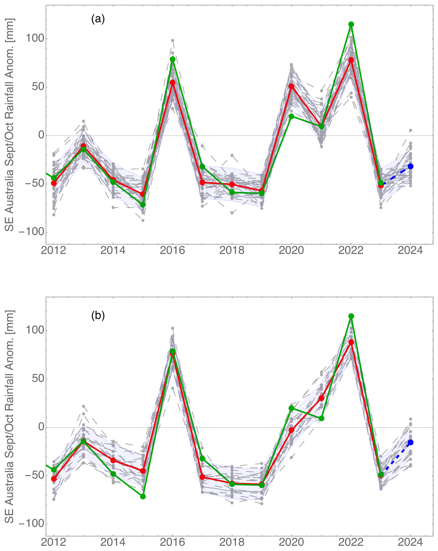
Figure 6 SE Australia September–October rainfall hindcast and forecast using (a) June data or (b) July data. The symbols have the same meaning as in Fig. 4.

Finally, we consider the rainfall in the November hindcast with the August data. For input data, the strong South Pacific Ocean feature visible in Fig. 1 is included as the second EOF (40° S to 5° N and 140° E to 100°) shown in Fig. 7. In addition, the inputs include the Niño-3.4 SST, several positions along the Pacific Ocean anomaly, the Indian Ocean meridional gradient, and the air surface pressure anomaly in Tahiti. The result shown in Fig. 8 appears to be reasonable, but only future forecasting will show if this combination is accurate and stable.

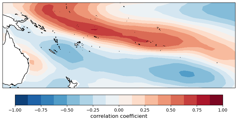
Figure 7 South Pacific EOF during the month of August corresponding to the configuration shown in Fig. 1 and used in forecasting November rainfall.

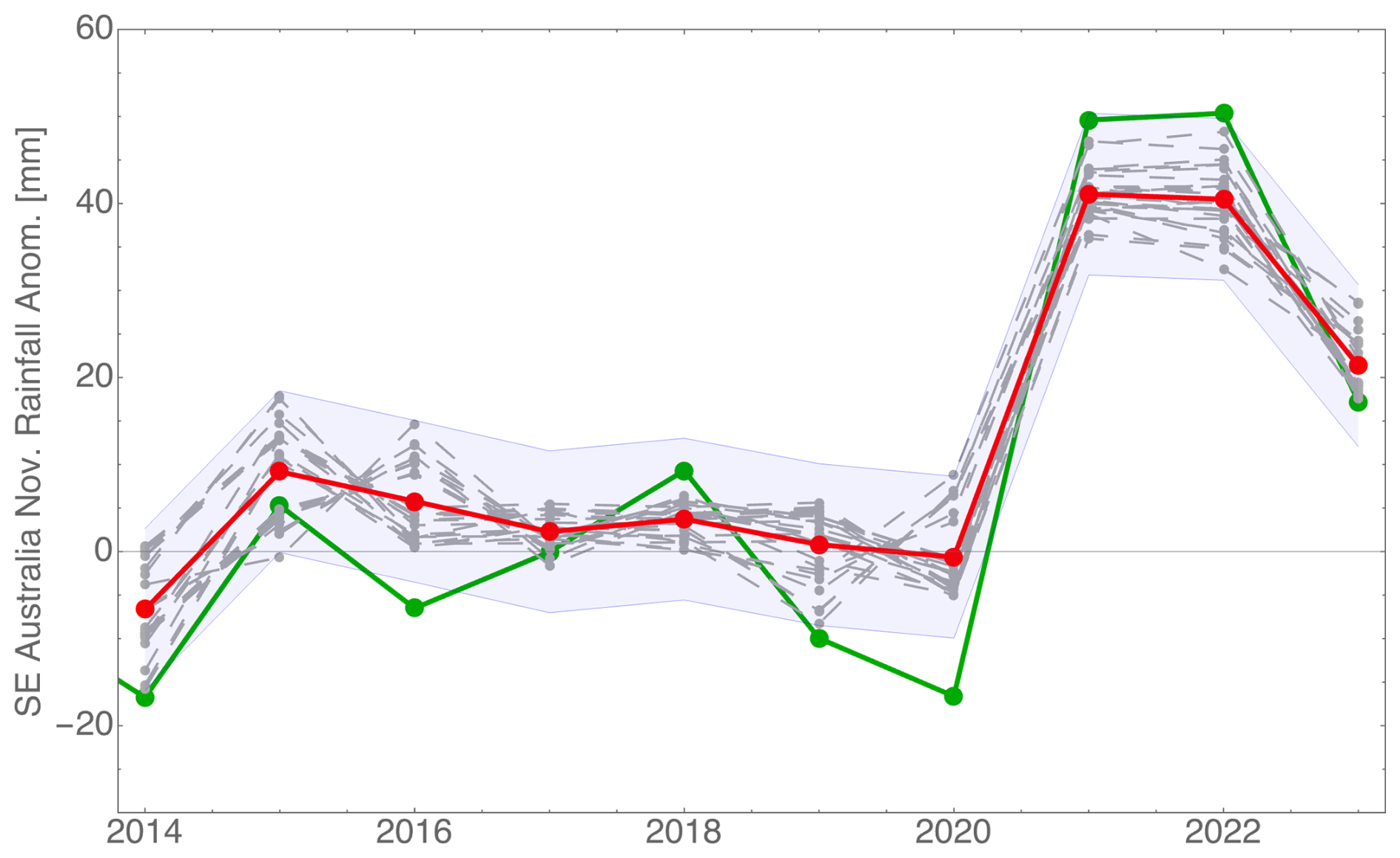
Figure 8 Hindcast of 2023 November rainfall in SE Australia evaluated with August data. The symbols have the same meaning as in Fig. 4.

Within the accessible months, during the training of neural networks, I encountered the well-known problem of overfitting the model when the datasets are small, and many adjustable parameters are available. This problem has a human analogue, which may arise when the investigator has a choice between many available possibilities for the input data and input parameters, eventually finding the set that fits in hindcasting tests. The forecasts where only a few predictor inputs are sufficient are less dependent on the input parameter choices and, hence, are preferable compared to the hindcasting fits with up to 10 different inputs. Since the selection of input data and training parameters has a large effect on the outcome, the following tests were always performed to explore the reliability of the results and the possible influence of overfitting resulting in unrealistic confidence. (1) The result must not depend strongly on the length of the validation segment. (2) Using training and validation data that end a few years earlier, e.g. in 2020, should still produce similar results (Fig. 4b and d). (3) The network learning rate should not have a strong influence on the result. My concern was largely allayed as forecasting with very different sets of inputs in the June–July data comparisons still led to similar outcomes in forecasting springtime rainfall.

4 Discussion

Ideally, throughout a year, a forecasting method should provide reliable forward information with only small errors. However, weather system development is ruled by chaotic dynamic equations, and, as shown first by Lorenz (1963) and elaborated upon in many further works, perfect forecasts are theoretically impossible because of the extreme sensitivity to initial conditions. The search described in Sect. 2 revealed strong correlations of different early indicators with rainfall during the spring months and weaker correlations at other times of the year. The rainfall during the winter months is only modestly correlated with SST, with accepted climate drivers, or with temperatures over different regions of the continent, with the correlation coefficients ranging from 0.2 to 0.4. This information is insufficient for the network architectures tested here, and forecasts had to be restricted to rainfall during the spring months. Data with a high correlation coefficient of approximately 0.70–0.75 (as is the case with the dominant EOF principal component in July) are much more valuable than data with a correlation coefficient of 0.60–0.65 (typical ocean indicators).

In the winter–spring period, the dominant physical modes are strong, the effective dimension of chaotic dynamics is not prohibitively high, and the neural network can forecast several months ahead with good skill. Particularly important is the ability of the method to make quantitative forecasts in difficult years with large anomalies, such as 2016 or 2022.

At less favourable times, the dominant modes are not as strong, and the behaviour is complex (ENSO predictability barrier; see, for example, Chen et al., 2020). If the chaotic dynamics of the physical processes cannot be followed for several months ahead, future rainfall will appear to be largely stochastic. Under such conditions, classical probabilistic forecasting using linear methods is favourable. Khastagir et al. (2022) tested both linear methods and neural networks in forecasting rainfall in W Australia and reported that linear methods tend to perform better.

In the winter–spring period studied in this work, conditions favour neural networks, and forecasting with linear regression was less accurate (results are in Sect. S7). When testing neural networks without the tanh nonlinearity, the results were not as good, particularly in the years of large deviations from the average (Sect. S7).

Neural network training performed in this work was conducted without any information about the physical significance or importance of each input data stream. In the longer term, we need to understand the physical mechanism driving climate fluctuations at annual and seasonal scales. It is hoped that the present identification of features that have a significant influence on rainfall during the following seasons may help in understanding the physical basis of the relationships between important climate variables and, thus, in advancing medium-term climate forecasting.