Interpretable seasonal multisite hidden Markov model for stochastic rain generation in France

We present a lightweight stochastic weather generator (SWG) based on a multisite hidden Markov model (HMM) trained on a large area with French weather station data. Our model captures spatiotemporal precipitation patterns with a strong emphasis on seasonality and the accurate reproduction of dry and wet spell distributions. The hidden states serve as interpretable large-scale weather regimes, learned directly from the data without requiring exogenous inputs. Compared to existing approaches, it offers a robust balance between interpretability and performance, particularly for extremes. The model architecture enables seamless integration of additional weather variables. Finally, we demonstrate its application to future climate scenarios, highlighting how parameter evolution and extreme event distributions can be analyzed in a changing climate.

1 Introduction

1.1 Context

The current context of climate change necessitates a careful analysis of industrial resilience in future climate conditions to anticipate adaptation needs. This includes estimating extreme hydrometeorological conditions, such as the frequency of long-lasting dry spells, which are critical for hydropower and nuclear generation. Parliamentary missions in France (Christophe and Pompili, 2018) have highlighted the need to quantify hydro-stress impacts on nuclear power generation. Similarly, understanding future hydrometeorological conditions is essential for farmers to develop robust agricultural strategies (see Pascual et al., 2017; Zhao et al., 2017; Parent et al., 2018, and references therein).

Rainfall can trigger natural hazards with diverse spatiotemporal characteristics, ranging from short-duration, localized intense showers to prolonged meteorological droughts affecting vast regions. As a result, precipitation modeling must be adapted to the specific hazard being addressed. Global and regional climate models can simulate the climate system and project its evolution under different forcing scenarios. However, they remain computationally expensive, limiting the number of simulations that can be performed. In practice, climate projections are made available in public repositories, such as the French national project DRIAS (Soubeyroux et al., 2021), which provides around 30 projections (see Sect. 8 for details). Yet, for accurate risk assessments, additional scenarios may be needed, leading to challenges in data augmentation and scenario resampling. Another limitation of climate models is their inability to fully capture local extremes, despite advancements in spatial resolution and process modeling (Luu et al., 2022). Consequently, stochastic weather generators remain widely used in impact studies. The recent IPCC Working Group 1 report of the 6th assessment (Arias et al., 2021) emphasizes the importance of such tools, stating that “Methodologies such as statistical downscaling, bias adjustment, and weather generators are beneficial as an interface between climate model projections and impact modeling and for deriving user-relevant indicators.” Unlike climate models, which represent the physical mechanisms governing climate evolution, stochastic weather generators are calibrated to reproduce the statistical properties of climate variables, including distributions, spatial and temporal correlations, and inter-variable dependencies in multivariate models.

Generating statistically coherent weather series in time and space is a challenging problem. Mathematically, these series form multivariate time-dependent data that are far from being independent and identically distributed. In simple terms, today's weather is strongly influenced by past conditions and spatial correlations with surrounding locations. Additionally, weather patterns evolve throughout the year and under climate change, making it essential to accurately reproduce both typical weather conditions and extreme events such as heavy precipitation and intense heatwaves.

For industries operating spatially scattered installations, a key concern is the simultaneous exposure of multiple facilities to the same extreme event. In electricity generation, prolonged, spatially extensive droughts can complicate grid management, making it crucial to assess their frequency to anticipate appropriate adaptation measures (International Energy Agency, 2022, e.g., Chap. 3 – Nuclear Power). Large-scale weather regimes can also significantly impact renewable energy production (van der Wiel et al., 2019). However, estimating the occurrence and intensity of such situations is not straightforward. Historical observations provide only a single realization among many possible trajectories influenced by climate variability. Climate models can expand the range of possible events but often fail to produce enough extreme cases for robust statistical analysis. For example, Lang and Poschlod (2024, Sect. 4.1) discuss an ensemble of 50 climate model simulations used to estimate return periods of heavy rainfall, while Fischer et al. (2023) show that an ensemble of 30 climate model simulations over 31 years each could not reproduce heatwaves of the same magnitude as the 2021 Pacific Northwest event. To address this limitation, they propose ensemble boosting methods to enrich simulations of extreme heatwaves. Stochastic weather generators (SWGs) offer a way to overcome this limitation by increasing the sample size, enabling better extreme event statistics at a manageable computational cost.

Beyond hazard modeling, stochastic weather generators are essential tools for climate stress testing (Robertson et al., 2007; Manzano and Ines, 2020; Ranger et al., 2022). By generating realistic large ensembles of weather simulations under a given climate scenario, they help decision-makers anticipate climate variability and implement proactive adaptation measures. Given the increasing impact of climate change, leveraging these models is crucial for building resilience and ensuring sustainability.

The purpose of this paper is to develop an interpretable parametric model that efficiently simulates spatially coherent rainfall patterns – both occurrences and amounts – across France, incorporating self-taught large-scale weather patterns. Unlike pure generative models based on neural networks (Goodfellow et al., 2014), the stochastic generator developed in this study benefits from easily interpretable parameters, enabling the incorporation of climate change factors (see Sect. 8.3). Recent studies (Miloshevich et al., 2024) compare the use of stochastic weather generators and deep learning models for extreme heatwave sampling, highlighting the complementary nature of these approaches. Other studies have shown that classical generative models are not adapted to learn heavy-tailed distributions (like rainfall), requiring specialized architecture dedicated to extremes (Allouche et al., 2022). Finally, enforcing physical constraints within such models remains a challenge, which is critical for generating long-term realistic weather simulations (Dueben and Bauer, 2018).

1.2 Background literature

Many stochastic weather generators are devoted to the generation of precipitation time series, as precipitation is a crucial variable for many impact studies in agriculture or hydrology. For reviews, see Wilks and Wilby (1999), Chen and Brissette (2014), Ailliot et al. (2015a), and Nguyen et al. (2023). Stochastic weather generator (SWG) development dates back to the 1980s, with the model proposed by Richardson (1981) to generate long samples of precipitation, minimum and maximum temperature, and solar radiation.

They can have different spatial scales, e.g., single-site models (Richardson, 1981), multisite models for closely located stations (Benoit et al., 2018), gridded-resolution models (Wilks, 2009; Dawkins et al., 2022), or models for widely separated stations (≳100 km) (Zucchini and Guttorp, 1991; Robertson et al., 2004). The temporal resolution can also vary, typically from sub-hourly (Cowpertwait et al., 2007) to hourly (Stoner and Economou, 2020) or daily rainfall amounts. Multisite daily stochastic generators will be the main focus of this work. A class of models focuses on nonparametric approaches, typically using resampling methods (e.g., Boé and Terray, 2008), which mix parametric and resampling techniques. The main drawback of these methods is that they cannot produce samples outside the observed distribution, limiting their usefulness for extreme value analysis. In such cases, parametric models are typically preferred.

The first important modeling choice is whether rain occurrence and rain amount should be generated separately. To simulate both rain occurrence and amounts simultaneously, one typically uses latent Gaussian variables, e.g., censored Gaussian latent variables (Bardossy and Plate, 1992; Ailliot et al., 2009; Baxevani and Lennartsson, 2015) and complex covariance structures (Flecher et al., 2010; Benoit et al., 2018; Bennett et al., 2018). These approaches conveniently model spatiotemporal dependencies within a common latent space using a covariance structure. They are highly flexible, allowing, for example, the easy inclusion of past dependence or other weather variables such as temperature. However, these approaches assume an underlying normal dependence, which is not always satisfied. Their computational complexity makes them very hard to train. Moreover, they tend to misrepresent dry and wet spells (e.g., Bennett et al., 2018, Fig. 4, or Baxevani and Lennartsson, 2015, Figs. 7 and 19), as they treat spatiotemporal dependence in rain occurrence and rain amounts the same way. One can argue that these are two distinct processes. In that case, modeling rain occurrences separately has typically been done using first-order Markov chains (Richardson, 1981), which can be easily extended to higher orders to better reproduce dry and wet spells (Srikanthan and Pegram, 2009). To model subsequent rain amounts, parametric distributions with light or heavy tails are used (see Chen and Brissette, 2014, for a comparison). In this second approach, addressing spatial dependence becomes challenging since it must be handled separately for rain amount and occurrence. To this end, a class of models referred to in this paper as WGEN models was proposed in Wilks (1998). It introduces a latent Gaussian copula to model correlations between rain occurrences at different sites. While this approach effectively reproduces pairwise correlations, it treats time and space dependence separately and, as we will show in Sect. 5.3, fails to capture large-scale, temporally persistent dry states.

Another option is to include spatial dependence using meteorologically defined weather types (e.g., dry, wet, or atmospheric circulation patterns), also referred to as weather regimes or circulation patterns. In this case, weather regimes are a finite set of large-scale patterns that characterize the weather of a given day. They can either be predefined and incorporated into the model as exogenous variables or inferred as latent variables; see Vaittinada Ayar et al. (2016) and Gutiérrez et al. (2019) for comparison of different approaches. For example, Vrac et al. (2007) identified weather types a priori through the classification of either precipitation data or exogenous atmospheric variables and trained a Markov-like precipitation model conditional on these inputs. Nguyen et al. (2024) applied a similar approach using a multivariate autoregressive model and a Gaussian latent model for rain occurrence and precipitation. Known dependence can also be incorporated using the generalized linear model (GLM) framework to make model parameters dependent on covariates such as previous-day dependence, known weather regimes, month of the year, and so on (see Yang et al., 2005; Chandler, 2020). See Holsclaw et al. (2016), Verdin et al. (2019), and Stoner and Economou (2020) for Bayesian versions of these GLM approaches. These approaches have two main drawbacks. First, they require selecting the relevant weather types or exogenous variables, along with the stochastic properties of precipitation conditional on weather types. See Philipp et al. (2016), Beck et al. (2016), and Huth et al. (2016) for comparisons and discussions on the impact of the choice of weather regimes based on synoptic variables. Additionally, Najibi et al. (2021) study the quality of a weather generator conditioned on different predefined weather patterns that were obtained by different methods. Second, the exogenous variables or weather regimes need to be specified by the user or accurately modeled in order to utilize the weather generator, which may pose limitations in certain applications.

To circumvent these difficulties, hidden Markov models (HMMs) introduce weather types as latent variables (Zucchini and Guttorp, 1991; Ailliot et al., 2009; Sansom and Thomson, 2010), which are directly inferred from the station and variable of interest without requiring additional data. This approach has the advantage of identifying weather regimes specifically adjusted to the weather characteristics of the area of interest (Najibi et al., 2021). The weather regimes are typically modeled using a latent Markov chain, and the distribution of the observations is conditioned on these latent states.

We may recall that it is not surprising from a probabilistic point of view that using latent variables to model complex dependencies might simplify analysis; see, for example, Kim et al. (2019) and Yamanishi (2023) for machine and deep learning reviews or Ghassempour et al. (2014) for time series clustering. In some very specific settings, it is even possible to prove that general exchangeable random variables can be realized as a mixture of product distributions (for some latent distribution) thanks to De Finetti's theorem (Diaconis and Freedman, 1980). In our setting, the exchangeability of the rain variables is not satisfied (e.g., rain occurrence probabilities differ at different weather stations); however, this case is still inspiring for modeling dependencies.

Coming back to multisite rain occurrence models, spatial HMMs have been proposed by Zucchini and Guttorp (1991), with the latent variable identified during inference shown to yield meaningful large-scale patterns (Robertson et al., 2004). In these papers, the main limitation is the conditional independence assumption, which states that multisite rain occurrences are independent given the weather states. This makes these generators suitable for widely separated stations where the assumption holds. In this paper, we adopt and verify this hypothesis a posteriori.

Other studies have incorporated exogenous weather variables into spatial HMMs to introduce more spatial correlations beyond those produced by the conditional independence assumption while also making them sensitive to other spatial phenomena. This is referred to in the literature as nonhomogeneous HMM (Hughes and Guttorp, 1994a, b; Hughes et al., 1999; Bellone et al., 2000; Greene et al., 2011) and used for statistical downscaling. As previously mentioned, selecting these additional dependencies is challenging and thus might not always be beneficial, as shown in Hughes and Guttorp (1994b, Table 4), where the authors, using an HMM-based model, compare a version with exogenous variables and one without. The conclusion is that the best model is the one without external forcing.

See Hughes and Guttorp (1994a) for a comparison of different model choices. In Kirshner (2005), the author provides an overview and tests different options for multivariate distributions, ranging from conditional independence to complex dependence structures, including tree structures.

Models incorporating spatial HMM conditional independence with rain amounts directly using exogenous variables have been explored (Bellone et al., 2000; Neykov et al., 2012; Holsclaw et al., 2016). In Kroiz et al. (2020), the model is first fitted under the conditional independence assumption without external variables, and then a Gaussian copula is applied conditional on the weather states to correlate rain amounts.

Finally, most approaches described above assume constant parameters over a period of interest, e.g., a month or a season. Therefore, time nonhomogeneity in the HMM, i.e., a transition matrix that depends on time, has also been proposed, for instance, to introduce wind diurnal cycles (Ailliot and Monbet, 2012; Ailliot et al., 2015b, or Touron, 2019a) for multivariate (temperature and precipitation) single-site HMM.

1.3 Our contribution

We introduce the seasonal hierarchical hidden Markov model (SHHMM), a lightweight seasonal model based on a hidden Markov model (HMM) for generating multisite and temporally realistic weather series, specifically precipitation. As in Touron (2019b), our model is fully time-nonhomogeneous, with parameters varying periodically throughout the year. The first layer consists of an autonomous spatial HMM for rain occurrences, similar to Zucchini and Guttorp (1991) and Robertson et al. (2004), while the second layer models multisite seasonal rainfall amounts conditioned on the learned hidden states.

1.3.1 Capturing large-scale dependencies

Our approach decomposes distributions using conditional independence with respect to hidden states, effectively capturing complex spatiotemporal dependencies without requiring external synoptic data. This ensures that large-scale weather regimes emerge naturally from the data. Moreover, they are shown to be robust across different station selections. To help with the station selection, we propose a simple metric to evaluate conditional independence. Rather than modeling rain amounts directly within the HMM, we focus on discrete rain occurrences. While previous attempts (Kroiz et al., 2020; Holsclaw et al., 2016) struggled to capture meaningful spatial correlations when including rain amounts in the hidden states, our results show that the inferred states remain interpretable and relevant for both rain occurrences and related meteorological variables such as mean sea level pressure. Unlike approaches that introduce additional spatial correlation structures (Hughes and Guttorp, 1994b; Kirshner et al., 2004), our model enforces conditional independence, ensuring that spatial dependencies are fully learned by the hidden states. This prevents ambiguity in model identification, where correlations could otherwise be absorbed by multiple components. Section 2.6 argues for the relevance of learning weather regimes with rain occurrences and conditional independence. In Sect. 2.5, the statistical identifiability of our model is discussed, showing in particular that a minimal number of stations is needed to be identifiable. Lastly, we propose a simple heuristic to initialize the SHHMM in the expectation maximization inference algorithm, which is known to be prone to local maxima (Cappé et al., 2005).

1.3.2 Improved temporal persistence and rainfall representation

To better reproduce wet and dry spell persistence, we introduce an additional autoregressive (local memory) Markov dependence (Cappé et al., 2005; Kirshner, 2005) to improve the simulation of spatiotemporal statistics. After generating rain occurrences, a Gaussian copula is used to conditionally add rain amounts, yielding significantly improved results over Kroiz et al. (2020). Our work contributes to the development of multisite SWGs for rainfall amounts, based on self-taught weather regimes, while explicitly decomposing the rain occurrence and amount processes.

1.3.3 Validation, comparison, and applications

We extensively validate the model's ability to reproduce key hydrometeorological statistics, including dry spell distributions and extreme rainfall accumulations. The model is compared with WGEN-type models (Wilks, 1998; Srikanthan and Pegram, 2009; Evin et al., 2018), which rely spatially on latent Gaussian structures and high-order Markov models locally. We show that our approach is more scalable in terms of complexity and better captures large-scale dry spells.

We also illustrate its usefulness in two climate-related applications: (i) estimating climate variability through multiple trajectory sampling, thereby showing how this can be used to compare climate models (used in IPCC reports) more accurately than with a single historical trajectory, and (ii) training our model on climate change scenarios and analyzing the evolution in terms of parameters and extremes.

Compared to existing multisite HMMs, our model uniquely combines local memory, seasonal parameter variation at low computational cost, and interpretable conditional rainfall generation. These properties make it suitable for studying large-scale risks such as prolonged droughts and extreme precipitation events, relevant in many applications.

Note that this multisite model generates weather data only at the training sites and hence cannot produce high-resolution fields. Nevertheless, multisite simulation remains highly useful in many operational contexts. For instance, in the energy sector, a critical question is the likelihood of prolonged dry spells affecting a large portion of the territory simultaneously. Such events can stress multiple power plants at once – particularly nuclear plants whose cooling systems depend on river flows, which are impacted by large-scale droughts. In this context, estimating the frequency of co-occurring dry episodes across regions is more relevant than reproducing detailed spatial variability. See Sect. 9 for a more detailed discussion on the perspective of this work. Similar challenges arise in large-scale agricultural production planning.

1.3.4 Software

The model and its code are available in the Julia package StochasticWeatherGenerators.jl (Métivier, 2024). It contains a reproducible step-by-step tutorial in its documentation describing all the data loading, training process, and simulations of the model described in this paper. Most figures in this paper can be exactly reproduced using the tutorial.

1.4 Organization of the paper

In Sect. 2, we describe the construction of the SHHMM. We explain in Sect. 3 the procedure to infer and select the model. Section 4 is entirely dedicated to the interpretation of the model parameters; in particular, the trained hidden states are interpreted as weather regimes for France and will be compared to other well-known weather regimes such as the North Atlantic Oscillation (NAO). In Sect. 5 we show simulation results for the spatiotemporal rain occurrence sequences with a special focus on extreme dry/wet sequences; we also compare our model to a WGEN-like model (Wilks, 1998). The actual rain amounts are then added on top of the previous model in Sect. 6 and tested in simulations in Sect. 7. In Sect. 8, we train our model with data from climate models on a reference historical period and on future climate change scenarios and discuss the results.

1.5 Notations used in the paper

For a positive integer M, we set $\left[\right[\mathrm{1}:M\left]\right]:=\mathit{\{}\mathrm{1},\mathrm{2},\mathrm{\dots },M-\mathrm{1},M\mathit{\}}$. If Θ is a finite set, $\left|\mathrm{\Theta }\right|$ denotes its cardinality. We make the distinction between t for a day and n for a date; see Sect. 2.2. The number of days is T=366.

2 Hidden Markov chain modeling

In this section, we introduce the statistical models considered in this work. The underlying mathematical framework is based on hidden Markov models (HMMs), which we develop and adapt with a focus on their application to stochastic weather generation.

2.1 Data

Daily rainfall observation time series are extracted from the European Climate Assessment & Dataset (ECA&D) (Klein Tank, 2002). We focus only on stations in France and close by. Among the available ECA&D weather stations in France and Luxembourg, 66 stations have 100 % valid data from 1 January 1956 to 31 December 2019, i.e., a 64-year range and, 23 376 data rows. We select S=10 of these stations in all of France (and Luxembourg): these weather stations are indexed with $s\in \mathcal{S}:=\mathit{\{}\mathrm{1},\mathrm{\cdots },S\mathit{\}}$.

This weather generator scales to the size of France and aims to capture large-scale, interpretable weather patterns. Hence, we select the stations to be as representative as possible of French weather. As explained in Sect. 2.2, where the conditional independence hypothesis is presented, the major limitation of the model is its requirement for some degree of independence between stations. In principle, we should define a criterion to optimize the selection of S=10 stations among the 66 available. Even with a simple approach, such as maximizing the mean distance between station pairs, the problem is computationally intractable, as there are $\left(\genfrac{}{}{0ex}{}{\mathrm{66}}{\mathrm{10}}\right)\simeq \mathrm{2}\times {\mathrm{10}}^{\mathrm{11}}$ possibilities. A more relevant yet even costlier criterion is the MSE_CI in Eq. (19) that is the mean square error (MSE) between observed and simulated rain occurrence correlations. To select 𝒮, we start with a reasonable initial configuration and iteratively perturb it by changing a few stations, retaining the set with the minimum MSE_CI. In Appendix C, we show that replacing 8 out of the 10 stations in 𝒮 with nearby ones does not affect the model's interpretation in terms of weather patterns. We show in Fig. 1 all the selected stations; in addition, we report in the heatmap scale the historical maximum of consecutive days without rain – dry spell – at each location. One of the goals of our modeling is to reproduce similar records. In Sect. 8, we will investigate how our model (and its parameters) evolves when historical data are replaced by future projection data according to some Representative Concentration Pathway (RCP) scenarios.

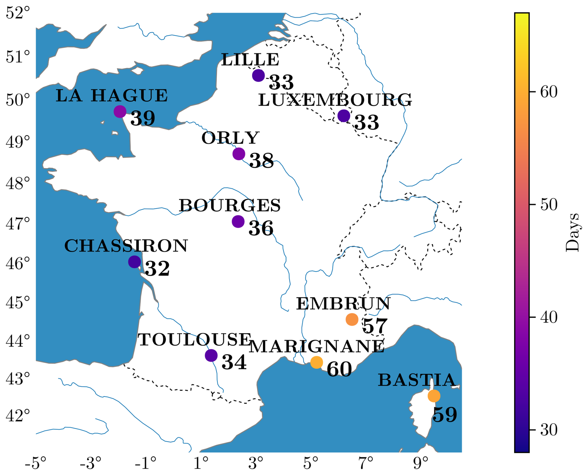
Figure 1 The 10 selected stations with their respective dry spell historical records over the period 1956–2019 (length in number of days).

The N=23 376 consecutive weather observations are labeled with $n\in \mathcal{D}:=\left[\right[\mathrm{1},N\left]\right]$. The multisite rain amount (MRA for short) is calculated as

$$\begin{array}{}\text{(1)}& R^{\left(n\right)}:=(R_{\mathrm{1}}^{\left(n\right)},\mathrm{\dots },R_S^{\left(n\right)})\in {\mathbb{R}}_{+}^S,\end{array}$$

for date n, where $R_s^{\left(n\right)}\left(\mathrm{mm}\right)$ is the daily rainfall amount at site s. Note that rainfall is measured in millimeters (mm) of depth typically using a rain gauge, which physically corresponds to a volume per unit area – that is, 1 mm of rainfall equals 1 L m⁻². It is the RR variable in the ECA dataset. Similarly, the multisite rain occurrence (MRO for short) is

$$\begin{array}{}\text{(2)}& Y^{\left(n\right)}:=(Y_{\mathrm{1}}^{\left(n\right)},\mathrm{\dots },Y_S^{\left(n\right)})\in \mathcal{I}:={\mathcal{I}}_s^S,\end{array}$$

where each $Y_s^{\left(n\right)}\in {\mathcal{I}}_s:=\mathit{\{}\mathrm{dry},\mathrm{wet}\mathit{\}}$, where dry means no rain and wet means nonzero rain, i.e., $R_s^{\left(n\right)}\ge \mathrm{0.1}\mathrm{mm}$ of daily cumulated rain.

In Sect. 4.1.2, to connect the weather patterns inferred by the model with physically meaningful atmospheric patterns, sea level pressure reanalysis data from the ERA5 reanalysis (Hersbach et al., 2020) are used. ERA5 is the latest climatic reanalysis produced by the ECMWF (European Centre for Medium-Range Weather Forecasts), providing hourly time series for various atmospheric, oceanic, and land surface parameters over the historical period from 1940 onward. It utilizes a 4D-Var data assimilation process to produce data on a 0.25° spatial resolution grid and is freely available on the Copernicus Climate Change Climate Data Store.

Lastly, in Sect. 8, two climate projections provided by the French climate service DRIAS (Soubeyroux et al., 2021), operated by Météo-France and Institut Pierre-Simon Laplace, are used. Developed to provide the best climate change information at the French national level for practitioners, DRIAS offers projections based on the Euro-CORDEX regionalization initiative, further statistically downscaled over France at an 8km resolution. A total of 42 simulations are available: 12 for the historical period (1951–2005) and 30 for the future (2006–2100), with 12 using the RCP8.5 scenario, 10 using RCP4.5, and 8 using RCP2.6. Among this set of projections, only two are used here, covering the historical period and the RCP8.5 scenario:

• CNRM-ALADIN63, regionalizing the CNRM-CM5 global climate model with the ALADIN63 regional climate model

• IPSL-WRF381P, regionalizing the IPSL-CM5A-MR global climate model with the Weather Research and Forecasting (WRF) regional climate model

The next subsections are devoted to the design of the model for the evolution of the MRO. The actual nonzero rain amount will be added on top of the model after it is trained in Sect. 6. Our approach relies on a hidden Markov model: generally speaking, it is made of a hidden component $\mathit{\{}{Z}^{\left(n\right)}:n\ge \mathrm{1}\mathit{\}}$ (that should be inferred) and of an observed one $\mathit{\{}{Y}^{\left(n\right)}:n\ge \mathrm{1}\mathit{\}}$ (here the MRO). All processes are discrete-time processes. See Cappé et al. (2005) for a general account about hidden Markov models.

2.2 Seasonal hidden Markov model (SHMM), model 𝒞₀

For the sake of clarity, we start with a simplified model, which will be extended hereafter. See Zucchini and MacDonald (2009) for an introduction to hidden Markov models for time series. Consider first the hidden component Z, common to all stations s∈𝒮: it can take discrete values in $\mathcal{K}:=\left[\right[\mathrm{1}:K\left]\right]$ that will be later interpreted as climate states for the region of interest, here France. We will thus refer to this variable as a weather regime (WR), as often done in the literature (e.g., van der Wiel et al., 2019). Note that other equivalent names also exist in the literature, such as weather types, weather patterns, or atmospheric circulation patterns.

The time evolution of $\mathit{\{}{Z}^{\left(n\right)}:n\ge \mathrm{1}\mathit{\}}$ follows a nonhomogeneous Markov chain on the state space 𝒦, with initial distribution $\mathit{\xi }=({\mathit{\xi }}_{\mathrm{1}},\mathrm{\cdots },{\mathit{\xi }}_K)$, i.e., ${\mathit{\xi }}_k=\mathbb{P}\left(Z^{\left(\mathrm{1}\right)}=k\right)$, and transition matrix ${\mathbf{Q}}_n\in {\mathbb{R}}^{K\times K}$ for n≥1,

$$\begin{array}{}\text{(3)}& {\mathbf{Q}}_n(k,k^{\prime })=\mathbb{P}\left(Z^{(n+\mathrm{1})}=k^{\prime }\mid Z^{\left(n\right)}=k\right).\end{array}$$

To fit the climate context, we assume that the transition matrix Q_n is a T-periodic function of n with T=366, i.e., ${\mathbf{Q}}_{n+T}={\mathbf{Q}}_n$; we will thus refer to the Markov chain as a seasonal Markov chain. In that case, we will distinguish between the label day of the year $t\in \mathcal{T}:=\left[\right[\mathrm{1}:T\left]\right]$ and the label full date n used to denote the position in the sequence. Each n corresponds to one t, but for each t there are as many date n∈𝒟 variables as the number of periods in the sequence: the matrices Q depend on time only through the day t. If T was equal to 1, this SHMM would be a regular homogeneous HMM, i.e., a constant matrix $\mathbf{Q}(k,k^{\prime })=\mathbb{P}\left(Z^{(n+\mathrm{1})}=k^{\prime }\mid Z^{\left(n\right)}=k\right)$ for all n∈𝒟 values. Next, we design the model for the time evolution of the MRO Y. The intuition behind the choice of well-spread stations is that local weather variables Y, conditional on weather regimes Z, are independent. In addition, we assume that the conditional distribution of Y⁽ⁿ⁾ does not depend on the past of Y and is also periodic. All is summarized in the following assumption.

(H-𝒞₀)

Z evolves as a seasonal Markov chain with period T=366. Conditional on the process $\mathit{\{}{Z}^{\left(n\right)}:n\ge \mathrm{1}\mathit{\}}$, the spatial components $Y_{\mathrm{1}}^{\left(n\right)},\mathrm{\dots },Y_S^{\left(n\right)}$ are independent and, furthermore, the conditional distribution of each $Y_s^{\left(n\right)}$ only depends on Z⁽ⁿ⁾. This is a Bernoulli distribution describing the probability of rain at a station s and date n, conditional on Z⁽ⁿ⁾=k: it is denoted as $f_{k,n,s}$ (called emission distribution in the HMM literature) and assumed to T-periodic, i.e., $f_{k,n+T,s}=f_{k,n,s}$, and thus represented as

$$\begin{array}{}\text{(4)}& \begin{array}{rl}{f}_{k,t,s}\left(y_s\right)& =\mathbb{P}\left(Y_s^{\left(n\right)}=y_s\mid Z^{\left(n\right)}=k\right)\\ & ={\mathit{\lambda }}_{k,t,s}{\mathbf{1}}_{y_s=\mathrm{wet}}+(\mathrm{1}-{\mathit{\lambda }}_{k,t,s}){\mathbf{1}}_{y_s=\mathrm{dry}}\end{array}\end{array}$$

for some parameters ${\mathit{\lambda }}_{k,t,s}\in [\mathrm{0},\mathrm{1}]$.

The above model for $\left\{\left(Z^{\left(n\right)},Y^{\left(n\right)}\right):n\ge \mathrm{1}\right\}$ is referred¹ to as 𝒞₀ and called a seasonal hidden Markov model (SHMM), with period T, initial distribution ${\mathit{\xi }}_{\cdot }=\mathbb{P}\left(Z^{\left(\mathrm{1}\right)}=\cdot \right)$, transition matrix Q_t, and distributions $f_{k,t,s}$. This SHMM terminology is borrowed from Touron (2019a).

The SHMM chain is illustrated in Fig. 2.

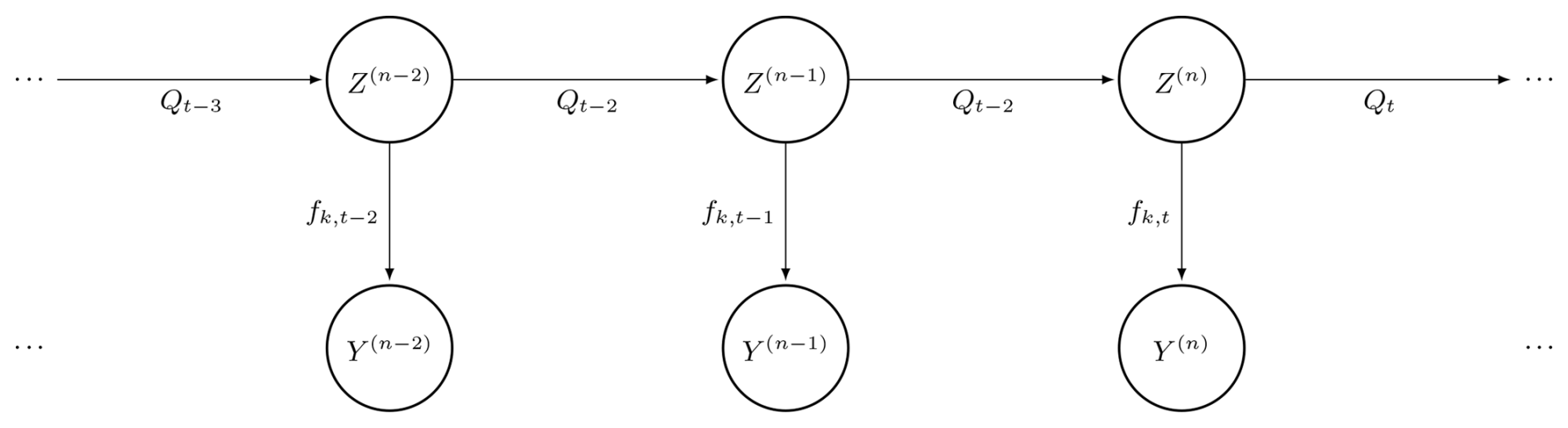
Figure 2 A seasonal hidden Markov process $(\mathit{\xi },{\mathbf{Q}}_{\mathrm{t}},f_{k,t}{)}_{k\in \mathcal{K},t\in \mathcal{T}}$, where Z represents the hidden variables (weather regimes), Y the observed multisite rain occurrence (MRO), Q the transition matrix, and f the distribution of the observations.

A few remarks before going further can be found below.

• This model accounts for leap years: for instance, the date $n=\mathrm{59}+\mathrm{366}=\mathrm{425}$ corresponds to 28 February 1957, i.e., to the day t=59, while the next date n=426, 1 March 1957, is the day t=61. All 29 February dates are labeled with t=60. With this convention, the estimation of parameters for t=60 will be performed with 3 times fewer data than for other dates; nevertheless, it will have a quite minor impact on the procedure because of the time smoothing of parameters discussed in Sect. 2.4.

• The annual periodicity of the distributions Q_t and $f_{t,k,s}$ is questionable. On the one hand, for obvious reasons of statistical inference, it is not possible to try to estimate as many distributions (parameterized by n∈𝒟) as there are data available, which leads to the reasonable assumption of annual stationarity as in Touron (2019b). On the other hand, annual stationarity is probably not accurate considering climate change. In our methodology, the calibrated parameters should be understood as valid over the data horizon used. We will see in Sect. 8 that shifting the data period into the future (using climate projection under different RCPs) will cause some parameters to evolve. Let us mention some tests in Touron (2019b, Chap. V) showing that the effect of climate change on precipitation is not easily identifiable (unlike for temperatures), supporting the stationarity hypothesis of our model. Including nonstationary effects with spatial HMM would require modifying the model to allow exogenous variables like in Bellone et al. (2000), Greene et al. (2011), and Dawkins et al. (2022) and will not be explored in this paper.

As a consequence of the spatial independence assumption in Sect. 2.2, the conditional likelihood of the MRO at date n is given by

$$\begin{array}{}\text{(5)}& f_{k,t}\left(y\right):=\mathbb{P}\left(Y^{\left(n\right)}=y\mid Z^{\left(n\right)}=k\right)=\prod _{s\in \mathcal{S}}{f}_{k,t,s}\left(y_s\right).\end{array}$$

This probability depends only on n by the corresponding day t. This assumption forces the model to learn spatial features (and spatial dependence) through the hidden states.

Later in this paper, we show (see Fig. B2) that this SHMM produces, in general, shorter dry or wet spells than the ones observed, suggesting that the Markov dynamics of the weather regime Z are not enough to stochastically explain the temporal evolution of the MRO Y. Indeed, Z is a weather regime over all of France and does not take into account the local dynamics of rain occurrence $Y_s^{\left(n\right)}$, i.e., that in addition to being influenced by the global weather, local weather should also be dependent on the local previous day's MRO $Y^{(n-\mathrm{1})},Y^{(n-\mathrm{2})},\mathrm{\cdots }$. Hence, it makes sense to define the dynamics of the MRO conditional on several previous days. This is the raison-d'être of the next models 𝒞_m and m>0.

We end this section with another set of remarks considering our model assumptions, which will also apply to 𝒞_m>0 models.

• The conditional independence hypothesis in Sect. 2.2 is discussed in Sect. 2.6.

• Note that conditional independence does not imply independence between stations. The model will learn, through the hidden states, “long-range correlation”, whereas conditional independence will mean that there is no short-range correlation. The actual correlations between the selected stations can be seen in Fig. 13 for MRO and range between 0 and ≃0.5.

• In Hughes and Guttorp (1994b, Fig. 3), the pairwise correlation conditional on hidden states (and synoptic forcing) is shown to decrease very quickly with distance. Typically, the characteristic decay length is around 50 km for most station pairs.

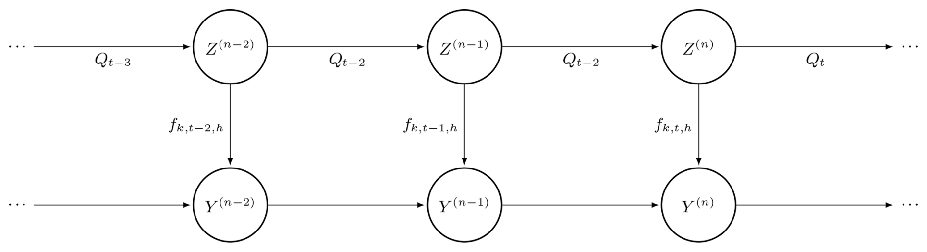
2.3 Seasonal hierarchical hidden Markov model (SHHMM), model 𝒞_m with m>0

To better reproduce the dry and wet spell distributions, we consider additional local conditioning. Different lengths of this additional local conditioning $Y_s^{\left(n\right)}\mid (Z^{\left(n\right)},Y_s^{(n-\mathrm{1})},Y_s^{(n-\mathrm{2})},\mathrm{\cdots },Y_s^{(n-m)})$ will correspond to different models 𝒞_m (with some memory parameter $m=\mathrm{1},\mathrm{2},\mathrm{\cdots }$). Intuitively, models with history 𝒞_m>0 should display better temporal persistence than the 𝒞₀ model' i.e., consecutive day sequence statistics should be replicated better. On the other hand, these models 𝒞_m>0 require more parameters to be fitted for the same number of data, and thus one should expect statistically less accurate estimates if m is too large.

Given m>0, we introduce the history variable

$$H^{\left(n\right)}:=(Y^{(n-\mathrm{1})},Y^{(n-\mathrm{2})},\mathrm{\cdots },Y^{(n-m)})\in {\mathcal{H}}^{\left(m\right)}:={\mathcal{I}}^m$$

and its local analog $H_s^{\left(n\right)}:=(Y_s^{(n-\mathrm{1})},Y_s^{(n-\mathrm{2})},\mathrm{\cdots },Y_s^{(n-m)})\in {\mathcal{H}}_s^{\left(m\right)}:={\mathcal{I}}_s^m$. The following hypothesis 𝒞_m summarizes the model.

(H-𝒞_m)

Z evolves as a seasonal Markov chain with period T=366. Conditional on the hidden variable $\mathit{\{}{Z}^{\left(n^{\prime }\right)}:n^{\prime }\ge \mathrm{1}\mathit{\}}$ and the local history H⁽ⁿ⁾, the spatial components $Y_{\mathrm{1}}^{\left(n\right)},\mathrm{\dots },Y_S^{\left(n\right)}$ are independent, and, furthermore, the conditional distribution of each $Y_s^{\left(n\right)}$ only depends on Z⁽ⁿ⁾ and $H_s^{\left(n\right)}$. This distribution is a Bernoulli distribution describing the probability of rain at a station s and date n, conditional on Z⁽ⁿ⁾=k and $H_s^{\left(n\right)}=h_s$: it is denoted as $f_{k,n,s,h_s}$, assumed to be T-periodic, and represented as

$$\begin{array}{}\text{(6)}& \begin{array}{rl}{f}_{k,t,s,h_s}& \left(y_s\right):=\mathbb{P}\left(Y_s^{\left(n\right)}=y_s\mid Z^{\left(n\right)}=k,H_s^{\left(n\right)}=h_s\right)\\ & ={\mathit{\lambda }}_{k,t,s,h_s}{\mathbf{1}}_{y_s=\mathrm{wet}}+(\mathrm{1}-{\mathit{\lambda }}_{k,t,s,h_s}){\mathbf{1}}_{y_s=\mathrm{dry}}\end{array}\end{array}$$

for some parameters ${\mathit{\lambda }}_{k,t,s,h_s}\in [\mathrm{0},\mathrm{1}]$ depending only on n by the associated day t, the hidden state k, and the m previous days' observation value h_s at the station s.

As a consequence, and similarly to Eq. (5),

$$\begin{array}{}\text{(7)}& \begin{array}{rl}{f}_{k,t,h}\left(y\right)& :=\mathbb{P}\left(Y^{\left(n\right)}=y\mid Z^{\left(n\right)}=k,H^{\left(n\right)}=h\right)\\ & =\prod _{s\in \mathcal{S}}{f}_{k,t,s,h_s}\left(y_s\right).\end{array}\end{array}$$

The 𝒞_m>0 models are defined by $(\mathit{\xi },{\mathbf{Q}}_{\mathrm{t}},f_{k,t,h}{)}_{k\in \mathcal{K},t\in \mathcal{T},h\in {\mathcal{H}}^{\left(m\right)}}$, where the law of the first observations ${\mathit{\xi }}_{\cdot }=\mathbb{P}\left(H^{\left(\mathrm{1}\right)}=\cdot ,Z^{\left(\mathrm{1}\right)}=\cdot \right)$, where $H^{\left(\mathrm{1}\right)}=(Y^{\left(\mathrm{0}\right)},\mathrm{\dots },Y^{(\mathrm{1}-m)})$ is added.

Regarding the usual terminology of hidden Markov chains, the model 𝒞₀ is a standard (periodic) HMM (Cappé et al., 2005, Sect. 2.2) since the observed variables $\mathit{\{}{Y}^{\left(n\right)}:n\ge \mathrm{0}\mathit{\}}$ are independent given the hidden variables $\mathit{\{}{Z}^{\left(n\right)}:n\ge \mathrm{0}\mathit{\}}$. For other models ${\mathcal{C}}_{\mathrm{1}},{\mathcal{C}}_{\mathrm{2}},\mathrm{\cdots }$, because of the dependence with respect to previous days through $Y^{(n-\mathrm{1})},Y^{(n-\mathrm{2})},\mathrm{\cdots }$, we are rather in the presence of autoregressive HMMs as described in Kirshner (2005, Sect. 3.1.1) (also discussed in Cappé et al., 2005, Sect. 2.2.3, under the name hierarchical HMMs): conditional on $\mathit{\{}{Z}^{\left(n\right)}:n\ge \mathrm{0}\mathit{\}}$, the MRO process $\mathit{\{}{Y}^{\left(n\right)}:n\ge \mathrm{0}\mathit{\}}$ evolves as a Markov chain with memory m. This is a significant difference from other precipitation models in the literature, such as Touron (2019a), Holsclaw et al. (2016), and Kroiz et al. (2020).

In the remainder of the article, we will use the term seasonal hierarchical hidden Markov model (SHHMM) to refer to the model 𝒞_m>0. Note that we will also use the same term to describe the full model, i.e., 𝒞_m>0 with added rainfall amounts (see Sect. 6).

We illustrate the 𝒞_m=1 model in Fig. 3.

Figure 3 Illustration of a seasonal hierarchical hidden Markov model with 1 d memory m=1.

Note that a time-independent autoregressive HMM was proposed in the PhD work of Kirshner (2005, Sect. 6.1.1) as a promising option but, to the best of our knowledge, has not been explored further. However, the combination of HMM with local memory, seasonality (see Sect. 2.4), and the subsequent addition of rainfall amount (see Sect. 6) appears to be new.

2.4 Hypothesis and modeling of the time regularity of parameters

The previous models 𝒞₀ and 𝒞_m>0 depend on the T-periodic functions $({\mathbf{Q}}_{\mathrm{t}},f_{k,t,h}{)}_{k\in \mathcal{K},h\in {\mathcal{H}}^{\left(m\right)}}$. A quick inspection of the number of scalar parameters to estimate on each day t∈𝒯 gives

• K(K−1) coefficients for the transition matrix Q_t and

• $K\times S\times {\mathrm{2}}^m$ coefficients for the Bernoulli distribution parameter ${\mathit{\lambda }}_{k,t,s,h_s}$ for all $k,s,$ and h_s.

For S=10, K=4, and m=1, it gives 92 scalar parameters, which is larger than the number of available data at each day t (64 for usual days and 16 for 29 February). On the one hand, estimating the parameters by maximizing the observed likelihood independently at each day t∈𝒯 is conceptually simple. On the other hand, the estimated parameters would suffer from high variance as there are too few data at each day t. Therefore, in the inference procedure that will be exposed in Sect. 3, a time regularity constraint will be imposed. This procedure (detailed later) will be essential to recover interpretable and meaningful results.

Let us argue in more detail. Intuitively, the timescale of variation of the model parameters should be of the order of magnitude of a month (30 d). Hence, once fitted, the parameters should evolve as a smooth function of day t. The advantages of imposing a smoothing are multiple:

1. This avoids unrealistic, erratic day-to-day changes in the parameters while allowing for a physically realistic seasonal evolution.

2. It helps to overcome the lack of data at each day t; indeed, the smoothing implies that the data from neighboring days $t-\mathrm{1},t+\mathrm{1},t-\mathrm{2},t+\mathrm{2},\mathrm{\dots }$ are accounted for when making an inference at day t.

3. In terms of identifiability of the model, it is well-known that HMMs are identifiable up to relabeling of the hidden states. In the case of SHMM, the model is not identifiable up to the relabeling of hidden states at each day t (Touron, 2019a). Thus, it is very likely that a naive likelihood optimization routine gives quite different parameters on consecutive days, whereas for obvious interpretability reasons, we seek a smooth evolution as a function of the day t of the calendar year.

A popular choice in the literature is to use trigonometric polynomials (Langrock and Zucchini, 2011; Papastamatiou et al., 2018; Touron, 2019b) to parameterize the parameters as a function of the day t∈𝒯 (see Eqs. 8–9b below) and directly infer new parameters. The final SHMM or SHHMM is then only identifiable up to a global relabeling common to all t. Other methods, such as cyclic penalized splines (Feldmann et al., 2023; Dawkins et al., 2022), could have been considered. Thus, each parameter $({\mathbf{Q}}_{\mathrm{t}},{\mathit{\lambda }}_{k,t,s,h_s}{)}_{k\in \mathcal{K},s\in \mathcal{S},h\in {\mathcal{I}}_s}$ is composed with the trigonometric polynomial as follows: given some coefficients $c_{\mathrm{0}},c_{\mathrm{1}},\mathrm{\dots }$, set

$$\begin{array}{}\text{(8)}& P_c\left(t\right):=c_{\mathrm{0}}+\sum _{d=\mathrm{1}}^{\mathrm{Deg}}\left(c_{\mathrm{2}d-\mathrm{1}}\cos \left({\displaystyle \frac{\mathrm{2}\mathit{\pi }d}{T}}t\right)+c_{\mathrm{2}d}\sin \left({\displaystyle \frac{\mathrm{2}\mathit{\pi }d}{T}}t\right)\right)\end{array}$$

for some degree Deg. For all k∈𝒦 the transition matrices are given by

$$\begin{array}{}\text{(9a)}& \begin{array}{rl}{\mathbf{Q}}_{\mathrm{t}}(k,l)& ={\displaystyle \frac{e^{P_{c_{k,l}}\left(t\right)}}{\mathrm{1}+{\sum }_{l=\mathrm{1}}^{K-\mathrm{1}}{e}^{P_{c_{k,l}}\left(t\right)}}}\text{for}\mathrm{1}\le l<K,\\ & {\mathbf{Q}}_{\mathrm{t}}(k,K)={\displaystyle \frac{\mathrm{1}}{\mathrm{1}+{\sum }_{l=\mathrm{1}}^{K-\mathrm{1}}{e}^{P_{c_{k,l}}\left(t\right)}}},\end{array}\end{array}$$

and the Bernoulli parameters in Eqs. (4)–(6) by

$$\begin{array}{}\text{(9b)}& {\mathit{\lambda }}_{k,t,s,h_s}={\displaystyle \frac{\mathrm{1}}{\mathrm{1}+e^{P_{c_{k,s,h_s}}\left(t\right)}}}.\end{array}$$

The parameterization of Q_t corresponds to the log-ratio transformation well-known in compositional data analysis (Pawlowsky-Glahn and Buccianti, 2011). These definitions ensure $\mathrm{0}<{\mathit{\lambda }}_{k,t,s,h_s}<\mathrm{1}$, $\mathrm{0}<{\mathbf{Q}}_{\mathrm{t}}<\mathrm{1}$ and ${\sum }_{l\in \mathcal{K}}{\mathbf{Q}}_{\mathrm{t}}(k,l)=\mathrm{1}$, $\forall t\in \mathcal{T}$, and $\forall k\in \mathcal{K}$. A model with a high degree Deg will be able to capture shorter and shorter sub-seasonal/monthly/sub-monthly phenomena.

A quick inspection of the number of parameters (the coefficients c) gives (for S=10, K=4, m=1, and Deg=1 corresponding to roughly four seasons) $\mathrm{92}\times \mathrm{3}=\mathrm{276}$ scalar parameters (for all t∈𝒯) instead of $\mathrm{92}\times \mathrm{366}=\mathrm{33}\mathrm{672}$ in the previous day-by-day parameterization. The gain is quite significant. However, the maximization step has no analytical solutions: the subsequent numerical optimization is heavy because now $({\mathbf{Q}}_{\mathrm{t}},{\mathit{\lambda }}_{k,t,s,h_s}{)}_{k\in \mathcal{K},s\in \mathcal{S},h\in {\mathcal{I}}_s}$ is not independent with respect to t∈𝒯. The resulting parametric problem is of lower dimensions but more complex to solve than the T individual problems.

In the rest of the paper, we denote by θ all the coefficients appearing in Eqs. (8)–(9b), and those are to be optimized:

$$\begin{array}{}\text{(10)}& \begin{array}{rl}\mathit{\theta }& :=\mathit{\{}{c}_{k,l}\in {\mathbb{R}}^{\mathrm{2}\mathrm{Deg}+\mathrm{1}},c_{k,s,h_s}\in {\mathbb{R}}^{\mathrm{2}\mathrm{Deg}+\mathrm{1}}:\\ & k\in \mathcal{K},l\in \left[\right[\mathrm{1}:K-\mathrm{1}\left]\right],s\in \mathcal{S},h_s\in {\mathcal{I}}_s\mathit{\}}.\end{array}\end{array}$$

2.5 Identifiability

For the inference problem to make sense, the model must be identifiable. Latent models are known to be only identifiable up to label swapping. Moreover, Bernoulli mixtures are known to be non-identifiable (Gyllenberg et al., 1994). However, they are identifiable under a weaker notion of generic identifiability up to label swapping if the following condition holds (Allman et al., 2009, Corollary 5):

$$\begin{array}{}\text{(11)}& \mathrm{2}⌈{\log }_{\mathrm{2}}\left(K\right)⌉+\mathrm{1}\le S.\end{array}$$

Generically identifiable (Allman et al., 2009) implies in particular that the set of points for which identifiability does not hold has measure zero. Hence, for the applications, this notion is enough. For our application, we explore K being at most 8 so that S≥7.

In Touron (2019a, Theorem 1), the identifiability up to label swapping of the seasonal hidden Markov model is proven under the following assumptions.

1. For $\mathrm{1}\le t\le T$, the transition matrices ${\mathbf{Q}}_t^{\ast }$ are invertible and irreducible.

2. The matrix ${\mathbf{Q}}_{\mathrm{1}}^{\ast }\mathrm{\dots }{\mathbf{Q}}_T^{\ast }$ is ergodic, and its unique stationary distribution ξ^∗ is the distribution of Z⁽¹⁾.

3. For each $t\in \left[\right[\mathrm{1},T\left]\right]$, the K distributions $\left({\mathit{\nu }}_k^{\ast }\right(t){)}_{k\in \mathit{\{}\mathrm{1},\mathrm{\dots },K\mathit{\}}}$ are linearly independent.

The star (∗) denotes the set of true parameters. The irreducibility and ergodicity are satisfied under the parametric assumption for Q_t since all the matrix coefficients are strictly positive. The invertibility of Q_t is proven to hold up to a negligible set of parameters (Touron, 2019a, Sect. 2.4.1) for our parametric choice. The second condition can be shown using the coefficients of Q_t as strictly positive, so those of ${\mathbf{Q}}_{\mathrm{1}}^{\ast }\mathrm{\dots }{\mathbf{Q}}_T^{\ast }$ are also, and therefore ${\mathbf{Q}}_{\mathrm{1}}^{\ast }\mathrm{\dots }{\mathbf{Q}}_T^{\ast }$ is irreducible and aperiodic. To prove that the third assumption is satisfied in our case, we use the equivalence (Yakowitz and Spragins, 1968, Theorem Sect. 3) between linear independence of K distributions (ν_k)_k∈𝒦 and the identifiability of the mixture $\sum w_k{\mathit{\nu }}_{k,t}^{\ast }$ for some weights (w_k)_k∈𝒦. Together with the condition in Eq. (11), it follows that the model 𝒞_m=0 is generically identifiable up to a global relabeling. For higher-order models 𝒞_m>0, the local memory (autoregressive structure) of the distribution prevents direct application of the previous results; however, one can reasonably expect a similar condition to hold.

2.6 Model justification

We end the modeling section with a discussion on our choice of having inferred weather regimes using rain occurrences only.

Training hidden state models with binary variables such as wet/dry is well-established in machine learning classification techniques (see Bishop, 2006). Hence, rather than using a complex distribution (rain amount) in the HMM, we first focus on discrete rain occurrences, as in a Bernoulli mixture. Discrete distributions might seem like a simplification compared to existing methods, where rain amounts are directly expressed as a mixture of an atomic and continuous distribution (Touron, 2019a) or modeled using censored Gaussian distributions (Ailliot et al., 2009; Baxevani and Lennartsson, 2015), or in the context of Markov switching models where complex weather variables are modeled (Ailliot and Monbet, 2012; Ailliot et al., 2015b; Monbet and Ailliot, 2017; Ailliot et al., 2020). However, it can be argued that rain occurrences and amounts are very distinct processes with different statistical properties (Wilks, 1998; Dunn, 2004; Yang et al., 2019). For example, Vaittinada Ayar et al. (2020) use a spatial censored latent Gaussian model (conditioned on predefined weather regimes, but that is not the point) with the rain amount R directly. Hence, it assumes the same spatial correlation coefficient for the variables R>0 and Y. Similarly, while in our model we induce autoregressive Markov local memory for rain occurrences Y, their model assumes temporal memory using a MAR(1) model for R.

As mentioned previously, attempts to directly include spatial rain amounts within the hidden states have not been completely satisfactory in terms of learned correlations (e.g., Kroiz et al., 2020, Fig. 1, Ailliot et al., 2009, Model Cγ, or Holsclaw et al., 2016), where no correlation check seems to have been performed. Our approach produces fully interpretable hidden states that are relevant not only for rain occurrence but also for other variables such as rain amounts and mean sea level pressure. This is made possible by our assumption described in Sect. 2.2, which is both a strength and a limitation of the model: it requires a sparse station distribution but forces the hidden states to learn spatial patterns with temporal Markov dependence. Hence, at smaller scales (or for a denser station distribution), this assumption might not hold, and other, often less interpretable, methods may be required.

In fact, we argue that more complex HMMs can be increasingly difficult to train and lack interpretability. See Pohle et al. (2017) and de Chaumaray et al. (2023) for discussions on how imperfect parametric distributions can, for example, lead to an overestimation of the number of hidden states. For instance, extreme precipitation events often fall outside the reach of standard parametric rain distributions and could affect the weather regimes. Hence, learning hidden states directly from rain amounts might affect their quality. Moreover, a higher number of states could be necessary, but this would come at the expense of robustness since they are identified from the same amount of data. The choice of Bernoulli distributions for binary variables is, however, exact, suggesting that our model will likely pick a smaller number of hidden states, i.e., more interpretable.

Moreover, we also argue that breaking conditional independence, as in Hughes and Guttorp (1994b) and Kirshner et al. (2004) (which are the only two attempts we found in that direction), must be done carefully, as it complicates model identification. Specifically, spatial correlation can either be learned by the hidden states or by the added correlation structure. The proportion of dependence captured by each component is not explicitly controlled, and in some cases, all correlations may be learned through the additional correlation structure, rendering the hidden states irrelevant. Enforcing conditional independence in our model ensures that all spatial dependencies are learned exclusively by the hidden states and is validated a posteriori (see Sect. 5.2.2). In addition, the complexity of models like that in Hughes and Guttorp (1994b) is such that it is not clear how many more stations could be added (with respect to the conditional independence model) before reaching computational limits.

3 Fitting the SHHMM and selecting the hyperparameters

In Touron (2019a), the maximum likelihood estimator is shown to be a consistent estimator for the seasonal HMM, i.e., 𝒞_m=0. Proving the consistency for the autoregressive model 𝒞_m>0 is outside the scope of this paper; however, we will still use the maximum likelihood estimator to infer the model parameters.

Maximizing the likelihood of a latent model is usually done with the expectation maximization (EM) algorithm. See McLachlan and Krishnan (2007) for a general review of the EM algorithm and its extensions. To maximize the log-likelihood of the SHHMM, we will use a heterogeneous version of the Baum–Welch algorithm, which is a special kind of EM algorithm for hidden Markov models. The details of the algorithm can be found in Appendix E. Note that in this paper, we do not consider Bayesian inference as in Stoner and Economou (2020) and Verdin et al. (2019). Hence, the estimated parameters will be deterministic, and the resulting SWG model will solely be responsible for the climate variability, i.e., the uncertainty in the parameters' estimation will not be accounted for. A known issue of EM algorithms is that they can converge to local maxima. As we will illustrate, a naive random initialization of the algorithm without a good guess will likely land in some meaningless local maxima – even if multiple random initial conditions are tried – and/or take a very long time to converge.

Hence, before fitting SHHMM with the Baum–Welch algorithm, we will first find a crude estimator of the SHHMM by solving many simpler subproblems by using the procedure described below.

3.1 Initialization: the slice estimate

The idea is to first treat the MRO observations of each day of the year t∈𝒯 separately. On each day t, the distributions $\mathit{\{}{\stackrel{\mathrm{̃}}{f}}_{\mathrm{1},t},\mathrm{\cdots },{\stackrel{\mathrm{̃}}{f}}_{K,t}\mathit{\}}$ form a mixture model that can be fitted with a standard EM algorithm. Once this is done, we relabel the hidden state at each day t to ensure some continuity in the estimated parameters ${\stackrel{\mathrm{̃}}{\mathit{\theta }}}_{k,t,h,s}$. Finally, by identifying the most likely a posteriori states on each date n, we obtain an estimated sequence, $\mathit{\{}{\stackrel{\mathrm{̃}}{z}}^{\left(n\right)}:n\in \mathcal{D}\mathit{\}}$, which we use to fit the transition matrices $\widehat{Q}\left(t\right)$. The whole procedure is described in Appendix F. In Appendix F7, we show the gain in terms of likelihood and number of iterations when using the slice estimate compared to random initialization.

3.2 Baum–Welch algorithm for SHHMM

In the previous section, we provide an estimated SHHMM that we will use as a starting point in the Baum–Welch algorithm. The algorithm alternates between estimation (E) and maximization (M) steps to converge to a local maximum of the observed likelihood defined for the SHHMM $(\mathit{\xi },{\mathbf{Q}}_{\mathrm{t}},f_{k,t,h}{)}_{k\in \mathcal{K},t\in \mathcal{T},h\in {\mathcal{H}}^{\left(m\right)}}$ with m≥1 (see Sect. 2.3) by

$$\begin{array}{}\text{(12)}& \begin{array}{rl}\mathcal{L}\left(y^{(\mathrm{1}:N)};\mathit{\theta }\right)& =\mathbb{P}\left(Y^{(\mathrm{1}:N)}=y^{(\mathrm{1}:N)}\right)\\ & =\sum _{z^{\left(\mathrm{1}\right)},\mathrm{\dots },z^{\left(N\right)}\in {\mathcal{K}}^N}{\mathit{\xi }}_{z^{\left(\mathrm{1}\right)},h_{\mathrm{1}}}{f}_{z^{\left(\mathrm{1}\right)},t_{\mathrm{1}}}\left(y^{\left(\mathrm{1}\right)}\mid h^{\left(\mathrm{1}\right)}\right)\\ & \prod _{n=\mathrm{2}}^N{\mathbf{Q}}_{t_n}(z^{(n-\mathrm{1})},z_n)f_{z_n,t_n}\left(y^{\left(n\right)}\mid h^{\left(n\right)}\right),\end{array}\end{array}$$

where for sake of simplicity we assume that h₁ is known so that ${\mathit{\xi }}_{z_{\mathrm{1}},h_{\mathrm{1}}}=\mathbb{P}\left(Z^{\left(\mathrm{1}\right)}=z_{\mathrm{1}},H^{\left(\mathrm{1}\right)}=h_{\mathrm{1}}\right)=\mathbb{P}\left(Z^{\left(\mathrm{1}\right)}=z_{\mathrm{1}}\right)$. Note that this is the case in practice, as we have a few extra days of data to define h₁. We briefly detail each step of the EM algorithm in Algorithm 1, and more details can be found in Appendix E.

Algorithm 1 EM algorithm for SHHMM 𝒞_m.

Result: A SHHMM $(\mathit{\xi },{\mathbf{Q}}_{\mathrm{t}},f_{k,t,h}{)}_{k\in \mathcal{K},t\in \mathcal{T},h\in {\mathcal{H}}^{\left(m\right)}}$ with parameters ${\widehat{\mathit{\theta }}}^{\left(i_{\text{stop}}\right)}$.

Initialization:

An initial set of parameters θ⁽⁰⁾ is given, as mentioned, we use the Slice Estimate SHHMM described in Sect. 3.1.

Step (i>0):

E-step: Compute the smoothing probabilities

${\mathit{\pi }}_{n\mid N}^{{\mathit{\theta }}^{\left(i\right)}}\left(k\right)={\mathbb{P}}_{{\mathit{\theta }}^{\left(i\right)}}\left(Z^{\left(n\right)}=k\mid Y^{(\mathrm{1}:N)}\right)$ and ${\mathit{\pi }}_{n,n+\mathrm{1}\mid N}^{{\mathit{\theta }}^{\left(i\right)}}(k,l)={\mathbb{P}}_{{\mathit{\theta }}^{\left(i\right)}}\left(Z^{\left(n\right)}=k,Z^{(n+\mathrm{1})}=l\mid Y^{(\mathrm{1}:N)}\right)$ under the current parameter θ⁽ⁱ⁾. These probabilities can be computed using the Forward-Backward procedure (Appendix E).

M-step: Maximize the function $\mathcal{R}(\mathit{\theta },{\mathit{\theta }}^{\left(i\right)})={\mathbb{E}}^{{\mathit{\theta }}^{\left(i\right)}}\left[\log \mathcal{L}\left(Y^{(\mathrm{1}:N)},Z^{(\mathrm{1}:N)};\mathit{\theta }\right)\mid Y^{(\mathrm{1}:N)}\right]$ with respect to θ.

Stop:

The iterations stop at i=i_stop when $\mathcal{L}\left({\widehat{\mathit{\theta }}}^{(i+\mathrm{1})}\right)-\mathcal{L}\left({\widehat{\mathit{\theta }}}^{\left(i\right)}\right)<{\mathit{ϵ}}_{\text{atol}}$.

Note that at M-step, the maximization can be done independently for the transition matrices and the distributions of the observations (and initial distributions). However, since we enforce the coefficients θ⁽ⁱ⁾ as periodic functions of the day of the year t, the maximization step cannot be done explicitly even for a simple Bernoulli distribution and is thus done numerically.

In all our numerical applications, the stopping criterion is ${\mathit{ϵ}}_{\text{atol}}={\mathrm{10}}^{-\mathrm{3}}$. The log-likelihood at convergence is typically for the settings K=4, m=1, Deg=1, and the historical data $\mathcal{L}\left({\widehat{\mathit{\theta }}}^{\left(i_{\text{stop}}\right)}\right)\simeq -\mathrm{117}\mathrm{127}$, i.e., ${\mathit{ϵ}}_{\text{atol}}/\left|\mathcal{L}\right({\widehat{\mathit{\theta }}}^{i_{\text{stop}}}\left)\right|\sim {\mathrm{10}}^{-\mathrm{8}}$. We also check that this stopping criterion is relevant for the θ parameters as we have $max\left(\right|{\mathit{\theta }}^{\left(i_{\text{stop}}\right)}-{\mathit{\theta }}^{(i_{\text{stop}}-\mathrm{1})}\left|\right)\simeq {\mathrm{10}}^{-\mathrm{3}}$, where the max is taken as the largest difference between two iterations over all the parameters θ in Eq. (10).

To avoid being trapped in a local minimum, we run the algorithm 10 times with initial conditions randomized around the initial state θ⁽⁰⁾ provided in Sect. 3.1; see Appendix F6 for more details. We then select the maximum likelihood amongst the different runs.

3.3 Hidden state inference: the Viterbi algorithm

Once the SHHMM parameters are found $\widehat{\mathit{\theta }}$, the most likely hidden states given the observed data sequence $\mathit{\{}{\widehat{z}}^{\left(n\right)}:n\in \mathcal{D}\mathit{\}}$, i.e.,

$$\begin{array}{}\text{(13)}& ({\widehat{z}}^{\left(\mathrm{1}\right)},\mathrm{\cdots },{\widehat{z}}^{\left(n\right)})=\begin{array}{c}\text{arg min}\\ z^{(\mathrm{1}:N)}\end{array}\mathbb{P}\left(Z^{(\mathrm{1}:N)}=z^{(\mathrm{1}:N)}\mid Y^{(\mathrm{1}:N)}=y^{(\mathrm{1}:N)}\right),\end{array}$$

can be inferred with the Viterbi algorithm (Viterbi, 1967). In this algorithm, to estimate Eq. (13), for n∈𝒟 and k∈𝒦, the quantity

$$\begin{array}{}\text{(14)}& {\mathit{\delta }}_n\left(k\right)=\begin{array}{c}\text{max}\\ z^{(\mathrm{1}:n-\mathrm{1})}\end{array}\mathbb{P}\left(Z^{(\mathrm{1}:n-\mathrm{1})}=z^{(\mathrm{1}:n-\mathrm{1})},Z^{\left(n\right)}=k,Y^{(\mathrm{1}:n)}=y^{(\mathrm{1}:n)}\right)\end{array}$$

is estimated recursively. For a homogeneous HMM with no local memory, Eq. (14) is simply

$$\begin{array}{rl}{\mathit{\delta }}_n\left(k\right)& =\left(\begin{array}{c}max\\ l\in \mathcal{K}\end{array}{\mathit{\delta }}_n\left(l\right)\mathbf{Q}(k,k^{\prime })\right)\\ & \mathbb{P}\left(Y^{(n+\mathrm{1})}=y^{(n+\mathrm{1})}\mid Z^{(n+\mathrm{1})}=k\right).\end{array}$$

See Viterbi (1967). For an SHHMM Eq. (14) is

$$\begin{array}{rl}{\mathit{\delta }}_n\left(k\right)& =\left(\begin{array}{c}max\\ l\in \mathcal{K}\end{array}{\mathit{\delta }}_n\left(l\right){\mathbf{Q}}_n(k,k^{\prime })\right)\\ & \mathbb{P}\left(Y^{(n+\mathrm{1})}=y^{(n+\mathrm{1})}\mid Z^{(n+\mathrm{1})}=k,H^{(n+\mathrm{1})}=h^{(n+\mathrm{1})}\right).\end{array}$$

This can be shown by a straightforward adaptation of the original proof.

This algorithm provides a very efficient way to decode the whole hidden state sequence corresponding to the observations, allowing us to match historical weather events to hidden state sequences. This is illustrated in Sect. 4.4.

3.4 Model selection

We introduced three hyperparameters to our model: the local memory length $m=\mathrm{0},\mathrm{1},\mathrm{2},\mathrm{\cdots }$, the number of hidden states (weather regimes) $K=\mathrm{1},\mathrm{2},\mathrm{3},\mathrm{4},\mathrm{\cdots }$, and the degree $\mathrm{Deg}=\mathrm{0},\mathrm{1},\mathrm{2},\mathrm{\cdots }$ of the trigonometric expansion in Eq. (8). In particular, the number of hidden states K must be large enough to reproduce spatial correlations but low enough to avoid overfitting and loss of interpretability. In this model, we fix m and Deg to be the same for all stations and variables.

In the literature, several methods have been used to assess the best hyperparameters of HMMs, information criterion coefficients like the Bayesian information criterion (BIC), and cross-validation; see de Chaumaray et al. (2023), and references therein. From a theoretical point of view, no result guarantees the quality of these estimators for SHHMM. To select the hyperparameter K, we use the integrated complete-data likelihood (ICL) criterion, as it favors nonoverlapping hidden states and shows better empirical performance with HMM than other model selection methods (Celeux and Durand, 2008; Pohle et al., 2017). It is defined as ${\mathcal{L}}_C(y^{(\mathrm{1}:N)},z^{(\mathrm{1}:N)};\mathit{\theta })=\mathbb{P}(Z^{(\mathrm{1}:N)}=z^{(\mathrm{1}:N)},Y^{(\mathrm{1}:N)}=y^{(\mathrm{1}:N)};\mathit{\theta })$, which is not accessible in practice. The estimate

$${\widehat{\mathcal{L}}}_C(y^{(\mathrm{1}:N)},{\widehat{z}}^{(\mathrm{1}:N)};\widehat{\mathit{\theta }})=\mathbb{P}\left(Z^{(\mathrm{1}:N)}={\widehat{z}}^{(\mathrm{1}:N)},Y^{(\mathrm{1}:N)}=y^{(\mathrm{1}:N)};\widehat{\mathit{\theta }}\right)$$

uses the fitted parameter $\widehat{\mathit{\theta }}$ and the decoded Viterbi most likely hidden state sequence $({\widehat{z}}^{\left(n\right)}{)}_{n\in \mathcal{D}}$. The ICL is then computed as

$$\begin{array}{}\text{(15)}& \mathrm{ICL}(m,\mathrm{Deg},K)=\log \left({\widehat{\mathcal{L}}}_C\right(y^{(\mathrm{1}:N)},{\widehat{z}}^{(\mathrm{1}:N)};\widehat{\mathit{\theta }}\left)\right)-{\displaystyle \frac{\log \left(N\right)}{\mathrm{2}}}\left|\widehat{\mathit{\theta }}\right|.\end{array}$$

The optimal $\mathit{\{}m,\mathrm{Deg},K\mathit{\}}$ set is obtained by maximizing $\mathrm{ICL}(m,\mathrm{Deg},K)$. In Fig. 4, we see that $K=\mathrm{4},m=\mathrm{1}$, and Deg=1 maximize the ICL. Hence, for the rest of the paper, unless specified otherwise, we will choose these parameters. Note that in Robertson et al. (2004), K=4 hidden states were also found for northeast Brazil using cross-validation. Note that, in principle, we could use different m_s at each station s∈𝒮, as well as different degrees Deg_s for each type of variable and station (transition matrix coefficient, Bernoulli parameter, etc.). We tested configurations where some stations had a larger local memory (m_s=2 or 3), but this consistently resulted in a lower ICL. This suggests that while the ICL criterion is well-suited for selecting the number of states K, it may not be optimal for choosing other hyperparameters, as some stations, such as La Hague, show signs of higher-order temporal dependence (see Figs. 11 and 12). Alternative criteria such as BIC (Katz, 1981) or parsimonious higher-order Markov models (e.g., Raftery, 1985) might be considered. For the remainder of the paper, we fix m=1 at all stations.

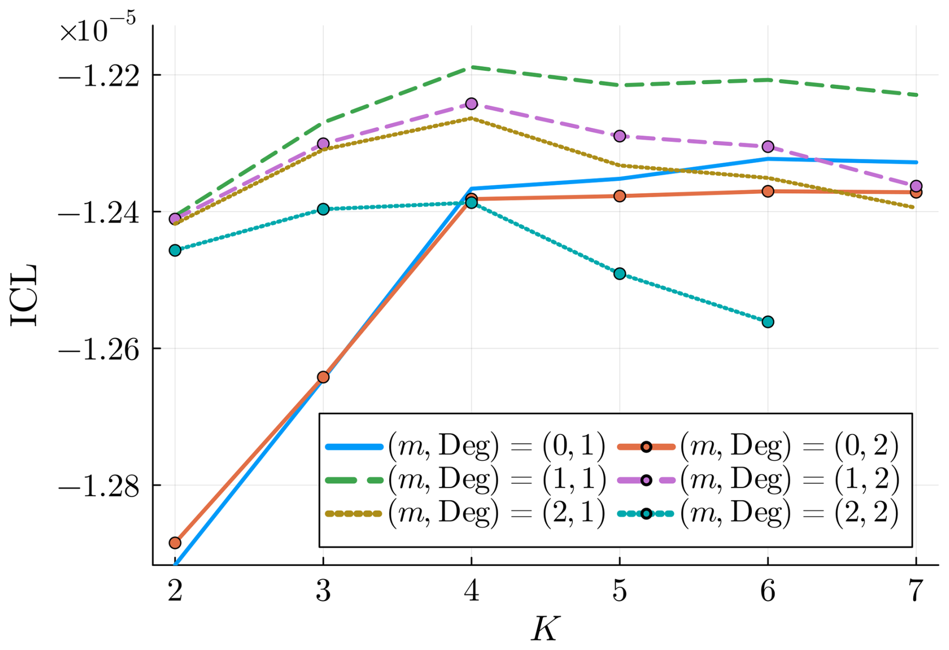
Figure 4 ICL for different values of the hyperparameters. The model with $K=\mathrm{4},m=\mathrm{1}$, and Deg=1 is the maximizer.

3.5 Comparison with multisite WGEN-type models

In this section, we introduce another multisite rain occurrence model that will be used for comparison. This model was first proposed by Wilks (1998) using first-order Markov models to simulate rain occurrence with a Gaussian latent model to generate spatially correlated amounts. Srikanthan and Pegram (2009) later extended it to fourth-order Markov models to better reproduce dry/wet spell distributions. This class of weather generators is also referred to as WGEN-type models (Nguyen et al., 2023) and is typically used alongside rainfall amount models (e.g., Evin et al., 2018). Note that in the literature, the acronym WGEN has also been used to refer to other models. Seasonality is accounted for by assuming that the parameters remain constant within each month.

Mathematically, at each station s∈𝒮 and for a month $\mathrm{mth}\in \left[\right[\mathrm{1}:\mathrm{12}\left]\right]$, rain occurrence follows a Markov model of order m_W, with transition probabilities given by

$$\begin{array}{}\text{(16)}& f_{\mathrm{mth},s}^W(y_s\mid h_s)=\mathbb{P}\left(Y_n^{\left(s\right)}=y\mid H_s^{\left(n\right)}=h_s\right),\end{array}$$

where $H_s^{\left(n\right)}=(Y_s^{(n-\mathrm{1})},Y_s^{(n-\mathrm{2})},\mathrm{\dots },Y_s^{(n-m)})\in {\mathcal{H}}_s^{\left(m_W\right)}:={\mathcal{I}}_s^{m_W}$ is the history variable of order m_W, introduced in Sect. 2.3.

The multisite correlations are modeled using an unobserved Gaussian process U. At each day n∈𝒟 and for a given month $\mathrm{mth}\in \left[\right[\mathrm{1}:\mathrm{12}\left]\right]$,

$$\begin{array}{}\text{(17)}& U^{\left(n\right)}\sim \mathcal{N}(\mathrm{0},{\mathrm{\Omega }}_{\mathrm{mth}}),\end{array}$$

where $U^{\left(n\right)}=\mathit{\{}{U}_s^{\left(n\right)}{\mathit{\}}}_{s\in \mathcal{S}}$, and ${\mathrm{\Omega }}_{\mathrm{mth}}=\mathit{\left\{}{\mathit{\omega }}_{s,s^{\prime }}^{\mathrm{mth}}\mathit{\right\}}$ is an S×S positive-definite correlation matrix.

The rain occurrence $Y_s^{\left(n\right)}$ at site s is determined by the value of $U_s^{\left(n\right)}$. Given a history $h_s^{\left(n\right)}\in {\mathcal{I}}_s^{m_W}$ and the Bernoulli probability $p^W=f_{\mathrm{mth},s}^W(y_s=\mathrm{wet}\mid h_s^{\left(n\right)})$,

$$\begin{array}{}\text{(18)}& Y_n^{\left(s\right)}=\left\{\begin{array}{ll}\mathrm{wet},& \text{if }{U}_s^{\left(n\right)}\le {\mathrm{\Phi }}^{-\mathrm{1}}\left(p^W\right)\\ \mathrm{dry},& \text{otherwise},\end{array}\right.\end{array}$$

where Φ⁻¹ is the quantile function of the standard normal distribution.

As in Srikanthan and Pegram (2009) and Evin et al. (2018), we set the Markov model order to m_W=4. The correlation matrix is estimated following the previous references by simulating each site pair for each month to determine ${\mathit{\omega }}_{s,s^{\prime }}^{\mathrm{mth}}$ that yields the observed correlations, $\mathrm{cor}\left(\mathit{\right\{}{Y}_s^{\left(n\right)}{\mathit{\}}}_{n\in {\mathcal{D}}_{\mathrm{mth}}},\mathit{\left\{}{Y}_{s^{\prime }}^{\left(n\right)}{\mathit{\}}}_{n\in {\mathcal{D}}_{\mathrm{mth}}}\right)$ where 𝒟_mth is the set of all days in month mth.

The model is fitted, yielding ${\mathrm{2}}^{m_W}\times S\times \mathrm{12}$ parameters for the Markov chains and $S(S-\mathrm{1})/\mathrm{2}\times \mathrm{12}$ for the correlation matrices.

The biggest advantage of this model is that it is not limited by the conditional independence hypothesis; i.e., stations can be as close or as far apart as needed. Moreover, the fitting procedure is slightly simpler, as no expectation maximization algorithm is required. The seasonality treatment differs slightly, as WGEN-type models assume parameters to be constant per month, while in our setting, they evolve smoothly throughout the year. Ignoring this minor difference, the complexity of this model is significantly greater than ours. The number of correlation coefficients grows as ∼S², whereas our model scales as ∼K² for the spatial part, with typically K≪S. Thus, while our model is limited in the number of stations due to the conditional independence assumption, WGEN-type models may be constrained in practice by computational complexity. Moreover, as we will show, setting our local history to m=1 provides good results in general, whereas WGEN-type models typically require larger m_W values to adequately reproduce dry/wet sequences (see Sect. 5.2.1). This suggests that part of the temporal dependency is captured by the hidden states, simplifying the local Markov models. Additionally, large-scale dry spells will not be accurately represented, as described in Sect. 5.3. This is not entirely surprising, as WGEN-type models only account for pairwise correlations. Note that higher orders could, in principle, be added at a much greater computational cost.

4 Interpretability: making sense of the hidden states

One of the main messages of this paper is to show that the resulting hidden states are fully interpretable, both spatially and temporally. In particular, forcing conditional independence (see Eqs. 5 and 7) forces all spatial correlations to be in the hidden states.

The discrete latent variable Z∈𝒦 used here corresponds to weather regimes, sometimes referred to as weather types or patterns, which represent a finite set of possible atmospheric states acting as quasi-stationary, persistent, and recurrent large-scale flow patterns. They are commonly used in weather generators to characterize the daily atmospheric circulation (e.g., Garavaglia et al., 2010), which influences the values of the generated variables at the daily timescale. Various methods exist for identifying these weather regimes, with hidden Markov models being one such approach. In our case, these hidden states are not constrained by any external variables and will be interpreted as specialized weather states for France. To our knowledge, no previous approach using spatial HMM has been applied to infer and interpret weather regimes over France (or western Europe). Generally, only a few attempts (e.g., Robertson et al., 2004, Sect. 4) identify and interpret weather regimes without using exogenous variables.

We describe in this section different points of view to give a sense of these hidden states that we also refer to as weather regimes. In the following, all plots and interpretations are done for the model 𝒞_m=1 with K=4 and Deg=1, which was the model selected in Sect. 3.4.

4.1 Spatial features

The hidden states have been introduced to give correlated rain events across France. Hence, we expect the hidden states to form some spatial patterns specific to French weather; typically, the south is generally drier than the north.

4.1.1 Rain probability

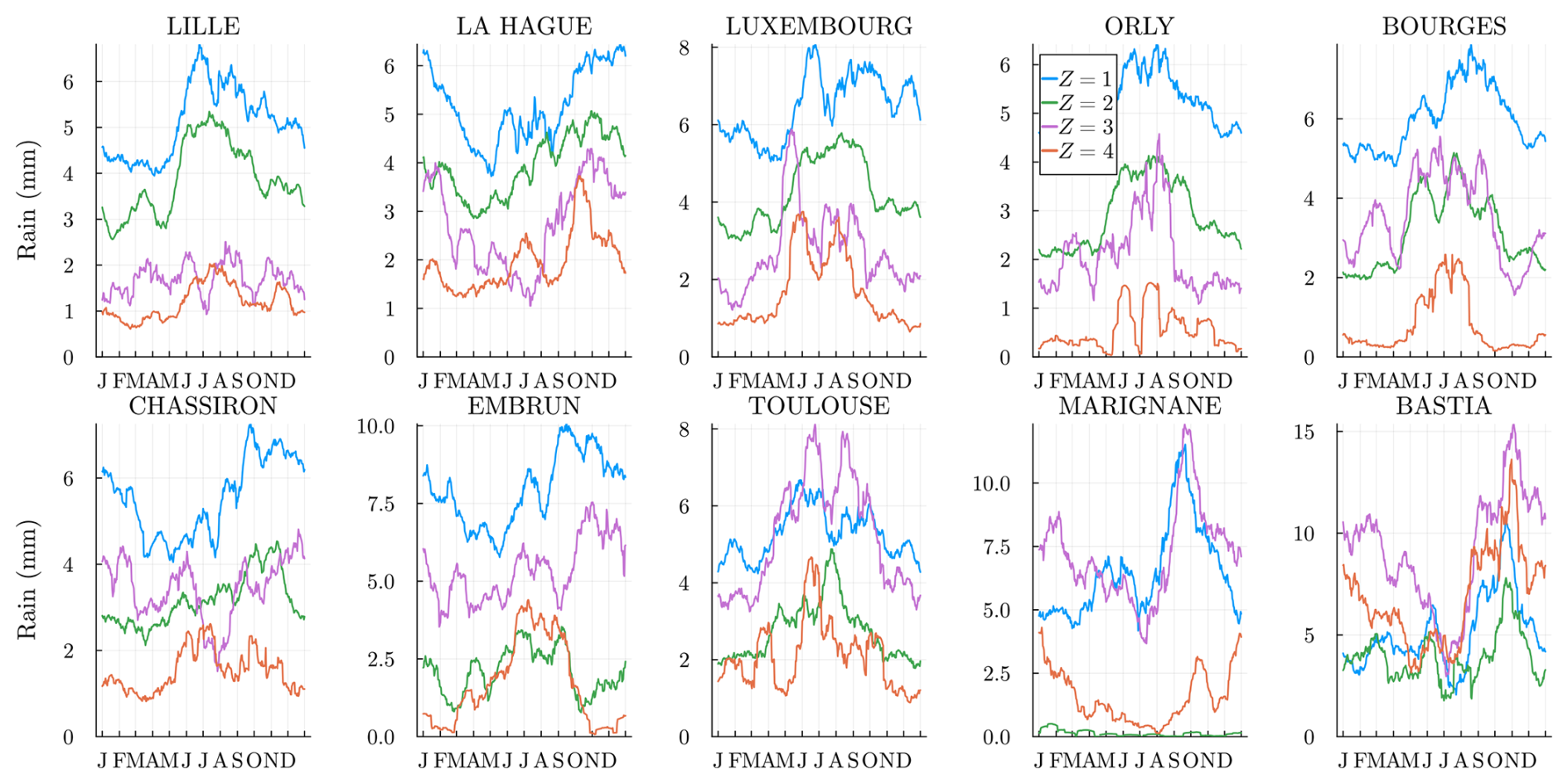
In Fig. 5, we show the rain probability given the hidden state k and that the previous day was dry, averaged over the year. The Z=1 state corresponds to a high probability of rain over all of France, Z=2 corresponds to a rainy climate in the north and drier in the south, and Z=3 is more or less the opposite, while in the state Z=4 the probabilities of rain are low all over France. The trained model satisfactorily recovers known regional features of the French climate. For higher-order models K>4, the spatial features are more and more specific to peculiar regimes, e.g., rainy only in Bastia. It can also be a signal of overfitting.

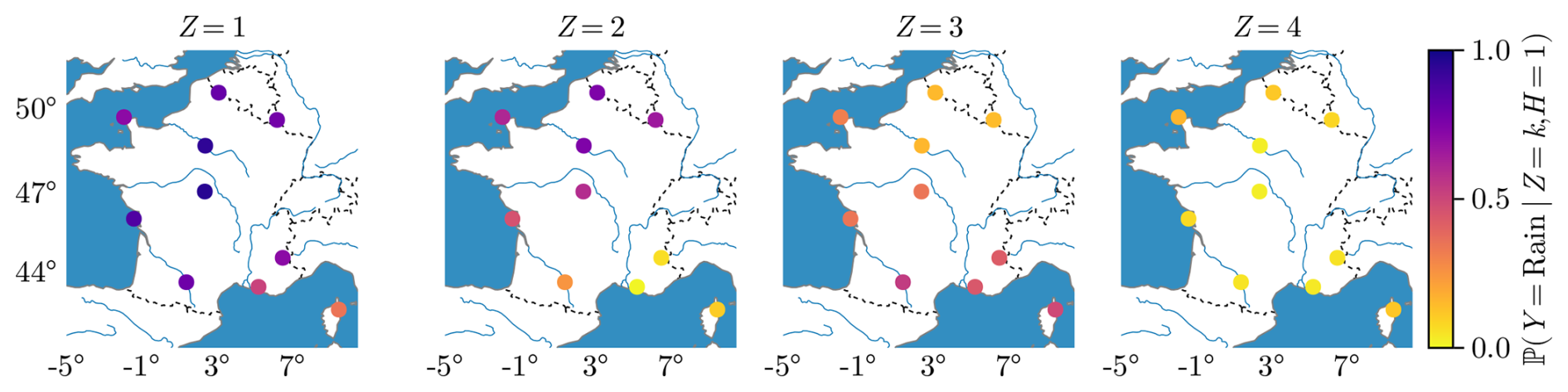
Figure 5 Yearly mean rain probability $T^{-\mathrm{1}}{\sum }_{t\in \mathcal{T}}{\mathit{\lambda }}_{k,t,s,h}$ for m=1 and h=dry, i.e., the probability of rain at a location s, conditional on the hidden state $Z=k\in [\mathrm{1},K=\mathrm{4}]$ and on a previous dry day.

4.1.2 North Atlantic pressure maps

To interpret the model beyond the stations it was trained on and beyond the rain occurrence variable, we will look at the hidden states in terms of weather patterns over the North Atlantic with pressure maps. This is a common practice in climatology and is used to classify weather patterns. For example, the four North Atlantic weather regimes are large-scale weather regimes over the North Atlantic Ocean responsible for most of the climate variability (Woollings et al., 2010). There are various definitions of the regimes of the North Atlantic weather, and it is typically done using clustering methods such as K-means on the daily maps of anomalous 500 hPa geopotential height (e.g., van der Wiel et al., 2019). Note that, as noted in Garavaglia et al. (2010), “it is almost impossible to assert that a given classification is the best” – hence, the comparisons presented in this section are mostly qualitative, as our model classifies weather regimes using only rain occurrence, while other weather variables or classification techniques would yield different regimes.

In Fig. 6, we show how the weather regimes are relevant in terms of pressure maps. We consider the mean sea level pressure (MSP) from the reanalysis ERA5 hourly data on single levels (Hersbach et al., 2020) from 1979 to 2017. The pressure map is averaged over all winter days ${\mathcal{D}}_{\text{W}}=\mathcal{D}\cap \mathit{\{}\text{December},\text{January},\text{February}\mathit{\}}$ conditional on the hidden state (inferred before via the Viterbi algorithm (see Sect. 3.3), giving a pressure anomaly map $\mathrm{\Delta }\text{MSE}={\mathbb{E}}_{t\in {\mathcal{D}}_{\text{W}}}\left(\mathrm{MSP}\left(t\right)\mid {\widehat{z}}_t=k\right)-{\mathbb{E}}_{t\in {\mathcal{D}}_{\text{W}}}\left(\mathrm{MSP}\left(t\right)\right)$ at each longitude and latitude. The geographical area where the pressure maps are computed is $\left(\text{longitude}\in [\mathrm{80}\mathrm{°}\mathrm{W},\mathrm{40}\mathrm{°}\mathrm{E}]\right)$ and $\left(\text{latitude}\in [\mathrm{25}\mathrm{°}\mathrm{N},\mathrm{80}\mathrm{°}\mathrm{N}]\right)$. It is much larger than France and corresponds roughly to the North Atlantic area. The results are shown in Fig. 6.

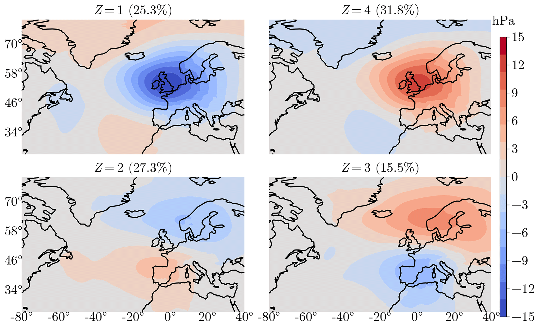
Figure 6 Winter (December–January–February) mean sea level pressure (Pa) anomalies (difference) between the average of all winter days in Z=k state and the average of all winter days. The relative frequency of occurrence of each state during winter in the historical data is shown in parentheses.

The four maps clearly show four distinct regimes with different pressure anomalies. It is remarkable that coherent large-scale structures over mean sea level pressure are found with a model only trained over S=10 stations, all located in France, with rain occurrences as training data.

As a first comparison, we consider the four Euro-Atlantic regimes defined in Cassou (2004, Fig. 7). We display the same differential pressure map as they do over the winter months for a similar spatial domain. In Cassou (2004) and van der Wiel et al. (2019), the four regimes are NAO−, Atlantic Ridge, blocking, and NAO+. The two NAO regimes correspond to the reinforcement or attenuation of the Icelandic low and Azores high, leading to a strengthened or weakened westerly flow over France. The two other regimes correspond to different deviations of this flow, having different consequences for French weather, depending on the season.

In our model selection, we found the same number of hidden states K=4; see Sect. 3.4. If to some extent the states defined by the SHHMM (Fig. 6) look similar to the Euro-Atlantic regimes (see Cassou, 2004, Fig. 7) in terms of the order of magnitude of the mean pressure anomalies (∼10 hPa) and patterns, e.g., Z=4 can be seen as a blocking-like pattern.

However, a close inspection shows important differences: the structures we found are more centered toward France and slightly more intense. This is to be expected as the training data are only in France. A fairer comparison can be found with Boé and Terray (2008), where the weather types (WTs) found with rain amounts in France are also coherent with ours and easier to compare as they represent, like us, the MSP anomalies. They define eight WTs over extended winter months (November to March). WT2 (25 % relative frequency of occurrence) is very close to our Z=4 (31.8 %) in terms of pattern and amplitude, even far outside France. WT6 (12.5 %) is also very close to our Z=3 (15.5 %), i.e., a milder depression centered on the Azores and an anticyclone centered in northern Europe. The other two rainier hidden states Z=1 and Z=2 probably cannot be viewed as simple combinations of the remaining WTs. This is consistent with Boé and Terray (2008), who use rainfall amounts for clustering.

In Garavaglia et al. (2010), the weather patterns (WPs) are found using stations mostly located in the southeast of France and a more complex rain variable. Note that their main figure (Fig. 3) shows the WP geopotential height at 1000hPa averaged all year long, making the comparison with our Fig. 6 harder. Their anticyclonic state (WP8) (25 %) is close to our Z=4, with a pressure high over the north of France and south of Great Britain.

4.2 Seasonality

The SHHMM's transition matrix and distributions have periodic coefficients varying across the year. A consequence is that the hidden states are not fixed in time but can also vary. We expect variations to be smooth enough so that weather regime Z=k has a similar interpretation during the whole year.

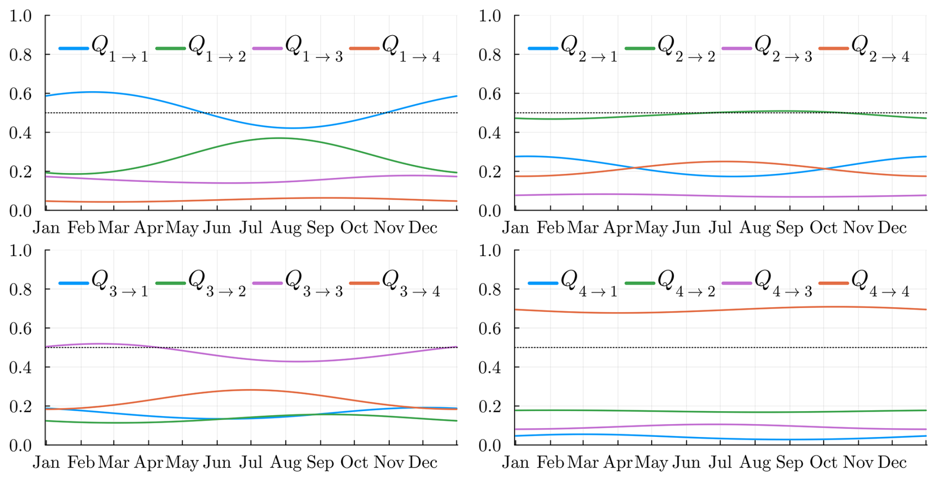
4.2.1 Transition matrix

We display, in Fig. 7, the 16 coefficients of the transition matrix Q_t. The “dry” state Z=4 is the state where the probability of staying in the same state is the highest. Hence, we expect longer global dry sequences than the other regimes. The probability of remaining in the same state is the lowest in states Z=2 and Z=3; hence, these can be seen as transitional states. Moreover, state Z=4 has a very low probability of switching directly to state Z=1 (and vice versa), confirming that an intermediate state is required for this to happen. This makes sense with the intuition that a dry day all over the country is rarely followed by a wet day all over France. During some seasons, e.g., summer (June, July, August, September), state Z=2 will prefer to transition to a dry state Z=4 rather than the wet state Z=1. This is the opposite situation in the rest of the year. Again, this is consistent with the fact that during summer we expect the state Z=1 to be less frequent.

Figure 7 Temporal variation of the transition matrix Q(t) for the SHHMM K=4, Deg=1, and m=1.

4.2.2 Rain probability

We plot, in Fig. 8, the rain probabilities as a function of the station and climate variable Z=k. In almost all stations, the extreme states Z=1 (4) are where it rains most (least) often. As seen in Fig. 5, states Z=2 and 3 are different in the north and south.

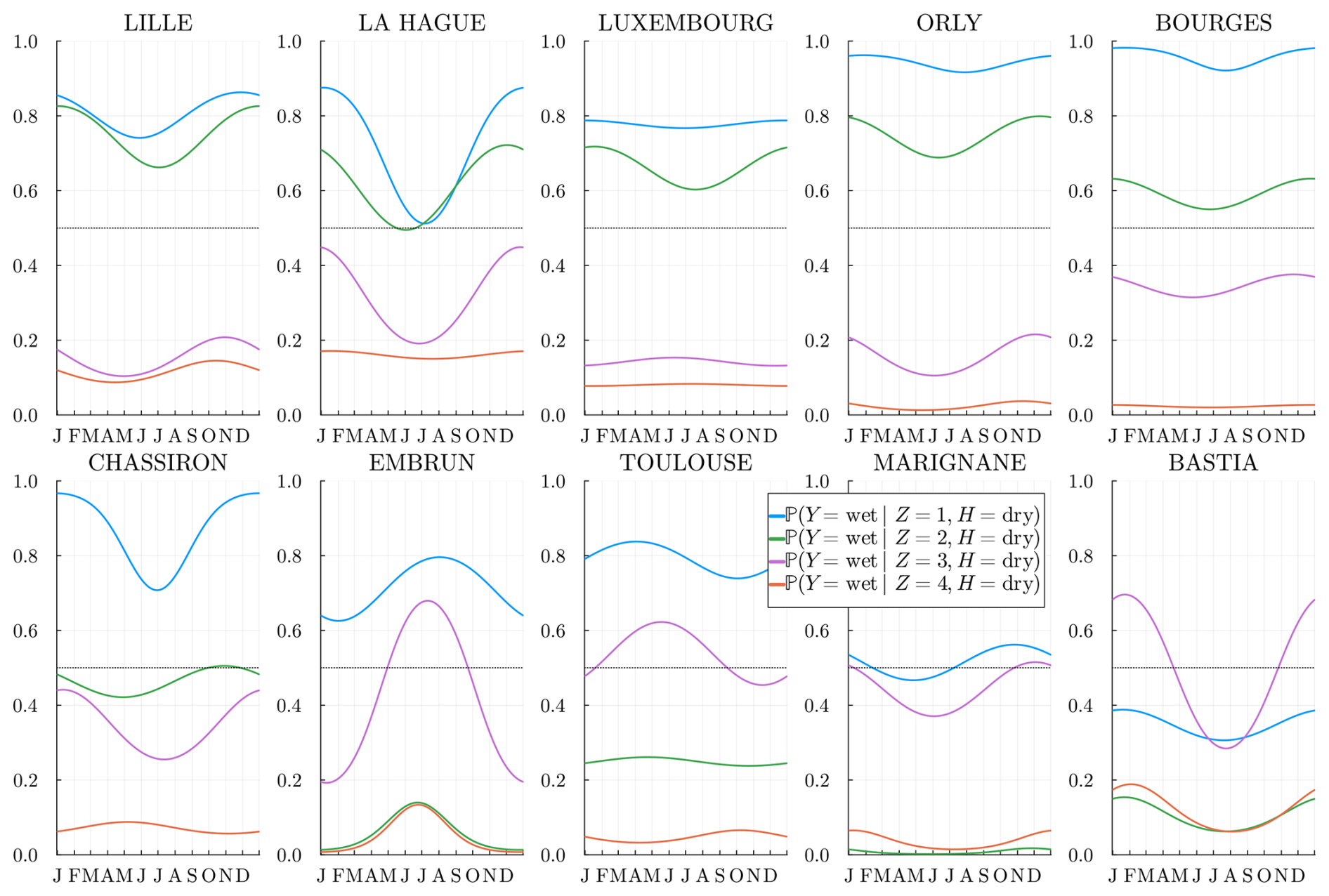
Figure 8 Estimated ${\mathit{\lambda }}_{k,t,s,h}$ probability for m=1 and h=dry, i.e., the probability of rain at the location s, conditional on the hidden state $k\in \left[\right[\mathrm{1},K\left]\right]$ and on a previous dry day. The stations are sorted by latitude from northernmost (top left) to the southernmost (bottom right).

The success of the SHHMM fit can be observed as, at each station, most states are completely separated all year long. That is, in general, the rain probability conditioned on different states Z does not cross states or become equal, showing meaningful states. When converging to local minima, we would typically observe such state crossings during the year, indicating potential issues in the fit.

4.3 Mean rain amount

Even if the model training does not involve any rain amounts $R_s^{\left(n\right)}$, the hidden states Z=k should still be meaningful for these. In Fig. 9, we plot the daily mean rain amount $R_{k,s}^{\left(t\right)}>\mathrm{0}$ for each station and state k. The values obtained are smoothed with a periodic moving average of time window ±15 d; see Appendix D for the definition. The “rainy” weather regime k=1 is the state where it rains the most at almost every location and all year long. Similarly, the “dry” regime k=K is where it rains the least. Interestingly, the intermediate regimes, k=2 and k=3, are rainier in the north in different seasons. Southern stations have a different behavior as expected.

Figure 9 Daily mean strictly positive rain quantity R>0 (mm) at every station per kth component. We smooth the results as in Eq. (D1). We use the model 𝒞₁ with K=4 to get a posteriori the most likely state associated with each date n; see Eq. (F3).

4.4 Weather regime spells

To illustrate the dynamics of the weather regimes, we show in Fig. 10 for different years the Viterbi estimated hidden states $\left(\widehat{z}\right)$ (see Sect. 3.3). As previously noticed, dry and wet spells last longer in general than in other states. For historical events such as the drought in the of summer 1976, we observe a long dry sequence (27 d in a row in state Z=4 starting from 3 June). The famous 2003 heatwave from 1 to 15 August also corresponds to a 15 d dry spell.

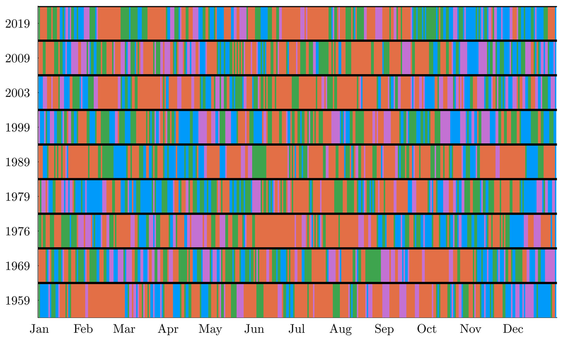
Figure 10 Estimated hidden state sequence for a selection of years. Each color corresponds to a hidden state: Z=1 is blue, Z=2 is green, Z=3 is purple, and Z=4 is orange.

5 Simulations: multisite rain occurrence

Now that the model is fully inferred and interpreted, we will test its validity. To do so, we will sample multiple independent and identically distributed (IID) realizations of the training period 1956 to 2019 and compare several spatiotemporal statistics with the historical data.

5.1 Simulation algorithm of the SHHMM

We first sample the hidden states $(z^{\left(n\right)}:n\in \mathcal{D})$ according to the nonhomogeneous periodic transition matrix ${\mathbf{Q}}_{t_n}$ and initial distribution ξ, and then we draw the MRO $(y^{\left(n\right)}:n\in \mathcal{D})$ from the conditional distributions $f_{z^{\left(n\right)},t_n,s,h_s^{\left(n\right)}}$. The procedure is summarized in Algorithm 2.

Algorithm 2 Simulation of the SHHMM

Result: Sequence hidden states z⁽ⁿ⁾, sequence of MRO y⁽ⁿ⁾

$z^{(n=\mathrm{1})}\sim \mathit{\xi }$

for n∈𝒟 do

$z^{\left(n\right)}\sim {\mathbf{Q}}_{t_n}(z^{(n-\mathrm{1})},\cdot )$

end for

$y^{(n=m-\mathrm{1}:\mathrm{0})}=y_{\mathrm{ini}}^{n=m-\mathrm{1}:\mathrm{0}}$

for n∈𝒟 do

for s∈𝒮 do

$y_s^{\left(n\right)}\sim f_{z^{\left(n\right)},t_n,s,h_s^{\left(n\right)}}(\cdot )$

end for

end for

In the simulations, we choose the initial date as 1 January 1956. Our final date is 31 December 2019 so that the total simulated range is 64 years, which corresponds to our dataset span. We choose $\mathit{\xi }=(\mathrm{1},\mathrm{0},\mathrm{0},\mathrm{0})$, i.e., z⁽¹⁾=1, which is a rainy weather regime, because it was rainy all over France on that day. We assume that the MROs before the first simulation day $y_{\mathrm{ini}}^{n=m-\mathrm{1}:\mathrm{0}}$ are observed and use them as input to draw $y_s^{\left(\mathrm{1}\right)}\sim f_{z^{\left(\mathrm{1}\right)},t,s,h_s^{\left(\mathrm{1}\right)}}$.

The model is lightweight, allowing fast generation – which can easily be parallelized – of many sequences to study climate variability. On a standard computer, generating one 64-year sequence of rain occurrences and hidden states using the StochasticWeatherGenerators.jl package (Métivier, 2024) takes approximately ∼0.01 s.

5.2 Results

In the following, we will use $J=\mathrm{5}\times {\mathrm{10}}^{\mathrm{3}}$ IID. realizations (stochastic simulations) of the SHHMM over a 64-year span and compare its statistics with the 64-year observed sequence and denote by $\mathit{\{}{y}_s^{\left(n\right)}{\mathit{\}}}_{n\in \mathcal{D}}^{\left(j\right)}$ the $j\in \left[\right[\mathrm{1},J\left]\right]$ realizations. When the j is dropped, it refers to the ensemble of all simulations.

5.2.1 Dry/wet state sequence

The dry spell sequences are of particular interest to estimate risks associated with droughts. We show the observed dry (wet) spell distributions, i.e., probability mass function (PMF), in Fig. 11 (and Fig. 12) at all the stations and compare them to the simulated spells for the J realization. When the historical distribution is contained in the simulations' envelope, we may conclude that the model does a good job of reproducing the dry (wet) spells: note that this works systematically well, except for La Hague station (bordering the Channel Sea) at a few data points. In general, for Lille, La Hague, and Chassiron, the observed PMFs deviate from the center of the envelope, suggesting that higher m>1 might be required.

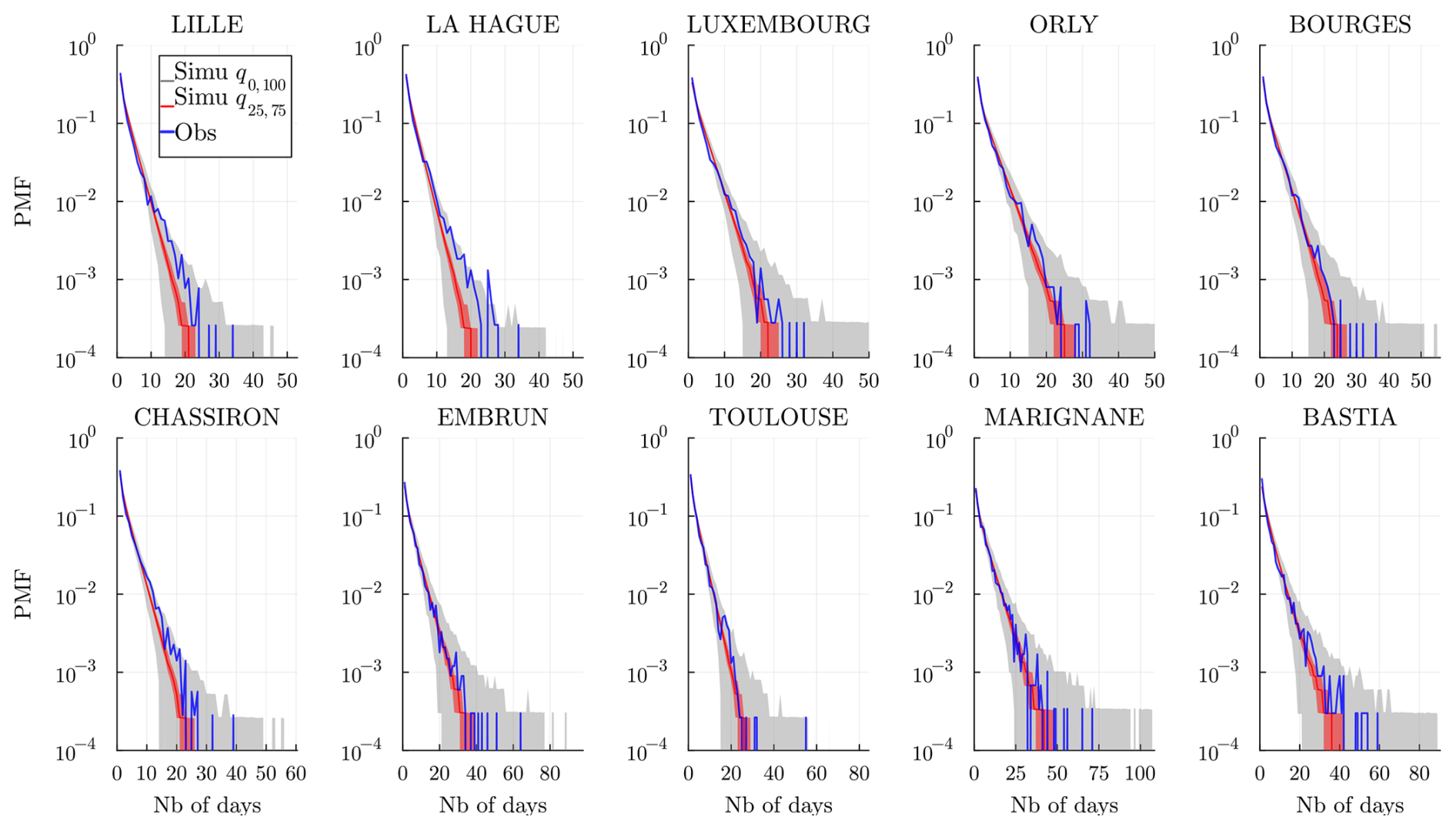
Figure 11 Dry spell distribution (in number of days) at every station and for a time range 𝒟 of the historical data (blue) and of the J=10³ simulated wet spell distribution. The gray envelope covers the full range (q_0,100) of the simulations, while the red envelope covers the interquartile range (q_25,75), and the line (red) is the median. Simulations are obtained over the same time range 𝒟 and using the model $K=\mathrm{4},\mathrm{Deg}=\mathrm{1}$, and 𝒞_m=1.

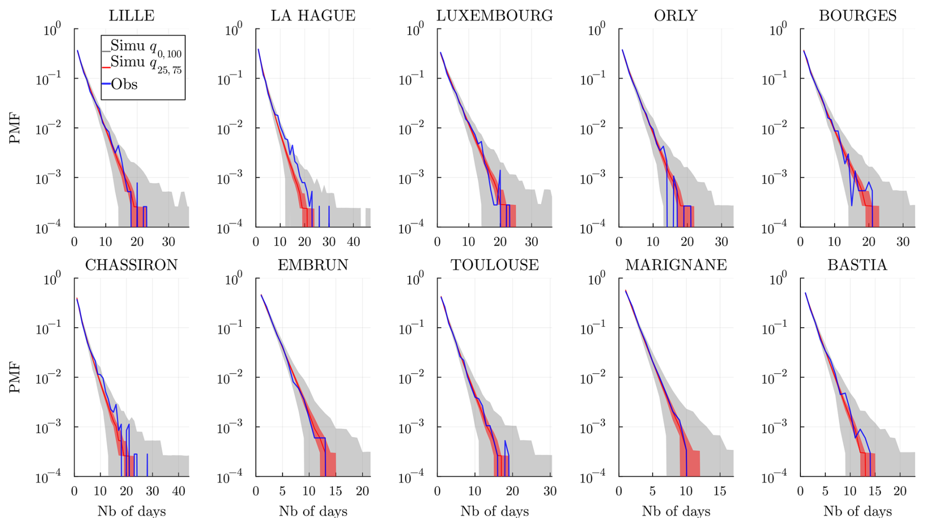
Figure 12 Wet spell distribution (in number of days) at every station and for a time range 𝒟 of the historical data (blue) and of the $J=\mathrm{5}\times {\mathrm{10}}^{\mathrm{3}}$ simulated wet spell distribution. The gray envelope covers the full range (q_0,100) of the simulations, while the red envelope covers the interquartile range (q_25,75), and the line (red) is the median. Simulations are obtained over the same time range 𝒟 and using the model $K=\mathrm{4},\mathrm{Deg}=\mathrm{1}$, and 𝒞_m=1.

In Appendix B, we show and discuss the distribution obtained using the memoryless 𝒞_m=0 model to highlight the gain of the model 𝒞_m=1 in both the center and the tails of spell distributions; see Figs. B1 and B2. We note that even though wet spells are in general much shorter than dry spells, having m=1 is necessary to accurately reproduce the wet spells. Note that the WGEN model presented in Sect. 3.5 is also expected, for a sufficiently high order, to perform well for dry/wet spells, as it is trained at each station to learn the temporal dependence of dry/wet sequences.

5.2.2 Spatial correlations

We compare in Fig. 13 the observed and simulated $S(S-\mathrm{1})/\mathrm{2}$ correlation coefficients between all sites $\mathrm{cor}\left(\mathit{\right\{}{Y}_s^{\left(n\right)}{\mathit{\}}}_{n\in \mathcal{D}},\mathit{\left\{}{Y}_{s^{\prime }}^{\left(n\right)}{\mathit{\}}}_{n\in \mathcal{D}}\right)$ for all $s\ne s^{\prime }\in \mathcal{S}$. Most correlations are well-reproduced, showing that the conditional independence hypothesis in Sect. 2.2 (or Sect. 2.3) is valid.

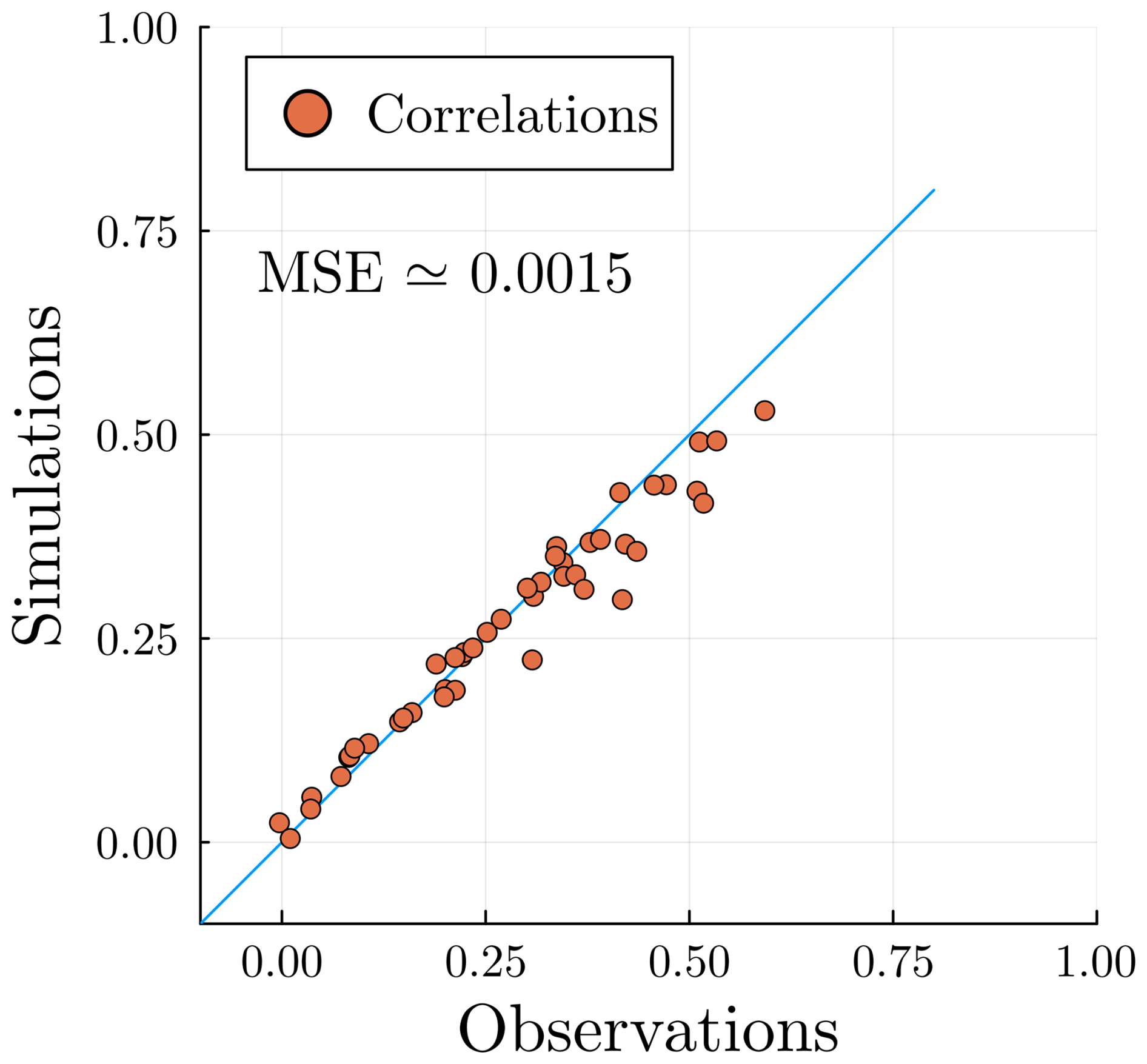
Figure 13 Observed pair correlations $\mathrm{cor}\left(\mathit{\right\{}{Y}_s^{\left(n\right)}{\mathit{\}}}_{n\in \mathcal{D}},\mathit{\left\{}{Y}_{s^{\prime }}^{\left(n\right)}{\mathit{\}}}_{n\in \mathcal{D}}\right)$ for all $s\ne s^{\prime }\in \mathcal{S}$ compared with the correlations computed from the simulations (we average the $J=\mathrm{5}\times {\mathrm{10}}^{\mathrm{3}}$ pair correlations of our simulations). The conditional independence metric MSE_CI in Eq. (19), is displayed in the figure.

To measure this quantitatively, we define the following conditional independence metric:

$$\begin{array}{}\text{(19)}& \begin{array}{rl}{\mathrm{MSE}}_{\mathrm{CI}}& =\sum _{s<s^{\prime }\in \mathcal{S}}\left(\mathrm{cor}\left(\mathit{\right\{}{Y}_s^{\left(n\right)}{\mathit{\}}}_{n\in \mathcal{D}},\mathit{\left\{}{Y}_{s^{\prime }}^{\left(n\right)}{\mathit{\}}}_{n\in \mathcal{D}}\right)\right.\\ & -{\left.{\displaystyle \frac{\mathrm{1}}{J}}\sum _{j=\mathrm{1}}^J\mathrm{cor}\left(\mathit{\right\{}{y}_s^{\left(n\right)}{\mathit{\}}}_{n\in \mathcal{D}}^{\left(j\right)},\mathit{\left\{}{y}_{s^{\prime }}^{\left(n\right)}{\mathit{\}}}_{n\in \mathcal{D}}^{\left(j\right)}\right)\right)}^{\mathrm{2}}.\end{array}\end{array}$$

The closer to zero, the better the conditional independence hypothesis will be satisfied. This criterion helps compare different choices of stations 𝒮; see Sect. 2.1 and Appendix C for more details. This is the biggest limitation of this work: to produce meaningful hidden states that correctly learn spatial correlations, the MSE_CI must be small. For example, a pair of stations at the center of Paris and Orly (only ≃13 km apart) would not satisfy the conditional independence hypothesis. Note, however, that the conditional independence between stations is not necessarily isotropic; hence, station configurations with better MSE_CI are not necessarily those with the largest pairwise station distances.

To give an upper bound to this metric, we trained the model, while keeping seasonality, with K=1 state, i.e., no hidden states (meaning completely independent stations), and found ${\mathrm{MSE}}_{\mathrm{CI}}^{(K=\mathrm{1})}=\mathrm{0.096}$.

5.3 Spatiotemporal spells

To check the spatiotemporal properties of the model, we can focus on the temporal properties of the following spatial quantity: the rain occurrence rate (ROR). Note that a similar quantity is considered in Baxevani and Lennartsson (2015). On a given day n, it is defined as the fraction of stations above some precipitation threshold R_th,

$$\begin{array}{}\text{(20)}& {\mathrm{ROR}}_{R_{\mathrm{th}}}^{\left(n\right)}={\displaystyle \frac{{\sum }_{s\in \mathcal{S}}{\mathbf{1}}_{R_s^{\left(n\right)}>R_{\mathrm{th}}}}{\left|\mathcal{S}\right|}}.\end{array}$$

In general, the precipitation threshold could be made station-dependent, e.g., a given quantile. Such quantities have been used to study large-scale phenomena, e.g., temperature heatwaves (Miloshevich et al., 2023; Cognot et al., 2025). Here, we focus on dry or wet events relevant, for example, for droughts, choosing R_th=0. The previous quantity simplifies to

$$\begin{array}{}\text{(21)}& {\mathrm{ROR}}^{\left(n\right)}={\displaystyle \frac{{\sum }_{s\in \mathcal{S}}{Y}_s^{\left(n\right)}}{\left|\mathcal{S}\right|}}.\end{array}$$

To evaluate large-scale lasting dry events, we consider spells of ROR⁽ⁿ⁾≤0.2; i.e., only 20 % or less of the stations are rainy. We show in Fig. 14 the distribution (PMF) of the spells for each season, i.e., December–January–February (DJF), March–April–May (MAM), June–July–August (JJA), and September–October–November (SON). We observe that the SHHMM is able to reproduce short spells as well as the distribution tails for every season. It can even produce longer spells than observed. On the contrary, the WGEN model overestimates short spell durations while underestimating longer spells. This clearly shows that simple correlation models are not adapted to produce correct large-scale weather events, even though they perform well for pairwise correlation and local dry/wet spells. Using censored Gaussian models, Kleiber et al. (2012) and Serinaldi and Kilsby (2014) consider similar quantities but obtain rather poor results. In contrast, Vaittinada Ayar et al. (2020) achieve good results; however, their model is conditioned on synoptic weather regimes and tested on a much smaller area.

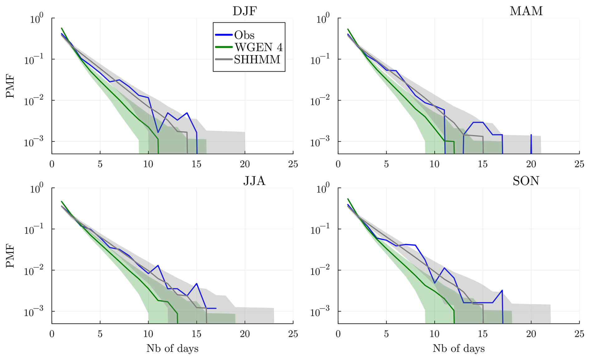
Figure 14 Distribution of spells of ROR⁽ⁿ⁾ lower than or equal to 0.2 for each season. We show in blue the observed spells and in gray the simulations obtained with the SHHMM; in green are the simulations obtained with the WGEN model with Markov chains of order 4. In both cases, the gray envelope shows the quantiles q_5,95 of the $J=\mathrm{5}\times {\mathrm{10}}^{\mathrm{3}}$ simulations, and the line is the median (q₅₀).

6 Modeling: precipitation amount

In this section, we attach to the rain occurrence model 𝒞_m an add-on: a multisite precipitation amount generator. The procedure is carried out hierarchically, i.e., without modifying or retraining the original model. In fact, other variables such as temperature and solar irradiance could be attached similarly to what will be presented in this section. To do so, one only needs a generator for the new variable, e.g., AR(1) model for temperature, and to allow its parameters to depend on the weather regimes Z⁽ⁿ⁾=k and to evolve smoothly (as in Sect. 2.4) with the day of the year t. We hypothesize that the new variable has some dependence on both the weather regime and the season. We discussed in Sect. 4 various spatiotemporal interpretations of the weather regime, and thus it makes sense to consider how this global variable is relevant for other weather variables. Hence, the resulting add-on generator should generate a variable at least partially correlated with the original SHHMM. This makes the model very modular, allowing easy extensions without affecting its original performances and interpretations. Figure 9 highlights the rain amount dependence on the weather regime k and seasonality. This principle is applied in this section to build an add-on rainfall generator.

The multisite rain amount (MRA for short) is denoted R⁽ⁿ⁾ as in Eq. (1). Building an MRA generator directly is hard because of the ambivalent probabilistic nature of rain, being neither a discrete nor a continuous variable. Here we can just focus on strictly positive rain amounts R>0 because the SHHMM directly indicates when R=0 or R>0.

To train the rain amount generator, we will use the hidden states $Z^{\left(n\right)}={\widehat{z}}^{\left(n\right)}$ found in Sect. 3.3. The schematic of the resulting model is shown in Fig. 15.

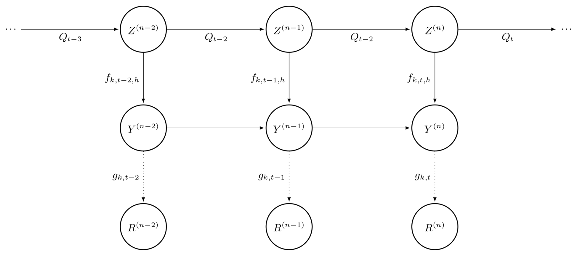
Figure 15 SHHMM with rain amounts. g_k,t denotes the MRA generator with respect to the weather regime k and day of the year t.

6.1 Marginal rain distributions

The rain amount generator we use to fit the marginal distributions R_s>0 at each station is a mixture g(r) of two exponential distributions, with density

$$\begin{array}{}\text{(22)}& g\left(r\right)=w{\displaystyle \frac{e^{-\frac{r}{{\mathit{\vartheta }}_{\mathrm{1}}}}}{{\mathit{\vartheta }}_{\mathrm{1}}}}+(\mathrm{1}-w){\displaystyle \frac{e^{-\frac{r}{{\mathit{\vartheta }}_{\mathrm{2}}}}}{{\mathit{\vartheta }}_{\mathrm{2}}}}.\end{array}$$

This choice is widely adopted in the literature, e.g., Kirshner (2005), Touron (2019b), and Kroiz et al. (2020), and has only three parameters denoted by $\mathit{\gamma }=\mathit{\{}{\mathit{\vartheta }}_{\mathrm{1}},{\mathit{\vartheta }}_{\mathrm{2}},w\mathit{\}}$. It is flexible enough to be used for different climate types and locations. Other popular choices such as gamma (Kroiz et al., 2020; Holsclaw et al., 2016) or heavy-tail distributions (Baxevani and Lennartsson, 2015; Naveau et al., 2016; Tencaliec et al., 2020) could be used at specific locations s or weather regimes k when needed. Note that these heavy-tail rainfall distributions are notoriously hard to estimate (Evin et al., 2016), so we will not consider them in the present paper. See Chen and Brissette (2014) for a review of univariate precipitation models. For example, precipitation in the south of France is less frequent than in the north but more intense, leading to extreme events which are better described with heavy-tailed distributions. In the simulation part, Sect. 7, we show that despite being light-tailed, this choice of generator g(r) trained with respect to weather regimes and seasonality is able to reproduce both the bulk and the tails of most observed rain distributions well.

As in Sect. 2.4, the parameters of the mixture are periodic functions $\mathit{\gamma }\left(t\right)=\mathit{\left\{}{\mathit{\vartheta }}_{\mathrm{1}}\right(t),{\mathit{\vartheta }}_{\mathrm{2}}(t),w(t\left)\mathit{\right\}}$, where ${\mathit{\vartheta }}_{\mathrm{1}\text{or}\mathrm{2}}\left(t\right)=e^{P_{\mathrm{1}\text{or}\mathrm{2}}\left(t\right)}>\mathrm{0}$, $w\left(t\right)=\mathrm{1}/(\mathrm{1}+e^{P_{\mathit{\theta }}\left(t\right)})$ and the P functions are trigonometric polynomials (see Eq. 8).

To fit the mixtures $g_{k,t,s}$ for each station s and hidden state k we use the classical EM algorithm. The maximization step has to be performed with numerical optimization as in Sect. 3. Note that optimization can be done separately for each weather regime k and station s.

6.2 Multisite distribution: Gaussian copula

After training the marginal distributions $g_{k,t,s}$ at each hidden state and site, we now focus on generating correlated multisite rainfall amounts (MRAs). To generate multisite rain occurrences (MROs), we used the conditional independence with respect to the hidden state (and possibly local history). For a vector of Bernoulli (dry/wet) random variables, this was enough to approximate the observed correlation matrix well (see Fig. 13). However, for a vector of non-discrete random variables, such as rain amounts, mixtures of conditionally independent distributions typically underestimate the joint distribution (Holsclaw et al., 2016). It means that despite the hidden states carrying some part of the MRA correlations, we have to add correlations in another way. A classical approach is to use copulas (Nelsen, 2006). Amongst the various families of copula, the Gaussian copula is the easiest to train and manipulate and has been used for weather models (Pandey et al., 2018; Kroiz et al., 2020). In this paper, we will thus train and use a Gaussian copula conditional on the hidden states to generate multisite (strictly) positive rain amounts.

Let $({\mathit{\rho }}_{s,s^{\prime }}{)}_{s,s^{\prime }}$ be the correlations between a pair of stations (s, s^′) for joint rainy events, i.e., $({\mathit{\rho }}_{s,s^{\prime }}{)}_{s,s^{\prime }}=\mathrm{Cor}(R_s|R_s>\mathrm{0},R_{s^{\prime }}|R_{s^{\prime }}>\mathrm{0})$. To reproduce the correct observed (Pearson) correlation $(\mathit{\rho }{)}_{s,s^{\prime }}$, we train a Gaussian copula. A Gaussian copula takes a correlation matrix ${\mathrm{\Sigma }}^{\left(G\right)}=\mathit{\{}{\mathit{\rho }}_{s,s^{\prime }}^{\left(G\right)}{\mathit{\}}}_{s,s^{\prime }\in {\mathcal{S}}^{\mathrm{2}}}$ and the marginal distributions g_s as input. The matrix Σ^(G) is not directly observed, but for an elliptic copula, there is a relationship between the correlation ρ^(G) and the Kendall (rank) correlations (Fang et al., 2002, Theorem 3.1),

$$\begin{array}{}\text{(23)}& {\mathit{\rho }}^{\left(G\right)}=\sin \left({\displaystyle \frac{\mathit{\pi }}{\mathrm{2}}}{\mathit{\rho }}_{\text{Kendall}}\right).\end{array}$$

Hence, to compute ρ^(G), we use the observed Kendall correlation ρ_Kendall , which is preserved under monotonic transformation, such as quantile and cumulative distribution functions (CDFs).

We estimate the correlation matrices ${\mathrm{\Sigma }}_k^{\left(G\right)}=\mathit{\{}{\mathit{\rho }}_{k,s,s^{\prime }}^{\left(G\right)}{\mathit{\}}}_{s,s^{\prime }\in {\mathcal{S}}^{\mathrm{2}}}$ conditional on the hidden state Z=k. Indeed, we expect and observe that the weather regime impacts the correlation. For the driest state Z=K a rain event should be largely independent, and in the rainy state precipitation should be correlated. We actually enforce the conditional independence when k=K; i.e., ${\mathrm{\Sigma }}_K^{\left(G\right)}$ is a diagonal covariance matrix. This choice is also motivated by the lack of observations of joint rain events in the state k=K.

In this work, we also assume, for simplicity, that the correlation matrices have no seasonality dependence, i.e., are independent of the day t. Moreover, we also do not model local temporal correlations for rain amounts. This shortcoming could be overcome using, for example, a spatiotemporal covariance matrix (Benoit et al., 2018).

6.2.1 Simulation procedure

To simulate the rainfall amounts, we first simulate the SHHMM chain $(z^{\left(n\right)},y^{\left(n\right)}:n\in \mathcal{D})$; see Algorithm 2. Then for all the stations where rain is predicted, ${\mathcal{S}}_{\text{wet}}^{\left(n\right)}=\mathit{\{}s:Y_s^{\left(n\right)}=\text{wet},\forall s\in \mathcal{S}\mathit{\}}$, the rain amounts $R_s^{\left(n\right)}>\mathrm{0}$ are generated conditionally using the Gaussian copula with marginal $g_{z^{\left(n\right)},t_n,s}$ and correlation matrix ${\mathrm{\Sigma }}^{\left(n\right)}=\mathit{\{}{\mathit{\rho }}_{z^{\left(n\right)},s,s^{\prime }}{\mathit{\}}}_{s,s^{\prime }\in ({\mathcal{S}}_{\text{wet}}^{\left(n\right)}{)}^{\mathrm{2}}}$.

Remark. In Appendix A, we visually show and with an approximate χ² test that the Gaussian copula model is a valid model for most station pairs. Note that this Gaussian copula can underestimate the joint extreme rain amount (Renard and Lang, 2007), e.g., for close stations. In that case, other copulas might be used, as in Dawkins et al. (2022), for example, but will not be explored in this paper.

7 Simulations: multisite rain amount

In this section, we will test the full multisite model combining the SHHMM and the rain amounts. We will test the marginal distributions, the spatial and temporal correlations, and the seasonality. Note that all previous results of the MRO simulations (see Sect. 5) are still valid since the addition of rain amount is done “on top” of the SHHMM.

In the simulations, we use the parameters obtained in Sect. 3.4: m=1 local memory, K=4 hidden states, and Deg=1 order of trigonometric polynomial. We use the SHHMM transition matrix and Bernoulli distributions obtained in Sect. 3.2 and the rain amount marginal and copula obtained in Sect. 6.

7.1 Correlations

We first compare the spatial correlation of MRA over the 64 years of data; i.e., for all pairs of stations s and s^′ we estimate $\mathrm{Cor}(R_s,R_{s^{\prime }})$. The results are shown in Fig. 16 (left), where observed correlations are compared to simulations. In Fig. 16 (right), we perform a similar comparison for the symmetric tail correlation (or upper tail dependence) (Nelsen, 2006) defined by

$$\begin{array}{}\text{(24)}& {\displaystyle }\begin{array}{rl}\left({\mathit{\rho }}_T{)}_{s,s^{\prime }}\right(q)& =\left(\left({\mathit{\rho }}_T{)}_{s\mid s^{\prime }}\right(q)+({\mathit{\rho }}_T{)}_{s^{\prime }\mid s}\left(q\right)\right)/\mathrm{2}\\ \text{with }\left({\mathit{\rho }}_T{)}_{s\mid s^{\prime }}\right(q)& =\mathbb{P}\left(R>F_{R_s}^{-\mathrm{1}}\left(q\right)\mid R_{s^{\prime }}>F_{R_{s^{\prime }}}^{-\mathrm{1}}\left(q\right)\right)\end{array}\end{array}$$

for $q\in [\mathrm{0},\mathrm{1}]$. The tail correlation indicates how extreme events are correlated at different stations. We observe a good match for most stations; however, for stations with larger tail correlation, ≳0.2, the tail correlation is underestimated by the simulations. This can be an indication that the Gaussian copula is not enough for these pairs of stations. Improvement using the Student copula (whose manipulation is less easy but more capable of generating tail dependence) is a possibility that should be explored in future work.

Figure 16 Comparison of the multisite correlation (a) and symmetric tail correlation in Eq. (24) with q=0.95 (b) from the observed and simulated data. The correlations computed from simulations are averaged over $J=\mathrm{5}\times {\mathrm{10}}^{\mathrm{3}}$ realizations.

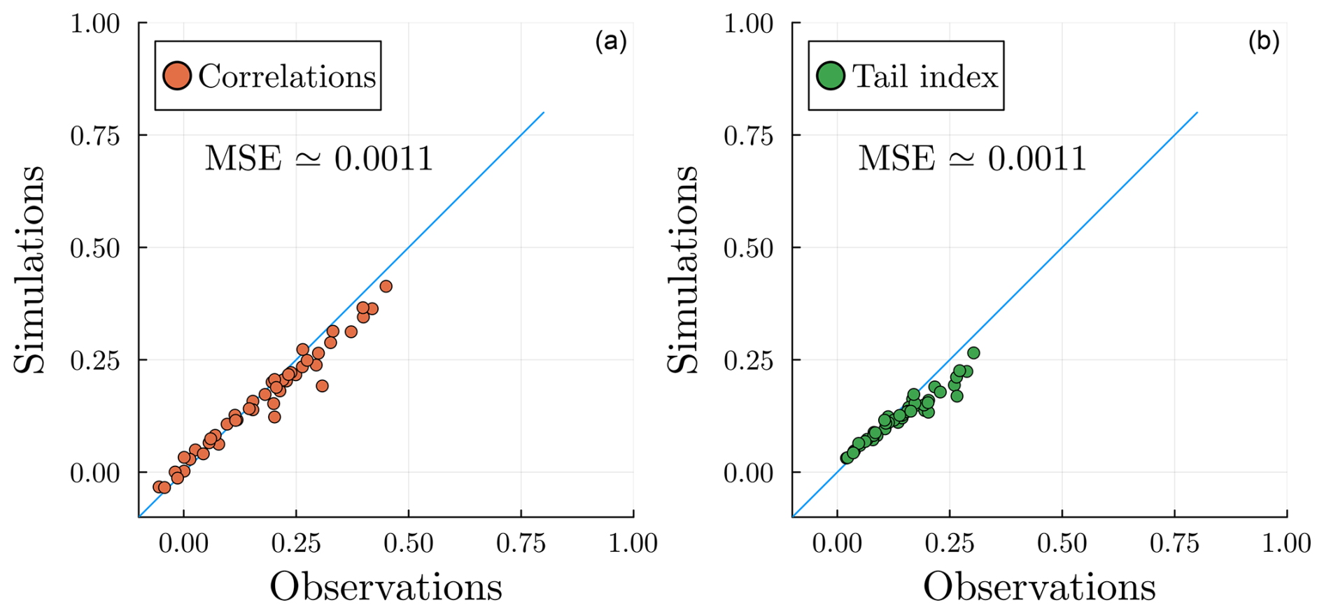
7.2 Rain amounts

7.2.1 Distribution and autocorrelation of precipitation

Figure 17 shows the nonzero rain amount distributions R_s>0 at each station s all year long during the 64-year span of data. It shows the historical distributions (blue) and 5×10³ realizations of our generator (gray). The model reproduces the bulk of the distributions as well as the tails. The observed distribution is in the interquartile range (red envelope) of the simulations up to PDF values $\simeq \mathrm{3}\times {\mathrm{10}}^{-\mathrm{4}}$ for all stations (except for a few points). Even for southernmost stations (Toulouse, Marignane, Bastia) with heavier tails, our model is able to capture most extremes; i.e., the observations lie in the full simulation envelope (gray). This might be due to the seasonal training of the marginals in Eq. (22), allowing the distributions to be more extreme in late summer when heavy storms are common in the south of France. This good performance is interesting in light of recent efforts to use more complex distributions, e.g., generalized Pareto distribution (Naveau et al., 2016; Tencaliec et al., 2020). At some stations like Embrun and Toulouse, it can even generate extremes twice as large as the current maximal value observed, which might be questionable. Note that it cannot reproduce the most extreme rain event at Chassiron (that occurred on 14 August 1972), which in this case shows the limitation of short-tailed exponential distributions.

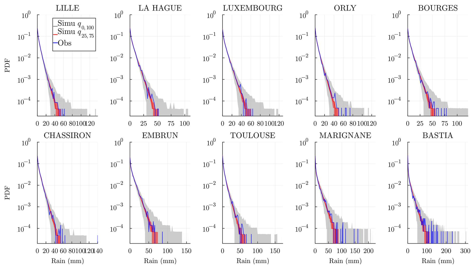
Figure 17 Distribution of the nonzero precipitation amount R>0 (mm) at every station and for all years 𝒯. The distribution of the historical data is shown by the blue line. The gray envelope covers the full range (q_0,100) of the $J=\mathrm{5}\times {\mathrm{10}}^{\mathrm{3}}$ simulations, while the red envelope covers the interquartile range (q_25,75), and the line is the median. To ensure correct representation, the bin intervals of all histograms are set to $\mathrm{0},\mathrm{2},\mathrm{4},\mathrm{\cdots },R_{\max }^{\left(s\right)}\left(\mathrm{mm}\right)$, where $R_{\max }^{\left(s\right)}$ is the maximum rainfall recorded in observations or simulated among the J simulations at the station s.

In Fig. 18, we perform a temporal dependence check for the rainfall amounts (zero and nonzero) by showing the autocorrelation function (ACF) at different lags. The results show that the ACF with lag=1 is always underestimated. This is expected as the current model does not include explicit dependence on the previous day's rainfall, as in Benoit et al. (2018), where the quantity $R^{n+\mathrm{1}}\mid R^n$ is explicitly modeled. The only dependence in our model comes from the weather regimes as well as the autoregressive rain occurrences. Larger lags (>1), however, are better reproduced at most stations. The model fails at La Hague and Chassiron, which are both located on the coast (Channel Sea and Atlantic Ocean, respectively), where the observed dry and wet spells also deviate more from the simulation interquartile range than for other stations.

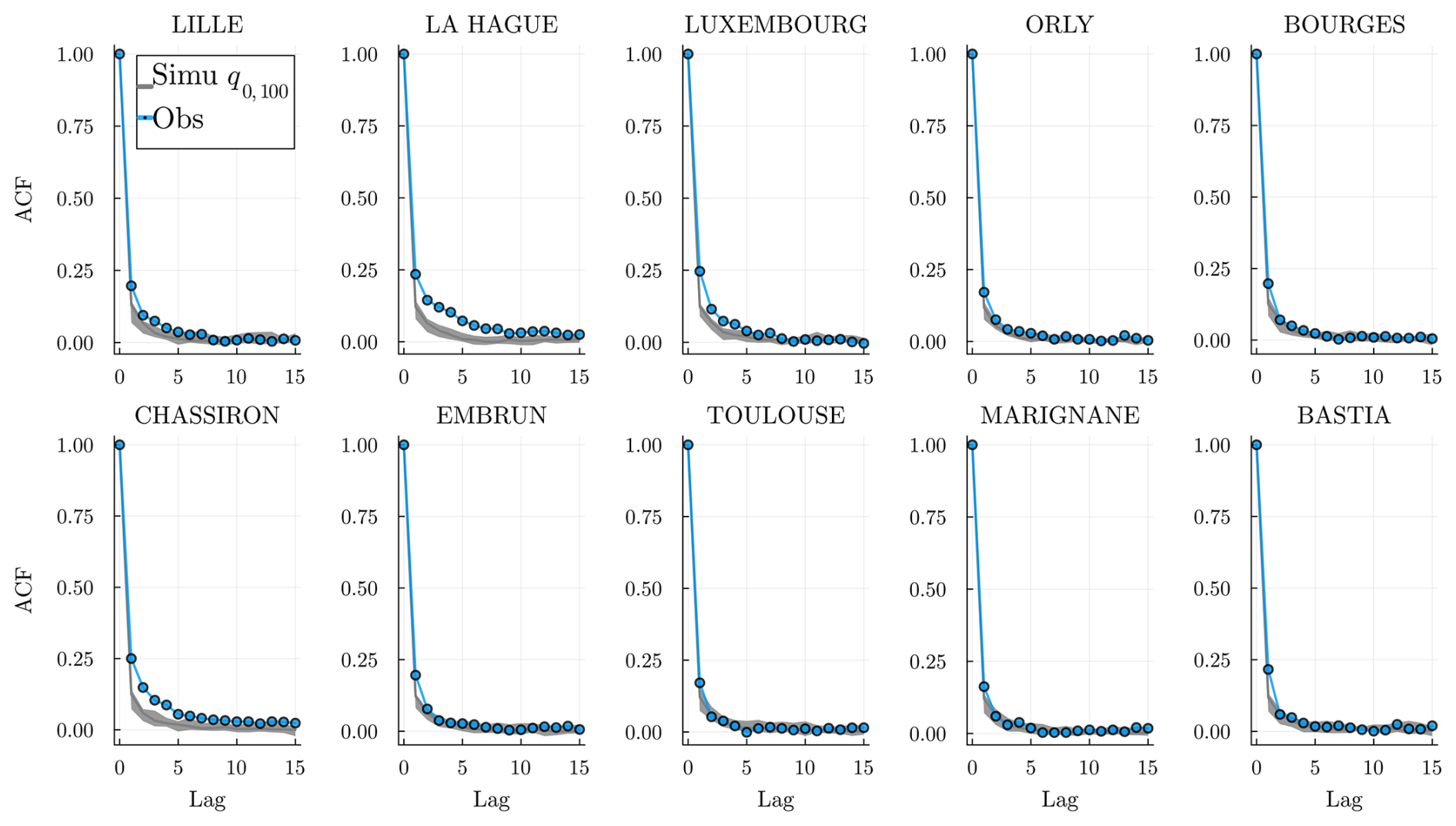
Figure 18 Estimated autocorrelation function (ACF) of the daily rainfall amount R (mm) for lag 0 to 15 at every station and for all years 𝒯. The ACF of the historical data is shown by the blue line. The gray envelope covers the full range (q_0,100) of the $J=\mathrm{5}\times {\mathrm{10}}^{\mathrm{3}}$ simulated ACF.

In the context of flood analysis, a more relevant statistic is the distribution of aggregated rainfall amounts over a period of time. It is crucial, as, for example, heavy rainfall over 5 consecutive days poses a greater risk of flooding than the same amount of rain dispersed over several months. Some models specifically train on these aggregated events (e.g., Evin et al., 2018), while here the only temporal dependence is provided by the underlying HMM. To this end, we display in Fig. 19 the distribution of cumulated rain sequences (non-overlapping) of 5 d. The results again show that the bulk of the distribution (inset) is very well-reproduced, while the tails of the observations generally lie up to 10⁻³ within the interquartile range of the simulations. Once again, the model is able to produce extremes that were not observed, e.g., at Embrun and Bourges. At Chassiron, it fails again to envelope the most extreme observation (which is due to the same extreme event as seen in Fig. 17). The worst results are obtained for La Hague and Chassiron. Again, this is an indication that these two stations require a more complex local model, e.g., higher local memory and dependency on past rainfall amounts.

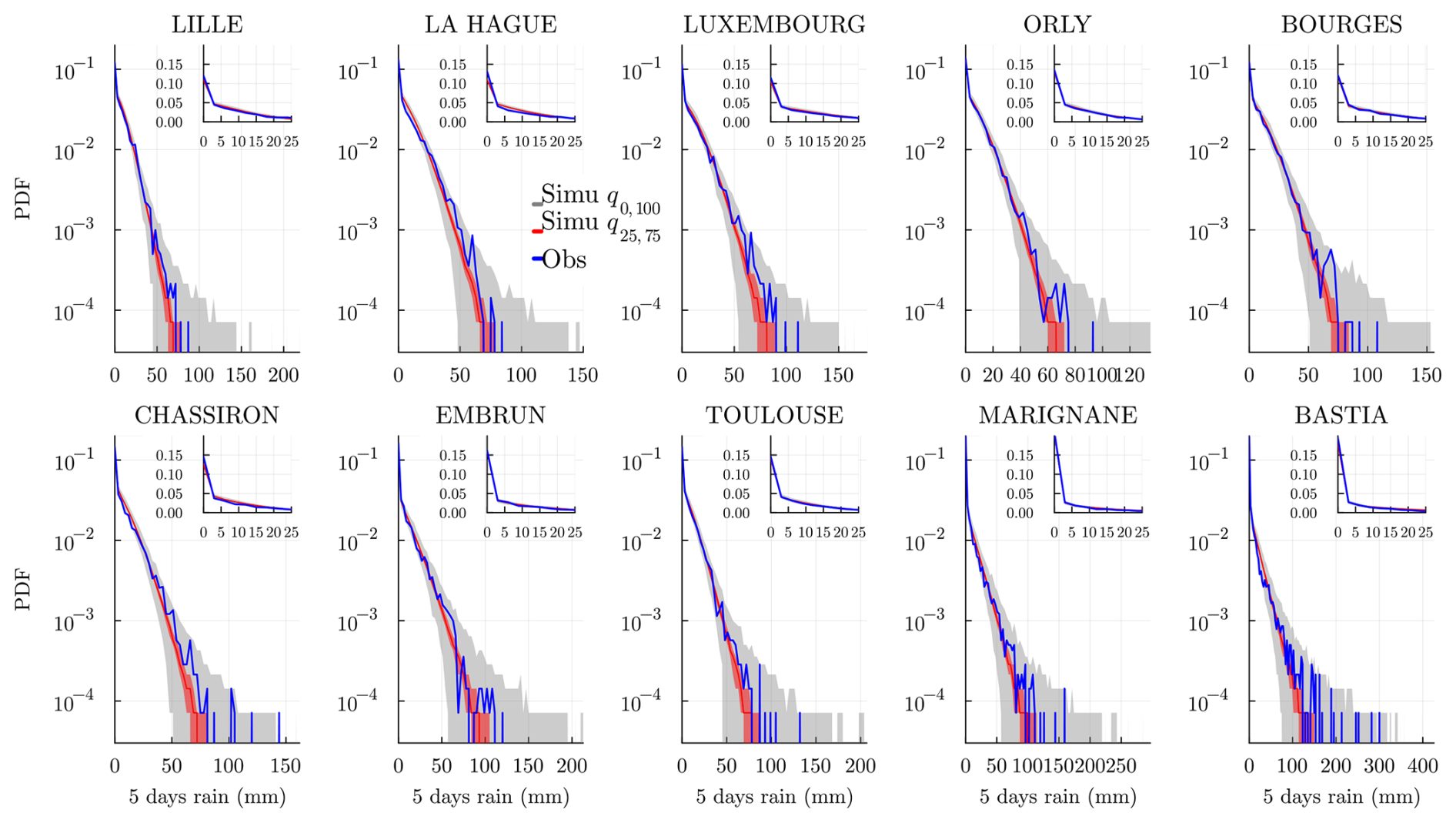
Figure 19 Distribution of cumulated 5 d precipitation amount R (mm) at every station and for all years 𝒯. The distribution of the historical data is shown by the blue line. The gray envelope covers the full range (q_0,100) of the $J=\mathrm{5}\times {\mathrm{10}}^{\mathrm{3}}$ simulations, while the red envelope covers the interquartile range (q_25,75), and the line is the median. In the inset, we show in regular scale a zoom of the bulk of the distribution. To ensure correct representation, the bin intervals of all histograms are set to $\mathrm{0},\mathrm{3},\mathrm{6},\mathrm{\cdots },R_{\max }^{\left(s\right)}\mathrm{mm}$, where $R_{\max }^{\left(s\right)}$ is the maximum of aggregated rainfall recorded in observations or simulated among the J simulations at the station s.

7.2.2 Precipitation during the year

To test the seasonality of the model, we show the quantiles 0.1,0.5, and 0.9 of the accumulated monthly amount at every location. This tests how the model performs in each region and for each month under different regimes (very dry, median, and rainy months). Note that each blue point (historical data) at each station and month is obtained using the observed quantile over 64 points. Hence, it is prone to greater estimation error than most other statistics studied in this paper that use daily observables. Most observed points are located within the envelope of the $J=\mathrm{5}\times {\mathrm{10}}^{\mathrm{3}}$ simulations (colored regions), indicating a fair match with the model. At the southernmost stations, Marignane and Bastia, the observed seasonality does not seem to match that of the model: at the beginning of summer, the model appears to produce rainier July months, while at the beginning of autumn, in October, the generated months are drier than observed. This suggests that the rainfall amount model might not be fully adapted; for example, a higher seasonal dependence (larger Deg) could be required.

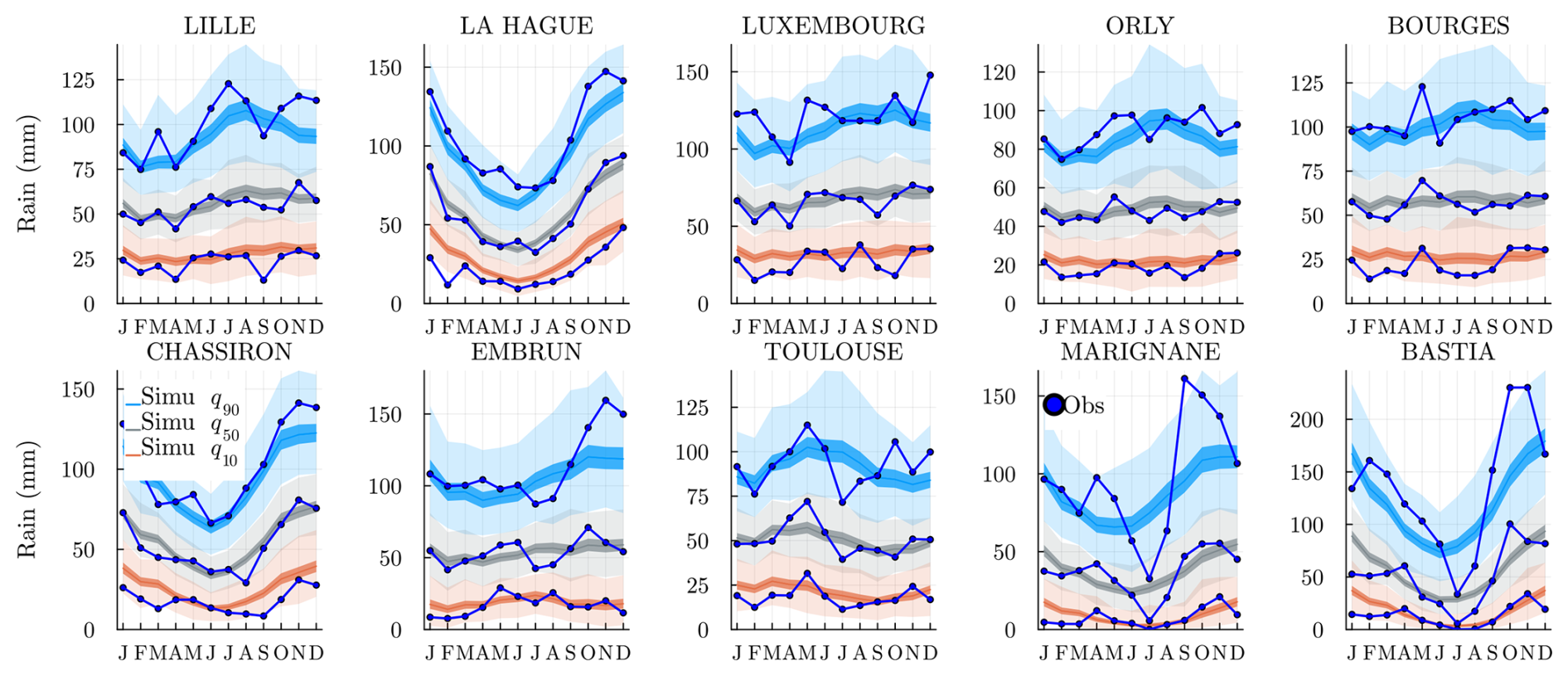
Figure 20 The $(\mathrm{0.1},\mathrm{0.5},\mathrm{0.9})$ quantile of the cumulated monthly mean rain amount in millimeters per month (orange, gray, and light blue, respectively). Historical data (dark blue). For each quantile, we show the envelope of the $J=\mathrm{5}\times {\mathrm{10}}^{\mathrm{3}}$ simulations and in darker colors the [25,75] percentiles, and the line is the median of the simulations.

8 Application to climate change projections

So far, we have trained and validated the SHHMM using historical data. Using the same hyperparameters as found in the model selection (see Sect. 3.4), we can train the model on other datasets. In this section, we show how the stochastic weather generator developed in this paper can be used to study climate change impacts. The focus of the paper is not to perform an in-depth analysis but rather to show, as a proof of concept, how SWG could be useful in that context. To this end, we will train the model with projection data made available by climate model institutes participating in the scientific projects coordinated in the IPCC framework (Arias et al., 2021). A new Coupled Model Intercomparison Project is launched for each new IPCC cycle, and each participating institute runs the latest versions of their global climate model or Earth system model under prescribed radiative forcing conditions. Because these simulations are global and present biases compared to local observations (Tootoonchi et al., 2023), we will use the downscaled and bias-adjusted projections provided by the French climate service DRIAS. It is based on a selection of regional projections made in the international CORDEX initiative based on CMIP5 global projections (projections made in the framework of the 5th IPCC assessment report).

8.1 DRIAS data

We use the DRIAS website (Soubeyroux et al., 2021) that aggregates different regional (European) projections forced by some chosen global projections made by different institutes. DRIAS-2020 provides 30 climate projections (2006–2100) with three scenarios (RCP2.6, RCP4.5, and RCP8.5) and 12 historical simulations (1951–2005). These simulations are further downscaled and bias-adjusted over France using the ADAMONT method (Verfaillie et al., 2017) with SAFRAN reanalysis (Vidal et al., 2010) covering France with 8 km resolution for many daily variables. We select the closest grid points to the S=10 considered stations and extract the precipitation amount. The exact grid point choice should not matter too much, since the reanalyzed simulations are smoothly interpolated. Since these physical models tend to overestimate the frequency of light rain amounts R, we set to R=0 all amounts smaller than 0.1 mm to match what is done at the experimental weather stations.

8.2 Direct comparison of models with the reference period

Climate models provide historical simulations (1951–2005) to be able to validate models against observed data. Because a model does not simulate the same interannual variability as observed, the evaluations are based on the statistical properties of the variables rather than on their chronology. For example, in Fig. 21, we compare the monthly rain quantiles computed as in Sect. 7.2 obtained from the historical climate simulations and from the SHHMM simulations (the same as previously trained on historical observation). We use here two climate models, Aladin (CNRM-ALADIN63 – CNRM-CERFACS-CNRM-CM5) and IPSL (IPSL-WRF381P – IPSL-IPSL-CM5A-MR), as an example. Using an SWG allows a better sampling of the natural climate variability because it is possible to run many more realizations than can be done with climate models. This sample can then be used to check how climate model simulations are positioned. For example, at Lille station, in July for the 0.9 quantile, we observe that the historical point around ≃120 mm (blue) is far from the two climate models (orange and green): ≃100 mm. However, when looking at the predicted statistical envelope, the climate models are exactly at the median, while the historical observation is actually an extreme value. When comparing the two climate models, we observe that the IPSL model produces more points outside the statistical envelope than the Aladin model, suggesting that the model may present stronger biases.

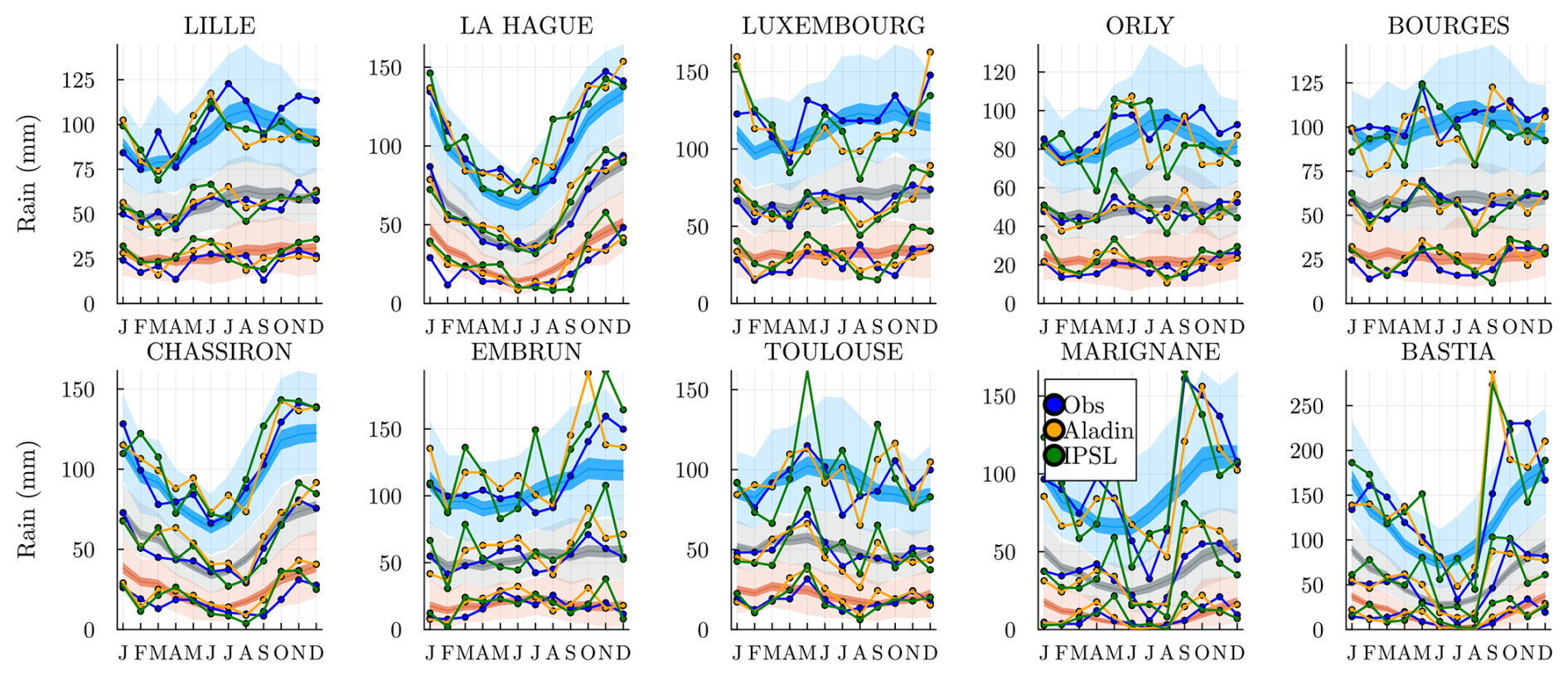
Figure 21 Same as Fig. 20 with added monthly rain quantile for the model Aladin (CNRM-ALADIN63 – CNRM-CERFACS-CNRM-CM5) and IPCC (IPSL-WRF381P – IPSL-IPSL-CM5A-MR) for the reference period 1952 to 2006.

We can perform the same comparison task on dry spell distributions with the Aladin model; see Fig. 22. Again, the SWG samples allow for comparison of the climate model within the predicted variability. At a lot of stations, e.g., Marignane, Orly, and Toulouse, the results are within the interquartile range. However, we can also observe that in the tails, the climate model is always under or equal to the historical curve. This raises the question of whether climate models are able to produce yet unseen extremes.

Figure 22 Same as Fig. 11 with the dry spell distribution of Aladin (CNRM-ALADIN63 – CNRM-CERFACS-CNRM-CM5) for the reference period 1952 to 2006.

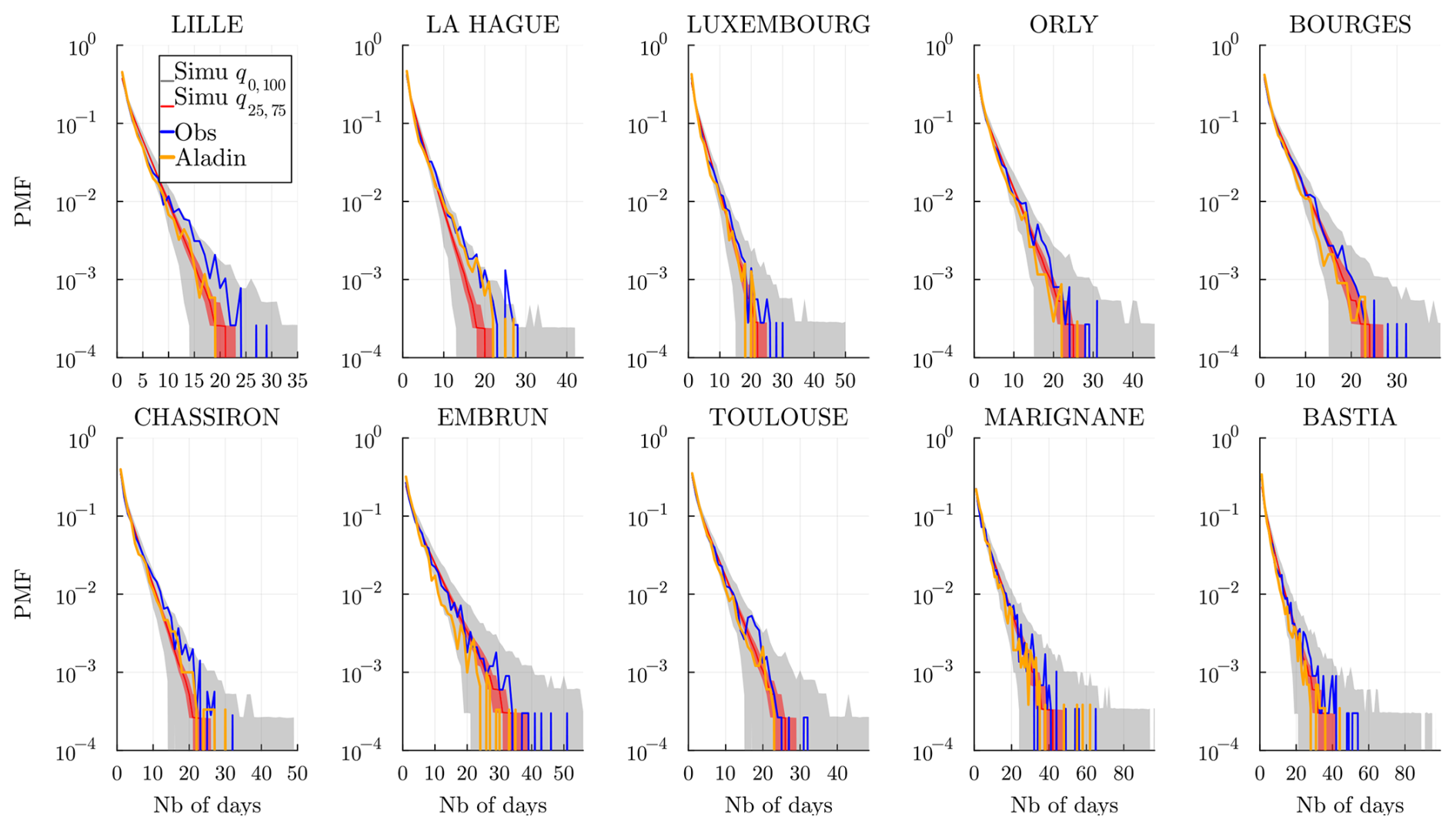
8.3 Training on RCP scenarios

Once the comparison has been made for the historical period, in this section, we will study how the spatial rainfall may evolve in the future by fitting the SHHMM on climate model projections under different RCP scenarios. The RCP scenarios are designed to represent differentiated trajectories of greenhouse gas and aerosol emissions that drive climate change until the end of the century (and beyond in some cases). To do so, we select the data over a 64-year range, here 2032–2096, which simplifies the statistical comparison with the 64-year range of the historical data we considered.

In Fig. 23, the transition matrices obtained when training on historical and IPSL-RCP8.5 data are compared. The aim here is only to highlight the ability of the SHHMM to be used in climate change conditions, not to conduct an impact study; that is why only one climate model is used. The two matrices are still close, meaning that the hidden states of our model are robust to parameter evolutions. However, we can observe interesting differences. For example, Q_3→3 and Q_1→1 are significantly larger in summer months. The weather regimes 1 and 3 were interpreted as rainy all over France and heavy rain in the south, respectively. This means that the IPSL model under RCP8.5 projects longer stretches of heavy rain. Figure 24 shows the analog of Fig. 20 with simulations from the trained SHHMM with IPSL-RCP8.5 data and in blue the historical data. It clearly shows that the IPSL model under the RCP8.5 scenario projects rainier periods. In fact, it is known that the regional climate model for the EURO-Coordinated Regional Downscaling Experiment used in all DRIAS models presents this type of bias (Boé et al., 2020; Vautard et al., 2021). In particular, summer periods are consistently rainier, even for the 0.1 quantile of the monthly mean rain amount. This example shows how the proposed SWG can be used to analyze and compare models: either directly interpreting the coefficients change or sampling from the fitted model to study extreme behaviors.

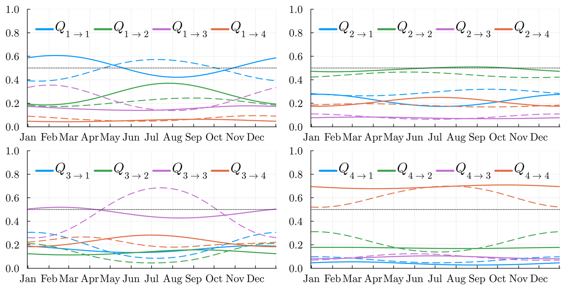
Figure 23 Temporal variation of the transition matrix Q_t trained on historical data (plain line) and on RCP8p5 from IPSL-WRF381P data (dashed line) for the period 2032–2096.

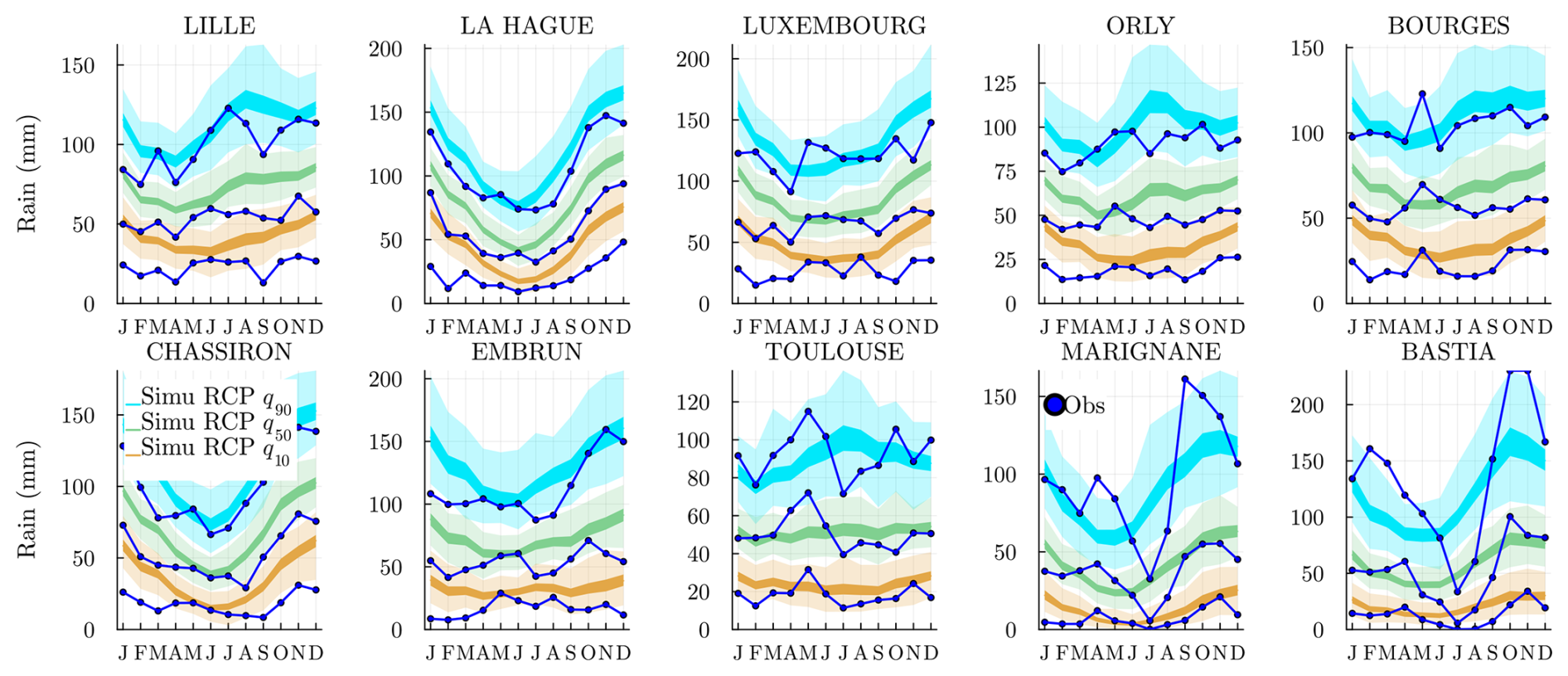
Figure 24 The $(\mathrm{0.1},\mathrm{0.5},\mathrm{0.9})$ quantile of the cumulated monthly mean rain amount in millimeters per month (orange, green, and light blue, respectively). Historical data (dark blue) and J=10³ realization of the model trained with the RCP8p5-IPSL-WRF381P data for the period 2032–2096. For each quantile, we show the envelope of the J simulations and in darker colors the [25,75] percentiles and the median. Note that the color palette has been slightly modified with respect to Fig. 20 to highlight that these envelopes are obtained with simulations from the model trained on an RCP scenario.

9 Conclusions

In this paper, we define a multisite stochastic weather generator for precipitation named the seasonal hierarchical hidden Markov model (SHHMM). Even though it is based on a hidden Markov model introduced for weather applications in the 1990s, we propose an original combination of features based on two important assumptions: (a) the conditional independence for the multivariate rain occurrence (MRO) variable (see Eqs. 5–7) and (b) the imposed smooth seasonal evolution of most model parameters (see Sect. 2.4). Assumption (a) forces the model to learn spatial correlations, leading to fully interpretable hidden states (weather regimes). This differs from part of the literature, where hidden states and correlation coefficients are trained jointly with continuous variables or additionally conditioned on predefined synoptic-scale variables. Thanks to the discrete nature of MRO and the station locations, we checked the validity of hypothesis (a); see Fig. 13. Assumption (b) is natural and has been introduced before in Touron (2019a); it stabilizes training, i.e., removes a lot of identifiability issues that occur while training nonhomogeneous HMMs, and leverages the relatively small number of observation years. To capture more of the local weather, i.e., station-wise, we introduced an autoregressive dependence of rain occurrence on past weather, allowing better temporal correlations.

The model inference and identifiability were analyzed. In particular, we proposed an efficient heuristic initialization in Sect. 3.1 to accelerate model training during the Baum–Welch expectation maximization algorithm and additionally demonstrated that the model must satisfy specific identifiability conditions to remain meaningful in Sect. 2.5. To the best of our knowledge, these aspects have not been previously discussed in the literature. The model selection was performed using the integrated complete-data likelihood criteria, leading in particular to the selection of four hidden states extensively interpreted as France-wide weather regimes in Sect. 4. In particular, we were able to showcase how the hidden states found can be compared to several Euro-Atlantic and France-centered weather regimes defined in other works. These hidden states were shown to be robust to different choices of stations; see Appendix C. The model was extensively tested with simulations. Its performance in reproducing dry and wet spells, as well as the amount of precipitation, is very good, even in the tails of the distributions at most stations. Our model was compared with WGEN, a widely used model in the literature, and was found to better reproduce the distribution of areal dry spells.

The model's hierarchical structure allows for easily adding other weather variables on top of the HMM without modifying the hidden states. In fact, new variables, such as rainfall amount, benefit from the trained hidden states and can be adjusted conditionally on them. The rainfall amount was also tested in terms of distribution, autocorrelation, 5 d aggregated distribution, monthly aggregated quantile, and spatial correlation, with good performance.

Eventually, we showed how this generator can be used with climate change models. One can evaluate climate models on the reference period by comparing them to the estimated climate variability obtained with many simulations of the SWG, as in Figs. 21 and 22. This approach can give more relevant results than only comparing the climate models to a single historical observation. Additionally, training the SWG model on future climate projections allows for interpreting changes across all model parameters (see Fig. 23) or resampling from these future scenarios to better estimate variability and extremes; see Fig. 24.

The major limitation of the model is the assumption (a) that forces careful choice of the stations, as noted already in Zucchini and Guttorp (1991). Even though we show in Appendix C that the precise station choice does not significantly affect the hidden states as long as the MRE_CI is low, finding a valid station set can be a hard problem. This first model lays the groundwork for a fully seasonal spatiotemporal SWG working on a large scale with no external exogenous variables.

Having inferred the weather regime only from rain occurrences and not amounts might also not be completely satisfying, as other clustering methods using rainfall amounts or geopotential have found more complex patterns, particularly for extreme rain. Rain occurrences might limit the number of meaningful patterns, as Robertson et al. (2004) also found four hidden states using a spatial HMM for northeast Brazil, which has a completely different climate. To circumvent these limitations, one could try to train a spatial HMM with rain amounts and/or more complex variables. However, we caution against such complexities, as they can tend to produce hidden states very dependent on the chosen imperfect parametric distribution; see Pohle et al. (2017) and de Chaumaray et al. (2023). Another solution, keeping only rain occurrences, could be to break conditional independence to allow many more stations in the region of interest, which would be able to discriminate between more complex patterns. It was explored partially in Hughes and Guttorp (1994b) and Kirshner et al. (2004) by allowing pairwise correlations or tree structures with the hidden states. Keeping interpretable hidden states while breaking conditional independence is a challenge left for future research.

Many smaller improvements could also be considered, such as different models for rain amount or seasonality at different locations to account for regional specificities. A temporal correlation with previous rain amounts is also possible with a spatiotemporal correlation matrix (Benoit et al., 2018; Bennett et al., 2018) to improve the precipitation autocorrelation function (ACF). Another question is how to incorporate nonstationarity in the model's hidden states, such as climate change trends. So far, these have been added using the generalized linear model framework with exogenous variable dependence on the parameters (e.g., Greene et al., 2011, or Dawkins et al., 2022).

Extending the model with new weather variables, such as temperature on top of the current model (and its hidden states), is another challenging problem that can be addressed with this model. Indeed, the weather regimes identified here are likely relevant for other weather variables such as temperature, solar radiation, and wind. They could therefore be used to train conditional models for these additional variables (hierarchical dependence). In fact, this idea was tested by training an SWG on five daily weather variables (rainfall amount, minimum and maximum temperature, solar irradiance, and evapotranspiration) using the same hidden states identified in this paper. The simulation outputs were then coupled with a crop model to produce a hackathon dataset; see Métivier et al. (2025) and references therein. Note that this is ongoing work. In a similar spirit, another option to include more densely packed stations could be to couple the SHHMM and its pre-trained large-scale weather regimes with a local high-resolution model. In this case, the hidden states would serve as exogenous variables. However, compared to other models where these inputs are fixed over a training period, our hidden states are modeled specifically for the large-scale area of interest and can be regenerated as needed to explore climate variability over the period of interest, e.g., with future climate scenario data.

Adding new weather variables and higher-resolution models at specific locations to extend the SHHMM could be useful in many large-scale risk analysis studies. For example, river water (temperature and flow) used to cool power plants can be modeled based on the weather (typically temperature and rainfall) over the relevant catchment areas (e.g., Nguyen et al., 2023). With an extended SHHMM, one could assess the resilience of the entire French nuclear power plant fleet under climate change projections, e.g., by estimating the probability of having half of the plant generation simultaneously limited due to long-lasting, large-scale droughts. Exploring this extension is left for future work.

Appendix A: Gaussian copula

To check the Gaussian copula approximation for the joint rain events between station pairs, we transform our data into an empirical bivariate distribution with normal margins to test its quantiles against those of a true bivariate normal distribution. Note that these checks are mostly qualitative since we apply the procedure to time series, meaning we are outside the IID framework where these kinds of tests are valid.

In detail, given a pair of stations $(s,s^{\prime })$ and a hidden state Z=k, we consider the joint positive rain amount $R_{s,s^{\prime },k}=(R_s>\mathrm{0},R_{s^{\prime }}>\mathrm{0})\mid Z=k$ for all dates n, so we can remove the superscript n. We first have to transform the observations to pseudo-observations, i.e., $R_{s,s^{\prime },k}\in {\mathbb{R}}_{+}^{\mathrm{2}}\stackrel{\mathit{\eta }}{⟶}(u_{s,k},u_{s^{\prime },k})\in [\mathrm{0},\mathrm{1}{]}^{\mathrm{2}}$. There are several possible transformations η, e.g., the estimated marginal CDF or ordinal ranking. We use the latter one as done in the package Copulas.jl (Laverny and Jimenez, 2024) that we use for all our copula simulations. These pseudo-observations are then transformed to normal distributions using the transformation $X_{s,s^{\prime },k}=\left({\mathit{\varphi }}^{-\mathrm{1}}\right(u_{s,k}),{\mathit{\varphi }}^{-\mathrm{1}}(u_{s^{\prime },k}\left)\right)$, where ϕ⁻¹ is the quantile function of the standard normal distribution. For a vector x∈ℝⁿ and an n×n correlation matrix Σ_M, the squared Mahalanobis distance is defined as

$$\begin{array}{}\text{(A1)}& D_{\mathrm{M}}\left(x\right)=x^{⊺}{\mathrm{\Sigma }}_{\mathrm{M}}^{-\mathrm{1}}x.\end{array}$$

We use the correlation coefficients ${\mathit{\rho }}_{s,s^{\prime },k}^{\left(G\right)}$ obtained in Sect. 6.2 to build the 2×2 matrix Σ_M and compute the Mahalanobis distance for all samples. For a true bivariate normal distribution, the distribution of D_M follows a χ²(ν) distribution with ν=2 degrees of freedom. In Fig. A1, we compare the quantile of the χ²(ν=2) distribution with the $D_{\mathrm{M}}\left(X_{s,s^{\prime },k}\right)$ for two pairs of stations and each hidden state Z=k. Note that we simplify the analysis, considering only one covariance matrix instead of the four fitted in Sect. 6.2. The correspondence is good even for close pairs. It means that Gaussian copulas are adapted when stations are far enough apart. For Z=1, i.e., the rainiest weather, only 3 out of 45 station pairs fail the one-sided Kolmogorov–Smirnov test with the 95 % confidence level that compares the theoretical χ²(ν=2) distribution with the observed squared Mahalanobis distance. These are the pairs Bourges–Orly, Lille–Orly, and Lille–Luxembourg, which are amongst the closest pairs; see, e.g., Fig. A1 (left). Interestingly, for a slightly bigger distance, the pair (334 km) Orly–La Hague passes the test; see Fig. A1 (middle). This indicates anisotropy in the correlation repartition. For other weather regimes Z>1, the Gaussian copula hypothesis also works well for most stations with enough data.

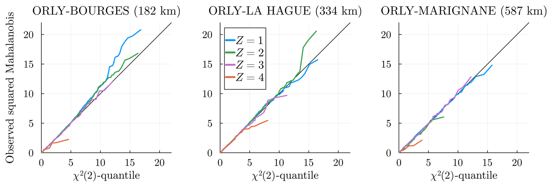
Figure A1 Three examples of q–q plots to test the Gaussian copula hypothesis. The squared Mahalanobis distances between station pairs vs. χ²(ν=2) distribution are shown. A good match means that the Gaussian copula hypothesis to generate pairs $(R_s>\mathrm{0},R_{s^{\prime }}>\mathrm{0})\mid Z=k$ is satisfied.

Appendix B: Comparison with the memoryless model 𝒞_m=0

In Sect. 2.2 and 2.3 we define and model 𝒞_m=0 and 𝒞_m>0. We later selected 𝒞_m=1 using the ICL criteria; see Fig. 4. We show here the performance of the 𝒞_m=0 model in terms of dry/wet spells in Figs. B1 and B2. The observed distribution is shown, while the $J=\mathrm{5}\times {\mathrm{10}}^{\mathrm{3}}$ simulation quantile envelopes are displayed. These figures are to be compared with Figs. 11 and 12 produced by the 𝒞_m=1 model. In the bulk of the spell distributions, i.e., short spells with higher probability, the difference is important (note that the log scale tends to visually minimize the effect), e.g., Embrun and Marignane for the dry spells and all wet spell distributions. This indicates that the model 𝒞_m=0 without local memory overestimates very short wet spells (and dry spells to a lesser degree). At some stations, it also underestimates the longer spells (tails), e.g., Bastia for wet spells.

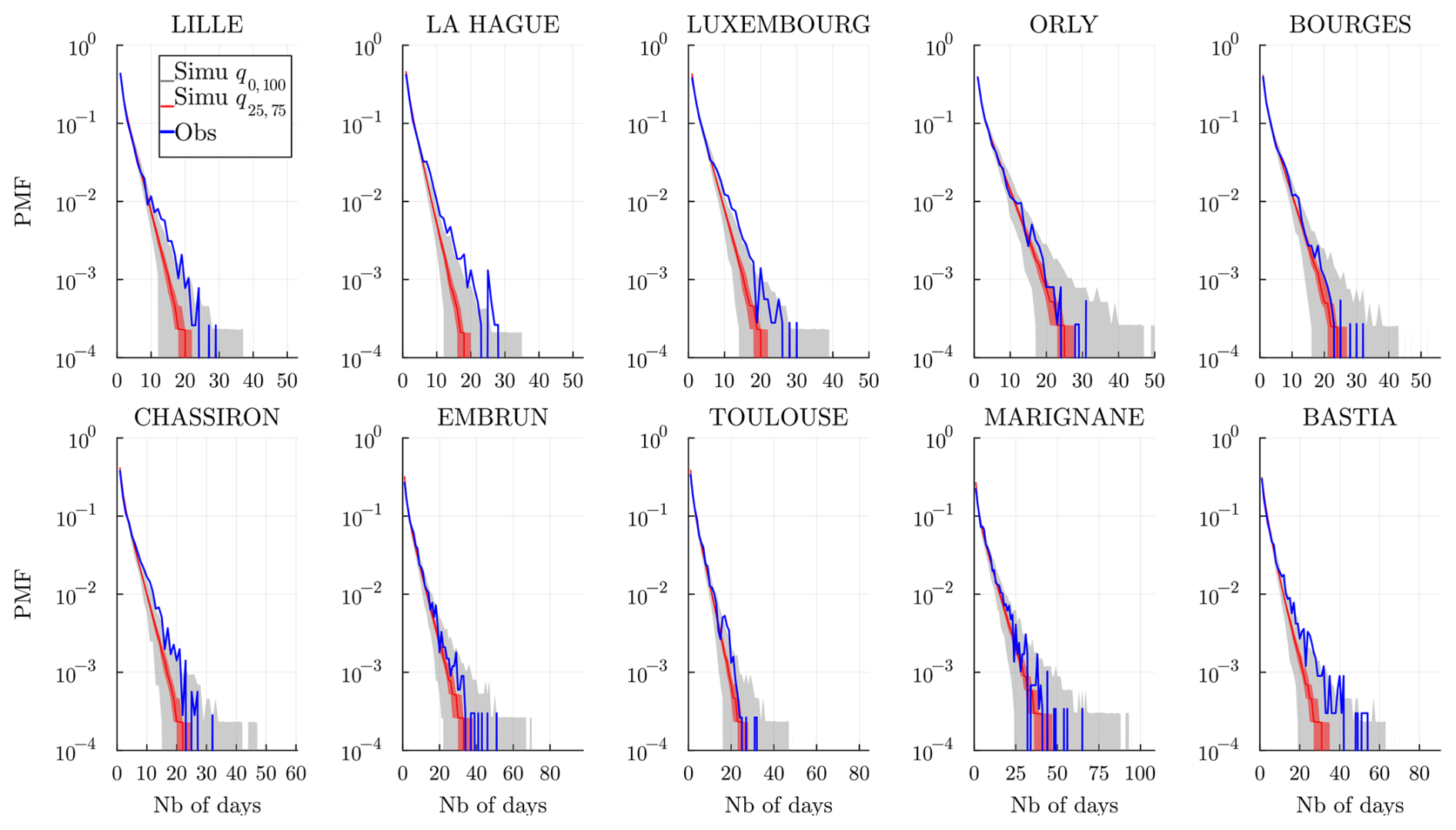
Figure B1 Dry spell distribution (in number of days) at every station and for a time range 𝒟 of the historical data (blue) and the $J=\mathrm{5}\times {\mathrm{10}}^{\mathrm{3}}$ simulated wet spell distribution. The gray envelope covers the full range (q_0,100) of the simulations, while the red envelope covers the interquartile range (q_25,75), and the line is the median. Simulations are obtained over the same time range 𝒟 and using the memoryless model $K=\mathrm{4},\mathrm{Deg}=\mathrm{1}$, and 𝒞_m=0.

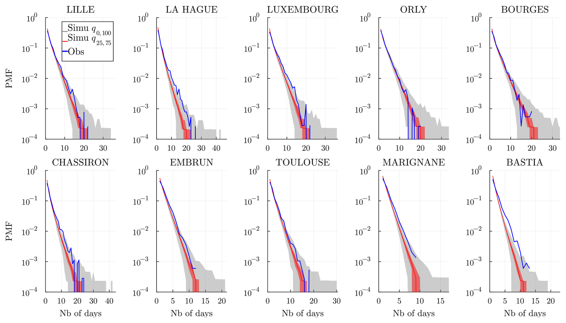
Figure B2 Wet spell distribution (in number of days) at every station and for a time range 𝒟 of the historical data (blue) and the $J=\mathrm{5}\times {\mathrm{10}}^{\mathrm{3}}$ simulated wet spell distribution. The gray envelope covers the full range (q_0,100) of the simulations, while the red envelope covers the interquartile range (q_25,75), and the line is the median. Simulations are obtained over the same time range 𝒟 and using the memoryless model $K=\mathrm{4},\mathrm{Deg}=\mathrm{1}$, and 𝒞_m=0.

Appendix C: Comparison with other station choices

In this Appendix, we show that the hidden states, i.e., weather regimes, found in the main text with our choice of stations 𝒮 (see Sect .2.1) are robust to station changes. We replaced all stations with their closest station within a ≤150 km radius. In cases where no neighbor was found, the station was kept. With our pool of 66 stations and the original set, we replaced 8 out of 10 stations. The resulting moved station set, 𝒮_moved, is given in Table C1. Note that the Luxembourg_A station is different from the Luxembourg station (at the airport) used in the paper.

We trained our SHHMM with the stations in 𝒮_moved using the same procedure as before. The resulting transition matrix is shown in Fig. C1. The new transition matrix (dotted line) is almost identical to the original one (full line) found in Sect. 4.2.1. The mean probabilities conditional on the hidden states of 𝒮_moved (crosses) are also very close to those of 𝒮 (circles), exhibiting the same spatial pattern; see Fig. C2.

Table C1 Original station set 𝒮 and set 𝒮_moved with the closest available station within a 150 km radius. In bold are the stations we kept for which no neighboring station was available in the given radius.

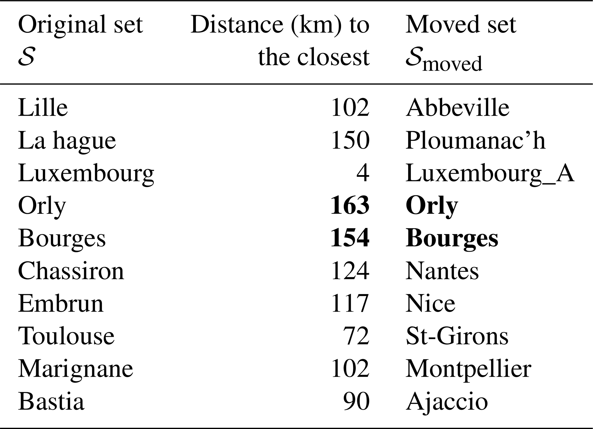
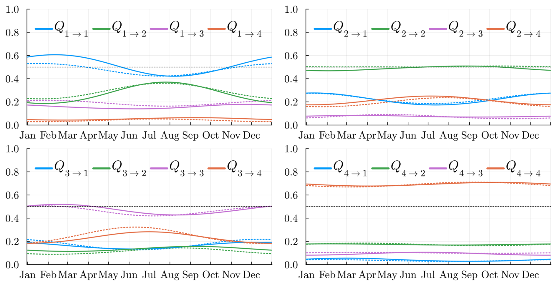
Figure C1 Temporal variation of the transition matrix Q(t) for the SHHMM K=4, Deg=1, and m=1. The full line is the matrix trained on the original set 𝒮, and dotted lines correspond to the model trained on the set 𝒮_moved.

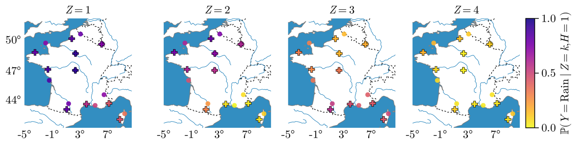
Figure C2 Yearly mean rain probability $T^{-\mathrm{1}}{\sum }_{t\in \mathcal{T}}{\mathit{\lambda }}_{k,t,s,h}$ for m=1 and h=dry, i.e., the probability of rain at a location s, conditional on the hidden state $Z=k\in [\mathrm{1},K=\mathrm{4}]$ and on a previous dry day. The circle represents the results obtained when training with the 𝒮 set, while the cross indicates the result when training with the 𝒮_moved set. Bourges and Orly appear in both sets, causing the circle and cross to overlap. Additionally, Luxembourg and Luxembourg_A are nearly positioned on top of each other.

Appendix D: Periodic moving average

We define the periodic moving average used in Fig. 9. Given a T-periodic observable X^(t) for t∈𝒯, the associated moving average ${\overline{X}}^{\left(t\right)}$ is given by

$$\begin{array}{}\text{(D1)}& {\displaystyle }{\overline{X}}^{\left(t\right)}=\sum _{h=-H}^{h=H}\mathcal{K}\left({\displaystyle \frac{h}{H}}\right){\displaystyle \frac{X^{(t+h)}}{{\sum }_{h=-H}^{h=H}\mathcal{K}\left({\displaystyle \frac{h}{H}}\right)}},\end{array}$$

where $t\in \left[\right[\mathrm{1},T\left]\right]$, $X^{(t\pm T)}=X^{\left(t\right)}$, and 𝒦 is a kernel. In the paper, we choose the window size H=15 with the Epanenchikov kernel $\mathcal{K}\left(u\right)=\frac{\mathrm{3}}{\mathrm{4}}(\mathrm{1}-u{)}^{\mathrm{2}}{\mathbf{1}}_{\left|u\right|\le \mathrm{1}}$ and T=366.

Appendix E: Baum–Welch algorithm for seasonal hierarchical HMM

We use the same model 𝒞_m>0 as described in Sect. 2 and will describe the inference procedure using the Baum–Welch algorithm for a seasonal hierarchical HMM (SHHMM).

We recall that θ stands for all the SHHMM $(\mathit{\xi },{\mathbf{Q}}_{\mathrm{t}},f_{k,t,h}{)}_{k\in \mathcal{K},t\in \mathcal{T},h\in {\mathcal{H}}^{\left(m\right)}}$ parameters (see Sect. 2.3). To fit the model, we must find the θ maximizing the observed likelihood,

$$\begin{array}{}\text{(E1)}& {\displaystyle }\begin{array}{rl}{\mathcal{L}}_{\mathit{\theta }}& \left(y^{(\mathrm{1}:N)}\right)={\mathbb{P}}_{\mathit{\theta }}\left(Y^{(\mathrm{1}:N)}=y^{(\mathrm{1}:N)}\right)\\ & =\sum _{z^{\left(\mathrm{1}\right)},\mathrm{\dots },z^{\left(n\right)}}{\mathbb{P}}_{\mathit{\theta }}\left(Y^{(\mathrm{1}:N)}=y^{(\mathrm{1}:N)},Z^{(\mathrm{1}:N)}=z^{(\mathrm{1}:N)}\right)\\ & =\sum _{z^{\left(\mathrm{1}\right)},\mathrm{\dots },z^{\left(n\right)}}{\mathcal{L}}_{\mathit{\theta }}\left(y^{(\mathrm{1}:N)},z^{(\mathrm{1}:N)}\right)\\ & =\sum _{z^{\left(\mathrm{1}\right)},\mathrm{\dots },z^{\left(n\right)}}{f}_{z_N,t_N}\left(y^{\left(N\right)}\mid h^{\left(N\right)}\right)\\ & {\mathbb{P}}_{\mathit{\theta }}\left(Y^{(\mathrm{1}:N-\mathrm{1})}=y^{(\mathrm{1}:N-\mathrm{1})},Z^{(\mathrm{1}:N)}=z^{(\mathrm{1}:N)}\right)\\ & =\sum _{z^{\left(\mathrm{1}\right)},\mathrm{\dots },z^{\left(n\right)}}{f}_{z_N,t_N}\left(y^{\left(N\right)}\mid h^{\left(N\right)}\right)Q_{z^{(N-\mathrm{1})},z_N}\left(t_N\right)\\ & \mathbb{P}\left(Y_{\mathrm{1}:N-\mathrm{1}},Z^{(\mathrm{1}:N-\mathrm{1})}=z^{(\mathrm{1}:N-\mathrm{1})}\right)\\ & =\sum _{z^{\left(\mathrm{1}\right)},\mathrm{\dots },z^{\left(N\right)}}{\mathit{\xi }}_{z^{\left(\mathrm{1}\right)},h_{\mathrm{1}}}{f}_{z^{\left(\mathrm{1}\right)},t_{\mathrm{1}}}\left(y^{\left(\mathrm{1}\right)}\mid h^{\left(\mathrm{1}\right)}\right)\\ & \prod _{n=\mathrm{2}}^N{Q}_{z^{(n-\mathrm{1})},z_n}\left(t_n\right)f_{z_n,t_n}\left(y^{\left(n\right)}\mid h^{\left(n\right)}\right),\end{array}\end{array}$$

where the index $z_n\in \left[\right[\mathrm{1},K\left]\right]$ for all n∈𝒟 values.

The Baum–Welch algorithm is an iterative expectation maximization, where the likelihood is increased sequentially, i.e., at each step (i) of the algorithm ${\mathcal{L}}_{{\mathit{\theta }}^{\left(i\right)}}\le {\mathcal{L}}_{{\mathit{\theta }}^{(i+\mathrm{1})}}$.

Let us detail the procedure and show that the classical element of the Baum–Welch algorithm for an HMM (homogeneous) proof remains valid when considering an SHHMM. The first step is to consider the conditional expectation of the log-likelihood of the parameter θ, ℒ_θ, with respect to the parameter at step (i), θ⁽ⁱ⁾,

$$\begin{array}{}\text{(E2)}& {\displaystyle }\begin{array}{rl}\mathcal{R}\left(\mathit{\theta },{\mathit{\theta }}^{\left(i\right)}\right)& ={\mathbb{E}}^{{\mathit{\theta }}^{\left(i\right)}}\left[\log \mathcal{L}\left(Y^{(\mathrm{1}:N)},Z^{(\mathrm{1}:N)};\mathit{\theta }\right)\mid Y^{(\mathrm{1}:N)}\right]\\ & =\sum _{k,l=\mathrm{1}}^K\sum _{n=\mathrm{1}}^{N-\mathrm{1}}{\mathit{\pi }}_{n,n+\mathrm{1}\mid n}^{{\mathit{\theta }}^{\left(i\right)}}(k,l)\log {\mathbf{Q}}_{t_n}(k,l)\\ & +\sum _{k=\mathrm{1}}^K\sum _{n=\mathrm{1}}^N{\mathit{\pi }}_{n\mid N}^{{\mathit{\theta }}^{\left(i\right)}}\left(k\right)\log f_{k,t_n}(y^{\left(n\right)}\mid h^{\left(n\right)})\\ & +\sum _{k=\mathrm{1}}^K{\mathit{\pi }}_{\mathrm{1}\mid n}^{{\mathit{\theta }}^{\left(i\right)}}\left(k\right)\log {\mathit{\xi }}_k,\end{array}\end{array}$$

where we recall the smoothing probabilities under the current parameter θ⁽ⁱ⁾,

$$\begin{array}{}\text{(E3a)}& {\displaystyle }{\mathit{\pi }}_{n\mid N}^{{\mathit{\theta }}^{\left(i\right)}}\left(k\right)={\mathbb{P}}_{{\mathit{\theta }}^{\left(i\right)}}\left(Z^{\left(n\right)}=k\mid Y^{(\mathrm{1}:N)}\right),\forall n\in [\mathrm{1},N],\text{(E3b)}& {\displaystyle }\begin{array}{rl}{\mathit{\pi }}_{n,n+\mathrm{1}\mid N}^{{\mathit{\theta }}^{\left(i\right)}}(k,l)& ={\mathbb{P}}_{{\mathit{\theta }}^{\left(i\right)}}\left(Z^{\left(n\right)}=k,Z^{(n+\mathrm{1})}=l\mid Y^{(\mathrm{1}:N)}\right),\\ & \forall n\in [\mathrm{1},N-\mathrm{1}].\end{array}\end{array}$$

These probabilities can be computed using the forward–backward procedure, which is also valid for periodic hierarchical HMM.

The E and M steps alternate as follows:

1. Initialization. We initialize the algorithm with an initial HMM of parameters θ⁽⁰⁾.

2. E-step: Compute ℛ(θ,θ⁽ⁱ⁾), which corresponds here to getting the smoothing probabilities for the current parameter θ⁽ⁱ⁾.

3. M-step: Maximize ℛ(θ,θ⁽ⁱ⁾) with respect to θ. Due to the sum expression of ℛ, this step can be done independently for each parameter $\mathit{\theta }=\left(\mathit{\xi },\mathbf{Q},f\right)$. In particular, one can update the distributions $f_{t,k}(y_n\mid h_n)$ independently of the transition matrix. If we did not assume a periodic parametric form for the transition matrices, the maximization of each Q_t could be done analytically and independently.

4. Steps E and M are repeated iteratively until the observed likelihood has converged to a local maximum.

E1 Fundamental inequality of the EM algorithm

To prove that increasing ℛ(θ∣θ⁽ⁱ⁾) also increases the observed likelihood, ℒ_θ(Y^(1:N)), we first rewrite the observed likelihood as

$$\begin{array}{}\text{(E4)}& \begin{array}{rl}\log {\mathcal{L}}_{\mathit{\theta }}\left(Y^{(\mathrm{1}:N)}\right)& =\log {\mathcal{L}}_{\mathit{\theta }}\left(Y^{(\mathrm{1}:N)},Z^{(\mathrm{1}:N)}\right)\\ & -\log {\mathcal{L}}_{\mathit{\theta }}\left(Z^{(\mathrm{1}:N)}\mid Y^{(\mathrm{1}:N)}\right).\end{array}\end{array}$$

The conditional expectation of ℒ_θ with respect to the current parameter θ⁽ⁱ⁾, for all θ and θ⁽ⁱ⁾, gives

$$\begin{array}{}\text{(E5)}& \begin{array}{rl}{\mathbb{E}}_{{\mathit{\theta }}^{\left(i\right)}}& \left[\log {\mathcal{L}}_{\mathit{\theta }}\left(Y^{(\mathrm{1}:N)}\right)\mid Y^{(\mathrm{1}:N)}\right]=\log {\mathcal{L}}_{\mathit{\theta }}\left(Y^{(\mathrm{1}:N)}\right)\\ & ={\mathbb{E}}_{{\mathit{\theta }}^{\left(i\right)}}\left[\log {\mathcal{L}}_{\mathit{\theta }}\left(Y^{(\mathrm{1}:N)},Z^{(\mathrm{1}:N)}\right)\right.\\ & \left.-\log {\mathcal{L}}_{\mathit{\theta }}\left(Z^{(\mathrm{1}:N)}\mid Y^{(\mathrm{1}:N)}\right)\mid Y^{(\mathrm{1}:N)}\right]\\ & =\mathcal{R}\left(\mathit{\theta },{\mathit{\theta }}^{\left(i\right)}\right)-\sum _{Z^{(\mathrm{1}:N)}}{\mathbb{P}}_{{\mathit{\theta }}^{\left(i\right)}}\left(Z^{(\mathrm{1}:N)}\mid Y^{(\mathrm{1}:N)}\right)\\ & \log {\mathbb{P}}_{\mathit{\theta }}\left(Z^{(\mathrm{1}:N)}\mid Y^{(\mathrm{1}:N)}\right)\\ & =\mathcal{R}\left(\mathit{\theta },{\mathit{\theta }}^{\left(i\right)}\right)+\mathcal{R}\left(\mathit{\theta },{\mathit{\theta }}^{\left(i\right)}\right).\end{array}\end{array}$$

The Gibbs inequality ensures that $\mathcal{R}\left(\mathit{\theta },{\mathit{\theta }}^{\left(i\right)}\right)\ge \mathcal{R}\left({\mathit{\theta }}^{\left(i\right)},{\mathit{\theta }}^{\left(i\right)}\right)$, so that we obtain

$$\begin{array}{}\text{(E6)}& \begin{array}{rl}\log & {\mathcal{L}}_{\mathit{\theta }}\left(Y^{(\mathrm{1}:N)}\right)-\log {\mathcal{L}}_{{\mathit{\theta }}^{\left(i\right)}}\left(Y^{(\mathrm{1}:N)}\right)\ge \mathcal{R}\left(\mathit{\theta },{\mathit{\theta }}^{\left(i\right)}\right)\\ & -\mathcal{R}\left({\mathit{\theta }}^{\left(i\right)},{\mathit{\theta }}^{\left(i\right)}\right).\end{array}\end{array}$$

Hence, when we maximize (or increase) ℛ(θ,θ⁽ⁱ⁾) with respect to θ, we also increase the observed log-likelihood.

E2 Smoothing and filtering probabilities

The smoothing probabilities can be expressed as

$$\begin{array}{}\text{(E7)}& {\displaystyle }\begin{array}{rl}{\mathit{\pi }}_{n\mid N}\left(k\right)& ={\mathbb{P}}_{\mathit{\theta }}\left(Z^{\left(n\right)}=k\mid Y^{(\mathrm{1}:N)}=y^{(\mathrm{1}:N)}\right)\\ & ={\displaystyle \frac{{\mathbb{P}}_{\mathit{\theta }}\left(Z^{\left(n\right)}=k,Y^{(\mathrm{1}:N)}=y^{(\mathrm{1}:N)}\right)}{{\mathbb{P}}_{\mathit{\theta }}\left(Y^{(\mathrm{1}:N)}=y^{(\mathrm{1}:N)}\right)}}\\ & ={\displaystyle \frac{\begin{array}{c}{\mathbb{P}}_{\mathit{\theta }}\left(Z^{\left(n\right)}=k,Y^{(\mathrm{1}:n)}=y^{(\mathrm{1}:n)}\right)\\ {\mathbb{P}}_{\mathit{\theta }}\left(Y^{(n+\mathrm{1}:N)}=y^{(n+\mathrm{1}:N)}\mid Z^{\left(n\right)}=k,Y^{(\mathrm{1}:n)}=y^{(\mathrm{1}:N)}\right)\end{array}}{{\mathbb{P}}_{\mathit{\theta }}\left(Y^{(\mathrm{1}:N)}=y^{(\mathrm{1}:n)}\right)}}\\ & ={\displaystyle \frac{{\mathit{\alpha }}_n\left(k\right){\mathit{\beta }}_n\left(k\right)}{{\sum }_{l=\mathrm{1}}^K{\mathit{\alpha }}_n\left(l\right){\mathit{\beta }}_n\left(l\right)}},\end{array}\end{array}$$

with

$$\begin{array}{}\text{(E8a)}& {\displaystyle }{\mathit{\alpha }}_n\left(k\right)={\mathbb{P}}_{\mathit{\theta }}\left(Z^{\left(n\right)}=k,Y^{(\mathrm{1}:n)}=y^{(\mathrm{1}:n)}\right),\text{(E8b)}& {\displaystyle }\begin{array}{rl}{\mathit{\beta }}_n\left(k\right)& ={\mathbb{P}}_{\mathit{\theta }}\left(Y_{n+\mathrm{1}:N}=y^{(n+\mathrm{1}:N)}\mid Z^{\left(n\right)}\right.\\ & \left.=k,Y^{(\mathrm{1}:n)}=y^{(\mathrm{1}:n)}\right)\\ & ={\mathbb{P}}_{\mathit{\theta }}\left(Y^{(n+\mathrm{1}:N)}=y^{(n+\mathrm{1}:N)}\mid Z^{\left(n\right)}\right.\\ & \left.=k,Y^{(n-m+\mathrm{1}:n)}=y^{(n-m+\mathrm{1}:n)}\right).\end{array}\end{array}$$

Similarly,

$$\begin{array}{}\text{(E9)}& {\displaystyle }\begin{array}{rl}& {\mathit{\pi }}_{n,n+\mathrm{1}\mid N}(k,l)=\\ & {\mathbb{P}}_{\mathit{\theta }}\left(Z^{\left(n\right)}=k,Z^{(n+\mathrm{1})}=l\mid Y^{(\mathrm{1}:N)}=y^{(\mathrm{1}:N)}\right)\end{array}\text{(E10)}& {\displaystyle }={\displaystyle \frac{{\mathit{\alpha }}_n\left(k\right){\mathit{\beta }}_{n+\mathrm{1}}\left(l\right)f_{t_{n+\mathrm{1}},l}(y^{(n+\mathrm{1})}\mid h^{(n+\mathrm{1})}){\mathbf{Q}}_{\mathrm{t}}(k,l)}{{\mathbb{P}}_{\mathit{\theta }}\left(Y^{(\mathrm{1}:N)}=y^{(\mathrm{1}:N)}\right)}}.\end{array}$$

E3 Forward–backward procedure

The forward α and backward β variables are computed iteratively.

$$\begin{array}{}\text{(E11a)}& {\displaystyle }\left\{\begin{array}{l}{\mathit{\alpha }}_{\mathrm{1}}\left(k\right)=f_{k,t_{\mathrm{1}}}(y^{\left(\mathrm{1}\right)}\mid h^{\left(\mathrm{1}\right)}){\mathit{\xi }}_k,\\ {\mathit{\alpha }}_n\left(k\right)=f_k(y^{\left(n\right)}\mid h^{\left(n\right)}){\sum }_{l=\mathrm{1}}^K{\mathbf{Q}}_{t-\mathrm{1}}(l,k){\mathit{\alpha }}_{n-\mathrm{1}}\left(l\right),\\ \text{for}\mathrm{1}<n\le N,\end{array}\right.\text{(E11b)}& {\displaystyle }\left\{\begin{array}{l}{\mathit{\beta }}_N\left(k\right)=\mathrm{1},\\ {\mathit{\beta }}_n\left(k\right)={\sum }_{l=\mathrm{1}}^K{f}_{t_{n+\mathrm{1}},l}(y^{(n+\mathrm{1})}\mid h^{(n+\mathrm{1})}){\mathbf{Q}}_{\mathrm{t}}(k,l){\mathit{\beta }}_{n+\mathrm{1}}\left(l\right),\\ \text{for}\mathrm{1}\ge n<N.\end{array}\right.\end{array}$$

Appendix F: Initialization of the HMM fitting: the slice estimate algorithm

In Sect. 3.2, we use the slice estimate to initialize the Baum–Welch algorithm with parameters θ⁽⁰⁾. We detail in this Appendix the inference of this slice estimate. Indeed, a random choice of θ⁽⁰⁾ in the Baum–Welch algorithm could lead to bad local maxima or longer convergence time.

F1 The EM algorithm for the distribution of the observations

The 64 years of data provide on each day t a sample of size 64, considered independent and identically distributed. Hence, for each t∈𝒯, independently of each other, we use a standard EM algorithm to fit the distribution $\mathit{\{}{f}_{\mathrm{1},t},\mathrm{\cdots },f_{K,t}\mathit{\}}$. For a given date t, e.g., 28 February, the samples will consist of all 28 February dates from the dataset, i.e., from the year 1956 to the year 2019. The ensemble of date n corresponding to the same day t is denoted as 𝒩_t. To enrich each of these small datasets, we add the observations of every t±6 and t±12 d to each 𝒩_t (with periodicity T=366). These additional days should come from very similar distributions to the one from date t, as assumed by the smoothness assumption (see Sect. 2.4), but also be far enough to be considered independent samples. For our current dataset, each day t has samples for all the dates n with associated $t_n\in \mathit{\{}t,t\pm \mathrm{6},t\pm \mathrm{12}\mathit{\}}$ , which gives $\left|{\mathcal{N}}_t^{+}\right|=\mathrm{320}$ samples for each², where we denote by ${\mathcal{N}}_t^{+}$ the enriched dataset.

On a day t, the mixture probability for an observation vector, $y=(y_{\mathrm{1}},\mathrm{\cdots },y_S)$, with history $h=(h_{\mathrm{1}},\mathrm{\cdots },h_S)$, is written as

$$\begin{array}{ll}{\displaystyle }{f}_t(y\mid h)& {\displaystyle }=\mathbb{P}\left(Y^{\left(n\right)}=y\mid H^{\left(n\right)}=h\right)=\\ {\displaystyle }& {\displaystyle }\sum _{k=\mathrm{1}}^K\mathbb{P}\left(Z^{\left(n\right)}=k\right)\mathbb{P}\left(Y^{\left(n\right)}=y\mid H^{\left(n\right)}=h,Z^{\left(n\right)}=k\right)\\ {\displaystyle }& {\displaystyle }=\sum _{k=\mathrm{1}}^K{\mathit{\pi }}_{k,t}\prod _{s=\mathrm{1}}^S\mathbb{P}\left(Y_s^{\left(n\right)}=y_s\mid H_s^{\left(n\right)}=h_s,Z^{\left(n\right)}=k\right)\\ {\displaystyle }& {\displaystyle }=\sum _{k=\mathrm{1}}^K{\mathit{\pi }}_{k,t}\prod _{s=\mathrm{1}}^S{f}_{k,t,s}(y_s\mid h_s),\end{array}$$

where we use the conditional independence (see Sect. 2.3) and denoted the weight ℙ(Z⁽ⁿ⁾=k) as π_k,t. The parameters to fit are the mixture weights π_k,t and the Bernoulli parameters ${\mathit{\lambda }}_{k,t,h,s}$ for k∈𝒦, s∈𝒮, and $h\in {\mathcal{I}}_s^c$. We denote with a hat and tilde the estimated parameters ${\widehat{\mathit{\pi }}}_{k,t}$ and ${\stackrel{\mathrm{̃}}{\mathit{\theta }}}_{k,t,h,s}$.

F2 Algorithm

The different steps, expectation (E), and maximization (M) of the algorithm are standard. The mixture to fit is composed of products of Bernoulli distributions given the history vector h. The same mixtures appear a lot in classification problems, for example, for digit reconnaissance (Bishop, 2006, Sect. 9.3.3).

F3 Random initialization

We choose 10 random initial parameters $({\mathit{\pi }}_{k,t}^{\left(\mathrm{0}\right)},{\mathit{\lambda }}_{k,t,h,s}^{\left(\mathrm{0}\right)})$, run the algorithm, and select the converged point with the largest observed likelihood, defined as

$$\begin{array}{}\text{(F1)}& {\displaystyle }\begin{array}{rl}{\mathrm{\ell }}_{\mathrm{slice}}& (y\mid h;{\stackrel{\mathrm{̃}}{\mathit{\theta }}}_{k,t,s,h},{\widehat{\mathit{\pi }}}_{k,t})=\\ & \log \left(\prod _{n\in {\mathcal{N}}_t^{+}}^{N_t}\mathbb{P}\left(Y^{\left(n\right)}=y^{\left(n\right)}\mid H^{\left(n\right)}=h^{\left(n\right)}\right)\right)\end{array}\text{(F2)}& {\displaystyle }=\sum _{n\in {\mathcal{N}}_t^{+}}\log \left(\sum _{k=\mathrm{1}}^K{\widehat{\mathit{\pi }}}_{k,t}\prod _{s=\mathrm{1}}^S{\stackrel{\mathrm{̃}}{f}}_{k,t,s}(y_s^{\left(n\right)}\mid h_s^{\left(n\right)})\right),\end{array}$$

where ${\stackrel{\mathrm{̃}}{f}}_{k,t,s}$ denotes the distribution with the estimated parameters ${\stackrel{\mathrm{̃}}{\mathit{\theta }}}_{k,t,s,h}$.

F4 Ordering the hidden states

A mixture distribution is identifiable up to relabeling of its components, meaning the mixture defined by $({\mathit{\pi }}_k,{\mathit{\lambda }}_{k,t,h,s})$ cannot be distinguished from the mixture $({\mathit{\pi }}_{\mathit{\sigma }\left(k\right)},{\mathit{\lambda }}_{\mathit{\sigma }\left(k\right),t,h,s})$ where σ is a permutation of 𝒦. In our case, we need to ensure that the parameters evolve coherently with t so that labels k always refer to the same hidden states. To do so, we select one reference station in our study, Bourges, and for all t∈𝒯 values relabel as follows:

• Model 𝒞₀. Sort the probability of rain for $k\in \mathit{\{}\mathrm{1},\mathrm{\cdots },K\mathit{\}}$ from the lowest to the largest at the reference station Bourges:

  $${\stackrel{\mathrm{̃}}{\mathit{\theta }}}_{k=\left(\mathrm{1}\right),t,s=\mathrm{Bourges}}>{\stackrel{\mathrm{̃}}{\mathit{\theta }}}_{k=\left(\mathrm{2}\right),t,s=\mathrm{Bourges}}>\mathrm{\cdots }>{\stackrel{\mathrm{̃}}{\mathit{\theta }}}_{k=\left(K\right),t,s=\mathrm{Bourges}}.$$

• Model 𝒞_m. Sort the probability of rain for $k\in \mathit{\{}\mathrm{1},\mathrm{\cdots },K\mathit{\}}$ conditional on the driest history variable $h_{\mathrm{dry}}=(\mathrm{dry},\mathrm{\cdots },\mathrm{dry})$ from the lowest to the largest at the reference station Bourges:

  $$\begin{array}{l}{\displaystyle }{\stackrel{\mathrm{̃}}{\mathit{\theta }}}_{k=\left(\mathrm{1}\right),t,s=\mathrm{Bourges},h_d}>{\stackrel{\mathrm{̃}}{\mathit{\theta }}}_{k=\left(\mathrm{2}\right),t,s=\mathrm{Bourges},h_d}\\ {\displaystyle }>\mathrm{\cdots }>{\stackrel{\mathrm{̃}}{\mathit{\theta }}}_{k=\left(K\right),t,s=\mathrm{Bourges},h_d}.\end{array}$$

This sorting provides a natural interpretation to each hidden state: k=(1) corresponds to a “rainy” climate where the probability of rain is the largest in Bourges and hopefully in the rest of the métropole (continental France). The k=(K) state corresponds to a “dry” climate where the probability of no rain is the largest.

The choice of Bourges to extract the hidden variable is heuristically justified by the fact that this station is located roughly at the center of the geographic area under study, and its parameters ${\stackrel{\mathrm{̃}}{\mathit{\theta }}}_{k,t,s=\mathrm{Bourges},h_d}$ are well-separated for different k.

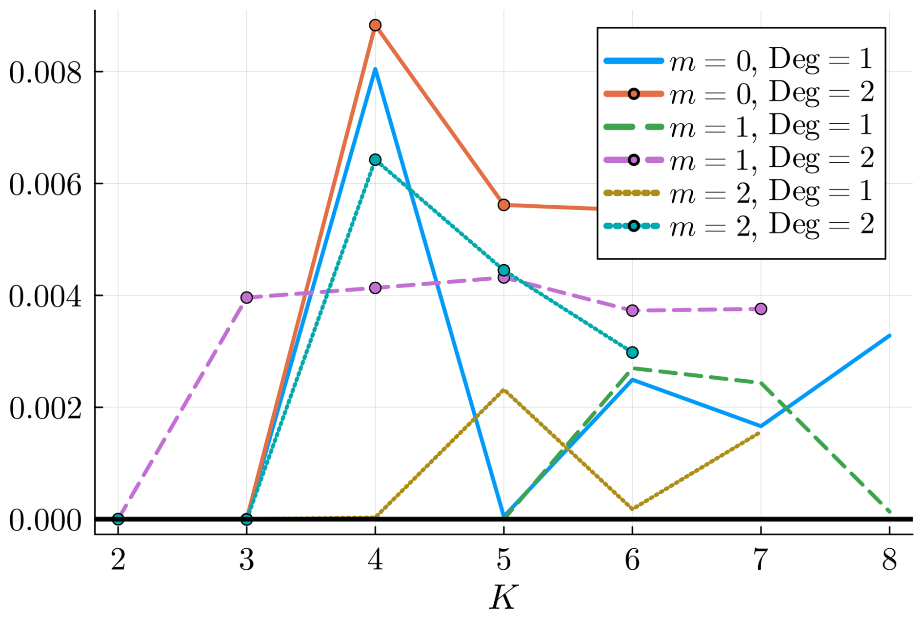
Figure F1 Relative improvement $\left({\mathcal{L}}_{\text{slice}-{\mathcal{L}}_{\text{rand}}}\right)/\left|{\mathcal{L}}_{\text{slice}}\right|$ of the final log-likelihood obtained with random or slice initialization. The slice estimate always gives a better or equal log-likelihood.

F5 Transition matrices

To finish the SHHMM inference, we estimate the transition matrices Q(t). To do so, we will first infer the filtered probability of all hidden states given the model and observations using ${\stackrel{\mathrm{̃}}{f}}_{k,t}$ and ${\stackrel{\mathrm{̃}}{\mathit{\pi }}}_{k,t}$,

$$\begin{array}{}\text{(F3)}& \begin{array}{rl}{\mathit{\gamma }}_k^{\left(n\right)}& =\mathbb{P}\left(Z^{\left(n\right)}=k\mid Y^{\left(n\right)}=y^{\left(n\right)},H^{\left(n\right)}=h^{\left(n\right)}\right)\\ & ={\displaystyle \frac{{\stackrel{\mathrm{̃}}{\mathit{\pi }}}_k{\prod }_{s=\mathrm{1}}^S{\stackrel{\mathrm{̃}}{f}}_{k,t,s}(y_s^{\left(n\right)}\mid h_s^{\left(n\right)})}{{\sum }_{l=\mathrm{1}}^K{\stackrel{\mathrm{̃}}{\mathit{\pi }}}_l{\prod }_{s=\mathrm{1}}^S{\stackrel{\mathrm{̃}}{f}}_{l,t,s}(y_s^{\left(n\right)}\mid h_s^{\left(n\right)})}}.\end{array}\end{array}$$

The maximum a posteriori estimator is then

$$\begin{array}{}\text{(F4)}& {\stackrel{\mathrm{̃}}{z}}^{\left(n\right)}={\mathrm{argmax}}_{k\in \mathit{\{}\mathrm{1},\mathrm{\cdots },K\mathit{\}}}{\mathit{\gamma }}_k^{\left(n\right)}.\end{array}$$

This yields the sequence of hidden states $\mathit{\{}{Z}^{\left(n\right)}:n\in \mathcal{D}\mathit{\}}$. The transition matrices can be estimated by counting the number of transitions on a day t from a state k to l divided by the total number of transitions from k,

$$\begin{array}{}\text{(F5)}& {\stackrel{\mathrm{̃}}{\mathbf{Q}}}_{kl}\left(t\right)={\displaystyle \frac{{\sum }_{n\in {\mathcal{N}}_t}{\mathbf{1}}_{{\stackrel{\mathrm{̃}}{z}}^{\left(n\right)}=k,{\stackrel{\mathrm{̃}}{z}}^{(n+\mathrm{1})}=l}}{{\sum }_{n\in {\mathcal{N}}_t}{\sum }_{l=\mathrm{1}}^K{\mathbf{1}}_{{\stackrel{\mathrm{̃}}{z}}^{\left(n\right)}=k,{\stackrel{\mathrm{̃}}{z}}^{(n+\mathrm{1})}=l}}}.\end{array}$$

F6 Multiple random initialization

To prevent the EM procedure from reaching an irrelevant local minimum, we run the algorithm 10 times with added noise around the initial state. For each coefficient c∈θ^(slice), we randomize as $c^{\mathrm{rand}}=c\left(\mathrm{1}+\mathit{\sigma }Z\right)$, where we take σ=0.5 and $Z\sim \mathcal{N}(\mathrm{0},\mathrm{1})$.

F7 Slice estimate initialization vs. naive random initialization

Here we show the improvement given by the slice estimate compared to pure random initialization. The log-likelihood obtained with this initialization is compared with 10 pure random initializations, where all ${\mathit{\beta }}_{\mathrm{rand}}\sim \mathcal{N}(\mathrm{0},\mathrm{0.5})$. The relative improvement is plotted in Fig. F1. It is greater than 10⁴ in 21 of 36 models shown here and equal for the other cases, including the small models with K=2 and 3 where inference is easier. Note that even an improvement of a percent can lead to quite different models, in particular regarding the interpretability of the hidden states. This can be seen in the model selection in Fig. 4, where the difference between models is typically of the order of a percent or less. Furthermore, the number of steps for Algorithm 1 to converge i_stop is smaller in most cases, e.g., for $\mathrm{3}\le K\le \mathrm{6}$ and for the best selected models, the mean of $i_{\text{stop}}^{\left(\mathrm{rand}\right)}-i_{\text{stop}}^{\left(\mathrm{slice}\right)}\simeq \mathrm{226}$.